Optimizing-Time Series Imputation with Data Quality

Abstract

Missing values in time series are not uncommon due to system failures or external interference during data collection. A multitude of imputation algorithms have been proposed to infer these missing values. However, existing methods often overlook the difference in sample data quality within the dataset. Specifically, training imputation algorithms on low-quality samples can lead to the generation of poor-quality data, which adversely affects the performance of downstream models. To address this issue, we propose integrating a data quality evaluation with the imputation process. The workflow involves imputing missing values using an imputation algorithm, evaluating the data quality of each sample, and then removing low-quality samples. Our experimental results demonstrate the effectiveness of this approach on improving the performance of downstream model across four datasets, seven input algorithms, four quality assessment methods, and two types of machine learning tasks. Additionally, we convert time series data into complex networks and find that network features can effectively explain the data quality of individual samples.

1. Introduction

Time-series data are sequential records ordered chronologically to capture changes within a system. Common examples include traffic flow measurements [1], electrocardiogram (ECG) recordings [2] and air-quality-monitoring data [3]. In practical applications, various factors, such as sensor malfunctions and electromagnetic interference, can lead to missing data in time series [4,5]. This phenomenon presents significant challenges for machine learning models aiming to detect patterns within these sequences, consequently impacting the accuracy of downstream forecasting and classification tasks. As a result, time-series imputation has become a hot topic in time-series data mining [6].

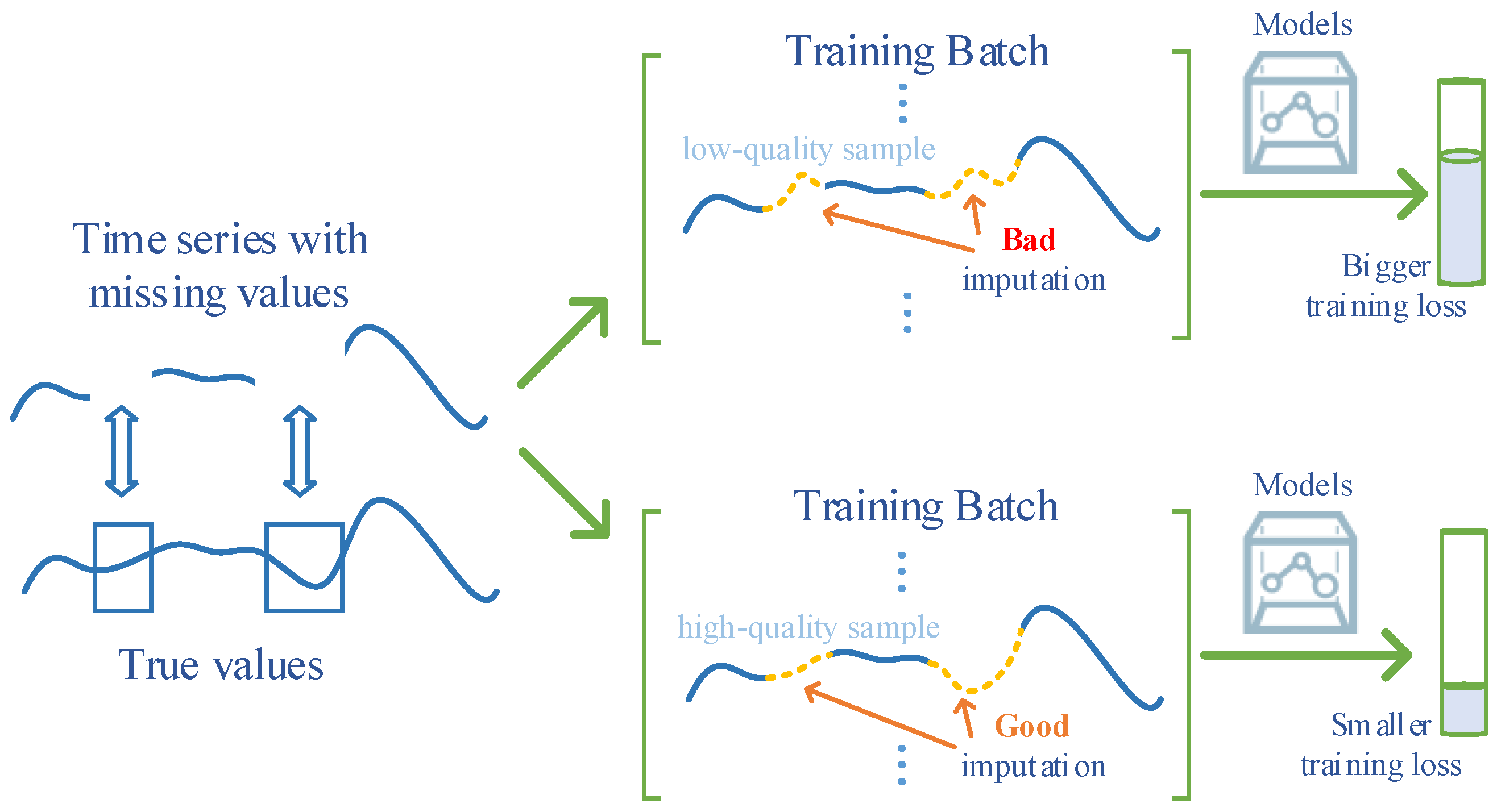
Although existing imputation methods achieve satisfactory performance by exploiting mathematical properties, similarity features, and temporal dependencies within the data, they tend to neglect the intrinsic quality of individual samples. Empirical studies have shown that variations in sample quality exist across datasets, and that low-quality samples may negatively impact model training. For example, Huang et al. [7] investigated that the performance of time-series forecasting models can also be improved by reducing the influence of low-quality samples. It should be noted that the aforementioned discussions are based on data without missing values. Consequently, it is reasonable to expect that differences in data quality may also persist among time-series samples after missing values have been imputed. This is due to the fact that existing imputation methods cannot ensure the exact recovery of true values and may inadvertently alter the original contextual associations or temporal structures within the data during the reconstruction process, as illustrated in Figure 1. Therefore, we propose integrating the concept of data quality into time-series imputation algorithms and center our investigation around the following questions: (1) Do differences in data quality persist in time-series data after imputation? This forms the foundational premise of our work. (2) If such differences exist, can existing imputation methods be optimized? This constitutes the core objective of our research. (3) Can we further identify quantifiable features that distinguish low-quality from high-quality samples within the imputed data? Addressing this key focus may provide actionable insights for future improvements in imputation algorithms.

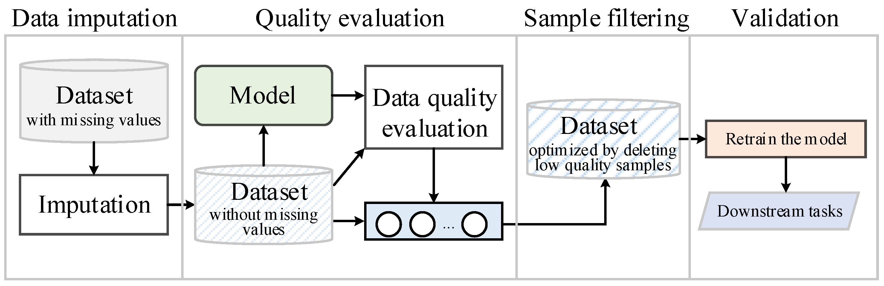
In this paper, we first demonstrate that substantial variations in quality exist among imputed samples. Importantly, this observation does not undermine the validity of existing imputation models; rather, it highlights opportunities to further enhance their performance. Building on this insight, we propose a novel quality-aware imputation framework that integrates data imputation with quality assessment. The proposed approach comprises three key steps: (1) imputation phase: apply existing imputation algorithms to generate a complete datasets without missing values; (2) evaluation phase: calculate the quality score of each sample; and (3) filtering phase: filter out low-quality samples to produce a refined, high-quality imputed datasets. Unlike the imputation algorithm, the optimization in this paper is focused on the quality of the imputed datasets, that is, retaining high-quality samples and deleting low-quality ones, rather than optimizing the missing values of the samples. Finally, we explore the relationship between complex network features and sample quality. In summary, the main contributions of this paper are as follows:

• We propose a novel method by integrating data quality evaluation algorithms and time-series imputation methods, thereby optimizing the quality of the imputed datasets.
• We comprehensively evaluate the effectiveness of our method for downstream model through extensive experiments conducted across four datasets, seven imputation algorithms, four quality assessment techniques, and two types of machine learning tasks. Specifically, the experimental results show that the prediction mean absolute error (MAE) can be reduced by up to $38.73\%$ on the Italy Air-Quality dataset; the Area Under the Precision–Recall Curve (AUPRC) score can be increased by up to $118.41\%$ on the PhysioNet 2019 dataset.
• We reveal a significant relationship between time-series data quality and complex network features, providing interpretable insights into the characteristics of low-quality samples through network-based analysis.

2. Related Work

2.1. Time-Series Imputation

2.1.1. Missing Data Mechanism

Time-series imputation refers to the process of estimating missing values in sequential data. Following Rubin’s theory [8], missing data patterns are categorized into three types: Missing Completely at Random (MCAR), where the occurrence of missing values is independent of both observed and unobserved data; Missing at Random (MAR), where missingness depends solely on observed data; and Missing Not at Random (MNAR), where missingness is influenced by both the missing and observed values. Each missing data mechanism requires distinct imputation strategies. Most existing research primarily focuses on MCAR scenarios, as fewer studies address the more complex MAR and MNAR cases. In this work, we also focus on imputation methods tailored for MCAR conditions.

2.1.2. Time-Series Imputation Methods

We begin with a concise overview of traditional approaches that employ statistical methods and machine learning algorithms, followed by an in-depth discussion of deep-learning-based techniques for time-series imputation.

Traditional Methods

These methods represent early research efforts in handling missing data. The simplest approaches involve using statistical measures such as the mean or mode for value replacement [6,9]. Regression prediction is also a commonly used method, which estimates missing values by establishing relationships between observed variables through regression equations. Another category of traditional methods relies on similarity measures, where missing values are inferred based on the similarity between data points. Common similarity metrics include Euclidean distance and cosine similarity. Representative methods in this category include: K-nearest Neighbor (KNN), which replaces missing values with the mean of the k most similar samples [10]; Hot Deck Imputation (HDI) [11], which adopts the value from the most similar sample for imputation; and Cold Deck Imputation (CDI) [12], which substitutes missing values with corresponding values from a similar sample in an external dataset. In addition, various machine learning algorithms have been adapted for imputation tasks, including Matrix Factorization [13], Expectation–Maximization [14], and Random Forest [15]. However, these methods do not adequately capture critical temporal characteristics in time-series data, such as periodicity and trend patterns, which limits their effectiveness in time-series imputation tasks.

Deep-Learning-Based Methods

Compared to traditional techniques, deep learning methods are better capable of capturing complex temporal dependencies in sequential data, thereby enabling more advanced imputation tasks such as segment-level and block-level missing patterns. In the following sections, we primarily review existing works from two distinct perspectives: generation-based and prediction-based approaches for time-series imputation.

Generation-based imputation utilizes deep generative networks to learn the underlying probability distribution from observed data and subsequently generates plausible values that align with this distribution for use as imputed results. This approach mainly relies on three categories of deep generative models: Variational Autoencoders (VAEs), Generative Adversarial Networks (GANs), and Diffusion Models. (1) VAE-based methods impute missing values by generating plausible reconstructions through the decoder, based on latent distribution parameters learned by the encoder. For example, ref. [16] directly employed a VAE for missing value imputation. The GP-VAE [17] integrates Gaussian processes into the latent space of the VAE in order to better model temporal dependencies. In [18], the authors combined the VAE with a recurrent neural network and introduced an uncertainty attenuation factor to filter out generated samples with high variance. (2) GAN-based methods, originally developed for image generation, have been increasingly adapted for time-series imputation. For instance, GRU-GAN [19] performs imputation within a GAN framework, where both the generator and discriminator utilize RNNs equipped with attenuation factors to more effectively manage missing intervals. The End-to-End Generative Adversarial Network (E²GAN) [20] builds upon GRU-GAN by integrating a denoising module, which optimizes the inputs of generator. (3) Diffusion model-based methods are another popular architecture that have demonstrated promising performance in time-series imputation. The Conditional Score-based Diffusion model for Imputation (CSDI) [21] is a representative model in this category. It uses subsets of observed data as conditional information to guide the generation of missing segments. However, despite its effectiveness, the large parameter size of CSDI hinders its scalability when applied to complex multivariate time series. To address this limitation, researchers have proposed several improved variants, such as Structured State Space Diffusion (SSSD) [22] and Conditional Schrödinger Bridge methods for probabilistic time-series imputation (CSBI) [23].

Prediction-based imputation approaches leverage time-series forecasting models to estimate missing values. In 2023, TimesNet [24] integrated the tasks of prediction, classification, and imputation within a single model and achieved state-of-the-art performance. Inspired by TimesNet, the time-series prediction model can also be used for imputation. The process utilizes historical observations and missing patterns as input features for the model, while the predicted outputs are used to construct reconstructed sequences, in which the values at previously missing positions correspond to the imputed results. We review these methods based on their underlying neural architectures: (1) RNN-based methods: GRU-D [25] is a representative model in this field. It incorporates information about missing intervals as input features and introduces a decay mechanism into recurrent neural networks, enabling the model to effectively capture both temporal patterns and characteristics of missing data. Building upon GRU-D, researchers have proposed several improved approaches, such as Bidirectional Recurrent Imputation for Time Series (BRITS) [26] and Multi-directional Recurrent Neural Networks (M-RNNs) [27]. (2) CNN-based methods primarily employ convolutional neural network architectures specifically designed for time-series forecasting tasks. For example, Temporal Convolutional Networks (TCNs) [28], which is a class of classical convolutional networks, are widely used in time-series data mining. In addition, Multi-scale Isometric Convolution Network (MICN) [29] and TimesNet are also representative prediction models based on convolution, capable of performing the time-series imputation task. (3) GNN-based methods have demonstrated remarkable capability in capturing variable dependencies within multivariate time series. For time-series imputation, representative approaches include Spectral Temporal Graph Neural Network (StemGNN) [30] and Graph Recurrent Imputation Network (GRIN) [31], which integrate graph learning with the imputation process, as well as the Spatiotemporal Point Inference Network (SPIN) [32], which incorporates spectral graph convolution techniques to enhance modeling accuracy. (4) Transformer-based method: Following Informer’s breakthrough in time-series prediction [33], transformer architectures have become dominant in recent imputation research. Representative works include the Deep learning method for Missing Value Imputation (DeepMVI) [34], and Self-attention-based Imputation for Time Series (SAITS) [35]. DeepMVI integrates convolutional and transformer modules to achieve effective missing value imputation, while SAITS enhances the attention mechanism through diagonal masking to more accurately address missing patterns.

In summary, the exceptional nonlinear fitting capability of neural networks has given rise to a variety of deep-learning-based methods for time-series imputation, which have exhibited superior performance across multiple domains. However, this paper shows that their effectiveness can be further improved by incorporating a data quality evaluation module. In real-world scenarios, the collection of time-series data is frequently affected by electromagnetic interference, equipment malfunctions, and other factors that introduce noise. When such noisy observational data are used to train imputation models, the resulting estimates of missing values may be inaccurate, which can hinder the model’s ability to learn true temporal dependencies. To address this challenge, we propose augmenting imputation methods with a data quality evaluation module to filter low-quality samples in training data. The following section reviews relevant work in data quality evaluation.

2.2. Data Quality Evaluation

Data quality originally emerged in the fields of data management and data cleaning. In 2021, Andrew Ng [36] introduced the concept of “data-centric AI”, which highlights the critical role of data in AI systems. Zhou et al. [37] defined sample quality as the extent to which data meets specific requirements. So far, existing works have primarily addressed the “what if” question examining how the model behaves when it is not trained on or numerically influenced by a particular sample.

From the perspective of how data impact model performance, this paper reviews the following representative studies on data quality evaluation: (1) Influence function-based approach: In 2017, Koh et al. [38] proposed the influence function method, which estimates the change in model performance on the validation set when a particular training sample is upweighted or removed, using gradient information. This change was used as an indicator of the quality of this sample. Subsequently, Hara et al. [39] introduced an improved SGD-influence method that extends the influence function to non-convex objectives, such as deep neural networks, thereby broadening its applicability. (2) Shapley value-based method: The Shapley value was proposed by L. S. Shapley in 1953. It defines a member’s profit in cooperation as the average of the marginal contributions that he generates for all coalitions he participates in. Jia et al. [40] used it for data quality assessment, in which the k-nearest neighbor classifier was used as a surrogate model to calculate sample Shapley values. (3) Loss gradient-based methods, which directly quantify sample data quality based on the loss gradient of each sample, exhibit lower computational complexity compared to influence function and Shapley value-based approaches. Pual et al. [41] proposed a direct method named gradient normalization (Grand) to identify important samples by using the norm of the loss gradient computed for individual samples. Agarwal et al. [42] demonstrated that simpler samples tend to exhibit lower variance. Accordingly, they introduced a metric called gradient variance (VoG) to evaluate data quality.

3. Methodology

3.1. Data Insight

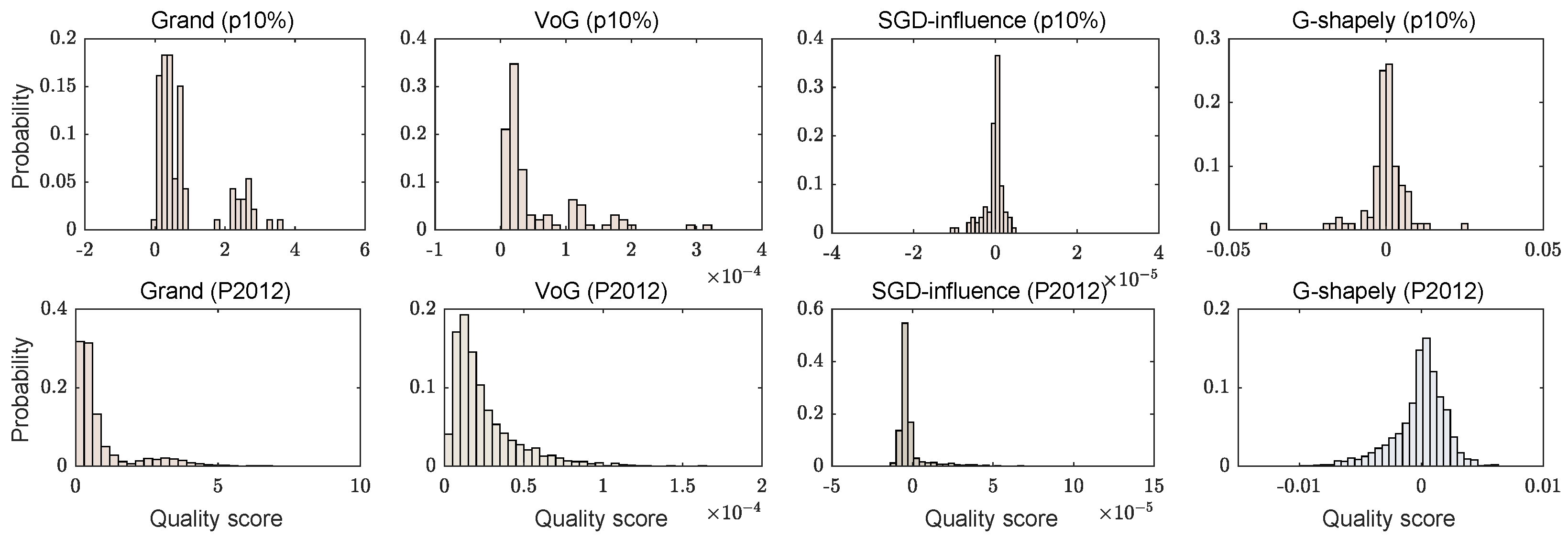
Figure 2 illustrates the distribution of sample quality scores generated by various evaluation algorithms. Specifically, the first row of images in Figure 1 presents the statistical results of the quality scores of the datasets imputed by SAITS for the Italy Air-Quality datasets. The second row presents the statistical information on the PhysioNet 2012 datasets. For more information on the datasets, please refer to Section 4.1. From the experimental results, most distributions exhibit a distinct long-tail pattern, with the exception of the G-Shapley assessment results for the prediction task, which closely resemble a bell-shaped (Gaussian-like) distribution. These observations confirm the presence of quality differences among samples following the imputation process. This evidence strongly supports the central premise of this study: that data quality evaluation can be effectively utilized to enhance time-series imputation algorithms. Code is available at gitee (https://gitee.com/jimapp330/Imputation-withDataQuality.git (accessed on 1 July 2026)).

3.2. Our Method

This paper proposes a novel approach to improving data imputation performance by optimizing data quality. Unlike traditional methods that focus on enhancing model architecture, we introduce an innovative framework that integrates imputation algorithms with a data quality evaluation module. Specifically, we present an “impute-evaluate-filter” strategy (as illustrated in Figure 3), which first performs data imputation and then filters the imputed samples based on quality metrics, thereby producing a high-quality imputed datasets. The proposed methodology consists of three core steps, which are described below.

3.2.1. Imputation

First, we need to train an imputation model. In this paper, the imputation model can be selected from the-state-of-the-art deep-learning-based imputation models. In existing works, the training strategy is to first construct the time series without missing values into a dataset of missing values according to a certain missing ratio and missing pattern. Then, model learning is guided through reconstruction. The training process can be expressed as follows:

$${\mathcal{M}}_{train}=Train({\mathcal{M}}_0,{\mathcal{D}}_{train}),$$

(1)

where ${\mathcal{M}}_0$ is an imputation model with randomly initialized parameters, including but not limited to GPVAE, SSGAN, CSDI, GRU-D, TimesNet, StemGNN, and SAITS. ${\mathcal{M}}_{train}$ corresponds to the trained model. ${\mathcal{D}}_{train}$ is the train set.

Then, we use the trained model ${\mathcal{M}}_{train}$ to perform imputation on missing values within the original datasets ${\mathcal{D}}_{original}$:

$${\mathcal{D}}_{imputation}=Imputation({\mathcal{M}}_{train},{\mathcal{D}}_{original}),$$

(2)

where ${\mathcal{D}}_{imputation}$ is the original datasets after imputation. Equations (1) and (2) capture the core computational flow of conventional imputation methods, which generate completed datasets for downstream applications. As mentioned before, we think current imputation may damage the contextual relationships or temporal structures within the original data during the recovery process. Therefore, we introduce additional sample evaluation and filtering steps to deal with this issues.

3.2.2. Evaluation

Data quality assessment algorithms aim to quantify the extent to which individual samples contribute positively or negatively to model learning. Within the framework of this paper, our objective is to first use the data quality evaluation algorithm to evaluate the imputed datasets ${\mathcal{D}}_{imputation}$, enabling subsequent filtering of low-quality instances. The process is given as follows:

$$\mathcal{Q}=Evaluation({\mathcal{D}}_{imputation},{\mathcal{A}}_{quality}).$$

(3)

The quality evaluation algorithm ${\mathcal{A}}_{quality}$ could select but not is limited to Grand, VoG, SGD-influence and G-Shapley. The fundamental operating principles of these selected algorithms are briefly outlined below:

(1)

Grand is defined as the expected value of the norm of the sample gradient [41]. Formally:

$$Gran{d}_t(x,y)={\mathbb{E}}_{{\mathbf{w}}_t}{\parallel g_t(x,y)\parallel }_2,$$

(4)

where the sample gradient at t-th training step, $g_t(x,y)={\nabla }_{{\mathbf{w}}_t}\mathcal{L}(p({\mathbf{w}}_t,x),y)$ and $t=1,\dots ,T$. ${\mathbf{w}}_t$ is a vector representing the parameters of model at t-th training step. Loss function $\mathcal{L}(·)$ is defined as the prediction loss or classification loss. $p({\mathbf{w}}_t,x)$ is the output of model. y is the true value or label.

(2)

VoG is defined as the variance in Gradient [42]. More specifically, a sample’s quality is evaluated based on its variance in the gradient values. The samples that are challenging for the model to learn tend to exhibit larger gradient variance throughout training. $S_t$ can be defined as the gradient of the model parameters at t-th training step, and $\mu$ the average gradient over k training epochs; VoG can be calculated as follows:

$$Vo{G}_t=\sqrt{{\displaystyle \frac{1}{k}}\sum _{t=1}^k{\left(S_t-\mu \right)}^2}.$$

(5)

In Equation (5), $Vo{G}_t$ is a vector; we convert it to a scalar and get the VoG score.

$$VoG(x,y)={\displaystyle \frac{1}{\left|Vo{G}_t\right|}}\sum _{v\in Vo{G}_t}v.$$

(6)

(3)

SGD-influence: Given a sample $z_j$ at step t, SGD-influence refers to the parameter difference ${\theta }_{-j}^{\left[t\right]}-{\theta }^{\left[t\right]}$ [39]. If the sample $z_j$ is used at step $\pi \left(j\right)$, after T steps, SGD-influence can be estimated as follows:

$${\theta }_{-j}^{\left[T\right]}-{\theta }^{\left[T\right]}\approx {\displaystyle \frac{{\eta }_{\pi \left(j\right)}}{|S_{\pi \left(j\right)}|}}{Z}_{T-1}{Z}_{T-2}\cdots Z_{\pi \left(j\right)+1}g(z_j;{\theta }^{\left[\pi \right(j\left)\right]}),$$

(7)

where $Z_t=\mathit{I}-{\eta }_t{H}^{\left[t\right]}$. $H^{\left[t\right]}$ is the Hessian matrix. $\mathit{I}$ is the identity matrix. $S_{\pi \left(j\right)}$ denotes the set of sample indices used in the $\pi \left(j\right)$-th step, and ${\eta }_{\pi \left(j\right)}>0$ is the learning rate. The gradient of the loss function $g(z_i;{\theta }^{\left[t\right]})={\nabla }_{\theta }\mathcal{L}(z_i;{\theta }^{\left[t\right]})$. Direct calculation of the Hessian matrix $H^{\left[t\right]}$ is computationally expensive. Therefore, its approximate value can be obtained by calculating $H^{\left[t\right]}{u}^{\left[t\right]}$:

$$H^{\left[t\right]}{u}^{\left[t\right]}={\displaystyle \frac{1}{|S_t|}}\sum _{i\in S_t}{\nabla }_{\theta }〈u^{\left[t\right]},g(z_i;{\theta }^{\left[t\right]})〉,$$

(8)

where $u^{\left[t\right]}$ is the derivative of the model f for an x sample in the validated set.

(4)

G-Shapley. Data Shapley is proposed according to the Shapley value defined in game theory. G-Shapley is an approximation of Data Shapley based on the stochastic gradient descent algorithm [43]. Given the training datset D, Data Shapley refers to the sum of performance changing over all subsets of D not containing sample i. Its expression is given as follows:

$${\varphi }_i=C\sum _{S\subseteq D-\left\{i\right\}}{\displaystyle \frac{V(S\cup \{i\left\}\right)-V\left(S\right)}{\left(\genfrac{}{}{0pt}{}{n-1}{S}\right)}},$$

(9)

where C is an arbitrary constant. V(S) is the performance score of a model trained on data S. In common, we use the test dataset to obtain V(S). As shown in Equation (9), computing Data Shapley requires computing all the possible marginal contributions which is exponentially large in the train data size. In addition, for each $S\subseteq D$, computing V(S) involves learning a model on S. As a consequence, calculating the exact Shapley value is not tractable for real scenario. Gradient Shapley (G-Shapley) is a simple approximation for Data Shapley by training the model with only one pass through the training data. Assume the length of the training dataset is n, ${\pi }^t$ is a random permutation of training data at t-th test time, and ${\theta }_0^t$ denotes the random initialization parameters. For each sample $j\in \{1,\cdots ,n\}$ in the training dataset, we implement the process as follows:

$$\begin{array}{cc}\hfill & {\theta }_j^t={\theta }_{j-1}^t-\alpha {\nabla }_{\theta }\mathcal{L}({\pi }^t\left[j\right];{\theta }_{j-1})\hfill \\ \hfill & v_j^t=V\left({\theta }_j^t\right)\hfill \\ \hfill & {\varphi }_{{\pi }^t\left[j\right]}={\displaystyle \frac{t-1}{t}}{\varphi }_{{\pi }^{t-1}\left[j\right]}+{\displaystyle \frac{1}{t}}(v_j^t-v_j^{t-1}),\hfill \end{array}$$

(10)

where $\alpha$ represents the learning rate, $v_j^t$ is the performance score of sample j at t-th test time, and $v_j^t-v_{j-1}^t$ is the marginal contribution is the change in model’s performance.

3.2.3. Filtering

According to the quality score, we filter out poor-quality samples:

$${\mathcal{D}}_{filter}=Filter({\mathcal{D}}_{imputation},\mathcal{Q}).$$

(11)

Specifically, we sort the samples in ascending order based on their quality score and delete the top-k lowest-quality samples, thereby obtaining the optimized imputed datasets ${\mathcal{D}}_{filter}$.

Upon obtaining the filtered ${\mathcal{D}}_{filter}$, we use it to retrain a new model. Our experiments demonstrate that the optimized datasets significantly improve model performance in both prediction and classification tasks (see Section 4). Notably, our filtering strategy is exclusively applied to the training set, while the validation and test sets remain unmodified to ensure unbiased evaluation. The complete procedure is formalized in Algorithm 1.

Algorithm 1 Optimizing Time-Series Imputation with Data Quality

Require:  Train set ${\mathcal{D}}_{train}$, the imputation algorithm $\mathcal{M}$  Ensure:  The optimized imputed datasets ${\mathcal{D}}_{filter}$    1: Train the imputation algorithm based on train set (see Equation (1))    2: Obtain imputed datasets ${\mathcal{D}}_{imputation}$ using imputation algorithm (see Equation (2))    3: Calculate sample quality score $\mathcal{Q}$ (see Equation (3))    4: Sort the samples in ascending order according to their quality score    5: Delete the top-k samples to obtain the optimized imputed datasets ${\mathcal{D}}_{filter}$ (see Equation (11))    6: Return ${\mathcal{D}}_{filter}$

4. Experiments

4.1. Experimental Setup

Target: This section presents the experimental validation of the proposed framework, focusing on two key research questions: (1) Effectiveness validation: How effective is the proposed quality-aware imputation optimization method in enhancing performance on downstream tasks? (2) Relationship exploration: Are there characteristics that distinguish low-quality from high-quality samples in the imputed data?

Approach: For the first question, we compare the performance of downstream models trained on two types of imputed data: (1) the original training data repaired using imputation algorithms, and (2) the imputed data further refined through our quality-aware optimization procedure. Model performance is assessed on unmodified validation and test sets. In experiments, we employ seven distinct baseline imputation algorithms: three generation-based methods (GPVAE [17], SSGAN [44], CSDI [21]) and four prediction-based algorithms (GRUD [25], TimesNet [24], StemGNN [30] and SAITS [35]). For the data quality evaluation phase, we select four representative algorithms: Grand, VoG, SGD-influence, and G-Shapley. For the second question, the relationship between the sample quality and time-series features derived from complex networks is assessed.

Datasets: We conducted experiments on four datasets: Italy Air-Quality (https://archive.ics.uci.edu/dataset/360/air+quality (accessed on 1 July 2026)), ETT (https://github.com/zhouhaoyi/ETDataset (accessed on 1 July 2026)), PhysioNet 2012 (https://www.physionet.org/content/challenge-2012/1.0.0/ (accessed on 1 July 2026)), and PhysioNet 2019 (https://physionet.org/content/challenge-2019/1.0.0/ (accessed on 1 July 2026)). An overview of the datasets’ information is presented in

Table 1. Data information used in this work.

Dataset	ETT	Italy Air-Quality	PhysioNet2012	PhysioNet2019
# of Total Samples	358	774	3997	4927
Features	7	13	35	33
Sample Sequence Length	48	12	48	48
Time Interval	1 h	1 h	1 h	1 h
Original Missing Rate (%)	0	0	79.3	73.9

. The Italy Air-Quality and ETT datasets are used for the prediction task. Since there are no missing values in these two datasets, in the experiment, we adopted three missing patterns (subsequence missing (abbreviated as s), point missing (abbreviated as p), and block missing (abbreviated as b)) along with different missing proportions to process the data. The PhysioNet 2012 and PhysioNet 2019 datasets are used for the classification task. Due to their naturally high missing data rates (approximately $80\%$), we do not introduce any additional missing values. For the prediction task, we utilize two widely adopted evaluation metrics: the Mean Absolute Error (MAE) and Mean Squared Error (MSE). For the classification task, we use accuracy, the F1 score and the Area Under the Precision–Recall Curve (AUPRC) [45] to evaluate model performance. As described in Algorithm 1, the data quality evaluation algorithm only involves ${\mathcal{D}}_{train}$, outputs ${\mathcal{D}}_{filter}$, and the downstream model training is conducted on the ${\mathcal{D}}_{filter}$, while downstream model testing uses the test datasets.

4.2. Performance on Prediction Task

A standard LSTM architecture is employed for the prediction task.

Table 2. Italy Air-Quality datasets (part 1: GPVAE, SSGAN, and CSDI).

Scenario		GPVAE		SSGAN		CSDI
Type	Algorithm	MSE	MAE	MSE	MAE	MSE	MAE
s (10%)	LSTM	0.6069 ± 0.0262	1.7760 ± 0.0446	0.5466 ± 0.0036	1.8120 ± 0.0131	0.5289 ± 0.0087	0.5379 ± 0.0268
	Grand	0.5981 ± 0.0085	1.7737 ± 0.0041	0.5681 ± 0.0044	1.7785 ± 0.0212	0.5339 ± 0.0380	0.6664 ± 0.0894
	VoG	0.5842 ± 0.0083	1.7200 ± 0.0037	0.5370 ± 0.0173	1.7656 ± 0.0203	0.5099 ± 0.0275	0.6081 ± 0.0658
	SGD-influence	0.6161 ± 0.0866	1.5727 ± 0.4386	0.5520 ± 0.0796	1.4083 ± 0.1391	0.4962 ± 0.0276	0.5606 ± 0.0446
	G-Shapley	0.5806 ± 0.0160	1.7057 ± 0.0309	0.5415 ± 0.0146	1.7715 ± 0.0352	0.4850 ± 0.0337	0.5129 ± 0.0265
p (10%)	LSTM	0.4685 ± 0.0039	1.4330 ± 0.0038	0.4906 ± 0.0064	1.4647 ± 0.0034	0.2023 ± 0.0051	0.4128 ± 0.0112
	Grand	0.4441 ± 0.0051	1.4168 ± 0.0127	0.5697 ± 0.0109	1.7937 ± 0.0286	0.1747 ± 0.0047	0.4447 ± 0.0011
	VoG	0.4218 ± 0.0359	1.4441 ± 0.0226	0.5370 ± 0.0173	1.7656 ± 0.0203	0.1466 ± 0.0114	0.3603 ± 0.0074
	SGD-influence	0.4442 ± 0.0111	1.1112 ± 0.0216	0.5668 ± 0.0646	1.4321 ± 0.0512	0.1734 ± 0.0070	0.3880 ± 0.0415
	G-Shapley	0.4480 ± 0.0478	1.3212 ± 0.2626	0.5346 ± 0.0075	1.7770 ± 0.0141	0.1526 ± 0.0111	0.3552 ± 0.0048
p (50%)	LSTM	0.3836 ± 0.0146	0.5231 ± 0.1778	0.4923 ± 0.0068	0.7624 ± 0.0751	0.7001 ± 0.0232	1.2032 ± 0.0639
	Grand	0.3614 ± 0.0041	0.4882 ± 0.0022	0.4634 ± 0.0055	0.8356 ± 0.0027	0.6746 ± 0.0102	1.1488 ± 0.0589
	VoG	0.3618 ± 0.0035	0.4949 ± 0.0017	0.4662 ± 0.0075	0.8450 ± 0.0149	0.6990 ± 0.0012	1.1684 ± 0.0269
	SGD-influence	0.3505 ± 0.0331	0.4088 ± 0.1161	0.4399 ± 0.0299	0.6382 ± 0.2055	0.6968 ± 0.0157	1.1714 ± 0.0248
	G-Shapley	0.3674 ± 0.0066	0.5076 ± 0.0133	0.4236 ± 0.0122	0.5484 ± 0.0640	0.7185 ± 0.0341	1.1914 ± 0.0858
b (10%)	LSTM	0.4848 ± 0.0032	1.2204 ± 0.0104	0.4834 ± 0.0052	1.5211 ± 0.0123	0.4254 ± 0.0181	1.5433 ± 0.0896
	Grand	0.5079 ± 0.0219	1.1346 ± 0.0501	0.4843 ± 0.0066	1.5208 ± 0.0190	0.4666 ± 0.0053	1.6654 ± 0.0302
	VoG	0.4893 ± 0.0077	1.2178 ± 0.0211	0.4820 ± 0.0020	1.5191 ± 0.0136	0.4334 ± 0.0167	1.5761 ± 0.0753
	SGD-influence	0.4954 ± 0.0072	1.2017 ± 0.0061	0.4687 ± 0.0651	1.3208 ± 0.3541	0.4160 ± 0.0140	1.4412 ± 0.0817
	G-Shapley	0.4864 ± 0.0067	1.2113 ± 0.0132	0.4859 ± 0.0045	1.5072 ± 0.0062	0.4117 ± 0.0372	1.5986 ± 0.1171

,

Table 3. Italy Air-Quality datasets (part 2: comparison of GRUD, TimesNet, StemGNN, and SAITS).

Scenario		GRUD		TimesNet		StemGNN		SAITS
Type	Algorithm	MSE	MAE	MSE	MAE	MSE	MAE	MSE	MAE
s (10%)	LSTM	0.7092 ± 0.0036	2.0865 ± 0.0161	0.7064 ± 0.0065	1.8812 ± 0.0292	0.6659 ± 0.0029	2.4489 ± 0.0425	0.5362 ± 0.0043	1.8708 ± 0.0199
	Grand	0.7162 ± 0.0503	2.1787 ± 0.2991	0.5684 ± 0.0329	1.4741 ± 0.0349	0.6806 ± 0.0347	2.2659 ± 0.0996	0.6667 ± 0.0087	1.8317 ± 0.0312
	VoG	0.7166 ± 0.0183	2.0568 ± 0.0083	0.7133 ± 0.0242	1.5320 ± 0.3086	0.6604 ± 0.0051	2.4551 ± 0.0162	0.5674 ± 0.0399	1.9854 ± 0.1905
	SGD-influence	0.7651 ± 0.0196	2.0978 ± 0.0723	0.6779 ± 0.0075	1.4849 ± 0.0761	0.6442 ± 0.0234	1.9921 ± 0.3765	0.4526 ± 0.0171	1.2107 ± 0.0201
	G-Shapley	0.7205 ± 0.0084	2.0929 ± 0.0160	0.6947 ± 0.0360	1.6994 ± 0.2787	0.6522 ± 0.0047	2.3964 ± 0.0265	0.5402 ± 0.0075	1.8558 ± 0.0199
p (10%)	LSTM	0.4497 ± 0.0045	1.4008 ± 0.0021	0.4686 ± 0.0070	1.4310 ± 0.0053	0.4689 ± 0.0037	1.4796 ± 0.0092	0.4439 ± 0.0341	1.4392 ± 0.0173
	Grand	0.4064 ± 0.0026	1.4164 ± 0.0119	0.4596 ± 0.0048	1.3905 ± 0.0009	0.5931 ± 0.1970	1.7824 ± 0.4479	0.4098 ± 0.0533	1.4298 ± 0.0196
	VoG	0.4356 ± 0.0356	1.3015 ± 0.1725	0.4314 ± 0.0063	1.4361 ± 0.0243	0.4637 ± 0.0130	1.4886 ± 0.0064	0.4129 ± 0.0130	1.4141 ± 0.0435
	SGD-influence	0.4268 ± 0.0494	1.1224 ± 0.2577	0.4257 ± 0.0164	0.9025 ± 0.0573	0.4394 ± 0.0155	1.3646 ± 0.1931	0.4425 ± 0.0711	1.2340 ± 0.3155
	G-Shapley	0.4264 ± 0.0081	1.4144 ± 0.0122	0.4439 ± 0.0020	1.4293 ± 0.0114	0.4549 ± 0.0047	1.4933 ± 0.0077	0.4153 ± 0.0128	1.4058 ± 0.1008
p (50%)	LSTM	0.5649 ± 0.0033	1.2445 ± 0.0093	0.5287 ± 0.0024	0.9650 ± 0.0146	0.4945 ± 0.0087	1.1204 ± 0.0382	0.4825 ± 0.0079	0.9279 ± 0.0106
	Grand	0.5297 ± 0.0023	1.2010 ± 0.0037	0.4931 ± 0.0036	0.9191 ± 0.0026	0.4421 ± 0.0016	1.0928 ± 0.0058	0.4773 ± 0.0205	0.9155 ± 0.0034
	VoG	0.5233 ± 0.0163	1.1415 ± 0.0797	0.4884 ± 0.0238	0.8375 ± 0.1224	0.4448 ± 0.0041	1.0924 ± 0.0018	0.4954 ± 0.0291	0.9204 ± 0.0102
	SGD-influence	0.4943 ± 0.0417	0.7424 ± 0.2277	0.4195 ± 0.0064	0.5913 ± 0.0169	0.4595 ± 0.0374	0.8583 ± 0.1690	0.4822 ± 0.0092	0.8576 ± 0.0158
	G-Shapley	0.5073 ± 0.0398	0.9415 ± 0.2694	0.4622 ± 0.0207	0.7828 ± 0.1175	0.4630 ± 0.0026	1.1397 ± 0.0036	0.4372 ± 0.0078	0.9126 ± 0.0094
b (10%)	LSTM	0.5206 ± 0.0030	1.4827 ± 0.0128	0.5357 ± 0.0020	1.3399 ± 0.0066	0.4381 ± 0.0032	1.3491 ± 0.0106	0.4943 ± 0.0175	1.9141 ± 0.0206
	Grand	0.4999 ± 0.0052	1.2988 ± 0.0714	0.5476 ± 0.0572	1.2716 ± 0.0520	0.4465 ± 0.0026	1.2628 ± 0.0589	0.4528 ± 0.0027	1.7850 ± 0.0129
	VoG	0.4914 ± 0.0080	1.3575 ± 0.0401	0.5291 ± 0.0043	1.3205 ± 0.0172	0.4371 ± 0.0016	1.2731 ± 0.0252	0.4527 ± 0.0013	1.7579 ± 0.0215
	SGD-influence	0.5199 ± 0.0061	1.4300 ± 0.0034	0.5416 ± 0.0042	1.3022 ± 0.0127	0.4453 ± 0.0049	1.3535 ± 0.0086	0.4687 ± 0.0113	1.8571 ± 0.0122
	G-Shapley	0.5340 ± 0.0008	1.4686 ± 0.0157	0.5310 ± 0.0052	1.3573 ± 0.0231	0.4424 ± 0.0062	1.3584 ± 0.0078	0.4727 ± 0.0098	1.8980 ± 0.0083

,

Table 4. ETT datasets (part 1: GPVAE, SSGAN, and CSDI).

Type	Algorithm	GPVAE		SSGAN		CSDI
		MSE	MAE	MSE	MAE	MSE	MAE
s (10%)	LSTM	$0.9052\pm 0.0319$	$1.1292\pm 0.0601$	$0.8886\pm 0.0268$	$1.1957\pm 0.0701$	$0.9772\pm 0.0259$	$1.4738\pm 0.1067$
	Grand	$\mathbf{0.8519}\pm \mathbf{0.0266}$	$\mathbf{1.0469}\pm \mathbf{0.0593}$	$\mathbf{0.8743}\pm \mathbf{0.0693}$	$\mathbf{1.1503}\pm \mathbf{0.1576}$	$1.0069\pm 0.0107$	$1.5818\pm 0.0460$
	VoG	$\mathbf{0.8059}\pm \mathbf{0.0250}$	$\mathbf{0.9748}\pm \mathbf{0.0500}$	$\mathbf{0.8461}\pm \mathbf{0.0321}$	$\mathbf{1.0757}\pm \mathbf{0.0925}$	$\mathbf{0.9354}\pm \mathbf{0.0136}$	$\mathbf{1.3333}\pm \mathbf{0.0576}$
	SGD-influence	$\mathbf{0.7855}\pm \mathbf{0.0115}$	$\mathbf{0.9414}\pm \mathbf{0.0270}$	$\mathbf{0.7927}\pm \mathbf{0.0315}$	$\mathbf{1.0324}\pm \mathbf{0.0243}$	$\mathbf{0.9161}\pm \mathbf{0.0091}$	$\mathbf{1.2753}\pm \mathbf{0.0157}$
	G-Shapley	$\mathbf{0.8180}\pm \mathbf{0.0173}$	$\mathbf{0.9995}\pm \mathbf{0.0337}$	$\mathbf{0.8125}\pm \mathbf{0.0533}$	$\mathbf{1.0318}\pm \mathbf{0.1187}$	$\mathbf{0.9223}\pm \mathbf{0.0353}$	$\mathbf{1.3194}\pm \mathbf{0.0767}$
p (10%)	LSTM	$0.9712\pm 0.0033$	$1.3399\pm 0.0049$	$0.9594\pm 0.0094$	$1.2938\pm 0.0184$	$0.9957\pm 0.0405$	$1.4507\pm 0.1616$
	Grand	$\mathbf{0.9447}\pm \mathbf{0.0364}$	$\mathbf{1.2763}\pm \mathbf{0.0823}$	$\mathbf{0.9518}\pm \mathbf{0.0242}$	$1.2955\pm 0.0877$	$1.0238\pm 0.0235$	$1.5387\pm 0.0755$
	VoG	$\mathbf{0.9175}\pm \mathbf{0.0334}$	$\mathbf{1.2321}\pm \mathbf{0.0659}$	$\mathbf{0.8824}\pm \mathbf{0.0136}$	$\mathbf{1.1262}\pm \mathbf{0.0206}$	$\mathbf{0.9300}\pm \mathbf{0.0331}$	$\mathbf{1.2498}\pm \mathbf{0.0918}$
	SGD-influence	$\mathbf{0.9007}\pm \mathbf{0.0299}$	$\mathbf{1.2294}\pm \mathbf{0.0541}$	$\mathbf{0.8953}\pm \mathbf{0.0404}$	$\mathbf{1.1753}\pm \mathbf{0.0914}$	$\mathbf{0.8923}\pm \mathbf{0.0196}$	$\mathbf{1.2062}\pm \mathbf{0.0392}$
	G-Shapley	$\mathbf{0.8833}\pm \mathbf{0.0022}$	$\mathbf{1.1877}\pm \mathbf{0.0198}$	$\mathbf{0.8866}\pm \mathbf{0.0077}$	$\mathbf{1.1404}\pm \mathbf{0.0203}$	$\mathbf{0.8957}\pm \mathbf{0.0136}$	$\mathbf{1.1382}\pm \mathbf{0.0242}$
p (50%)	LSTM	$1.0353\pm 0.0170$	$1.6280\pm 0.0373$	$1.0418\pm 0.0321$	$1.5878\pm 0.1017$	$1.0326\pm 0.0129$	$1.6232\pm 0.0489$
	Grand	$1.1884\pm 0.0579$	$2.2628\pm 0.2644$	$1.0784\pm 0.0133$	$1.7261\pm 0.0460$	$\mathbf{0.9912}\pm \mathbf{0.0281}$	$\mathbf{1.5515}\pm \mathbf{0.0754}$
	VoG	$1.0557\pm 0.0582$	$1.6776\pm 0.1497$	$\mathbf{1.0261}\pm \mathbf{0.0536}$	$\mathbf{1.5190}\pm \mathbf{0.1616}$	$\mathbf{0.9652}\pm \mathbf{0.0222}$	$\mathbf{1.4645}\pm \mathbf{0.1121}$
	SGD-influence	$\mathbf{0.9832}\pm \mathbf{0.0230}$	$\mathbf{1.5159}\pm \mathbf{0.0739}$	$\mathbf{0.9841}\pm \mathbf{0.0241}$	$\mathbf{1.4433}\pm \mathbf{0.0393}$	$\mathbf{0.9676}\pm \mathbf{0.0248}$	$\mathbf{1.4478}\pm \mathbf{0.0712}$
	G-Shapley	$\mathbf{0.9808}\pm \mathbf{0.0055}$	$\mathbf{1.4910}\pm \mathbf{0.0171}$	$\mathbf{0.9715}\pm \mathbf{0.0174}$	$\mathbf{1.3890}\pm \mathbf{0.0439}$	$\mathbf{0.9462}\pm \mathbf{0.0396}$	$\mathbf{1.3633}\pm \mathbf{0.0884}$
b (10%)	LSTM	$1.0074\pm 0.0595$	$1.4952\pm 0.1561$	$0.8580\pm 0.0054$	$1.1546\pm 0.0234$	$0.9713\pm 0.0211$	$1.4098\pm 0.0567$
	Grand	$1.0111\pm 0.0341$	$1.5257\pm 0.0707$	$0.8582\pm 0.0103$	$1.2008\pm 0.0850$	$\mathbf{0.9466}\pm \mathbf{0.0073}$	$\mathbf{1.3350}\pm \mathbf{0.0345}$
	VoG	$\mathbf{0.8841}\pm \mathbf{0.0224}$	$\mathbf{1.1923}\pm \mathbf{0.0311}$	$0.8638\pm 0.0079$	$1.1609\pm 0.0196$	$\mathbf{0.9223}\pm \mathbf{0.0039}$	$\mathbf{1.2574}\pm \mathbf{0.0197}$
	SGD-influence	$\mathbf{0.9117}\pm \mathbf{0.0173}$	$\mathbf{1.2431}\pm \mathbf{0.0428}$	$\mathbf{0.8425}\pm \mathbf{0.0234}$	$\mathbf{1.1365}\pm \mathbf{0.0457}$	$\mathbf{0.9433}\pm \mathbf{0.0375}$	$\mathbf{1.3089}\pm \mathbf{0.0913}$
	G-Shapley	$\mathbf{0.8750}\pm \mathbf{0.0480}$	$\mathbf{1.1964}\pm \mathbf{0.0992}$	$0.8673\pm 0.0044$	$\mathbf{1.1061}\pm \mathbf{0.0273}$	$\mathbf{0.8972}\pm \mathbf{0.0066}$	$\mathbf{1.1827}\pm \mathbf{0.0076}$

and

Table 5. ETT dataset (part 2: GRUD, TimesNet, StemGNN, and SAITS).

Type	Algorithm	GRUD		TimesNet		StemGNN		SAITS
		MSE	MAE	MSE	MAE	MSE	MAE	MSE	MAE
s (10%)	LSTM	$0.8904\pm 0.0144$	$1.1846\pm 0.0245$	$0.9195\pm 0.0334$	$1.3104\pm 0.0990$	$0.9401\pm 0.0323$	$1.2709\pm 0.0992$	$0.9289\pm 0.0190$	$1.3192\pm 0.0604$
	Grand	$\mathbf{0.8832}\pm \mathbf{0.0458}$	$1.2251\pm 0.1121$	$\mathbf{0.9105}\pm \mathbf{0.0370}$	$\mathbf{1.2514}\pm \mathbf{0.0581}$	$0.9491\pm 0.0235$	$1.2973\pm 0.0947$	$0.9608\pm 0.0516$	$1.3871\pm 0.1407$
	VoG	$\mathbf{0.7993}\pm \mathbf{0.0587}$	$\mathbf{0.9805}\pm \mathbf{0.0961}$	$\mathbf{0.8420}\pm \mathbf{0.0181}$	$\mathbf{1.0462}\pm \mathbf{0.0436}$	$\mathbf{0.9070}\pm \mathbf{0.0266}$	$\mathbf{1.1810}\pm \mathbf{0.0534}$	$\mathbf{0.8745}\pm \mathbf{0.0345}$	$\mathbf{1.1536}\pm \mathbf{0.0991}$
	SGD-influence	$\mathbf{0.7771}\pm \mathbf{0.0825}$	$\mathbf{0.9351}\pm \mathbf{0.1344}$	$\mathbf{0.8280}\pm \mathbf{0.0088}$	$\mathbf{1.0741}\pm \mathbf{0.0377}$	$\mathbf{0.8448}\pm \mathbf{0.0479}$	$\mathbf{1.0516}\pm \mathbf{0.1123}$	$\mathbf{0.8362}\pm \mathbf{0.0179}$	$\mathbf{1.0422}\pm \mathbf{0.0390}$
	G-Shapley	$\mathbf{0.7851}\pm \mathbf{0.0430}$	$\mathbf{0.9613}\pm \mathbf{0.1044}$	$\mathbf{0.7936}\pm \mathbf{0.0293}$	$\mathbf{0.9622}\pm \mathbf{0.0590}$	$\mathbf{0.8466}\pm \mathbf{0.0197}$	$\mathbf{1.0646}\pm \mathbf{0.0315}$	$\mathbf{0.8274}\pm \mathbf{0.0540}$	$\mathbf{1.0184}\pm \mathbf{0.0893}$
p (10%)	LSTM	$0.9560\pm 0.0127$	$1.2848\pm 0.0319$	$0.9454\pm 0.0017$	$1.2457\pm 0.0048$	$0.9542\pm 0.0100$	$1.2756\pm 0.0227$	$0.9545\pm 0.0118$	$1.2707\pm 0.0226$
	Grand	$\mathbf{0.8915}\pm \mathbf{0.0189}$	$\mathbf{1.1676}\pm \mathbf{0.0686}$	$\mathbf{0.9172}\pm \mathbf{0.0270}$	$\mathbf{1.1976}\pm \mathbf{0.0593}$	$\mathbf{0.9069}\pm \mathbf{0.0246}$	$\mathbf{1.1925}\pm \mathbf{0.0753}$	$0.9665\pm 0.0528$	$1.3462\pm 0.1776$
	VoG	$\mathbf{0.9082}\pm \mathbf{0.0424}$	$\mathbf{1.2140}\pm \mathbf{0.1355}$	$\mathbf{0.9111}\pm \mathbf{0.0504}$	$\mathbf{1.1934}\pm \mathbf{0.1317}$	$\mathbf{0.8944}\pm \mathbf{0.0256}$	$\mathbf{1.1727}\pm \mathbf{0.1054}$	$\mathbf{0.8912}\pm \mathbf{0.0553}$	$\mathbf{1.1711}\pm \mathbf{0.1383}$
	SGD-influence	$\mathbf{0.8626}\pm \mathbf{0.0140}$	$\mathbf{1.1090}\pm \mathbf{0.0456}$	$\mathbf{0.8588}\pm \mathbf{0.0251}$	$\mathbf{1.1250}\pm \mathbf{0.0710}$	$\mathbf{0.8836}\pm \mathbf{0.0512}$	$\mathbf{1.1678}\pm \mathbf{0.0783}$	$\mathbf{0.8831}\pm \mathbf{0.0284}$	$\mathbf{1.1299}\pm \mathbf{0.0368}$
	G-Shapley	$\mathbf{0.8688}\pm \mathbf{0.0113}$	$\mathbf{1.1135}\pm \mathbf{0.0129}$	$\mathbf{0.8661}\pm \mathbf{0.0175}$	$\mathbf{1.1345}\pm \mathbf{0.0370}$	$\mathbf{0.8830}\pm \mathbf{0.0110}$	$\mathbf{1.1239}\pm \mathbf{0.0324}$	$\mathbf{0.8752}\pm \mathbf{0.0202}$	$\mathbf{1.1070}\pm \mathbf{0.0502}$
p (50%)	LSTM	$0.9752\pm 0.0077$	$1.3908\pm 0.0239$	$0.9969\pm 0.0430$	$1.4610\pm 0.1460$	$0.9591\pm 0.0065$	$1.4114\pm 0.0096$	$0.9863\pm 0.0185$	$1.3517\pm 0.0598$
	Grand	$1.1297\pm 0.1097$	$1.9888\pm 0.4859$	$1.0241\pm 0.0174$	$1.5823\pm 0.0768$	$\mathbf{0.9010}\pm \mathbf{0.0473}$	$\mathbf{1.2664}\pm \mathbf{0.1283}$	$\mathbf{0.9205}\pm \mathbf{0.0216}$	$\mathbf{1.2619}\pm \mathbf{0.0635}$
	VoG	$\mathbf{0.9184}\pm \mathbf{0.0414}$	$\mathbf{1.2335}\pm \mathbf{0.0951}$	$\mathbf{0.9249}\pm \mathbf{0.0392}$	$\mathbf{1.2667}\pm \mathbf{0.0927}$	$\mathbf{0.8928}\pm \mathbf{0.0063}$	$\mathbf{1.2103}\pm \mathbf{0.0220}$	$\mathbf{0.9439}\pm \mathbf{0.0555}$	$\mathbf{1.2915}\pm \mathbf{0.1433}$
	SGD-influence	$\mathbf{0.8525}\pm \mathbf{0.0206}$	$\mathbf{1.1219}\pm \mathbf{0.0497}$	$\mathbf{0.8847}\pm \mathbf{0.0370}$	$\mathbf{1.2029}\pm \mathbf{0.1056}$	$\mathbf{0.8502}\pm \mathbf{0.0480}$	$\mathbf{1.1413}\pm \mathbf{0.1475}$	$\mathbf{0.9132}\pm \mathbf{0.0223}$	$\mathbf{1.2268}\pm \mathbf{0.0631}$
	G-Shapley	$\mathbf{0.8558}\pm \mathbf{0.0219}$	$\mathbf{1.1307}\pm \mathbf{0.0310}$	$\mathbf{0.9141}\pm \mathbf{0.0237}$	$\mathbf{1.2401}\pm \mathbf{0.0495}$	$\mathbf{0.8530}\pm \mathbf{0.0338}$	$\mathbf{1.0732}\pm \mathbf{0.0445}$	$\mathbf{0.8959}\pm \mathbf{0.0304}$	$\mathbf{1.1843}\pm \mathbf{0.1051}$
b (10%)	LSTM	$0.9298\pm 0.0147$	$1.3244\pm 0.0245$	$0.8983\pm 0.0352$	$1.2782\pm 0.0814$	$0.9976\pm 0.0239$	$1.5340\pm 0.0719$	$0.9201\pm 0.0040$	$1.2872\pm 0.0048$
	Grand	$0.9714\pm 0.0414$	$1.4470\pm 0.1024$	$\mathbf{0.8854}\pm \mathbf{0.0389}$	$\mathbf{1.2764}\pm \mathbf{0.1318}$	$1.0052\pm 0.0363$	$1.5640\pm 0.1299$	$0.9582\pm 0.0269$	$1.3752\pm 0.0839$
	VoG	$\mathbf{0.8473}\pm \mathbf{0.0100}$	$\mathbf{1.1409}\pm \mathbf{0.0199}$	$\mathbf{0.8448}\pm \mathbf{0.0653}$	$\mathbf{1.1592}\pm \mathbf{0.2050}$	$\mathbf{0.9190}\pm \mathbf{0.0133}$	$\mathbf{1.2915}\pm \mathbf{0.0314}$	$\mathbf{0.9029}\pm \mathbf{0.0297}$	$\mathbf{1.2238}\pm \mathbf{0.0751}$
	SGD-influence	$\mathbf{0.8169}\pm \mathbf{0.0202}$	$\mathbf{1.0631}\pm \mathbf{0.0738}$	$\mathbf{0.8017}\pm \mathbf{0.0432}$	$\mathbf{1.0481}\pm \mathbf{0.0815}$	$\mathbf{0.8923}\pm \mathbf{0.0337}$	$\mathbf{1.1867}\pm \mathbf{0.0894}$	$0.9204\pm 0.0180$	$\mathbf{1.2515}\pm \mathbf{0.0449}$
	G-Shapley	$\mathbf{0.8091}\pm \mathbf{0.0322}$	$\mathbf{1.0485}\pm \mathbf{0.0772}$	$\mathbf{0.8068}\pm \mathbf{0.0168}$	$\mathbf{1.0481}\pm \mathbf{0.0162}$	$\mathbf{0.8916}\pm \mathbf{0.0332}$	$\mathbf{1.1906}\pm \mathbf{0.0927}$	$0.9354\pm 0.0381$	$\mathbf{1.2686}\pm \mathbf{0.1045}$

present the comparative prediction performance results. In the two tables, the “LSTM” row displays the prediction performance of LSTM on the imputed datasets (underline). Subsequent rows (“Grand,” “VoG,” “SGD-influence,” and “G-shapely”) show the prediction performance of LSTM retrained on the imputed datasets optimized by these quality evaluation algorithms. If the performance improves, the results are highlighted in bold.

By calculating the proportion of bolded table cells, it can be determined that the bolded cells in the Italy Air-Quality dataset (Table 2 and Table 3) account for $72.7\%$, and in the ETT dataset (Table 4 and Table 5), the bolded cells account for $82.1\%$. The results indicate that the proposed method substantially improves the predictive performance of LSTM models on the two datasets, regardless of the patterns of missing data. Notably, among the data quality evaluation algorithms, VoG, SGD-influence, and G-Shapley achieve significantly greater performance enhancements than Grand. Specifically, the combination of SGD-influence and TimesNet resulted in a $38.73\%$ reduction in MAE under the $p(50\%)$ missing pattern in Italy Air-Quality datasets. Due to the inherent instability of GAN, although SSGAN incorporates semi-supervised learning to enhance generalization performance, it still performs worse than CSDI and SAITS. CSDI is a state-of-the-art model in recent years, being more stable than traditional GAN and capable of generating higher-quality imputed values. SAITS is based on the self-attention mechanism and is adept at capturing long-range dependencies in time series. Additionally, from the perspective of missing patterns, all four evaluation algorithms exhibit significantly greater improvements in point-missing scenarios than in block-missing scenarios. Overall, these results confirm the proposed method’s effectiveness for prediction tasks.

4.3. Performance on Classification Task

In the classification experiments, we utilize the PhysioNet 2012 and PhysioNet 2019 datasets. The baseline model is the LSTM with attention module (LSTM-ATT). The experimental results are presented in

Table 6. PhysioNet 2012 dataset (part 1: GPVAE, SSGAN, CSDI).

Algorithm	GPVAE			SSGAN			CSDI
	AC	F1	AUPRC	AC	F1	AUPRC	AC	F1	AUPRC
LSTM-ATT	$0.8588\pm 0.0043$	$0.5341\pm 0.0100$	$0.3402\pm 0.0211$	$0.8638\pm 0.0050$	$0.5628\pm 0.0307$	$0.4231\pm 0.0706$	$0.8667\pm 0.0069$	$0.6006\pm 0.0107$	$0.4382\pm 0.0316$
Grand	$\mathbf{0.8683}\pm \mathbf{0.0026}$	$\mathbf{0.5626}\pm \mathbf{0.0228}$	$\mathbf{0.4385}\pm \mathbf{0.0225}$	$0.8613\pm 0.0078$	$\mathbf{0.6134}\pm \mathbf{0.0262}$	$0.4142\pm 0.0478$	$\mathbf{0.8667}\pm \mathbf{0.0019}$	$\mathbf{0.6044}\pm \mathbf{0.0100}$	$0.4295\pm 0.0148$
VoG	$\mathbf{0.8658}\pm \mathbf{0.0019}$	$\mathbf{0.5545}\pm \mathbf{0.0180}$	$\mathbf{0.4101}\pm \mathbf{0.0224}$	$0.8600\pm 0.0045$	$\mathbf{0.5777}\pm \mathbf{0.0187}$	$0.3779\pm 0.0365$	$\mathbf{0.8688}\pm \mathbf{0.0025}$	$\mathbf{0.6199}\pm \mathbf{0.0222}$	$\mathbf{0.4479}\pm \mathbf{0.0226}$
SGD-influence	$\mathbf{0.8675}\pm \mathbf{0.0022}$	$\mathbf{0.6019}\pm \mathbf{0.0081}$	$\mathbf{0.4355}\pm \mathbf{0.0123}$	$\mathbf{0.8675}\pm \mathbf{0.0013}$	$\mathbf{0.5875}\pm \mathbf{0.0507}$	$\mathbf{0.4581}\pm \mathbf{0.0379}$	$\mathbf{0.8667}\pm \mathbf{0.0059}$	$\mathbf{0.6182}\pm \mathbf{0.0159}$	$\mathbf{0.4384}\pm \mathbf{0.0326}$
G-Shapley	$\mathbf{0.8663}\pm \mathbf{0.0033}$	$\mathbf{0.5705}\pm \mathbf{0.0196}$	$\mathbf{0.4180}\pm \mathbf{0.0290}$	$\mathbf{0.8671}\pm \mathbf{0.0040}$	$\mathbf{0.5965}\pm \mathbf{0.0290}$	$\mathbf{0.4390}\pm \mathbf{0.0155}$	$\mathbf{0.8700}\pm \mathbf{0.0022}$	$\mathbf{0.6141}\pm \mathbf{0.0116}$	$\mathbf{0.4535}\pm \mathbf{0.0142}$

,

Table 7. PhysioNet 2012 dataset (part 2: GRUD, TimesNet, StemGNN, SAITS).

Algorithm	GRUD			TimesNet			StemGNN			SAITS
	AC	F1	AUPRC	AC	F1	AUPRC	AC	F1	AUPRC	AC	F1	AUPRC
LSTM-ATT	$0.8554\pm 0.0085$	$0.5609\pm 0.0115$	$0.3514\pm 0.0451$	$0.8633\pm 0.0040$	$0.5470\pm 0.0291$	$0.4011\pm 0.0343$	$0.8613\pm 0.0038$	$0.5574\pm 0.0484$	$0.3720\pm 0.0406$	$0.8583\pm 0.0069$	$0.5501\pm 0.0111$	$0.3595\pm 0.0546$
Grand	$\mathbf{0.8679}\pm \mathbf{0.0062}$	$\mathbf{0.5780}\pm \mathbf{0.0842}$	$\mathbf{0.4988}\pm \mathbf{0.0731}$	$\mathbf{0.8658}\pm \mathbf{0.0007}$	$\mathbf{0.5504}\pm \mathbf{0.0384}$	$\mathbf{0.4421}\pm \mathbf{0.0553}$	$\mathbf{0.8633}\pm \mathbf{0.0058}$	$\mathbf{0.5970}\pm \mathbf{0.0287}$	$\mathbf{0.4269}\pm \mathbf{0.0309}$	$\mathbf{0.8638}\pm \mathbf{0.0043}$	$\mathbf{0.5779}\pm \mathbf{0.0010}$	$\mathbf{0.4019}\pm \mathbf{0.0264}$
VoG	$\mathbf{0.8675}\pm \mathbf{0.0025}$	$\mathbf{0.5676}\pm \mathbf{0.0211}$	$\mathbf{0.4334}\pm \mathbf{0.0232}$	$\mathbf{0.8671}\pm \mathbf{0.0029}$	$\mathbf{0.5865}\pm \mathbf{0.0002}$	$\mathbf{0.4272}\pm \mathbf{0.0202}$	$\mathbf{0.8654}\pm \mathbf{0.0019}$	$\mathbf{0.5701}\pm \mathbf{0.0132}$	$\mathbf{0.4079}\pm \mathbf{0.0184}$	$\mathbf{0.8688}\pm \mathbf{0.0025}$	$\mathbf{0.5934}\pm \mathbf{0.0015}$	$\mathbf{0.4408}\pm \mathbf{0.0191}$
SGD-influence	$\mathbf{0.8600}\pm \mathbf{0.0043}$	$\mathbf{0.5812}\pm \mathbf{0.0187}$	$\mathbf{0.3800}\pm \mathbf{0.0347}$	$\mathbf{0.8688}\pm \mathbf{0.0022}$	$\mathbf{0.5997}\pm \mathbf{0.0174}$	$\mathbf{0.4414}\pm \mathbf{0.0165}$	$\mathbf{0.8642}\pm \mathbf{0.0051}$	$\mathbf{0.5829}\pm \mathbf{0.0217}$	$\mathbf{0.4083}\pm \mathbf{0.0411}$	$0.8579\pm 0.0104$	$\mathbf{0.6059}\pm \mathbf{0.0444}$	$\mathbf{0.4195}\pm \mathbf{0.0042}$
G-Shapley	$\mathbf{0.8650}\pm \mathbf{0.0013}$	$\mathbf{0.6089}\pm \mathbf{0.0065}$	$\mathbf{0.4239}\pm \mathbf{0.0097}$	$\mathbf{0.8667}\pm \mathbf{0.0026}$	$\mathbf{0.5666}\pm \mathbf{0.0230}$	$\mathbf{0.4293}\pm \mathbf{0.0362}$	$\mathbf{0.8617}\pm \mathbf{0.0040}$	$\mathbf{0.5824}\pm \mathbf{0.0241}$	$\mathbf{0.3887}\pm \mathbf{0.0356}$	$\mathbf{0.8625}\pm \mathbf{0.0045}$	$\mathbf{0.5880}\pm \mathbf{0.0178}$	$\mathbf{0.4041}\pm \mathbf{0.0261}$

,

Table 8. PhysioNet 2019 dataset (part 1: GPVAE, SSGAN, CSDI).

Algorithm	GPVAE			SSGAN			CSDI
	AC	F1	AUPRC	AC	F1	AUPRC	AC	F1	AUPRC
LSTM-ATT	$0.9017\pm 0.0697$	$0.4862\pm 0.0126$	$0.0621\pm 0.0487$	$0.8917\pm 0.0406$	$0.4852\pm 0.0112$	$0.0590\pm 0.0153$	$0.9069\pm 0.0206$	$0.4908\pm 0.0133$	$0.0554\pm 0.0213$
Grand	$\mathbf{0.9215}\pm \mathbf{0.0024}$	$\mathbf{0.5006}\pm \mathbf{0.0198}$	$\mathbf{0.0684}\pm \mathbf{0.0540}$	$\mathbf{0.9316}\pm \mathbf{0.0049}$	$\mathbf{0.5109}\pm \mathbf{0.0150}$	$\mathbf{0.0832}\pm \mathbf{0.0371}$	$\mathbf{0.9361}\pm \mathbf{0.0057}$	$\mathbf{0.5274}\pm \mathbf{0.0406}$	$\mathbf{0.1210}\pm \mathbf{0.0991}$
VoG	$\mathbf{0.9205}\pm \mathbf{0.0158}$	$\mathbf{0.5024}\pm \mathbf{0.0269}$	$\mathbf{0.0703}\pm \mathbf{0.0570}$	$\mathbf{0.9194}\pm \mathbf{0.0229}$	$\mathbf{0.4868}\pm \mathbf{0.0072}$	$0.0326\pm 0.0202$	$\mathbf{0.9170}\pm \mathbf{0.0120}$	$\mathbf{0.5128}\pm \mathbf{0.0061}$	$\mathbf{0.1130}\pm \mathbf{0.0309}$
SGD-influence	$\mathbf{0.9295}\pm \mathbf{0.0032}$	$\mathbf{0.4956}\pm \mathbf{0.0128}$	$0.0459\pm 0.0360$	$\mathbf{0.9420}\pm \mathbf{0.0061}$	$\mathbf{0.5126}\pm \mathbf{0.0165}$	$\mathbf{0.0745}\pm \mathbf{0.0427}$	$\mathbf{0.9302}\pm \mathbf{0.0036}$	$\mathbf{0.5145}\pm \mathbf{0.0090}$	$\mathbf{0.0948}\pm \mathbf{0.0214}$
G-Shapley	$\mathbf{0.9333}\pm \mathbf{0.0172}$	$\mathbf{0.5073}\pm \mathbf{0.0265}$	$\mathbf{0.0718}\pm \mathbf{0.0594}$	$\mathbf{0.9375}\pm \mathbf{0.0075}$	$\mathbf{0.4946}\pm \mathbf{0.0095}$	$0.0351\pm 0.0224$	$\mathbf{0.9208}\pm \mathbf{0.0118}$	$\mathbf{0.5130}\pm \mathbf{0.0138}$	$\mathbf{0.1039}\pm \mathbf{0.0231}$

and

Table 9. PhysioNet 2019 dataset (part 2: GRUD, TimesNet, StemGNN, SAITS).

Algorithm	GRUD			TimesNet			StemGNN			SAITS
	AC	F1	AUPRC	AC	F1	AUPRC	AC	F1	AUPRC	AC	F1	AUPRC
LSTM-ATT	$0.8948\pm 0.0379$	$0.4879\pm 0.0173$	$0.0628\pm 0.0049$	$0.8620\pm 0.0656$	$0.4789\pm 0.0317$	$0.0678\pm 0.0320$	$0.8794\pm 0.0733$	$0.4858\pm 0.0243$	$0.0712\pm 0.0494$	$0.8670\pm 0.0880$	$0.4765\pm 0.0268$	$0.0630\pm 0.0307$
Grand	$\mathbf{0.9111}\pm \mathbf{0.0069}$	$\mathbf{0.4953}\pm \mathbf{0.0055}$	$\mathbf{0.0665}\pm \mathbf{0.0192}$	$\mathbf{0.9069}\pm \mathbf{0.0112}$	$\mathbf{0.4977}\pm \mathbf{0.0158}$	$\mathbf{0.0777}\pm \mathbf{0.0356}$	$\mathbf{0.9052}\pm \mathbf{0.0018}$	$\mathbf{0.4927}\pm \mathbf{0.0059}$	$0.0657\pm 0.0194$	$\mathbf{0.9163}\pm \mathbf{0.0091}$	$\mathbf{0.5025}\pm \mathbf{0.0160}$	$\mathbf{0.0795}\pm \mathbf{0.0362}$
VoG	$\mathbf{0.9306}\pm \mathbf{0.0042}$	$\mathbf{0.5097}\pm \mathbf{0.0230}$	$\mathbf{0.0824}\pm \mathbf{0.0621}$	$\mathbf{0.9163}\pm \mathbf{0.0068}$	$\mathbf{0.4978}\pm \mathbf{0.0045}$	$0.0673\pm 0.0191$	$\mathbf{0.9156}\pm \mathbf{0.0081}$	$\mathbf{0.5020}\pm \mathbf{0.0157}$	$\mathbf{0.0793}\pm \mathbf{0.0362}$	$\mathbf{0.9392}\pm \mathbf{0.0051}$	$\mathbf{0.5260}\pm \mathbf{0.0071}$	$\mathbf{0.1112}\pm \mathbf{0.0200}$
SGD-influence	$\mathbf{0.9313}\pm \mathbf{0.0135}$	$\mathbf{0.5204}\pm \mathbf{0.0141}$	$\mathbf{0.1081}\pm \mathbf{0.0228}$	$\mathbf{0.9135}\pm \mathbf{0.0031}$	$\mathbf{0.5071}\pm \mathbf{0.0103}$	$\mathbf{0.1007}\pm \mathbf{0.0381}$	$\mathbf{0.9337}\pm \mathbf{0.0109}$	$\mathbf{0.5117}\pm \mathbf{0.0120}$	$\mathbf{0.0836}\pm \mathbf{0.0350}$	$\mathbf{0.9212}\pm \mathbf{0.0138}$	$\mathbf{0.5000}\pm \mathbf{0.0205}$	$\mathbf{0.0681}\pm \mathbf{0.0548}$
G-Shapley	$\mathbf{0.9170}\pm \mathbf{0.0187}$	$\mathbf{0.5089}\pm \mathbf{0.0151}$	$\mathbf{0.1017}\pm \mathbf{0.0499}$	$\mathbf{0.9104}\pm \mathbf{0.0090}$	$\mathbf{0.4988}\pm \mathbf{0.0045}$	$\mathbf{0.0779}\pm \mathbf{0.0016}$	$\mathbf{0.9111}\pm \mathbf{0.0081}$	$\mathbf{0.4955}\pm \mathbf{0.0138}$	$0.0666\pm 0.0395$	$\mathbf{0.9333}\pm \mathbf{0.0048}$	$\mathbf{0.5067}\pm \mathbf{0.0135}$	$\mathbf{0.0710}\pm \mathbf{0.0406}$

. If the performance improves, the results are highlighted in bold. Baseline LSTM-ATT is underlined. It can be determined that the bolded cells in both of these two datasets account for $92.8\%$. The results reveal that the LSTM-ATT model shows consistent performance improvement when processing imputed data optimized by the four quality assessment algorithms. Notably, the proposed method achieves stronger performance improvements in classification tasks compared to prediction tasks. Interestingly, unlike its performance in prediction tasks, the Grand algorithm achieves significant improvement in classification tasks. Especially when combined with the CSDI model on the PhysioNet 2019 datasets, the AUPRC of the LSTM-ATT model has increased by $118.41\%$. SGD-influence and G-Shapley believe that what has a positive impact on model performance is important. VoG also strives to identify the “difficult” samples that the model finds hard to learn in order to enhance its generalization ability. It can be seen that all these three algorithms emphasize the effect of samples on the model. Grand evaluates samples by assessing the gradient norm of the initial model parameters. It performs well in classification tasks because the discrete nature of classification tasks enables the gradient norm to effectively distinguish the difficulty of samples. However, in prediction (regression) tasks, the judgment power of gradient norm in a continuous space fails, making Grand unable to provide effective guidance for sample selection.

4.4. The Impact of Hyperparameter k

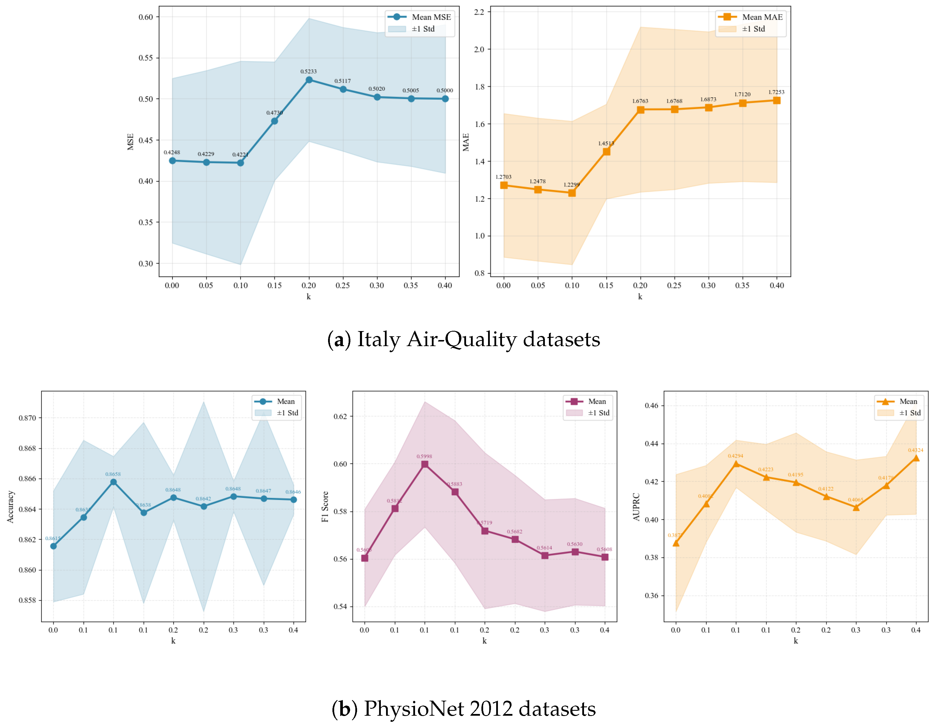
Figure 4a and Figure 4b, respectively, shows the changes in MSE, MAE, Accuracy, F1 score, and AUPRC when k takes different values. Specifically, each indicator represents the average value of that indicator for each imputation model when the k value is the same. It can be seen that when $k=0.1$, the overall effect is the best. Since k represents the proportion of samples to be deleted, the experimental results show that deleting appropriate low-quality samples is beneficial for model learning. However, as the deletion proportion increases, the model performance actually deteriorates. In actual application, we recommend setting k to 0.1 by default. If the result is not satisfactory, adjustments can be made.

4.5. Computational Complexity

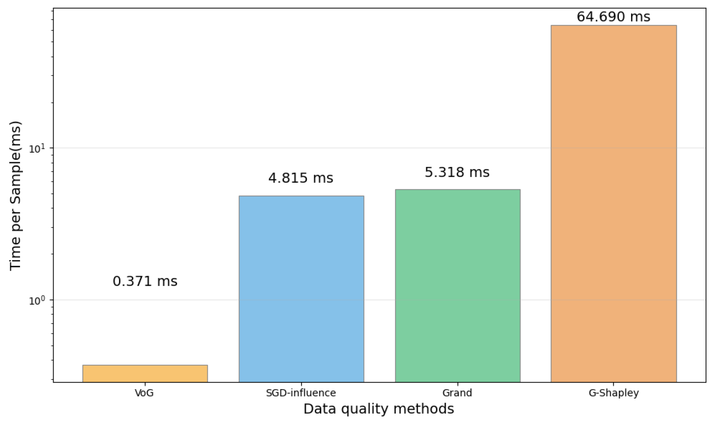
The sample quality assessment algorithm is an important component of the method presented in this paper. Therefore, this experimental analysis discusses its time complexity and execution time. As shown in

Table 10. Time complexity comparison of data quality methods.

Method	Core Mechanism	Time Complexity
VoG	Variance in gradients across training iterations (Equation (5))	$O\left(1\right)$
Grand	Gradient norm of the loss at early training (Equation (4))	$O\left(1\right)$
SGD-influence	The cumulative influence of each sample (Equation (7))	$O\left(n\right)$
G-Shapley	Marginal contribution $v_j^t-v_{j-1}^t$	$O\left(2^n\right)$

, the time complexity of VoG and Grand is $O\left(1\right)$, which is independent of the number of samples; SGD-influence has a linear complexity of $O\left(n\right)$; G-Shapley has the highest time complexity of $O\left(2^n\right)$ because it needs to calculate marginal contribution. Figure 5 also presents the approximate time required for each algorithm to assess a single sample individually. The statistical results are consistent with the analysis. The efficiency of G-Shapley is much lower than that of the other algorithms. It should be noted that in this method, sample quality assessment is independent of downstream model training. Therefore, in practical applications, sample quality can be evaluated offline, which can, to some extent, reduce the time cost of estimating sample quality.

4.6. Understanding Imputed Data Quality

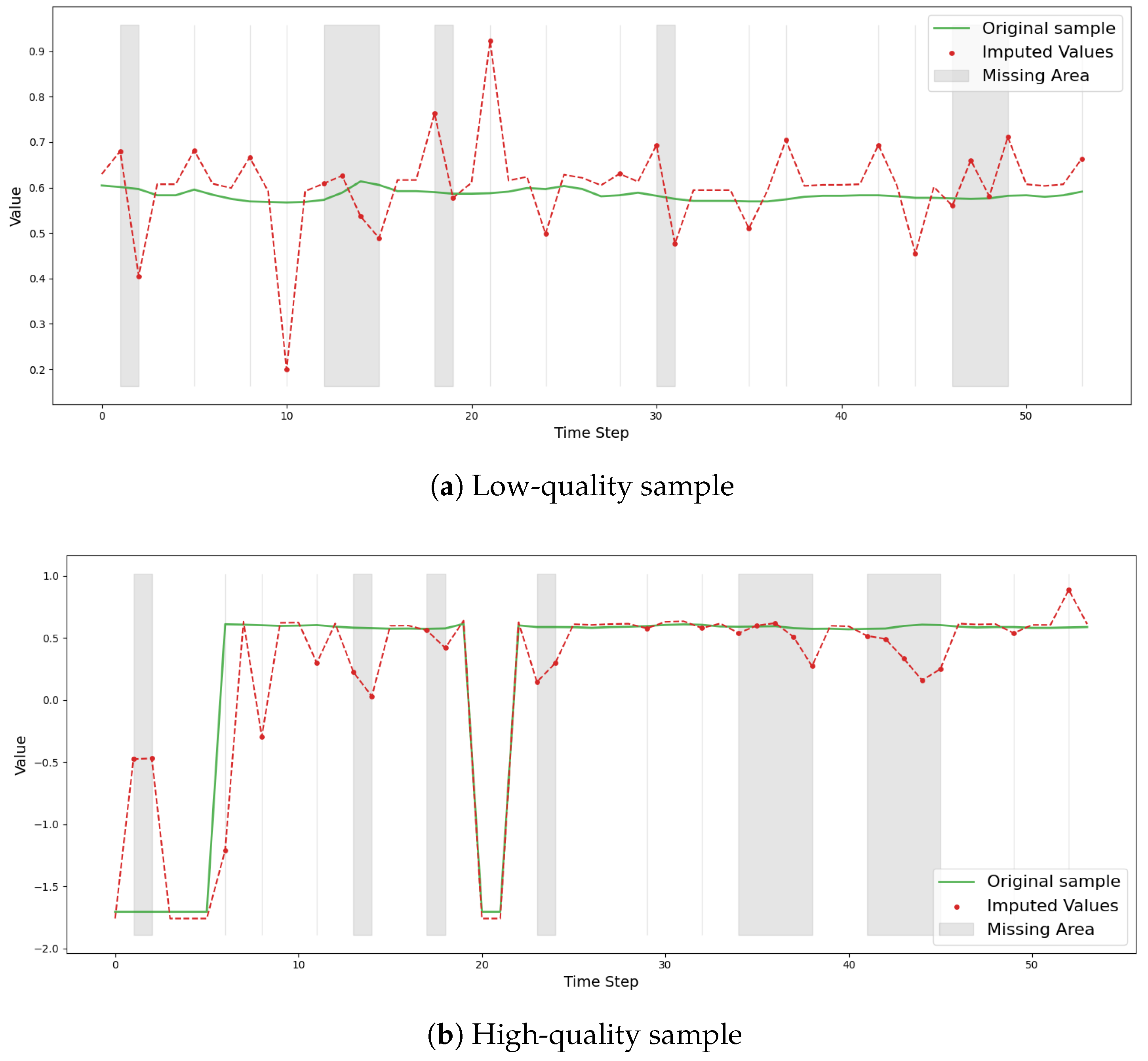
Figure 6 presents two types of samples from Italy Air-Quality datasets. The point-missing pattern marks the positions of missing entries, with a missing rate of $50\%$. Each figure shows the original sample, the missing sample, and the marked missing area and imputed values. The sample (indicated by the dotted line) in Figure 6a has a lower quality (as evaluated by SGD-influence), and Figure 6b shows the high-quality sample (dotted line). In Figure 6a, the trend of the original sample is very gentle, and after interpolation, it shows certain fluctuations, but the gap between the imputed data and the original data is relatively large; in Figure 6b, the sample shows a certain regular pattern of change, and the imputed error of the missing data is lower than that in Figure 6a. However, such observations are difficult to understand or explain the characteristics of low-quality samples. Therefore, this chapter will explore the influencing factors of sample quality from different perspectives.

4.6.1. Relationship Between Sample Quality and Missing Rate

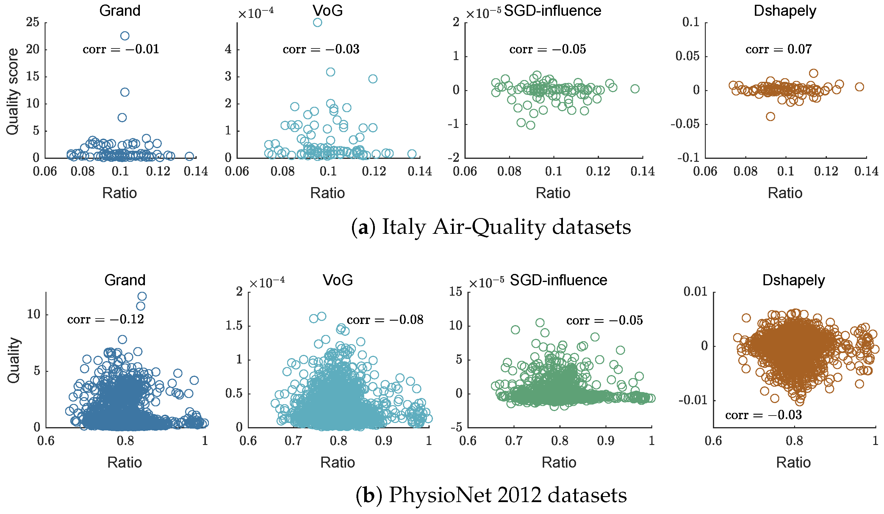
In this experiment, we aim to investigate whether a potential correlation exists between the original missing data rate of a sample and its data quality after imputation. It is important to note that this analysis focuses on the imputed data (i.e., data “repaired” by a specific imputation algorithm), not the original sequences containing missing values. Scatter plots depicting this relationship, along with their corresponding Pearson’s correlation coefficients, are generated for the Italy Air-Quality and PhysioNet 2012 datasets (presented in Figure 7a and Figure 7b, respectively). In experiment, the missing pattern of Italy Air-Quality datasets is point missing with a missing ratio of $10\%$ and imputed by TimesNet.

The results indicate that there is no significant linear correlation between the data quality of an imputed sample and the original missing data rate. This lack of strong correlation can be attributed to the following key reasons: The data quality evaluation algorithms employed in this study evaluate sample quality based on training loss and gradient information. As a result, these algorithms are more sensitive to the difficulty of learning underlying temporal relationships within sequences than to the rate of missing data. This implies that relying solely on missing data rates is insufficient for assessing sample quality. To further clarify the factors influencing variations in sample quality, the following subsection will analyze sample characteristics from the perspective of complex network theory.

4.6.2. Relationship Between Sample Quality and Complex Network Features

The transformation of time series into a complex network for analysis is an emerging technique, pioneered by early work [46]. More recent studies by Qi et al. [47], Cheng et al. [48], and Yang et al. [49] have further explored this approach for tasks including quantifying the complexity of user electricity consumption sequences, time-series classification, and predicting “sleeping beauty” coefficients in scientific publications. Building upon the methodology proposed by Silva et al. [50], this study converts each time-series sample into three distinct graph structures: the Natural Visibility Graph (NVG) [46], the Horizontal Visibility Graph (HVG) [51], and the Quantile Graph (QG) [52]. For each graph, five network features are computed: average degree ($\overline{k}$), average path length ($\overline{d}$), number of communities (S), average clustering coefficient ($\overline{C}$) and modularity (Q). This yields a total of 15 network-derived features per time-series sample.

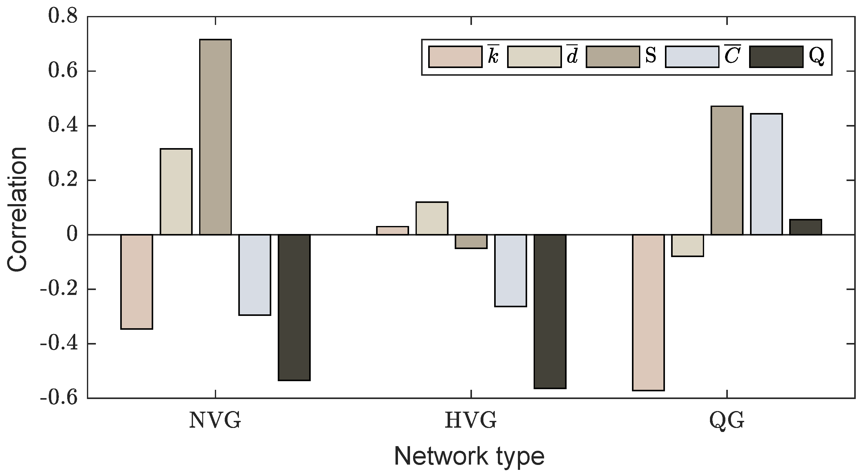
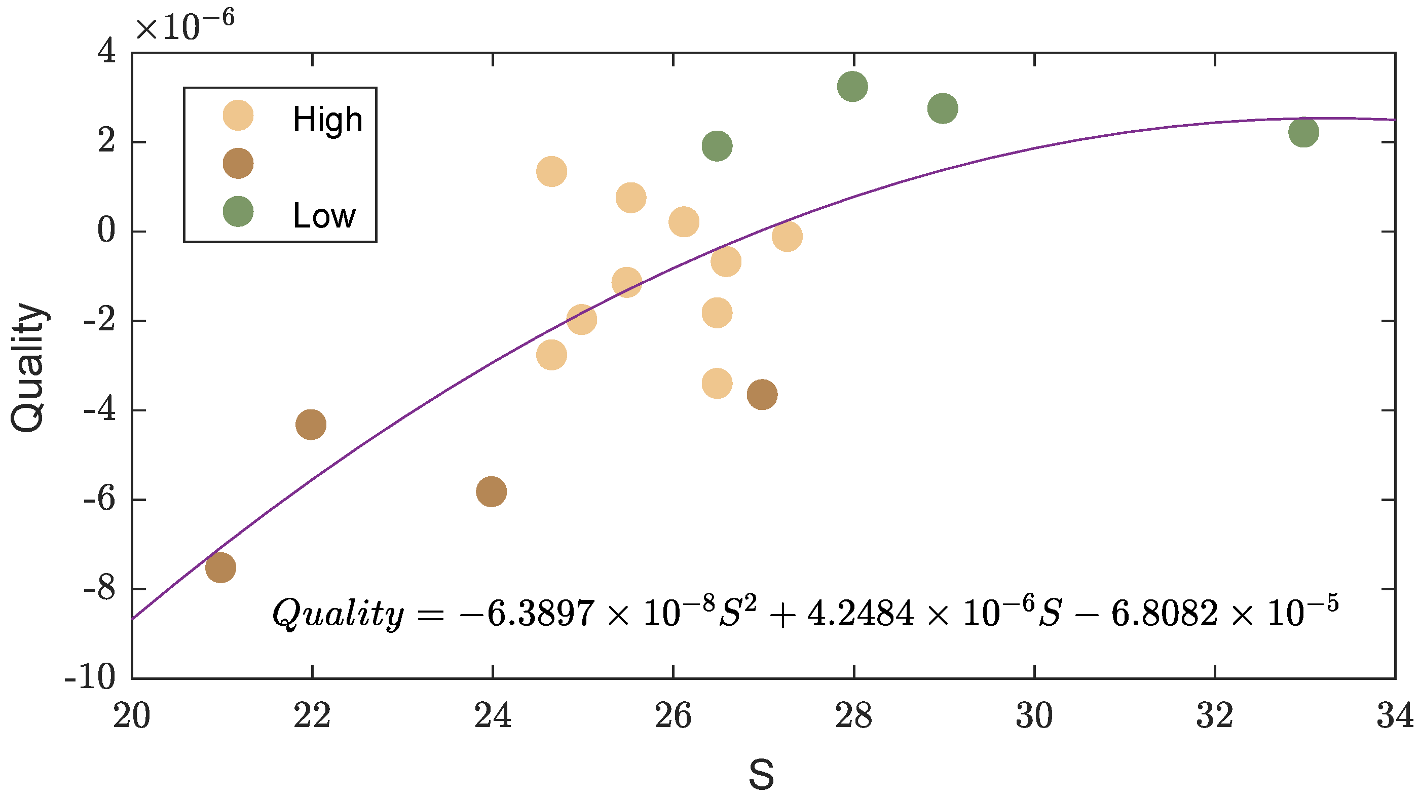
These network features possess inherent physical or structural interpretations, enabling a correlation analysis between the sample quality and these 15 features. For example, When evaluating sample quality using the SGD-influence algorithm, the strongest correlation (Pearson’s $r=0.716$) is observed between sample quality and the number of communities (S) detected in its corresponding NVG (as depicted in Figure 8). For SGD-influence, a higher quality score indicates lower sample quality. Figure 9 illustrates the fitted relationship between the number of communities (S) and sample quality for this specific case. It can be seen that the low-quality samples (indicated by the green dots) are located in the direction with higher scores, while the high-quality samples are in the direction with lower scores. This positive correlation implies that an increase in the number of communities (S) is associated with a decline in sample quality. This relationship can be interpreted as follows: frequent structural changes within a time series, manifesting as an increased number of communities in its graph, may reflect greater temporal complexity. This increased complexity, in turn, can hinder models’ ability to capture underlying dependencies, thereby reducing sample quality (i.e., resulting in a higher SGD-influence score).

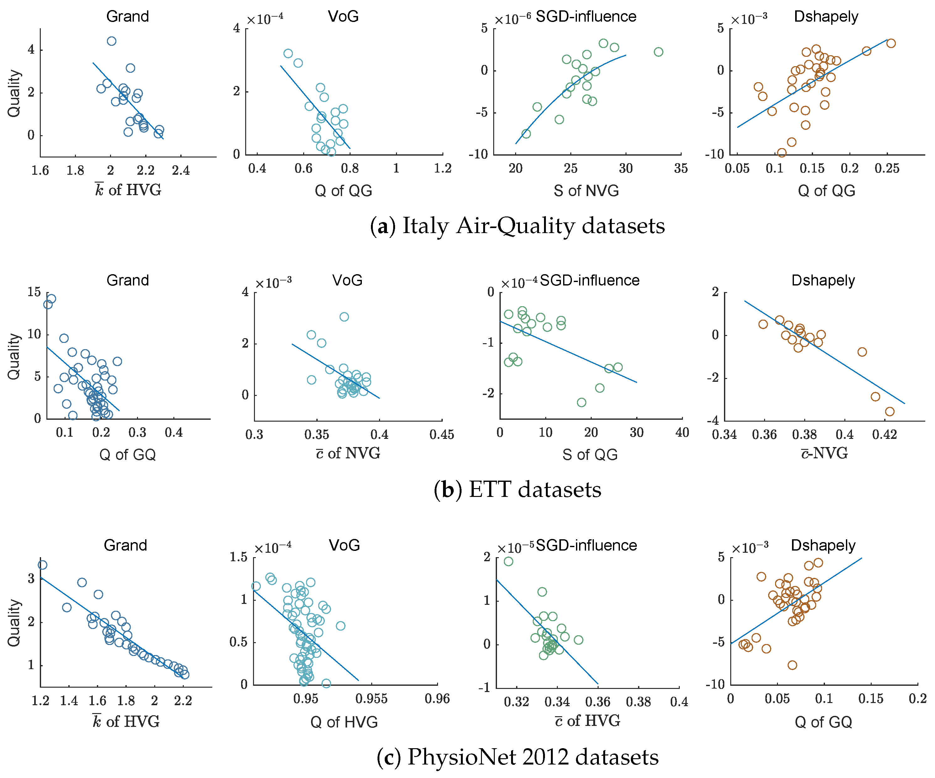
Scatter plots illustrating the strongest correlations between evaluation metrics and network features are shown in Figure 10. In the experiment, the Italy Air-Quality and ETT datasets are set with a missing ratio of $10\%$ and imputed by TimesNet. The results reveal that quality scores generated by different evaluation algorithms indeed exhibit strong correlations with various complex network characteristics. For example, the VoG algorithm shows a strong inverse correlation between data quality and network modularity (Q) for samples from the Italy Air-Quality dataset (see the second plot in Figure 10a); the Grand algorithm demonstrates a strong inverse correlation between data quality and average degree ($\overline{k}$) in the corresponding graph for samples from the PhysioNet 2012 dataset (see the first plot in Figure 10c). These experimental results demonstrate that factors influencing sample quality can be effectively investigated through complex network analysis, offering a novel perspective for understanding data characteristics relevant to model training.

5. Conclusions

In this paper, we propose a methodology that integrates existing imputation algorithms with a subsequent data quality evaluation step to identify and remove low-quality imputed samples, thereby enhancing the performance of imputation algorithms in downstream tasks. Our approach is motivated by the common occurrence of low-quality samples in original time-series datasets. Training imputation models on such data can lead to the generation of poorly imputed samples, which can subsequently impair model training for downstream applications. Through a series of comprehensive experiments, we demonstrate the effectiveness of this approach. For example, MAE can be reduced by up to $38.73\%$ on the Italy Air-Quality dataset, while the AUPRC score can be increased by up to $118.41\%$ on the PhysioNet 2019 dataset. In addition, we also demonstrate the close relationship between data quality and complex-network-derived features of the time series.

However, we only discussed the effectiveness of the method under MCAR scenarios and did not start the experiment under MAR and MNAR. This is a limitation of this study. Furthermore, the method proposed in this paper does not utilize data quality to optimize the design of the imputation model instead of directly deleting some low-quality samples. Therefore, in the future, we will attempt to design an imputation model based on data quality feedback to directly generate high-quality imputed time series and conduct experiments in challenging scenarios such as MAR and MNAR.

References

1. Fang, W.; Zhuo, W.; Yan, J.; Song, Y.; Jiang, D.; Zhou, T. Attention meets long short-term memory: A deep learning network for traffic flow forecasting. Phys. A Stat. Mech. Its Appl. 2022, 587, 126485. [Google Scholar] [CrossRef]
2. Zhang, W.; Yang, L.; Geng, S.; Hong, S. Self-Supervised Time Series Representation Learning via Cross Reconstruction Transformer. IEEE Trans. Neural Netw. Learn. Syst. 2024, 35, 16129–16138. [Google Scholar] [CrossRef] [PubMed]
3. Liang, Y.; Xia, Y.; Ke, S.; Wang, Y.; Wen, Q.; Zhang, J.; Zheng, Y.; Zimmermann, R. Airformer: Predicting nationwide air quality in china with transformers. In Proceedings of the AAAI Conference on Artificial Intelligence; AAAI: Washington, DC, USA, 2023; Volume 37, pp. 14329–14337. [Google Scholar]
4. Du, W.; Wang, J.; Qian, L.; Yang, Y.; Liu, F.; Wang, Z.; Ibrahim, Z.; Liu, H.; Zhao, Z.; Zhou, Y.; et al. TSI-Bench: Benchmarking Time Series Imputation. arXiv 2024, arXiv:2406.12747. [Google Scholar]
5. Wang, J.; Du, W.; Cao, W.; Zhang, K.; Wang, W.; Liang, Y.; Wen, Q. Deep Learning for Multivariate Time Series Imputation: A Survey. arXiv 2024, arXiv:2402.04059. [Google Scholar]
6. Miao, X.; Wu, Y.; Chen, L.; Gao, Y.; Yin, J. An Experimental Survey of Missing Data Imputation Algorithms. IEEE Trans. Knowl. Data Eng. 2023, 35, 6630–6650. [Google Scholar] [CrossRef]
7. Huang, F.; Wang, J.; Yi, P.; Peng, J.; Xiong, X.; Liu, Y. SCSQ: A sample cooperation optimization method with sample quality for recurrent neural networks. Inf. Sci. 2024, 674, 120730. [Google Scholar] [CrossRef]
8. RUBIN, D.B. Inference and missing data. Biometrika 1976, 63, 581–592. [Google Scholar] [CrossRef]
9. García-Laencina, P.J.; Sancho-Gómez, J.L.; Figueiras-Vidal, A.R. Pattern classification with missing data: A review. Neural Comput. Appl. 2010, 19, 263–282. [Google Scholar]
10. Batista, G.E.A.P.A.; Monard, M.C. An analysis of four missing data treatment methods for supervised learning. Appl. Artif. Intell. 2003, 17, 519–533. [Google Scholar] [CrossRef]
11. Twala, B.; Cartwright, M.; Shepperd, M. Comparison of various methods for handling incomplete data in software engineering databases. In Proceedings of the International Symposium on Empirical Software Engineering; IEEE: Piscataway, NJ, USA, 2005; pp. 234–239. [Google Scholar]
12. Jerez, J.M.; Molina, I.; García-Laencina, P.J.; Alba, E.; Ribelles, N.; Martín, M.; Franco, L. Missing data imputation using statistical and machine learning methods in a real breast cancer problem. Artif. Intell. Med. 2010, 50, 105–115. [Google Scholar] [CrossRef] [PubMed]
13. Hastie, T.; Mazumder, R.; Lee, J.; Zadeh, R. Matrix Completion and Low-Rank SVD via Fast Alternating Least Squares. J. Mach. Learn. Res. 2014, 16, 3367–3402. [Google Scholar]
14. Mazumder, R.; Hastie, T.; Tibshirani, R. Spectral Regularization Algorithms for Learning Large Incomplete Matrices. J. Mach. Learn. Res. JMLR 2010, 11, 2287–2322. [Google Scholar] [PubMed]
15. Antonenko, E.; Carreño, A.; Read, J. Autoreplicative random forests with applications to missing value imputation. Mach. Learn. 2024, 113, 7617–7643. [Google Scholar] [CrossRef]
16. McCoy, J.T.; Kroon, S.; Auret, L. Variational Autoencoders for Missing Data Imputation with Application to a Simulated Milling Circuit. IFAC-PapersOnLine 2018, 51, 141–146. [Google Scholar] [CrossRef]
17. Fortuin, V.; Baranchuk, D.; Rätsch, G.; Mandt, S. Gp-vae: Deep probabilistic time series imputation. In Proceedings of the International Conference on Artificial Intelligence and Statistics; PMLR: New York, NY, USA, 2020; pp. 1651–1661. [Google Scholar]
18. Mulyadi, A.W.; Jun, E.; Suk, H.I. Uncertainty-Aware Variational-Recurrent Imputation Network for Clinical Time Series. IEEE Trans. Cybern. 2022, 52, 9684–9694. [Google Scholar] [CrossRef] [PubMed]
19. Luo, Y.; Cai, X.; Zhang, Y.; Xu, J.; Yuan, X. Multivariate time series imputation with generative adversarial networks. In Proceedings of the 32nd International Conference on Neural Information Processing Systems, NIPS’18; Curran Associates, Inc.: Red Hook, NY, USA, 2018; pp. 1603–1614. [Google Scholar]
20. Luo, Y.; Zhang, Y.; Cai, X.; Yuan, X. E2GAN: End-to-End Generative Adversarial Network for Multivariate Time Series Imputation. In Proceedings of the Twenty-Eighth International Joint Conference on Artificial Intelligence, IJCAI-19; International Joint Conferences on Artificial Intelligence Organization: Macao, China, 2019; pp. 3094–3100. [Google Scholar] [CrossRef] [PubMed]
21. Tashiro, Y.; Song, J.; Song, Y.; Ermon, S. Csdi: Conditional score-based diffusion models for probabilistic time series imputation. Adv. Neural Inf. Process. Syst. 2021, 34, 24804–24816. [Google Scholar]
22. Alcaraz, J.L.; Strodthoff, N. Diffusion-based Time Series Imputation and Forecasting with Structured State Space Models. arXiv 2022, arXiv:2208.09399. [Google Scholar]
23. Chen, Y.; Deng, W.; Fang, S.; Li, F.; Yang, N.T.; Zhang, Y.; Rasul, K.; Zhe, S.; Schneider, A.; Nevmyvaka, Y. Provably convergent Schrödinger bridge with applications to probabilistic time series imputation. In Proceedings of the International Conference on Machine Learning; PMLR: New York, NY, USA, 2023; pp. 4485–4513. [Google Scholar]
24. Wu, H.; Hu, T.; Liu, Y.; Zhou, H.; Wang, J.; Long, M. TimesNet: Temporal 2D-Variation Modeling for General Time Series Analysis. In Proceedings of the International Conference on Learning Representations; Curran Associates, Inc.: Red Hook, NY, USA, 2023. [Google Scholar]
25. Che, Z.; Purushotham, S.; Cho, K.; Sontag, D.; Liu, Y. Recurrent neural networks for multivariate time series with missing values. Sci. Rep. 2018, 8, 6085. [Google Scholar] [CrossRef] [PubMed]
26. Cao, W.; Wang, D.; Li, J.; Zhou, H.; Li, Y.; Li, L. BRITS: Bidirectional recurrent imputation for time series. In Proceedings of the 32nd International Conference on Neural Information Processing Systems; Curran Associates, Inc.: Red Hook, NY, USA, 2018; pp. 6776–6786. [Google Scholar]
27. Yoon, J.; Zame, W.R.; van der Schaar, M. Estimating missing data in temporal data streams using multi-directional recurrent neural networks. IEEE Trans. Biomed. Eng. 2018, 66, 1477–1490. [Google Scholar] [CrossRef] [PubMed]
28. Bai, S.; Kolter, J.Z.; Koltun, V. An empirical evaluation of generic convolutional and recurrent networks for sequence modeling. arXiv 2018, arXiv:1803.01271. [Google Scholar]
29. Wang, H.; Peng, J.; Huang, F.; Wang, J.; Chen, J.; Xiao, Y. Micn: Multi-scale local and global context modeling for long-term series forecasting. In Proceedings of the Eleventh International Conference on Learning Representations; Curran Associates, Inc.: Red Hook, NY, USA, 2023. [Google Scholar]
30. Cao, D.; Wang, Y.; Duan, J.; Zhang, C.; Zhu, X.; Huang, C.; Tong, Y.; Xu, B.; Bai, J.; Tong, J.; et al. Spectral temporal graph neural network for multivariate time-series forecasting. Adv. Neural Inf. Process. Syst. 2020, 33, 17766–17778. [Google Scholar]
31. Cini, A.; Marisca, I.; Alippi, C. Filling the G_ap_s: Multivariate Time Series Imputation by Graph Neural Networks. In Proceedings of the International Conference on Learning Representations; Curran Associates, Inc.: Red Hook, NY, USA, 2022. [Google Scholar]
32. Marisca, I.; Cini, A.; Alippi, C. Learning to reconstruct missing data from spatiotemporal graphs with sparse observations. Adv. Neural Inf. Process. Syst. 2022, 35, 32069–32082. [Google Scholar] [CrossRef]
33. Zhou, H.; Zhang, S.; Peng, J.; Zhang, S.; Li, J.; Xiong, H.; Zhang, W. Informer: Beyond efficient transformer for long sequence time-series forecasting. In Proceedings of the AAAI Conference on Artificial Intelligence; AAAI: Washington, DC, USA, 2021. [Google Scholar]
34. Bansal, P.; Deshpande, P.; Sarawagi, S. Missing value imputation on multidimensional time series. Proc. VLDB Endow. 2021, 14, 2533–2545. [Google Scholar] [CrossRef]
35. Du, W.; Côté, D.; Liu, Y. Saits: Self-attention-based imputation for time series. Expert Syst. Appl. 2023, 219, 119619. [Google Scholar]
36. Ng, A. A Chat with Andrew on MLOps: From Model-Centric to Data-Centric AI. Available online: https://www.youtube.com/watch?v=06-AZXmwHjo (accessed on 1 July 2026).
37. Zhou, Y.; Tu, F.; Sha, K.; Ding, J.; Chen, H. A Survey on Data Quality Dimensions and Tools for Machine Learning Invited Paper. In Proceedings of the 2024 IEEE International Conference on Artificial Intelligence Testing (AITest); IEEE: Piscataway, NJ, USA, 2024; pp. 120–131. [Google Scholar] [CrossRef]
38. Koh, P.W.; Liang, P. Understanding Black-Box Predictions via Influence Functions. In Proceedings of the 34th International Conference on Machine Learning, ICML’17; PMLR: New York, NY, USA, 2017; Volume 70, pp. 1885–1894. [Google Scholar]
39. Hara, S.; Nitanda, A.; Maehara, T. Data cleansing for models trained with SGD. In Proceedings of the 33rd International Conference on Neural Information Processing Systems; Curran Associates, Inc.: Red Hook, NY, USA, 2019. [Google Scholar]
40. Jia, R.; Wu, F.; Sun, X.; Xu, J.; Dao, D.; Kailkhura, B.; Zhang, C.; Li, B.; Song, D. Scalability vs. Utility: Do We Have to Sacrifice One for the Other in Data Importance Quantification? In Proceedings of the 2021 IEEE/CVF Conference on Computer Vision and Pattern Recognition (CVPR); IEEE: Piscataway, NJ, USA, 2021; pp. 8235–8243. [Google Scholar]
41. Paul, M.; Ganguli, S.; Dziugaite, G.K. Deep learning on a data diet: Finding important examples early in training. Adv. Neural Inf. Process. Syst. 2021, 34, 20596–20607. [Google Scholar]
42. Agarwal, C.; D’souza, D.; Hooker, S. Estimating example difficulty using variance of gradients. In Proceedings of the IEEE/CVF Conference on Computer Vision and Pattern Recognition; IEEE: Piscataway, NJ, USA, 2022; pp. 10368–10378. [Google Scholar]
43. Ghorbani, A.; Zou, J. Data shapley: Equitable valuation of data for machine learning. In Proceedings of the International Conference on Machine Learning; PMLR: New York, NY, USA, 2019; pp. 2242–2251. [Google Scholar]
44. Miao, X.; Wu, Y.; Wang, J.; Gao, Y.; Mao, X.; Yin, J. Generative Semi-supervised Learning for Multivariate Time Series Imputation. In Proceedings of the AAAI Conference on Artificial Intelligence; AAAI: Washington, DC, USA, 2021; Volume 35, pp. 8983–8991. [Google Scholar] [CrossRef]
45. Boyd, K.; Eng, K.H.; Page, C.D. Area under the Precision-Recall Curve: Point Estimates and Confidence Intervals. In Proceedings of the Machine Learning and Knowledge Discovery in Databases; Blockeel, H., Kersting, K., Nijssen, S., Železný, F., Eds.; Springer: Berlin/Heidelberg, Germany, 2013; pp. 451–466. [Google Scholar]
46. Lacasa, L.; Luque, B.; Ballesteros, F.; Luque, J.; Nuño, J.C. From time series to complex networks: The visibility graph. Proc. Natl. Acad. Sci. USA 2008, 105, 4972–4975. [Google Scholar] [CrossRef] [PubMed]
47. Qi, M.; Mei, L.; Li, Z.; Yan, L.; Wang, Z.; Ju, P. Revealing the Complexity of Load Fluctuations for Electricity Consumers Using MLP-HVG. In Proceedings of the 2023 IEEE Power and Energy Society General Meeting (PESGM); IEEE: Piscataway, NJ, USA, 2023; pp. 1–5. [Google Scholar] [CrossRef]
48. Cheng, L.; Zhu, P.; Sun, W.; Han, Z.; Tang, K.; Cui, X. Time series classification by Euclidean distance-based visibility graph. Phys. A Stat. Mech. Its Appl. 2023, 625, 129010. [Google Scholar] [CrossRef]
49. Yang, N.; Huang, F.; Zhao, S.; Li, S.; Hu, W. Predicting Sleeping Beauty Coefficients Based on ts2net Model. Data Anal. Knowl. Discov. 2024, 8, 72–82. [Google Scholar] [CrossRef]
50. Silva, V.F.; Silva, M.E.; Ribeiro, P.; Silva, F. Novel features for time series analysis: A complex networks approach. Data Min. Knowl. Discov. 2022, 36, 1062–1101. [Google Scholar] [CrossRef]
51. Luque, B.; Lacasa, L.; Ballesteros, F.; Luque, J. Horizontal visibility graphs: Exact results for random time series. Phys. Rev. E—Stat. Nonlinear Soft Matter Phys. 2009, 80, 046103. [Google Scholar] [CrossRef]
52. Campanharo, A.S.; Sirer, M.I.; Malmgren, R.D.; Ramos, F.M.; Amaral, L.A.N. Duality between time series and networks. PLoS ONE 2011, 6, e23378. [Google Scholar] [CrossRef] [PubMed]
Figure 1. Example of how bad imputation samples result in a bigger loss.
Applsci 16 06837 g001
Figure 2. Illustration of quality difference.
Applsci 16 06837 g002
Figure 3. Workflow of proposed method.
Applsci 16 06837 g003
Figure 4. The changes in the indicator when k takes different values.
Applsci 16 06837 g004
Figure 5. Evaluation time.
Applsci 16 06837 g005
Figure 6. Sample visualization.
Applsci 16 06837 g006
Figure 7. Scatter plot of sample score.
Applsci 16 06837 g007
Figure 8. Correlation between sample quality and complex features in NVG graph.
Applsci 16 06837 g008
Figure 9. Scatter plot of SGD-influence on Italy Air-Quality.
Applsci 16 06837 g009
Figure 10. Scatter plot between sample quality and complex network features.
Applsci 16 06837 g010