A Lightweight 1D-CNN for Bark and Howl Classification from Raw Audio Waveforms Under Controlled Additive Noise

Featured Application

This study supports lightweight dog vocalization monitoring systems that classify Bark and Howl directly from raw waveforms. The reported evidence concerns recording-level performance without added synthetic noise and under controlled additive-noise conditions; subject-independent field validation remains necessary.

Abstract

Automatic classification of dog vocalizations can support bioacoustic monitoring and animal welfare, but many systems require spectral or cepstral preprocessing. This study evaluates a lightweight one-dimensional convolutional neural network (1D-CNN) for Bark and Howl classification directly from raw waveforms under controlled additive noise. The dataset comprised 46 Bark and 57 Howl recordings. Audio was converted to mono, resampled to 16 kHz, and standardized to 2.0 s. The network contains 7130 trainable parameters, occupies 27.85 KB with 32-bit weights, and requires 18.35 MFLOPs. The complete five-fold cross-validation procedure was repeated ten times with independently generated run-specific seeds and newly shuffled partitions. Under the no-added-noise condition, mean accuracy was 93.40 ± 2.62%, and macro F1-score was 93.20 ± 2.75%. Performance remained within run-to-run variability between 30 and 5 dB SNR for Gaussian and uniform additive noise, whereas mean accuracy decreased to 79.42% at 0 dB. In the seed-42 reference ablation, removing noise augmentation preserved no-added-noise accuracy but reduced 5 dB accuracy by approximately 20 percentage points. The findings provide preliminary recording-level evidence for efficient Bark and Howl classification under controlled conditions. Generalization to unseen dogs and field recordings remains unverified.

1. Introduction

Animal vocalizations provide information about behavior, communication, and environmental interaction. Automated acoustic analysis is therefore relevant to bioacoustics, conservation monitoring, animal welfare, and precision animal monitoring [1,2,3,4,5]. Manual inspection of audio archives is slow and subjective. This limitation motivates automatic methods that can identify relevant vocal events with limited human intervention.

Dog vocalizations are of practical interest because domestic dogs communicate with humans and other animals through diverse acoustic patterns. Barking is often short and repetitive, whereas howling is generally longer and more sustained. Prior studies have shown that dog vocal signals contain context-related and individual-related acoustic information [6,7]. Consequently, a recording-level classifier may learn both vocalization-type characteristics and subject-specific cues when individual identities are not controlled.

Traditional animal sound analysis frequently relies on handcrafted or spectral features before classification. Yeo et al. used zero-crossing rate and Mel-frequency cepstral coefficients for dog voice identification [8]. Bishop et al. combined audio-specific features with machine learning for livestock vocalization classification [9]. Nunes et al. used audio-based artificial intelligence for horse foraging behavior detection [10], and Tsai and Huang incorporated spectrogram-based analysis into a pet sentiment system [11]. These studies demonstrate the utility of acoustic learning systems, but they also illustrate the dependence of many pipelines on feature engineering or spectral transformations.

Deep CNNs can process time–frequency representations effectively, and standard image CNNs can provide strong baselines for spectrogram classification [12]. However, spectral pipelines introduce choices such as window length, hop size, frequency resolution, coefficient count, and image resizing. Raw-waveform learning offers a more direct alternative by learning temporal filters from one-dimensional samples [13,14]. Compact audio architectures are also well established in small-footprint tasks, including temporal convolution, broadcasted residual learning, time-channel separable convolution, and compressed raw-waveform networks [15,16,17,18]. Therefore, the contribution of the present model is application-specific and incremental rather than a new general convolutional paradigm.

Karaaslan et al. developed a fully automatic dog vocalization analysis system that segmented dog sounds and evaluated CNN classifiers using Short-Time Fourier Transform (STFT), Mel spectrogram, Mel-frequency cepstral coefficients (MFCCs), and linear-frequency cepstral coefficients (LFCCs) [1]. The highest reported overall accuracy among the feature-based CNN configurations considered in that study was 90.00% [1]. Their work established a useful reference for the Bark and Howl task, but the reported models used large two-dimensional backbones and feature-dependent preprocessing.

The present study investigates whether a highly compact 1D-CNN can classify Bark and Howl directly from fixed-length raw waveforms while maintaining stable performance under analytically controlled additive corruption. Gaussian and uniform noise are used as reproducible stressors at predefined signal-to-noise ratio (SNR) levels. The study does not claim general robustness to environmental sound, reverberation, overlapping sources, microphone variability, or field-recorded conditions. This restricted interpretation is important because controlled additive noise does not reproduce the full acoustic variability of real monitoring environments. Reliability is assessed through ten repetitions of five-fold cross-validation, and a targeted ablation analysis examines the roles of noise augmentation, batch normalization, dropout, and input duration.

The main contributions are as follows:

• A 7130-parameter 1D-CNN is evaluated for Bark and Howl classification directly from 2.0 s raw waveform segments.
• The full five-fold cross-validation procedure is repeated ten times to quantify variability across dataset partitions and stochastic training runs.
• Controlled Gaussian and uniform additive-noise performance is evaluated from 30 to 0 dB SNR, including an intermediate 15 dB condition that was deliberately excluded from training.
• A seed-42 reference ablation study evaluates noise augmentation, batch normalization, dropout, and 1 s, 2 s, and 3 s input durations.
• Parameter count, model size, FLOPs, inference time, and contextual comparisons with feature-based and compact audio architectures are reported.

The remainder of this paper is organized as follows. Section 2 describes the dataset, waveform processing, controlled noise augmentation, model, repeated evaluation protocol, ablation design, and computational analysis. Section 3 presents the results. Section 4 discusses their interpretation and limitations. Section 5 concludes the paper.

2. Materials and Methods

2.1. Dataset

This study used the dog vocalization subset reported by Karaaslan et al. [1]. The binary classification task contains 46 Bark recordings and 57 Howl recordings, giving 103 labeled samples in total. Cat recordings and other animal sounds were excluded. No new animal recordings were collected; the experiments constitute a secondary computational analysis of the openly available dataset.

The public metadata do not provide individual dog identifiers or a recording-to-subject mapping. The number of unique dogs represented by the 103 recordings therefore cannot be determined. No attempt was made to infer identity from file names or acoustic similarity. Consequently, all reported partitions operate at the recording level, and subject-independent generalization cannot be established.

Table 1. Dataset composition used for binary Bark and Howl classification.

Class	Number of Samples	Percentage (%)
Bark	46	44.66
Howl	57	55.34
Total	103	100

summarizes the class distribution used for the binary Bark and Howl classification task.

2.2. Raw Waveform Standardization

Each audio file was loaded as a waveform signal. Multichannel recordings were converted to mono by averaging the channels. Signals were resampled to 16 kHz when required. The waveforms were not normalized on a per-record basis using peak amplitude, root-mean-square (RMS) amplitude, or z-score normalization. The decoded floating-point samples retained their original relative amplitude differences within the nominal digital-audio range. No handcrafted spectral representation was generated for the proposed model.

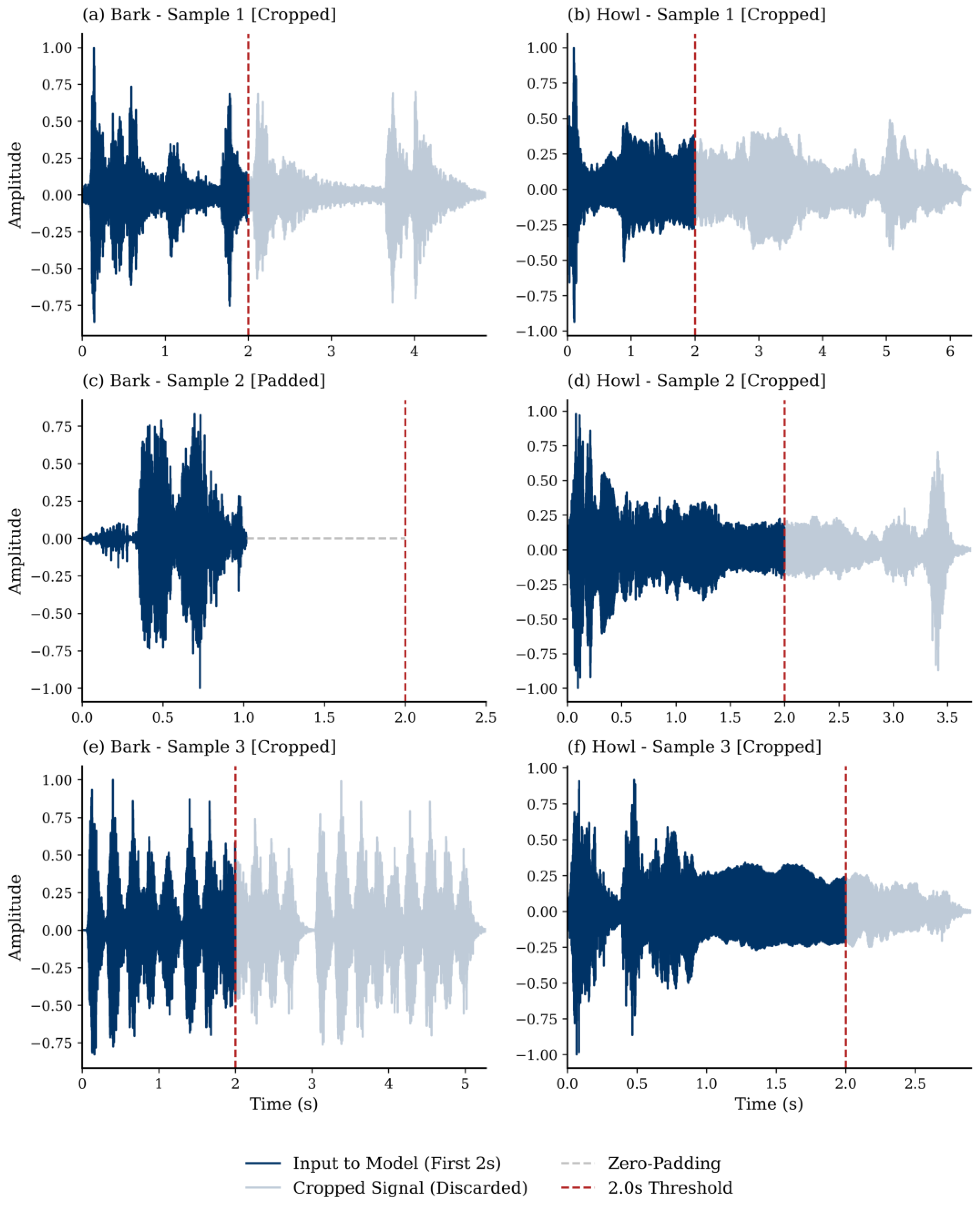
Each waveform was standardized to 2.0 s. At 16 kHz, this duration corresponds to 32,000 samples. Longer recordings were truncated to the first 32,000 samples, and shorter recordings were zero-padded at the end. The resulting input tensor had size B × 1 × 32,000, where B denotes batch size. Figure 1 illustrates representative Bark and Howl examples.

The target input length was computed using Equation (1).

L = f_s T,

(1)

where L is the target number of samples, f_s is the sampling rate, and T is the segment duration. In this study, f_s = 16,000 Hz and T = 2.0 s, giving L = 32,000.

Let x = {x₁, x₂,…, xN} denote an input waveform with N samples. The standardized waveform, x_std, was obtained using Equation (2), which retains the first 2.0 s of longer recordings and appends zeros to shorter recordings.

x_std[n] = x[n], 1 ≤ n ≤ min(N,L); x_std[n] = 0, N < n ≤ L,

(2)

2.3. Controlled Additive-Noise Augmentation

Online noise augmentation was applied during training. Audio augmentation can improve generalization in environmental and animal sound classification when labeled recordings are limited [19,20]. For each mini-batch, additive noise was applied with probability of 0.95. When augmentation was selected, the noise type was sampled as Gaussian or uniform additive noise. The training SNR was selected from 30, 20, 10, 5, and 0 dB. The 15 dB condition was deliberately excluded from training and used only as an intermediate unseen SNR level during evaluation.

Gaussian and uniform noise were selected as analytically defined perturbations whose power could be controlled directly through SNR. They were not intended to reproduce the spectral and temporal complexity of real environments. The corresponding experiments should therefore be interpreted as controlled additive-noise stress tests rather than field-noise validation.

For an unmodified waveform (x) with length (L), signal power (Px) was computed using Equation (3). The scaling followed the standard power-ratio definition of SNR [21].

P_x = (1/L) ∑_n ₌ ₁ᴸ x_n²,

(3)

The target SNR, in decibels, was converted to a linear ratio using Equation (4).

SNR_lin = 10^(SNRdB/10),

(4)

The required noise power, Pη, was then computed using Equation (5).

Pη = P_x/SNR_lin,

(5)

The corrupted waveform was defined by Equation (6).

x̃ = x + η,

(6)

For Gaussian augmentation, η was sampled from a zero-mean normal distribution and scaled to the target power. For uniform augmentation, an initial vector, u, was sampled from U(−1,1) and rescaled using Equation (7). No clipping or post-addition normalization was applied after either corruption process.

η_u = u √(Pη/P_u), P_u = (1/L) ∑_n = ₁^L u_n².

(7)

The second branch is reported as uniform additive noise because it was generated from a uniform random distribution rather than from recorded physiological or environmental signals.

2.4. Proposed 1D-CNN Architecture

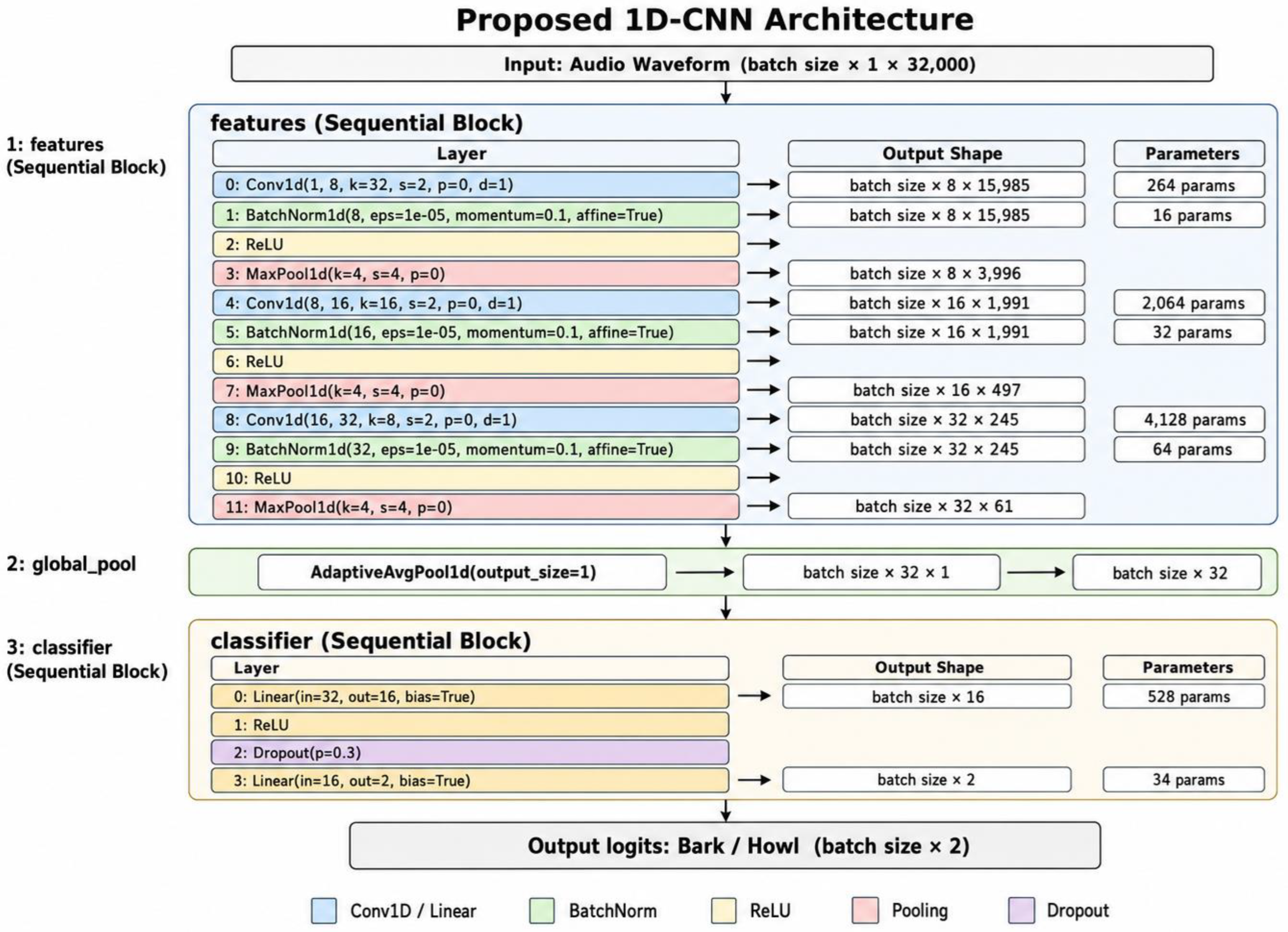
The proposed architecture is a compact one-dimensional CNN. CNNs learn hierarchical representations by applying trainable local filters to structured inputs [22]. Here, the filters operate along the temporal axis of the raw waveform. The feature extractor contains three Conv1D blocks. Each block includes convolution, batch normalization, ReLU activation, and max pooling. Batch normalization was used to stabilize optimization [23], and ReLU was selected as a computationally simple nonlinear activation [24,25].

After the third block, adaptive average pooling compresses the temporal dimension to one and yields a 32-dimensional feature vector. The classifier maps this vector to 16 hidden units, applies ReLU and dropout, and produces two logits. Adaptive average pooling limits the size of the fully connected classifier [26], and dropout provides regularization [27]. Figure 2 presents the architecture, and

Table 2. Layer-wise configuration of the proposed 1D-CNN architecture.

Layer	Input Shape	Output Shape	Kernel/Setting	Trainable Parameters
Conv1D 1	1 × 32,000	8 × 15,985	k = 32, s = 2, p = 0	264
BatchNorm1D 1	8 × 15,985	8 × 15,985	-	16
MaxPool1D 1	8 × 15,985	8 × 3996	k = 4, s = 4	0
Conv1D 2	8 × 3996	16 × 1991	k = 16, s = 2, p = 0	2064
BatchNorm1D 2	16 × 1991	16 × 1991	-	32
MaxPool1D 2	16 × 1991	16 × 497	k = 4, s = 4	0
Conv1D 3	16 × 497	32 × 245	k = 8, s = 2, p = 0	4128
BatchNorm1D 3	32 × 245	32 × 245	-	64
MaxPool1D 3	32 × 245	32 × 61	k = 4, s = 4	0
AdaptiveAvgPool1D	32 × 61	32 × 1	Output length = 1	0
Linear 1	32	16	-	528
Dropout	16	16	p = 0.3	0
Linear 2	16	2	-	34
Total	-	-	-	7130

lists the layer-wise configuration.

For a one-dimensional convolutional layer, output length was computed using Equation (8), following standard convolution arithmetic [28].

L_out = floor((L_in + 2p − d(k − 1) − 1)/s + 1),

(8)

where L_in is input length, p is padding, d is dilation, k is kernel size, and s is stride. Equation (8) was used to verify the dimensions in Table 2.

2.5. Training Configuration

The model was implemented in Python 3.13.5 using PyTorch 2.9.0+cu126 (https://pytorch.org/) [29] and NumPy 2.2.6 (https://numpy.org/). GPU acceleration was performed using CUDA 12.6 through the CUDA-enabled PyTorch backend and cuDNN 9.10.2 when available. The model was optimized with Adam [30]. The learning rate was 0.001, the batch size was 16, and each fold was trained for 200 epochs with cross-entropy loss. A separate Softmax layer was not used, because the loss receives logits directly. The architecture and hyperparameters were selected empirically during preliminary development experiments; no exhaustive or systematic grid search was performed. All settings were fixed before the final repeated evaluation. No separate validation subset was used. The epoch count was fixed in advance, and no information from the held-out test folds was used for hyperparameter adjustment, early stopping, or model selection.

Within each repetition, a run-specific seed controlled Python, NumPy, PyTorch, stochastic augmentation, and the shuffled five-fold partition. c seeds were also set when a GPU was available, and deterministic cuDNN behavior was enabled. Experiments were performed on a desktop computer equipped with an Intel Core i3-12100F CPU at 3.30 GHz (Intel Corporation, Santa Clara, CA, USA), 8 GB RAM, and an NVIDIA GeForce RTX 3060 GPU with 12 GB memory (NVIDIA Corporation, Santa Clara, CA, USA). Training used the GPU, whereas waveform loading and auxiliary processing used the CPU.

2.6. Repeated Five-Fold Cross-Validation

Repeated five-fold cross-validation was used as the resampling framework [31]. The complete procedure was repeated ten times to assess sensitivity to dataset partitioning and stochastic training. For each repetition, an independently generated run-specific seed produced a newly shuffled five-fold partition and controlled the stochastic training operations. Four folds were used for training, and one fold for testing. The model was reinitialized at the beginning of every fold, and each recording was evaluated once per repetition.

After training, each model was first evaluated on the held-out fold without added synthetic noise. The same model was then tested after Gaussian or uniform additive corruption at 30, 20, 15, 10, 5, and 0 dB SNR. Predictions from the five test folds were pooled within each repetition before the performance metrics were calculated. The ten repetition-level metric values were summarized using their mean, sample standard deviation, and a 95% confidence interval for the mean based on Student’s t distribution with nine degrees of freedom.

The confidence intervals summarize the observed run-to-run variation across the ten repeated procedures. Because cross-validation estimates are dependent through overlapping training sets, these intervals should not be interpreted as unbiased population-level generalization intervals [32]. The confusion matrix was row-normalized and used only to summarize the aggregated class-level error pattern across repetitions.

Individual dog identifiers were unavailable. Consequently, the folds were generated at the recording level, and Leave-One-Subject-Out or other subject-disjoint validation could not be performed.

2.7. Ablation Analysis

A targeted ablation study was conducted using the seed-42 reference five-fold experiment. The full model was compared with variants trained without noise augmentation, without batch normalization, and without dropout. Input-duration variants of 1.0 s and 3.0 s were also evaluated against the 2.0 s reference. All configurations used the same seed-42 folds, identical noisy test realizations, and the same training settings unless the indicated factor was changed. No-added-noise accuracy and accuracy under 5 dB Gaussian and uniform additive noise were reported. The ablation results are descriptive reference-run comparisons rather than repeated statistical estimates. Waveform normalization was not included as an ablation factor because no per-record normalization operation was used in the proposed pipeline.

2.8. Evaluation Metrics

The model was evaluated using accuracy, precision, sensitivity, and F1-score [33]. For each class, c, precision and sensitivity were calculated using Equations (9) and (10).

Precision_c = TP_c/(TP_c + FP_c),

(9)

Sensitivity_c = TP_c/(TP_c + FN_c),

(10)

The class-wise F1-score was calculated using Equation (11).

F1_c = 2 Precision_c Sensitivity_c/(Precision_c + Sensitivity_c),

(11)

Macro-averaged metrics were obtained by averaging the class-level values, as shown in Equation (12).

M_macro = (1/C) Σ_c M_c,

(12)

where C is the number of classes, and Mc denotes the class-level metric. In this study, C = 2. Overall accuracy was calculated using Equation (13).

Accuracy = (TP + TN)/(TP + TN + FP + FN),

(13)

2.9. Model Size, FLOPs, and Runtime Analysis

Computational efficiency was evaluated using trainable parameter count, model size, FLOPs, and inference time. Operation count, memory footprint, and latency are common criteria for assessing efficient neural network deployment [34]. Model size was calculated using 32-bit floating-point storage.

The FLOPs calculation included Conv1D and fully connected layers. One multiply-accumulate operation was counted as two floating-point operations. Batch normalization, ReLU, pooling, dropout, tensor reshaping, and data loading were excluded. Conv1D FLOPs were calculated using Equation (14).

FLOPs (Conv1D,l) = 2 × L_out(l) × C_out(l) × C_in(l) × k(l),

(14)

where L_out is output temporal length, C_out and C_in are output and input channel counts, and k is kernel size for layer l. Fully connected FLOPs were calculated using Equation (15).

FLOPs(FC,l) = 2 × N_in(l) × N_out(l),

(15)

Total model FLOPs were obtained using Equation (16).

FLOPs (total) = Σ_l FLOPs (Conv1D,l) + Σ_l FLOPs (FC,l),

(16)

Inference time was measured per 2.0 s segment. The reported runtime refers only to neural network execution after acquisition of the waveform segment and does not include the 2.0 s recording window.

3. Results

3.1. Repeated No-Added-Noise Performance

Across ten repetitions of five-fold cross-validation, the proposed model achieved a mean no-added-noise accuracy of 93.40%, with a standard deviation of 2.62 percentage points. The 95% confidence interval for the mean was 91.52–95.27%. Mean macro precision, macro sensitivity, and macro F1-score were 94.43 ± 2.22%, 92.71 ± 2.86%, and 93.20 ± 2.75%, respectively.

Table 3. No-added-noise performance across ten repetitions of five-fold cross-validation.

Metric	Mean ± SD (%)	95% CI (%)
Accuracy	93.40 ± 2.62	91.52–95.27
Macro precision	94.43 ± 2.22	92.84–96.02
Macro sensitivity	92.71 ± 2.86	90.67–94.76
Macro F1-score	93.20 ± 2.75	91.23–95.16

summarizes these results.

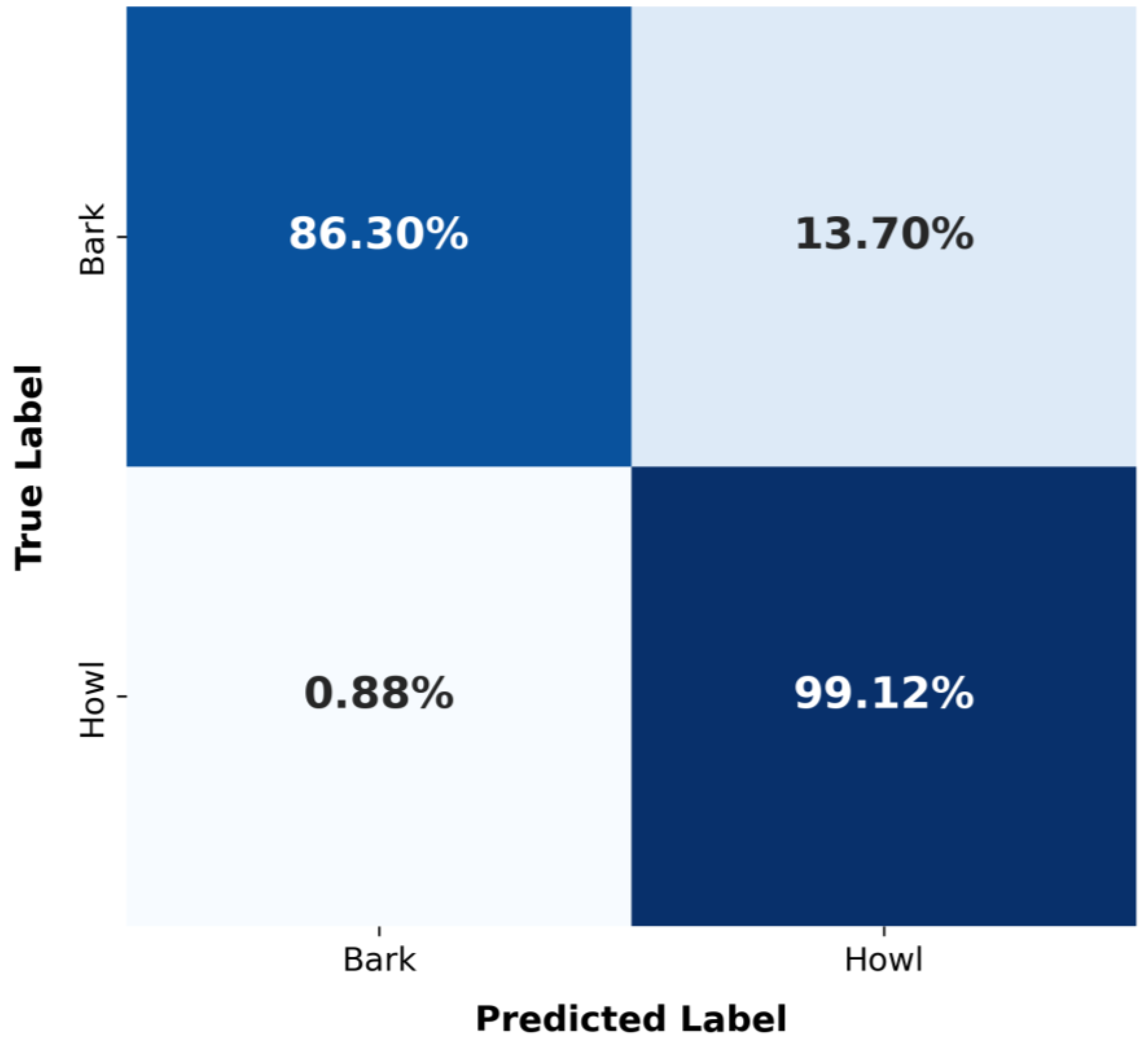
The row-normalized confusion matrix in Figure 3 shows that 86.30% of Bark decisions and 99.12% of Howl decisions were correct across the repeated evaluation. Bark-to-Howl errors were more frequent than Howl-to-Bark errors. The percentages describe the aggregated class-level error pattern; run-to-run variability is reported separately in Table 3.

3.2. Controlled Additive-Noise Performance

Table 4. Performance under Gaussian additive noise across ten repetitions of five-fold cross-validation. Each cell reports mean ± SD and the 95% CI.

Condition	Accuracy (%)	Macro Precision (%)	Macro Sensitivity (%)	Macro F1 (%)
No added noise	93.40 ± 2.62 [91.52–95.27]	94.43 ± 2.22 [92.84–96.02]	92.71 ± 2.86 [90.67–94.76]	93.20 ± 2.75 [91.23–95.16]
30 dB	93.40 ± 2.62 [91.52–95.27]	94.43 ± 2.22 [92.84–96.02]	92.71 ± 2.86 [90.67–94.76]	93.20 ± 2.75 [91.23–95.16]
20 dB	93.59 ± 2.30 [91.95–95.24]	94.57 ± 1.99 [93.14–95.99]	92.93 ± 2.50 [91.14–94.72]	93.41 ± 2.40 [91.69–95.12]
15 dB *	94.08 ± 2.35 [92.39–95.76]	94.89 ± 2.17 [93.34–96.44]	93.50 ± 2.52 [91.69–95.30]	93.92 ± 2.44 [92.18–95.66]
10 dB	94.76 ± 2.11 [93.25–96.26]	95.28 ± 1.99 [93.85–96.71]	94.34 ± 2.24 [92.73–95.95]	94.64 ± 2.16 [93.10–96.19]
5 dB	94.56 ± 3.43 [92.11–97.02]	94.73 ± 3.32 [92.35–97.10]	94.63 ± 3.28 [92.28–96.97]	94.51 ± 3.43 [92.06–96.97]
0 dB	79.42 ± 6.95 [74.44–84.39]	83.30 ± 4.01 [80.43–86.16]	81.13 ± 6.36 [76.58–85.68]	79.06 ± 7.79 [73.49–84.64]

* The 15 dB SNR condition was excluded from training and used only during evaluation.

and

Table 5. Performance under uniform additive noise across ten repetitions of five-fold cross-validation. Each cell reports mean ± SD and the 95% CI.

Condition	Accuracy (%)	Macro Precision (%)	Macro Sensitivity (%)	Macro F1 (%)
30 dB	93.40 ± 2.62 [91.52–95.27]	94.43 ± 2.22 [92.84–96.02]	92.71 ± 2.86 [90.67–94.76]	93.20 ± 2.75 [91.23–95.16]
20 dB	93.59 ± 2.30 [91.95–95.24]	94.57 ± 1.99 [93.14–95.99]	92.93 ± 2.50 [91.14–94.72]	93.41 ± 2.40 [91.69–95.12]
15 dB *	94.08 ± 2.44 [92.33–95.82]	94.90 ± 2.22 [93.31–96.48]	93.50 ± 2.63 [91.62–95.37]	93.92 ± 2.53 [92.11–95.73]
10 dB	94.66 ± 2.34 [92.98–96.34]	95.15 ± 2.28 [93.52–96.79]	94.27 ± 2.45 [92.52–96.03]	94.55 ± 2.40 [92.84–96.26]
5 dB	94.56 ± 3.75 [91.88–97.25]	94.66 ± 3.66 [92.05–97.28]	94.63 ± 3.59 [92.06–97.19]	94.52 ± 3.76 [91.83–97.20]
0 dB	79.42 ± 7.28 [74.21–84.62]	83.50 ± 4.06 [80.60–86.41]	81.17 ± 6.65 [76.42–85.93]	79.02 ± 8.22 [73.14–84.90]

* The 15 dB SNR condition was excluded from training and used only during evaluation.

report the repeated results under Gaussian and uniform additive noise. Mean accuracy and macro F1-score remained within the observed run-to-run variation between 30 and 5 dB SNR. The 15 dB condition was not included in training, yet its results remained comparable to adjacent SNR levels. At 0 dB, where signal and noise powers were equal, performance declined substantially for both noise distributions.

The numerical increases observed at several intermediate SNR levels should not be interpreted as evidence that noise improves classification. Their confidence intervals overlap the no-added-noise interval. The appropriate interpretation is that performance remained stable within repeated-run variability from 30 to 5 dB and degraded clearly at 0 dB.

3.3. Seed-42 Ablation Results

Table 6. Seed-42 reference ablation results. Values are pooled five-fold accuracies for the indicated test condition.

Configuration	No-Added-Noise Accuracy (%)	Gaussian 5 dB (%)	Uniform 5 dB (%)
Full model, 2 s	93.20	89.32	88.35
Without noise augmentation	94.17	68.93	68.93
Without batch normalization	90.29	88.35	87.38
Without dropout	91.26	87.38	86.41
1 s input duration	82.52	81.55	84.47
3 s input duration	92.23	89.32	89.32

reports the ablation experiments conducted with the seed-42 reference partitioning procedure. Removing noise augmentation increased no-added-noise accuracy from 93.20% to 94.17%, but reduced accuracy at 5 dB to 68.93% for both Gaussian and uniform noise. Removing batch normalization or dropout also reduced no-added-noise performance. A 1.0 s input caused the largest no-added-noise loss, whereas a 3.0 s input provided no consistent advantage over the 2.0 s reference configuration.

The seed-42 reference ablation provides descriptive support for the selected training design. The no-added-noise increase without augmentation was less than one percentage point, whereas the 5 dB loss was approximately 20 percentage points. In this reference run, batch normalization and dropout supported no-added-noise performance, and the duration experiment favored 2.0 s as a practical compromise between temporal context and acquisition cost. Because these ablations were not repeated across seeds, small differences should not be interpreted as statistical estimates.

3.4. Computational Results

The proposed model contains 7130 trainable parameters. With 32-bit floating-point storage, its model size is 27.85 KB. Using Equations (14)–(16), the model requires 18.35 MFLOPs for one 2.0 s segment. CPU and GPU inference times were 0.62 ms and 0.37 ms per segment, respectively. These values exclude the audio acquisition window.

Table 7. Computational profile of the proposed 1D-CNN.

Parameters	Model Size (KB)	Conv1D FLOPs	FC FLOPs	Total FLOPs	CPU (ms/Sample)	GPU (ms/Sample)
7130	27.85	18.35 M	0.001 M	18.35 M	0.62	0.37

summarizes the computational profile of the proposed 1D-CNN.

3.5. Contextual Comparison with Published Architectures

Table 8. Contextual comparison with selected feature-based CNN configurations reported by Karaaslan et al. [1].

Model	Input	Protocol	ACC (%)	SEN (%)	PRE (%)	F1 (%)	Params	FLOPS
AlexNet	MFCC	80/20 split	90.00	90.00	90.00	90.00	61.1 M	714 M
DenseNet	Mel spectrogram	80/20 split	90.00	90.00	90.00	90.00	8.0 M	2.9 G
EfficientNet	LFCC	80/20 split	90.00	90.00	90.00	90.00	5.3 M	390 M
ResNet50	MFCC/LFCC	80/20 split	86.00	86.00	85.00	86.00	25.6 M	4.1 G
ResNet152	MFCC/LFCC	80/20 split	86.00	86.00	85.00	86.00	60.2 M	11.3 G
Proposed	Raw waveform	10 × five-fold CV	93.40 ± 2.62	92.71 ± 2.86	94.43 ± 2.22	93.20 ± 2.75	7.13 K	18.35 M

places the repeated no-added-noise result alongside selected configurations reported by Karaaslan et al. [1] for the same source Bark and Howl dataset. The table is intended to provide task-specific context. It is not a strict benchmark, because the input representations, model configurations, training procedures, and evaluation protocols were not identical.

The operation values for the reference image CNNs are included only for contextualization. Input sizes and counting conventions may differ from the explicit FLOPs convention used for the proposed model.

Table 9. Contextual computational comparison with representative compact audio architectures. Values are those reported in the cited studies and are not directly comparable across tasks or counting conventions.

Architecture	Input	Task	Parameters	Reported Operation Count
BC-ResNet-1 [16]	Log-Mel spectrogram	Keyword spotting	9.2 K	3.1 M multiplications
Micro-ACDNet [18]	Raw waveform	Environmental sound classification	131 K	14.82 M FLOPs
Proposed model	Raw waveform	Bark/Howl classification	7.13 K	18.35 M FLOPs

provides a complementary efficiency context using representative compact audio architectures. BC-ResNet-1 processes log-Mel features for keyword spotting, whereas Micro-ACDNet processes raw waveforms for environmental sound classification [16,18]. The models were evaluated on different tasks, datasets, input durations, and operation-counting conventions. Their reported accuracies are therefore not compared with the Bark and Howl results.

4. Discussion

4.1. Classification Performance and Statistical Stability

The repeated evaluation provides a more informative estimate than a single five-fold run. Mean no-added-noise accuracy was 93.40 ± 2.62%, and mean macro F1-score was 93.20 ± 2.75%. The corresponding confidence intervals indicate moderate run-to-run variability, which is expected for a dataset of 103 recordings. The seed-42 result reported in the initial submission falls within these intervals and should be interpreted as one reference realization rather than the sole performance estimate.

The aggregate confusion matrix reveals a persistent class asymmetry. Howl sensitivity was higher than Bark sensitivity, whereas Bark predictions were highly precise. This pattern suggests that several Bark recordings contain temporal characteristics that resemble sustained Howl patterns. Because individual dog identities are unknown, part of the observed separation may also reflect subject-specific acoustic cues. The current results therefore represent recording-level classification performance.

4.2. Controlled Additive Noise and Ablation Findings

Repeated results remained stable within observed variability from 30 to 5 dB for both Gaussian and uniform additive noise. The unseen 15 dB condition also remained within the same range. This supports stability across the evaluated SNR grid, but only for the two analytically defined additive distributions. At 0 dB, mean accuracy decreased by approximately 14 percentage points relative to the no-added-noise mean, indicating that the model is vulnerable when noise power equals signal power.

The seed-42 ablation provides descriptive evidence about the training design. Removing noise augmentation preserved no-added-noise performance but caused a large decline at 5 dB, indicating that augmentation substantially supported resistance to controlled corruption in the reference run. Removing batch normalization or dropout reduced no-added-noise accuracy. The 1 s input omitted useful temporal context, whereas extending the window to 3 s did not provide a consistent advantage and increased the acquisition period. The 2 s configuration therefore offers a reasonable task-specific compromise. Because the ablations were not repeated across seeds, these differences should be interpreted descriptively rather than as statistical estimates.

The current noise experiments do not establish robustness to human speech, traffic, wind, rain, other animal sounds, reverberation, overlapping sources, microphone response, or recording distance. Adding a limited collection of environmental clips to the original recordings would still constitute simulated mixing and would depend strongly on source selection, room characteristics, and temporal alignment. Rigorous field robustness requires an independently designed external study with source-disjoint environmental recordings, multiple devices, and independently collected dog vocalizations.

4.3. Computational Efficiency and Relation to Compact Audio Models

The proposed model uses 7130 parameters and 27.85 KB of 32-bit storage. Its measured inference time was below 1 ms after segment acquisition. These properties are relevant to edge-oriented audio processing. The comparison with BC-ResNet-1 and Micro-ACDNet shows that compact audio models can be designed with parameter counts ranging from fewer than 10,000 to approximately 131,000 [16,18]. The proposed model therefore has a comparatively small parameter count. Its direct processing of 32,000 waveform samples, however, does not yield the lowest reported operation count among compact audio systems.

Inference time should not be conflated with end-to-end decision latency. The current system requires a 2.0 s waveform before classification. A deployed streaming system could use overlapping windows, but this would alter both latency and computational demand. Hardware-specific profiling on embedded devices is required before deployment suitability can be established.

4.4. Interpretation of Literature Comparisons

The feature-based comparison in Table 8 places the result in the context of the source dataset, but it is not a head-to-head benchmark. The reference CNNs used different representations, training configurations, and an 80/20 split, whereas the proposed result is the mean of ten repeated five-fold procedures. Accordingly, the numerical difference in accuracy cannot be attributed solely to the architecture or raw-waveform input. The comparison supports feasibility and computational compactness, not statistical superiority over the published systems. Thus, the comparison should be interpreted as task-specific context rather than as evidence of controlled superiority.

Likewise, the compact audio models in Table 9 were developed for keyword spotting or environmental sound classification using substantially larger datasets and different input representations. Their parameter and operation counts provide design context only. These comparisons are provided for contextual interpretation and should not be regarded as controlled head-to-head benchmarks, because the studies differ in feature representation, model setting, input duration, dataset, and evaluation protocol. A definitive accuracy-efficiency comparison would require faithful reimplementation, architecture-specific input adaptation, identical recording partitions, and equivalent hyperparameter-tuning budgets. Such a benchmark was not undertaken because it constitutes a separate controlled study and could be strongly influenced by implementation and tuning choices on only 103 recordings. The revised manuscript therefore avoids superiority claims and identifies same-protocol benchmarking as future work.

4.5. Limitations and Future Work

The principal limitation is the dataset size. Only 103 labeled recordings are available, which restricts coverage of breeds, ages, recording devices, acoustic environments, and behavioral contexts. Although repeated cross-validation improves the characterization of partition and training variability, it cannot remove the biological and acoustic limitations caused by the small public dataset or substitute for independent external validation.

A second limitation is the absence of individual dog identifiers. The number of unique subjects cannot be determined, and recordings from the same dog may occur in training and test folds. The model may therefore have exploited individual specific acoustic signatures in addition to vocalization-type characteristics. Subject-disjoint or Leave-One-Subject-Out evaluation remains necessary before generalization to unseen dogs can be claimed.

Third, the task includes only Bark and Howl. The model does not classify growling, whining, yelping, or non-dog acoustic events. Fourth, fixed-length standardization may discard late information in long recordings and introduce silent padding in short recordings. Fifth, the controlled-noise analysis is restricted to Gaussian and uniform additive corruption. Real environmental interference, reverberation, overlapping sources, microphone variability, and field recordings were not evaluated. Sixth, no separate validation subset was used; the epoch count and hyperparameters were fixed before the final analysis, and the held-out folds were reserved for final testing. Seventh, the ablation study used one seed-42 reference procedure and should be interpreted as diagnostic rather than as a complete repeated statistical comparison. Finally, no lightweight baseline was reimplemented under an identical training and tuning protocol, so the literature comparisons remain contextual.

Future work should use larger datasets with explicit subject identifiers, independent external test recordings, additional vocalization and rejection classes, and subject-disjoint evaluation. It should also examine realistic field recordings, room impulse responses, multiple devices, sliding-window inference, embedded hardware, and interpretation of learned temporal filters.

5. Conclusions

This study evaluated a compact 1D-CNN for Bark and Howl classification directly from 2.0 s raw audio waveforms under no-added-noise and controlled additive-noise conditions. The network contains 7130 trainable parameters, occupies 27.85 KB with 32-bit weights, and requires 18.35 MFLOPs.

Across ten repetitions of five-fold cross-validation, mean no-added-noise accuracy was 93.40 ± 2.62%, and mean macro F1-score was 93.20 ± 2.75%. Performance remained within run-to-run variability from 30 to 5 dB SNR for Gaussian and uniform additive noise, whereas mean accuracy decreased to 79.42% at 0 dB. In the seed-42 reference ablation, noise augmentation substantially preserved 5 dB accuracy, while batch normalization, dropout, and the 2 s input duration supported the selected configuration. These ablation findings are descriptive and are not repeated statistical estimates.

These results provide preliminary recording-level evidence that a small raw-waveform CNN can support efficient binary dog vocalization classification under controlled conditions. Because the dataset contains only 103 recordings, the findings should not be interpreted as evidence of broad practical generalization. Validation on larger, more diverse, and subject-identified datasets is required before practical applicability can be claimed. The results also do not establish subject-independent generalization or robustness to real field environments. Validation on independent recordings, realistic environmental interference, and multiple recording devices is required before broader biological or deployment claims can be made.

References

1. Karaaslan, M.; Turkoglu, B.; Kaya, E.; Asuroglu, T. Voice analysis in dogs with deep learning: Development of a fully automatic voice analysis system for bioacoustics studies. Sensors 2024, 24, 7978. [Google Scholar] [CrossRef] [PubMed]
2. Ovaskainen, O.; de Camargo, U.M.; Somervuo, P. Animal Sound Identifier (ASI): Software for automated identification of vocal animals. Ecol. Lett. 2018, 21, 1244–1254. [Google Scholar] [CrossRef] [PubMed]
3. Penar, W.; Magiera, A.; Klocek, C. Applications of bioacoustics in animal ecology. Ecol. Complex. 2020, 43, 100847. [Google Scholar] [CrossRef]
4. Siegford, J.M.; Steibel, J.P.; Han, J.; Benjamin, M.; Brown-Brandl, T.; Dórea, J.R.; Morris, D.; Norton, T.; Psota, E.; Rosa, G.J. The quest to develop automated systems for monitoring animal behavior. Appl. Anim. Behav. Sci. 2023, 265, 106000. [Google Scholar] [CrossRef]
5. Teixeira, D.; Maron, M.; van Rensburg, B.J. Bioacoustic monitoring of animal vocal behavior for conservation. Conserv. Sci. Pract. 2019, 1, e72. [Google Scholar] [CrossRef]
6. Taylor, A.M.; Reby, D.; McComb, K. Context-related variation in the vocal growling behaviour of the domestic dog (Canis familiaris). Ethology 2009, 115, 905–915. [Google Scholar] [CrossRef]
7. Yin, S.; McCowan, B. Barking in domestic dogs: Context specificity and individual identification. Anim. Behav. 2004, 68, 343–355. [Google Scholar] [CrossRef]
8. Yeo, C.Y.; Al-Haddad, S.; Ng, C.K. Dog voice identification (ID) for detection system. In 2012 Second International Conference on Digital Information Processing and Communications (ICDIPC); IEEE: New York, NY, USA, 2012. [Google Scholar] [CrossRef]
9. Bishop, J.C.; Falzon, G.; Trotter, M.; Kwan, P.; Meek, P.D. Livestock vocalisation classification in farm soundscapes. Comput. Electron. Agric. 2019, 162, 531–542. [Google Scholar] [CrossRef]
10. Nunes, L.; Ampatzidis, Y.; Costa, L.; Wallau, M. Horse foraging behavior detection using sound recognition techniques and artificial intelligence. Comput. Electron. Agric. 2021, 183, 106080. [Google Scholar] [CrossRef]
11. Tsai, M.-F.; Huang, J.-Y. Sentiment analysis of pets using deep learning technologies in artificial intelligence of things system. Soft Comput. 2021, 25, 13741–13752. [Google Scholar] [CrossRef]
12. Palanisamy, K.; Singhania, D.; Yao, A. Rethinking CNN models for audio classification. arXiv 2020, arXiv:2007.11154. [Google Scholar] [CrossRef]
13. Abdoli, S.; Cardinal, P.; Koerich, A.L. End-to-end environmental sound classification using a 1D convolutional neural network. Expert Syst. Appl. 2019, 136, 252–263. [Google Scholar] [CrossRef]
14. Dai, W.; Dai, C.; Qu, S.; Li, J.; Das, S. Very deep convolutional neural networks for raw waveforms. In 2017 IEEE International Conference on Acoustics, Speech and Signal Processing (ICASSP); IEEE: New York, NY, USA, 2017. [Google Scholar] [CrossRef]
15. Choi, S.; Seo, S.; Shin, B.; Byun, H.; Kersner, M.; Kim, B.; Kim, D.; Ha, S. Temporal convolution for real-time keyword spotting on mobile devices. arXiv 2019, arXiv:1904.03814. [Google Scholar] [CrossRef]
16. Kim, B.; Chang, S.; Lee, J.; Sung, D. Broadcasted residual learning for efficient keyword spotting. arXiv 2021, arXiv:2106.04140. [Google Scholar] [CrossRef]
17. Majumdar, S.; Ginsburg, B. Matchboxnet: 1d time-channel separable convolutional neural network architecture for speech commands recognition. arXiv 2020, arXiv:2004.08531. [Google Scholar] [CrossRef]
18. Mohaimenuzzaman, M.; Bergmeir, C.; West, I.; Meyer, B. Environmental Sound Classification on the Edge: A Pipeline for Deep Acoustic Networks on Extremely Resource-Constrained Devices. Pattern Recognit. 2023, 133, 109025. [Google Scholar] [CrossRef]
19. Nanni, L.; Maguolo, G.; Paci, M. Data augmentation approaches for improving animal audio classification. Ecol. Inform. 2020, 57, 101084. [Google Scholar] [CrossRef]
20. Salamon, J.; Bello, J.P. Deep convolutional neural networks and data augmentation for environmental sound classification. IEEE Signal Process. Lett. 2017, 24, 279–283. [Google Scholar] [CrossRef]
21. Loizou, P.C. Speech Enhancement: Theory and Practice; CRC Press: Boca Raton, FL, USA, 2007. [Google Scholar] [CrossRef]
22. LeCun, Y.; Bottou, L.; Bengio, Y.; Haffner, P. Gradient-based learning applied to document recognition. Proc. IEEE 1998, 86, 2278–2324. [Google Scholar] [CrossRef]
23. Ioffe, S.; Szegedy, C. Batch normalization: Accelerating deep network training by reducing internal covariate shift. In Proceedings of the International Conference on Machine Learning, Lille, France, 6–11 July 2015. Proceedings of Machine Learning Research (PMLR). [Google Scholar]
24. Glorot, X.; Bordes, A.; Bengio, Y. Deep sparse rectifier neural networks. In Proceedings of the Fourteenth International Conference on Artificial Intelligence and Statistics; JMLR Workshop and Conference Proceedings; JMLR.org: Norfolk, MA, USA, 2011. [Google Scholar]
25. Nair, V.; Hinton, G.E. Rectified linear units improve restricted boltzmann machines. In Proceedings of the 27th International Conference on Machine Learning (ICML-10), Haifa, Israel, 21–24 June 2010. [Google Scholar]
26. Lin, M.; Chen, Q.; Yan, S. Network in network. arXiv 2013, arXiv:1312.4400. [Google Scholar] [CrossRef]
27. Srivastava, N.; Hinton, G.; Krizhevsky, A.; Sutskever, I.; Salakhutdinov, R. Dropout: A simple way to prevent neural networks from overfitting. J. Mach. Learn. Res. 2014, 15, 1929–1958. [Google Scholar]
28. Dumoulin, V.; Visin, F. A guide to convolution arithmetic for deep learning. arXiv 2016, arXiv:1603.07285. [Google Scholar] [CrossRef]
29. Paszke, A.; Gross, S.; Massa, F.; Lerer, A.; Bradbury, J.; Chanan, G.; Killeen, T.; Lin, Z.; Gimelshein, N.; Antiga, L.; et al. Pytorch: An imperative style, high-performance deep learning library. In Advances in Neural Information Processing Systems; Curran Associates, Inc.: Red Hook, NY, USA, 2019; Volume 32. [Google Scholar]
30. Kinga, D.; Adam, J.B. A method for stochastic optimization. In Proceedings of the International Conference on Learning Representations (ICLR), San Diego, CA, USA, 7–9 May 2015. [Google Scholar]
31. Kohavi, R. A study of cross-validation and bootstrap for accuracy estimation and model selection. In Proceedings of the IJCAI, Montreal, QC, Canada, 20–25 August 1995. [Google Scholar]
32. Bengio, Y.; Grandvalet, Y. No unbiased estimator of the variance of k-fold cross-validation. J. Mach. Learn. Res. 2004, 5, 1089–1105. [Google Scholar]
33. Sokolova, M.; Lapalme, G. A systematic analysis of performance measures for classification tasks. Inf. Process. Manag. 2009, 45, 427–437. [Google Scholar] [CrossRef]
34. Sze, V.; Chen, Y.-H.; Yang, T.-J.; Emer, J.S. Efficient processing of deep neural networks: A tutorial and survey. Proc. IEEE 2017, 105, 2295–2329. [Google Scholar] [CrossRef]
Figure 1. Fixed-length raw waveform standardization for representative Bark and Howl samples. Dark segments indicate the 2.0 s region used by the model. Light segments indicate discarded portions, and dashed gray segments indicate zero padding.
Applsci 16 06819 g001
Figure 2. Overall architecture of the proposed 1D-CNN for Bark and Howl classification from raw audio waveforms.
Applsci 16 06819 g002
Figure 3. Row-normalized confusion matrix for the no-added-noise condition across ten repetitions of five-fold cross-validation. Cell values show percentages within each true class; raw counts are omitted because the same recordings were evaluated once per repetition.
Applsci 16 06819 g003