Liver Disease Prediction Using Hybrid Feature Selection: A Comparative Analysis of Machine Learning Models

Abstract

Liver disease represents a major global health burden, and early diagnosis is essential for reducing mortality. Machine learning (ML) approaches offer non-invasive alternatives to conventional diagnostics, yet existing studies on liver disease prediction often lack systematic feature selection, apply resampling before data splitting (introducing leakage), and report results from single train-test splits without statistical testing. This study proposes a Hybrid Feature Selection (HFS) framework combining Pearson-correlation-based redundancy elimination with a weighted Information Gain–Gain Ratio scoring function, integrated with SMOTE within a leakage-free pipeline. The framework is evaluated on two benchmarks—the Indian Liver Patient Dataset (ILPD, n = 583) and the BUPA Liver Disorders Dataset (n = 345)—across ten classifiers and ten independent train-test splits, with significance assessed via paired Wilcoxon signed-rank tests. On ILPD, the HFS + SMOTE pipeline produced statistically significant ROC-AUC improvements (p < 0.05) in five of ten classifiers and resolved majority-class collapse, raising mean Specificity from 0.00–0.33 to 0.61–0.92. A 2 × 2 ablation study confirmed that HFS and SMOTE contribute independently, with SMOTE driving the Specificity transformation and HFS reducing feature-space noise. Sensitivity analyses demonstrated robustness to the weighting parameter w and confirmed k = 6 as the optimal feature count. Replication on BUPA—which exhibits near-perfect class balance and no feature redundancy—produced a principled null result, confirming that the pipeline’s effectiveness is mechanistically linked to dataset characteristics. The HFS algorithm consistently identified four clinically meaningful core features (AST, ALT, Total Bilirubin, Age) across all runs, validated by SHAP and Permutation Importance stability analysis.

1. Introduction

Liver diseases represent a major global health burden encompassing a broad spectrum of conditions, including non-alcoholic fatty liver disease (NAFLD), metabolic dysfunction-associated steatotic liver disease (MASLD), viral hepatitis, cirrhosis, and hepatocellular carcinoma. These disorders account for millions of deaths annually and impose substantial economic and social costs on healthcare systems worldwide. Early and accurate diagnosis is critical not only for improving patient outcomes but also for reducing disease-related complications and mortality. However, conventional diagnostic approaches—largely dependent on invasive procedures such as liver biopsy, or expensive imaging modalities—remain inaccessible and impractical for large-scale screening. This reality has intensified the demand for non-invasive, cost-effective, and scalable diagnostic tools that can be deployed at the population level. Since early diagnosis and risk prediction play a critical role in preventing disease progression, machine learning-based approaches have received significant attention in this field in recent years. The application of machine learning (ML) to liver disease prediction has grown substantially over the past decade, producing a rich body of literature spanning classical statistical models, ensemble learning frameworks, deep learning architectures, explainability techniques, and feature selection strategies. A comprehensive review of recent advances in ML-based liver disease prediction is provided in Section 2.

The present study addresses these gaps by proposing a Hybrid Feature Selection (HFS) framework that sequentially applies Pearson correlation-based redundancy elimination and a weighted Information Gain–Gain Ratio scoring function to identify the six most informative clinical features. Ten classifiers—Logistic Regression, Decision Tree, KNN, Support Vector Machine with RBF kernel, Support Vector Machine with Linear kernel, Random Forest, AdaBoost, Bagging, XGBoost, and a Stacking ensemble combining Random Forest and SVM-RBF base learners with a Logistic Regression meta-learner—are then trained and evaluated under identical experimental conditions, with statistical significance assessed across ten independent train-test splits, enabling a rigorous and reproducible comparative analysis of algorithmic performance before and after feature selection on the ILPD benchmark.

2. Related Work

Early efforts in liver disease prediction relied predominantly on classical supervised learning algorithms applied to structured clinical and biochemical datasets. Logistic Regression (LR), Support Vector Machine (SVM), K-Nearest Neighbor (KNN), Decision Tree (DT), and Naive Bayes classifiers have been widely used as baseline models owing to their computational efficiency and interpretability. Studies conducted on the Indian Liver Patient Dataset (ILPD)—a benchmark comprising 583 patient records with ten clinical attributes—consistently demonstrated that LR and SVM achieve stable predictive performance across different experimental configurations [1,2,3,4,5,6,7,8]. Modhugu and Ponnusamy conducted a large-scale comparative study on 21,000 Kaggle records, reporting that SVM yielded the highest accuracy (85%) among LR, SVM, and DT, while LR and DT reached 82% and 79%, respectively [9]. Similarly, Zhang confirmed that SVM with a Gaussian kernel outperformed RF on the same 583-patient Indian dataset in terms of non-invasive diagnostic accuracy [5]. İlter and Kırelli further demonstrated that LR achieved 80% accuracy on ILPD when paired with normalization and feature selection, while AdaBoost and RF also yielded competitive results [7]. Despite their interpretability, classical methods are consistently reported to struggle with complex non-linear feature interactions, noisy clinical measurements, and the class imbalance inherent in disease datasets [10,11].

Ensemble learning approaches have emerged as the dominant paradigm in liver disease classification, consistently surpassing classical methods across a range of performance metrics [12]. Random Forest (RF), Gradient Boosting (GB), AdaBoost, XGBoost, LightGBM, and CatBoost have all been investigated, with tree-based boosting algorithms proving particularly effective. Wu et al. applied RF, Naive Bayes, Artificial Neural Networks, and LR to a cohort of 577 patients in Taiwan, finding that RF achieved the highest AUROC (0.925) and accuracy (87.48%) in 10-fold cross-validation, substantially outperforming competing methods [13]. Quadir et al. evaluated GB, XGBoost, Bagging, RF, Extra Trees, and Stacking on ILPD with advanced preprocessing; Extra Trees reached 91.82% and RF 86.06% test accuracy, exceeding prior literature benchmarks [14]. Mohamed et al. proposed a two-level ensemble stacking model on ILPD that, combined with feature selection, achieved 94.01% accuracy, 94.44% precision, and a 94.25% AUC in 10-fold cross-validation [15]. Ganie and Pramanik provided the most exhaustive boosting comparison to date, testing seven algorithms—GB, AdaBoost, LogitBoost, SGBoost, XGBoost, LightGBM, and CatBoost—on both ILPD and LDPD with hyperparameter tuning; GB emerged as the best performer, with 98.80% and 98.29% accuracy on the respective datasets across twelve evaluation metrics [16].

El Atifi et al. showed that an optimized RF (GridSearchCV) attained 85.17% accuracy with balanced precision and recall, outperforming AdaBoost and GB variants [17]. Rani et al. combined SMOTE-ENN oversampling with RFE-based feature selection, constructing SMOTEENN-KNN and SMOTEENN-AdaBoost hybrid models that reached 93.2% accuracy on ILPD and 95.4% on BUPA, with very low Brier Score losses (0.031–0.032) [11]. Jasim et al. and Gupta et al. further confirmed that ensemble methods—particularly XGBoost—provide superior generalization on diverse liver datasets [1,18]. Qin et al. systematically evaluated multiple ML classifiers for screening NAFLD in a general adult population, demonstrating that ensemble-based approaches consistently outperformed single-algorithm baselines in terms of AUC and calibration [19]. Similarly, Razmpour et al. applied a battery of ML algorithms, including RF, XGBoost, and SVM to predict NAFLD using anthropometric and body composition indices, confirming that ensemble methods leveraging accessible physical measurements can achieve clinically adequate predictive performance without the need for laboratory tests [20]. Collectively, these findings establish boosting-based ensembles as the current state of the art for tabular clinical data.

Deep learning methods have attracted increasing interest in hepatology due to their capacity to extract hierarchical representations from high-dimensional data without manual feature engineering. Lanjewar et al. proposed a cloud-integrated framework that combined CNN-based feature extraction with LR, SVM, and RF classifiers, employing ExtraTreesClassifier and Maximum Relevance Minimum Redundancy (MRMR) for feature selection; the CNN-RF combination achieved 100% precision under stratified K-fold cross-validation [21]. Hendi et al. introduced a hybrid CNN + LSTM architecture that modeled both spatial and temporal dependencies in complex hepatic data, attaining 98.73% accuracy, 99% precision, and 99% AUC—the highest reported accuracy in the surveyed literature [22]. Standard LSTM, RNN, and CNN baselines were all outperformed. Chen et al. proposed a Dual Graph Attention Network (DGAN) that framed NAFLD diagnosis in patients with Type 2 Diabetes as a node classification task on a graph, leveraging both feature similarity and patient topology from 2402 patient records [23]. This architecture demonstrated superior accuracy over conventional models, illustrating the potential of graph-based deep learning for structured patient data. Donaire et al. explored a hybrid quantum-classical approach (QML-Liver) on ILPD, showing that quantum machine learning can deliver competitive F1-scores while reducing qubit requirements to two, opening a promising direction for resource-efficient diagnostics [24]. Despite these advances, deep learning models require substantially larger training sets than are typically available in single-center clinical studies, and their internal representations remain opaque without additional interpretability mechanisms. This limitation has stimulated widespread adoption of explainable AI methods, reviewed in the following subsection.

The integration of Explainable AI (XAI) techniques has become a central concern in ML-based liver disease research, as high predictive accuracy alone is insufficient for clinical adoption. SHAP (SHapley Additive exPlanations) and LIME (Local Interpretable Model-agnostic Explanations) are the two most widely used tools for rendering complex model decisions transparent at both global and local levels [25,26]. Khan et al. proposed an integrated XAI framework combining a Boosting Classifier (90.88% accuracy) with SHAP and LIME analyses on 1700 patient records, identifying liver function tests, alcohol consumption, and age as the most influential predictors [25]. Makkena and Natarajan applied an XGBoost-XAI model for non-invasive cirrhosis diagnosis, achieving 91.19% accuracy and demonstrating how XAI tools reveal clinically meaningful decision pathways that increase physician trust [26]. Yu et al. applied RFE-selected RF on 13,436 NHANES participants, attaining AUC values of 0.928 (internal) and 0.918 (external); SHAP analysis highlighted waist circumference, BMI, and metabolic biomarkers as the dominant MASLD predictors [27]. Hong et al. similarly used the Boruta algorithm for feature selection and SHAP for interpretation in a MAFLD study on NHANES data, finding that visceral adipose tissue (VAT) was the strongest determinant—a finding not recoverable from BMI alone [28]. Beyond diagnosis, SHAP analyses have been applied to cardiovascular risk stratification in MAFLD patients [29], HCC risk prediction in HBV-cACLD cohorts [30], diabetes risk in MASLD patients [31], and atrial fibrillation identification in NAFLD patients [32]. In each case, XAI revealed that standard clinical markers (ALT, AST, bilirubin, albumin, age) align with established hepatological knowledge, reinforcing model reliability while offering personalized risk profiles that purely numerical outputs cannot provide. Zhou et al. developed an interpretable ML model for predicting MASLD in patients with Type 2 Diabetes, employing SHAP-driven feature attribution to identify the most clinically relevant metabolic risk factors within this high-risk comorbid population [33]. Complementing this work, Gu and Chai constructed an interpretable ML pipeline for predicting significant liver fibrosis in patients with concurrent chronic hepatitis B and NAFLD, reporting that model interpretability substantially facilitated clinical validation and enhanced physician acceptance of the algorithmic output [34].

Feature selection and preprocessing have been consistently identified as critical determinants of model performance. Redundant or irrelevant features increase computational cost, reduce model generalizability, and can mask genuine clinical signals. A variety of filter, wrapper, and embedded selection methods have been applied in the liver disease prediction literature. LASSO regression has been employed for variable reduction in several large-cohort studies [30,31,35,36,37]. Boruta, a wrapper method based on RF permutation tests, was used by Hong et al. and Zhang et al. to identify robust feature subsets robust to noise [28,32]. Recursive Feature Elimination (RFE) was adopted by Rani et al., Yu et al., and Xu et al., each reporting meaningful accuracy gains after dimensionality reduction [11,27,38]. Ma et al. relied on a Bayesian network in which the five most discriminative features for NAFLD prediction—BMI, triglycerides, GGT, ALT, and uric acid—were selected through model-internal importance ranking, achieving 83% accuracy and a 9.17% F-measure improvement over LR [39].

Information-theoretic criteria such as Information Gain (IG) and Gain Ratio (GR) have received comparatively less attention in liver-specific studies, despite their effectiveness as filter-based metrics that quantify feature relevance with respect to the target class without incurring the computational overhead of wrapper methods. Pearson correlation-based redundancy elimination has been employed as a preprocessing step in several studies [3,14,15], but typically in isolation rather than as part of a unified hybrid scoring framework. Preprocessing strategies beyond feature selection have also been influential. Missing value imputation using mean or multivariate approaches, log-transformation of skewed biomarkers, StandardScaler normalization, and SMOTE or SMOTE-ENN-based class balancing have each been shown to produce substantial performance improvements on ILPD and related datasets [10,11,14,18,40]. Kuzhippallil et al. augmented XGBoost with a genetic algorithm for feature optimization, using Isolation Forest for outlier removal and reporting improvements in both accuracy and time complexity [41]. Khosravi et al. systematically compared four feature selection methods with eight classifiers on 3654 Iranian T2DM patients, finding that XGBoost without feature selection achieved the highest AUC (0.889), underscoring the importance of evaluating selection methods empirically rather than assuming universal benefit [40].

The clinical scope of ML-based liver disease research has expanded well beyond binary diagnosis to encompass risk stratification, comorbidity prediction, and population-level screening. Huang et al. developed a LASSO-RF pipeline on NHANES 2021–2023 to classify MAFLD risk into low, intermediate, and high categories, achieving AUC values of 0.80–0.83 across groups using 16 routinely accessible variables [35]. Xu et al. proposed a two-step “fibrosis-first” strategy using RF followed by MLP for NAS score assessment in a multicenter cohort of 840 biopsy-proven patients, demonstrating 84.7% accuracy and 87% specificity and substantially reducing dependence on invasive biopsy [38]. Several studies have targeted specific high-risk subpopulations. Li et al. built an RF model for HCC risk prediction in HBV-cACLD patients (AUC = 0.979), with SHAP identifying liver stiffness, platelets, and bile acids as the dominant predictors [30]. Wu et al. used LR as the most robust model for in-hospital mortality prediction in Acute Liver Failure (AUC = 0.802 internal, 0.774 external), validated on an independent cohort [36]. Rivera et al. applied ML classifiers to predict radioembolization-induced liver disease (REILD) after SIRT for HCC, defining a novel bilirubin threshold (26.5 μmol/L) for toxicity risk stratification [42]. Emerging interdisciplinary directions include metabolomic profiling [43], occupational exposure analysis [32], and quantum-classical hybrid diagnostics [24]. Dan et al. integrated untargeted metabolomics with ML on serum samples from 165 NAFLD patients, identifying maresin 1, paraxanthine, and 1-methyluric acid as novel diagnostic biomarkers with strong model-validated performance [43]. Lin et al. applied multiple ML classifiers to NHANES data for predicting MAFLD, incorporating the novel non-high-density lipoprotein cholesterol-to-high-density lipoprotein cholesterol ratio (NHHR) as an accessible composite metabolic marker and demonstrating its incremental value over conventional lipid indices [44]. He et al. integrated CT-derived body composition analysis with ML in a large-scale health examination cohort, showing that automated phenotyping of visceral fat, muscle mass, and liver attenuation substantially improves non-invasive MASLD identification beyond standard anthropometric indices [45]. Sadeghi et al. demonstrated that steatotic liver disease can be simultaneously diagnosed and graded using only routine clinical and laboratory variables, reporting that a well-calibrated ML pipeline achieved high concordance with imaging-based staging and substantially reduced the need for specialist referral [46]. Gao and Duan provided a comprehensive overview of the current status and future directions of AI in liver disease, situating prediction, diagnosis, and treatment planning within a unified translational framework and identifying data scarcity, model generalizability, and regulatory acceptance as the principal barriers to clinical deployment [47]. Yang et al. further synthesized recent advances in the application of ML models to MASLD, highlighting that multi-modal data integration, transfer learning, and federated approaches are emerging as the most promising strategies for overcoming the inherent limitations of single-center, single-modality studies [48]. Zhang et al. demonstrated that occupational heat exposure beyond 10 years, combined with petrochemical dust exposure, significantly elevates MAFLD risk (HR: 2.31–2.78) using XGBoost on a nested case-control cohort of 1277 workers [49]. These studies collectively expand the clinical utility of ML in hepatology toward personalized, preventive, and precision medicine applications.

Despite the substantial progress documented above, several critical methodological gaps persist in the liver disease prediction literature. First, the majority of studies employ all available features without systematic selection or adopt single-criterion filter methods (e.g., correlation alone, IG alone) that either ignore feature relevance or fail to account for redundancy between selected features. No prior work on ILPD-based liver disease prediction has proposed a hybrid filter framework that jointly addresses redundancy elimination and dual-criterion relevance scoring within a unified, computationally lightweight pipeline. Second, comparisons across ML classifiers are frequently conducted without controlling for the preprocessing configuration, making it difficult to attribute observed performance differences to algorithmic choice versus data preparation. Third, while ensemble methods dominate the literature, the relative behavior of diverse classifier families—from linear models to boosting to bagging—under identical hybrid feature selection conditions has not been systematically characterized on ILPD.

3. Materials and Methods

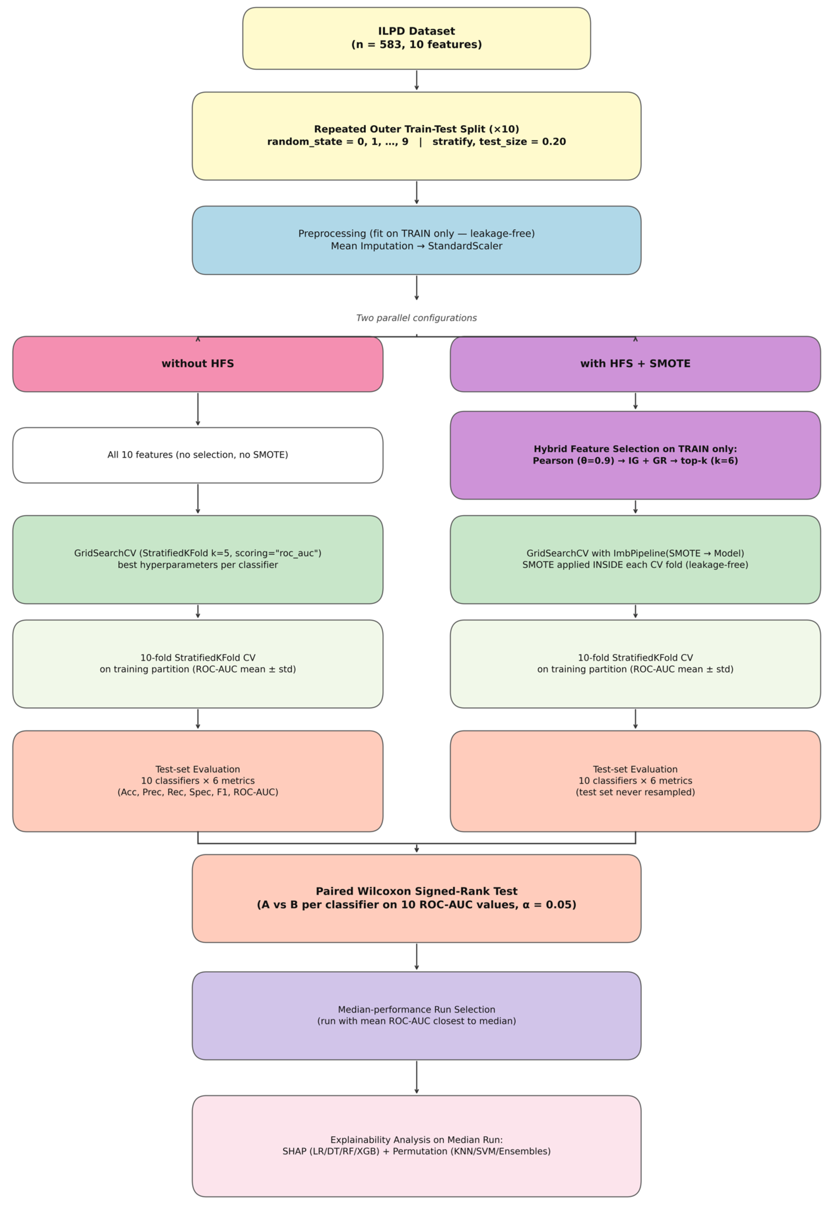
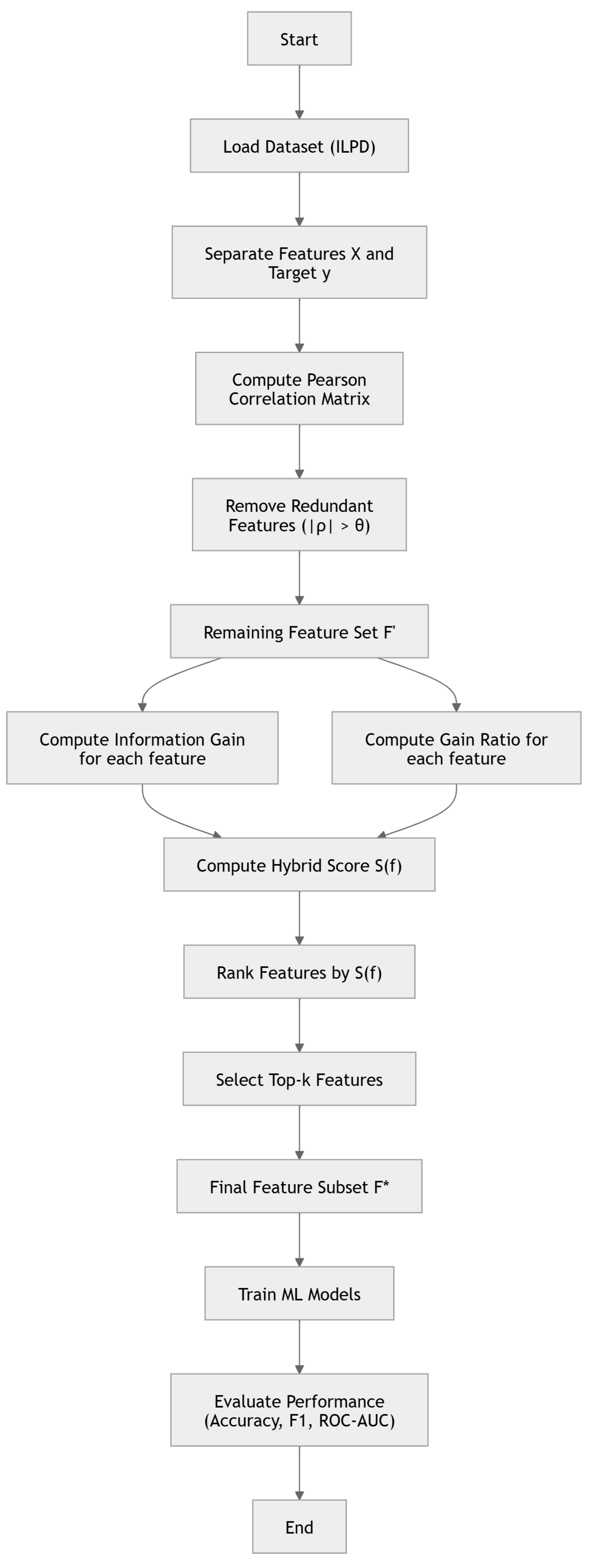
In this section, the methodology used to classify liver diseases is explained. The overall research framework is presented, starting with data preprocessing and preparation steps, followed by the feature selection process. In this context, a two-stage strategy is adopted to eliminate redundant information and identify the most discriminative features. Subsequently, multiple machine learning algorithms are trained using the selected features, and their performances are evaluated under consistent experimental settings. This approach enables a comprehensive assessment of both the impact of feature selection and the comparative effectiveness of different classifiers. The overall research framework is illustrated in Figure 1, while the detailed steps of the proposed Hybrid Feature Selection algorithm are shown in Figure 2. Two publicly available liver disease datasets—ILPD and BUPA—are used in this study to evaluate the proposed framework. The ILPD dataset serves as the primary benchmark, while BUPA provides a complementary generalizability assessment under different data characteristics.

3.1. ILPD Dataset and Preprocessing

The proposed approach is evaluated on the Indian Liver Patient Dataset (ILPD) [50], a widely used benchmark comprising 583 patient records, 10 clinical attributes, and a binary class label indicating liver disease presence. The dataset contains both numerical and categorical variables, including liver enzyme levels, bilirubin concentrations, protein ratios, patient age, and gender.

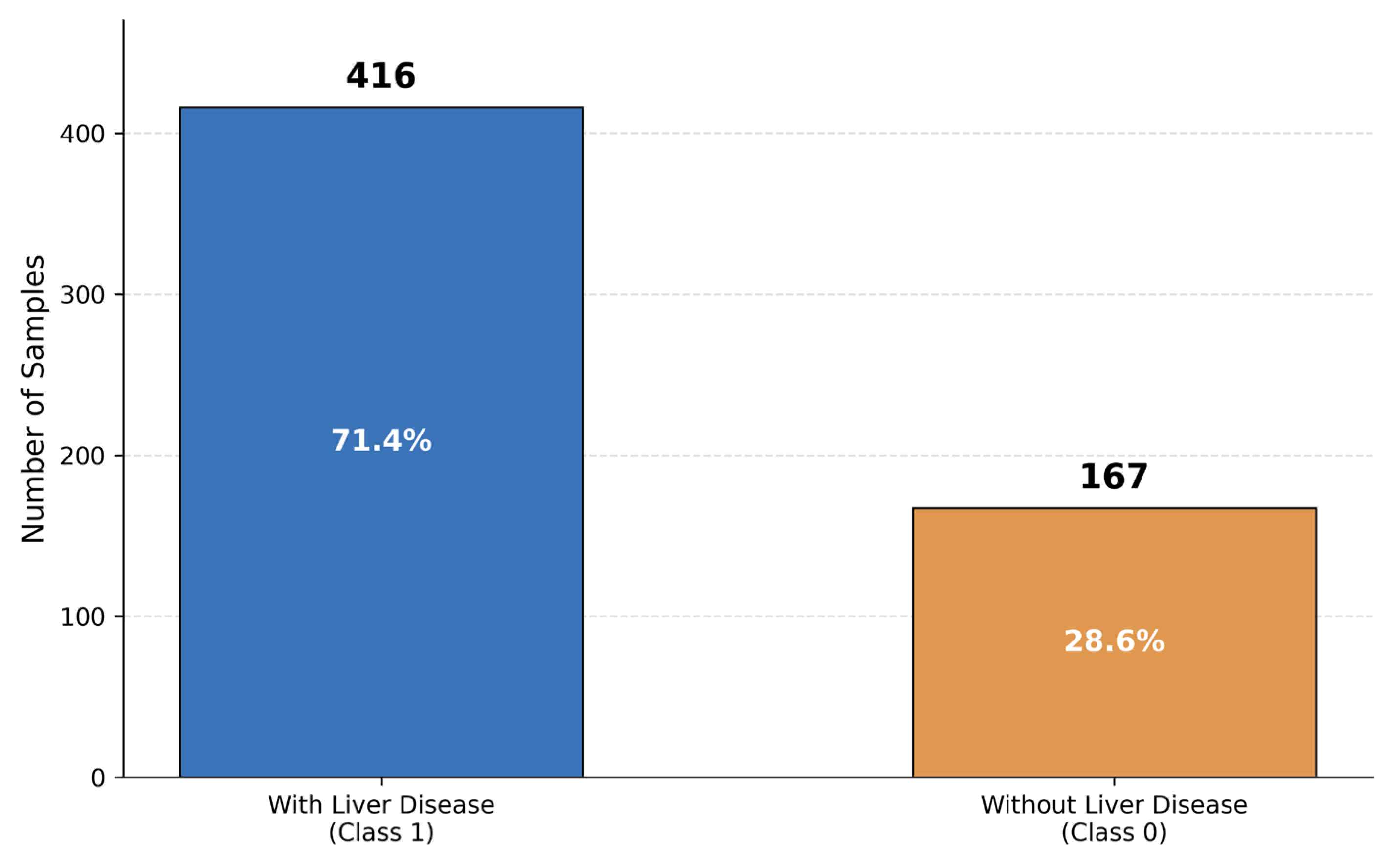
In the preprocessing stage, four operations were applied sequentially. First, missing values present in the Albumin-to-Globulin Ratio attribute were imputed using the feature mean. Second, the categorical gender attribute was encoded as a binary indicator (Male = 1, Female = 0). Third, the target variable was transformed into a standard binary format: the original label 2 (healthy) was mapped to 0, while label 1 (liver disease) was retained, yielding a class distribution of 416 positive (71.4%) and 167 negative (28.6%) instances, corresponding to an imbalance ratio (IR) of 2.49:1. Fourth, all numerical features were normalized using StandardScaler to produce zero-mean, unit-variance representations, thereby improving numerical stability and model convergence across classifiers with different optimization landscapes. The features are age, gender, total bilirubin (TB), direct bilirubin (DB), total proteins (TP), albumin (ALB), albumin and globulin ratio (A/G), alamine aminotransferase (SGPT), aspartate aminotransferase (SGOT), and alkaline phosphotase (Alkphos). The characteristics of all the features for the patients are tabulated in

Table 1. The characteristics of all the features for the patients.

Characteristics	Subgroup	All (Number)	All (%)	With Liver Disease (Number)	With Liver Disease (%)	Without Liver Disease (Number)	Without Liver Disease (%)
Patients Enrolled	-	583	100	416	71.36	167	28.65
Age (in years)	Median	45	-	46	-	40	-
	Range	4 to 90	-	7 to 90	-	4 to 85	-
Gender	Male	441	75.64	324	77.88	117	70.06
	Female	142	24.36	92	22.12	50	29.94
Total Bilirubin (TB)	Median	1	-	1.4	-	0.8	-
	Range	0.4 to 75	-	0.4 to 75	-	0.5 to 7.3	-
Direct Bilirubin (DB)	Median	0.3	-	0.5	-	0.2	-
	Range	0.1 to 19.7	-	0.1 to 19.7	-	0.1 to 3.6	-
Alkaline Phosphatase (AP)	Median	208	-	229	-	186	-
	Range	63 to 2110	-	63 to 2110	-	90 to 1590	-
Alanine Aminotransferase (SGPT)	Median	35	-	41	-	27	-
	Range	10 to 2000	-	12 to 2000	-	10 to 181	-
Aspartate Aminotransferase (SGOT)	Median	42	-	52.5	-	29	-
	Range	4 to 4929	-	11 to 4929	-	10 to 285	-
Total Proteins (TP)	Median	6.6	-	6.55	-	6.6	-
	Range	2.7 to 9.6	-	2.7 to 9.6	-	3.7 to 9.2	-
Albumin	Median	3.10	-	3.00	-	3.4	-
	Range	0.9 to 5.5	-	0.9 to 5.5	-	1.4 to 5.0	-
Albumin and Globulin Ratio	Median	0.93	-	0.90	-	1	-
	Range	0.3 to 2.8	-	0.3 to 2.8	-	0.37 to 1.9	-

. The output variable has two classes denoting patients with liver disease and those without. The dataset contains 583 records of patients collected from Andhra Pradesh’s North East region in India. The distribution of patients with and without liver disease is shown in Figure 3.

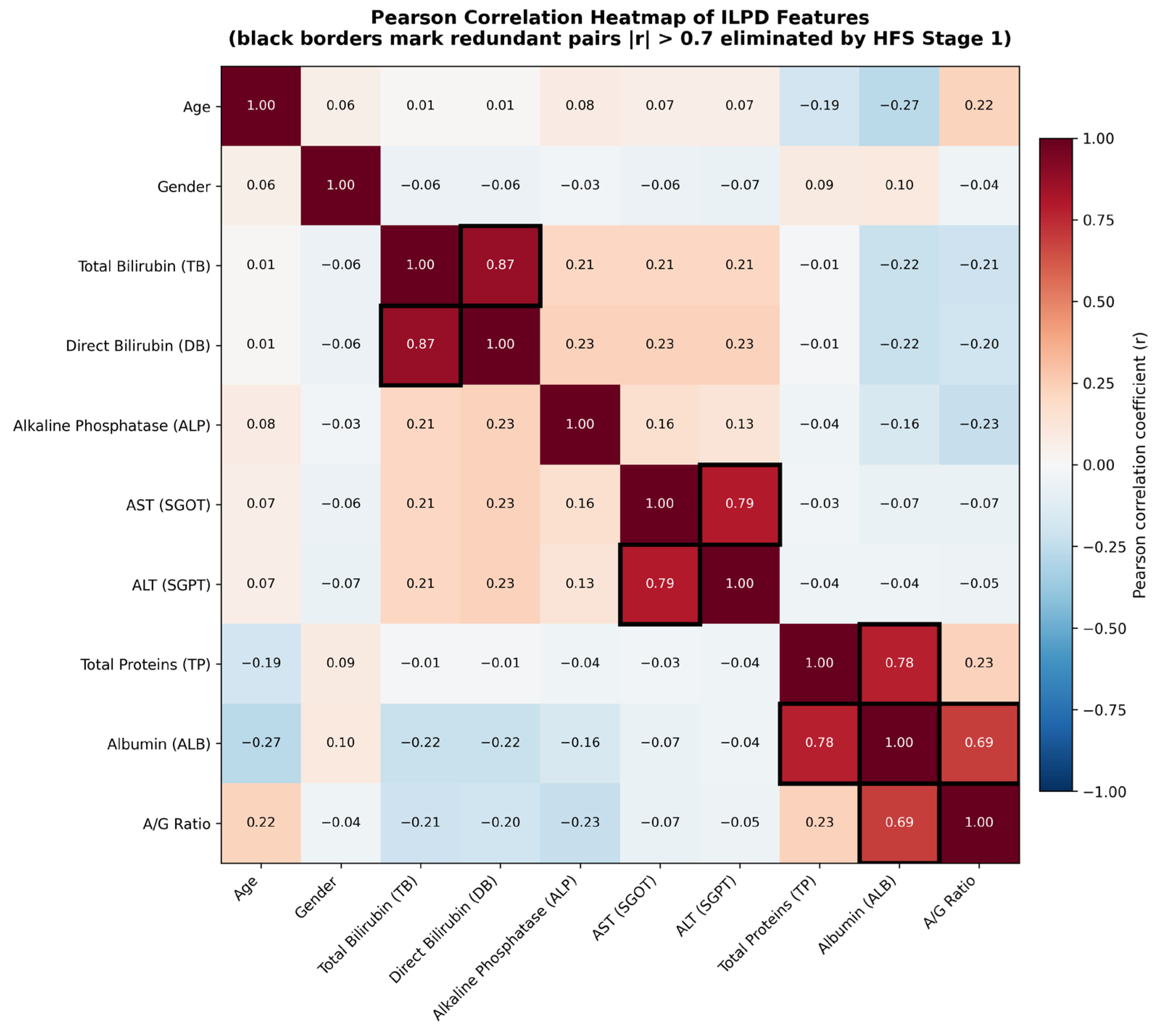
Beyond class imbalance, the ILPD also exhibits inter-feature correlation. A Pearson correlation analysis was performed to characterize the pairwise linear relationships among all ten clinical features, and the resulting correlation matrix is presented in Figure 4. Three feature pairs exhibited moderate-to-high correlation ($\left|r\right|>0.70$): Total Bilirubin and Direct Bilirubin ($r=0.87$), AST (SGOT) and ALT (SGPT) ($r=0.79$), and Total Proteins and Albumin ($r=0.78$). These correlations reflect shared physiological origins—the bilirubin family members, aminotransferase enzymes, and protein indicators are biochemically related.

However, the HFS algorithm deliberately employs a stricter redundancy threshold of $\theta =0.90$, rather than 0.70, in order to target only near-redundant feature pairs—that is, features carrying almost identical information—while preserving moderately correlated pairs that may still contribute complementary predictive value. At $\theta =0.90$, only the TB–DB pair is eliminated, which is clinically justified: Direct Bilirubin is a biochemical subset of Total Bilirubin (the conjugated fraction of the total), and retaining both introduces strict redundancy without additional diagnostic information. In contrast, the AST–ALT pair ($r=0.79$) reflects distinct hepatic injury mechanisms (mitochondrial vs. cytoplasmic damage), and the TP–Albumin pair ($r=0.78$) captures different aspects of liver synthetic function. The sensitivity of HFS performance to the threshold parameter is further examined through the k sensitivity analysis in Section 4.5. In Figure 4, black borders mark feature pairs with $\left|r\right|>0.70$ for visual reference. Among these, only the TB–DB pair ($r=0.87$) exceeds the operational threshold of $\theta =0.90$ and is consequently eliminated by the HFS algorithm.

3.2. BUPA Dataset and Preprocessing

To assess the generalizability of the proposed HFS + SMOTE pipeline, a second liver disease dataset was included in the analysis. The BUPA Liver Disorders dataset [51], obtained from the UCI Machine Learning Repository, contains 345 records with six attributes: five blood test results (mean corpuscular volume (MCV), alkaline phosphatase, alanine aminotransferase (SGPT/ALT), aspartate aminotransferase (SGOT/AST), and gamma-glutamyl transpeptidase (GGT)) and the number of alcoholic drinks consumed per day.

An important methodological note is warranted regarding the target variable. The seventh column of the BUPA dataset, labeled “selector,” has been widely misinterpreted in the machine learning literature as a liver disease class label. As documented by McDermott and Forsyth [52], this column was originally created as a train/test split indicator by the dataset donors and carries no clinical meaning. Following the donor-recommended approach, we define the target variable using a drinks threshold: patients consuming $\ge$3 half-pint equivalents per day are classified as high-risk (class 1, $n=176$, 51.0%), and those consuming <3 as low-risk (class 0, $n=169$, 49.0%). This Forsyth target definition is both clinically meaningful—as chronic alcohol consumption above this threshold is associated with increased risk of alcoholic liver disease—and methodologically sound.

The BUPA dataset differs from ILPD in several key respects that make it a valuable complementary benchmark: (1) near-perfect class balance (51%/49% vs. ILPD’s 71%/29%); (2) fewer features (5 vs. 10); (3) no feature pairs exceeding the redundancy threshold $\theta =0.90$ (maximum pairwise $\left|r\right|=0.74$ for SGPT–SGOT); and (4) an exclusively male patient population from the United Kingdom, contrasting with ILPD’s mixed-gender Indian cohort. These differences enable a rigorous test of whether the pipeline’s effectiveness generalizes across different data characteristics or is contingent on the specific properties of ILPD.

The same preprocessing steps (imputation, standard scaling) and experimental protocol (10 independent train-test splits, GridSearchCV, Wilcoxon testing) were applied identically to both datasets. For BUPA, HFS was applied with the same $\theta =0.90$ and $w=0.50$, with $k=3$ (selecting 3 of 5 features, maintaining the approximate 60% selection ratio used for ILPD).

3.3. Class Imbalance Problem

The ILPD exhibits a notable class imbalance, with 416 liver disease cases (71.4%) and 167 healthy controls (28.6%). Such an imbalance can introduce systematic bias in classifier training, causing models to favor the majority class and consequently underperform on the clinically critical minority class. To mitigate this, the Synthetic Minority Over-sampling Technique (SMOTE) was applied exclusively to the training set prior to model fitting. SMOTE generates synthetic minority-class samples by interpolating between existing instances in feature space: for each minority sample, k nearest neighbors are identified, and new synthetic points are created along the line segments connecting the sample to its neighbors. This approach increases minority-class representation without duplicating existing instances, thereby reducing the overfitting risk associated with naive oversampling. In this study, SMOTE was applied with k = 5 nearest neighbors, following standard practice [53]. To prevent data leakage, SMOTE was integrated within an imbalanced-learning Pipeline such that resampling was performed independently within each cross-validation fold during model training. The test set never undergoes resampling at any stage, preserving the original class ratio (71.4% positive, 28.6% negative) for unbiased generalization assessment. This pipeline-based integration ensures that minority-class oversampling cannot leak information from validation or test partitions into the training process, addressing a common methodological pitfall in imbalanced classification studies.

3.4. Hybrid Feature Selection (HFS)

A Hybrid Feature Selection (HFS) framework is proposed to identify the most informative and non-redundant subset of clinical features for liver disease classification. Let $D=\{(x_i,y_i)\},(i=1,...,n)$ denote the dataset, where $x_i\in R^d$ represents the d-dimensional feature vector and $y_i\in \{0,1\}$ denotes the binary class label. The HFS method operates in three sequential stages: redundancy elimination, relevance estimation, and hybrid scoring-based feature ranking.

Stage 1—Redundancy Elimination. Redundancy among features is quantified using the Pearson correlation coefficient. For any two features $f_i$ and $f_j$, the correlation is defined as

$$\rho (f_i,f_j)={\displaystyle \frac{\mathit{cov}(f_i,f_j)}{{\sigma }_{f_i}{\sigma }_{f_j}}}$$

(1)

where $\mathit{cov}(f_i,f_j)$ denotes the covariance and $\sigma$ denotes the standard deviation. A feature $f_j$ is classified as redundant and removed from the candidate set if $\left|\rho (f_i,f_j)\right|>\theta$, where $\theta$ is a predefined correlation threshold. In this study, $\theta =0.90$ was adopted, retaining features with sufficiently distinct information content. Let $F^{\prime }$ denote the reduced feature set following this stage. Pearson correlation was selected for the redundancy elimination stage for three reasons. First, all ILPD features are continuous and approximately normally distributed after standard scaling, satisfying the assumption of linearity underlying Pearson’s coefficient. Second, the primary objective of Stage 1 is to identify near-redundant pairs ($\left|r\right|>0.90$), and at this correlation magnitude the relationship is overwhelmingly linear regardless of the marginal distributions. Third, inspection of the pairwise scatter plots confirmed approximately linear relationships among the high-correlation pairs (TB–DB, AST–ALT, TP–Albumin). Non-linear correlation measures such as Spearman’s rank correlation or Mutual Information-based distance metrics could capture additional non-linear dependencies; their integration into the redundancy elimination stage represents a direction for future work.

Stage 2—Relevance Estimation. The relevance of each remaining feature $f\in F^{\prime }$ with respect to the target variable $y$ is evaluated using two complementary information-theoretic measures. Information Gain (IG) is defined as

$$IG(f)=H(y)-H(y/f)$$

(2)

where

$$H(y)=-\sum p(y){\mathit{log}}_{2}p(y)$$

(3)

is the entropy of the class distribution and

$$H(y/f)=-\sum f^{\prime }p(f^{\prime })\sum yp(y/f^{\prime }){\mathit{log}}_{2}p(y/f^{\prime })$$

(4)

is the conditional entropy given feature f. Here, $f^{\prime }$ denotes the distinct values taken by feature $f$, and $p(f^{\prime })$ represents the proportion of instances for which feature $f$ assumes the value $f^{\prime }$. Although IG effectively quantifies discriminative power, it exhibits a systematic bias toward features with a large number of distinct values. To correct for this bias, Gain Ratio (GR) is defined as

$$GR(f)=IG(f)/H(f)$$

(5)

where

$$H(f)=-\sum p(f^{\prime }){\mathit{log}}_{2}p(f^{\prime })$$

(6)

is the intrinsic entropy of feature f. By normalizing IG with respect to feature complexity, GR penalizes features that achieve high information gain merely through high cardinality.

Stage 3—Hybrid Scoring and Feature Ranking. To leverage the complementary strengths of IG and GR, a weighted hybrid scoring function is introduced. For each feature $f\in F^{\prime }$, the hybrid score is defined as

$$S(f)=w\cdot IG(f)+(1-w)\cdot GR(f),w\in [0,1]$$

(7)

where w is a weighting parameter controlling the relative contribution of each measure. Setting $w=0.5$ assigns equal importance to both metrics, which was adopted in this study to maintain a balanced evaluation. All non-redundant features are ranked in descending order according to $S(f)$, and the top-k features are selected as the final subset:

$$F^{*}=\{f_1,f_2,...,f_k\}\mathrm{such}\mathrm{that}S(f_1)\ge S(f_2)\ge \cdot \cdot \cdot \ge S(f_k)$$

In this study, k = 6 was selected based on a preliminary evaluation of the score distribution. The six selected features varied across train-test partitions, as detailed in

Table 2. HFS feature selection frequency across ten independent runs. Higher selection frequency indicates greater stability of HFS’s relevance assessment under variation of the training partition.

Feature	Selection Frequency (out of 10)	Selection Rate (%)
Aspartate_Aminotransferase	10/10	100%
Alamine_Aminotransferase	10/10	100%
Total_Bilirubin	10/10	100%
Age	10/10	100%
Alkaline_Phosphatase	7/10	70%
Direct_Bilirubin	6/10	60%
Gender	4/10	40%
Albumin	2/10	20%
Albumin_and_Globulin_Ratio	1/10	10%

; however, four features—Aspartate Aminotransferase, Alanine Aminotransferase, Total Bilirubin, and Age—were consistently selected across all ten runs, forming a stable core feature set. Alkaline Phosphatase (7/10 runs) and Direct Bilirubin (6/10 runs) appeared as the most common fifth and sixth selections. This formulation ensures that the selected subset simultaneously maximizes discriminative relevance and minimizes inter-feature redundancy. The complete pseudocode of the proposed HFS method is presented in Algorithm 1.

Algorithm 1: Hybrid Feature Selection (HFS)

Input: Dataset D with features F and target y     Correlation threshold θ     Weight parameter w ∈ [0, 1]     Number of selected features k Output: Selected feature subset F* Step 1. Separate features F and target variable y //Stage 1: Redundancy Elimination Step 2. Initialize empty set R (redundant features) Step 3. For each pair (fᵢ, fⱼ) in F:   Step 3.1. Compute Pearson correlation ρ(fᵢ, fⱼ)   Step 3.2. If |ρ(fᵢ, fⱼ)| > θ: add fⱼ to R Step 4. F′ ← F\R //Stage 2: Relevance Estimation Step 5. For each feature f in F′:   Step 5.1. Compute IG(f) = H(y) − H(y | f)   Step 5.2. Compute GR(f) = IG(f)/H(f) //Stage 3: Hybrid Scoring and Ranking Step 6. For each feature f in F′: Step 6.1. Compute S(f) = w · IG(f) + (1 − w) · GR(f) Step 7. Sort F′ in descending order of S(f) Step 8. F* ← top-k features from sorted F′ Step 9. Return F*

3.5. Machine Learning Classification Models

To assess the impact of the proposed HFS framework on predictive performance, ten machine learning classifiers are trained and evaluated under identical experimental conditions: Logistic Regression (LR), Decision Tree (DT), K-Nearest Neighbor (KNN), Support Vector Machine with RBF kernel (SVM-RBF), Support Vector Machine with Linear kernel (SVM-Linear), Random Forest (RF), AdaBoost, Bagging, XGBoost, and a Stacking ensemble combining RF and SVM-RBF base learners with an LR meta-learner. This selection encompasses linear, instance-based, bagging, and boosting paradigms, enabling a comprehensive cross-family comparison.

The complete hyperparameter search space for all ten classifiers is documented in

Table 3. Best hyperparameters identified by GridSearchCV (5-fold, scoring = ROC-AUC) on the median-performance run for both pipeline configurations.

Model	Best Params (Without HFS)	Best Params (with HFS)
KNN	metric = euclidean, n_neighbors = 5	metric = manhattan, n_neighbors = 11
SVM (RBF)	C = 100, gamma = scale	C = 1, gamma = auto
SVM (Linear)	C = 1	C = 0.1
XGBoost	learning_rate = 0.01, max_depth = 3, n_estimators = 200	learning_rate = 0.01, max_depth = 7, n_estimators = 100
Decision Tree	max_depth = 3, min_samples_split = 2	max_depth = 3, min_samples_split = 2
Stacking (RF + SVM)	rf__max_depth = 5, rf__n_estimators = 100	rf__max_depth = 10, rf__n_estimators = 100
Bagging	max_samples = 0.7, n_estimators = 50	max_samples = 1.0, n_estimators = 50
Random Forest	max_depth = 5, n_estimators = 300	max_depth = 10, n_estimators = 300
AdaBoost	learning_rate = 0.1, n_estimators = 50	learning_rate = 0.1, n_estimators = 50
Logistic Regression	C = 10, solver = lbfgs	C = 1, solver = liblinear

. GridSearchCV with 5-fold stratified cross-validation (scoring metric: ROC-AUC) was used for all classifiers. Representative search ranges include KNN (n_neighbors $\in$ {3, 5, 7, 9, 11}, metric $\in$ {Euclidean, Manhattan}); SVM-RBF (C $\in$ {0.1, 1, 10, 100}, $\gamma$ $\in$ {scale, auto, 0.01, 0.1}); SVM-Linear (C $\in$ {0.01, 0.1, 1, 10, 100}); Random Forest (n_estimators $\in$ {100, 200, 300}, max_depth $\in$ {5, 10, None}); and XGBoost (n_estimators $\in$ {100, 200}, max_depth $\in$ {3, 5, 7}, learning_rate $\in$ {0.01, 0.1, 0.3}).

All classifiers were implemented in Python (version 3.11) using scikit-learn (version 1.3) and XGBoost (version 2.0). Class balancing was performed using imbalanced-learn (version 0.11), and model interpretability was assessed using SHAP (version 0.49). A fixed internal random state (seed = 42) was applied to all stochastic components—feature selection routines, SMOTE oversampling, individual classifiers, and the cross-validation splitter inside GridSearchCV—to ensure the reproducibility of results within each experimental run. Hyperparameter optimization was performed via GridSearchCV, as detailed in Section 3.6.

3.6. Hyperparameter Tuning

To further improve classification performance, hyperparameter optimization was applied to each classifier independently using GridSearchCV with 5-fold cross-validation. For each model, a predefined grid of candidate hyperparameter values was defined based on established practices in the literature. The optimal configuration was selected as the combination that maximized mean cross-validation ROC-AUC across the five folds. GridSearchCV performs an exhaustive search over all candidate combinations, ensuring that the reported configuration is globally optimal within the defined search space. All tuning was performed on the training set only, with the test set held out until final evaluation to prevent information leakage. The hyperparameter search spaces and the resulting optimal configurations for each classifier are summarized in Table 3. For the Stacking ensemble, tuning was applied to the internal Random Forest base learner parameters (rf__n_estimators, rf__max_depth), as the SVM component and the Logistic Regression meta-learner were held at their optimized standalone configurations. It is important to note that the 5-fold cross-validation embedded within GridSearchCV serves exclusively as a hyperparameter selection mechanism and is methodologically distinct from the 10-fold cross-validation subsequently applied for generalization assessment. The former constitutes an inner validation loop aimed at identifying optimal model configurations, while the latter constitutes an outer validation loop designed to estimate predictive stability on unseen data. This two-stage validation strategy ensures that hyperparameter tuning and performance estimation remain independent, preventing optimistic bias in the reported generalization metrics.

3.7. Model Evaluation

Model generalization was assessed using stratified 10-fold cross-validation applied exclusively to the training partition. In each fold, the training data were further divided into nine subsets for model fitting and one subset for internal validation, with stratification ensuring that the original class distribution (71.4% positive, 28.6% negative) was preserved across all folds. This procedure was repeated ten times, each time with a different fold serving as the validation subset, and ROC-AUC scores were averaged across all iterations. The mean and standard deviation of cross-validation ROC-AUC are reported alongside test set metrics to provide a comprehensive picture of both predictive performance and generalization stability. Two experimental conditions were evaluated under this protocol: (i) training on the full feature set of ten features without HFS or SMOTE, and (ii) training on the six features selected by the proposed HFS algorithm with SMOTE applied via the leakage-free pipeline described in Section 3.3. The 10-fold cross-validation ROC-AUC scores for both pipeline configurations on the median-performance run are reported in

Table 4. Ten-fold stratified cross-validation ROC-AUC scores on the training partition of the median-performance run, reported as mean ± standard deviation.

Model	CV ROC-AUC (Without HFS)	CV ROC-AUC (with HFS)	Δ CV ROC-AUC
KNN	0.6806 ± 0.0629	0.7355 ± 0.0792	+0.0549
SVM (RBF)	0.7294 ± 0.0676	0.7480 ± 0.0926	+0.0187
SVM (Linear)	0.7101 ± 0.0915	0.7566 ± 0.0920	+0.0464
XGBoost	0.7180 ± 0.0797	0.7218 ± 0.0683	+0.0038
Decision Tree	0.6703 ± 0.0958	0.6823 ± 0.0796	+0.0119
Stacking (RF + SVM)	0.7405 ± 0.0788	0.7493 ± 0.0577	+0.0088
Bagging	0.7142 ± 0.0729	0.7313 ± 0.0573	+0.0171
Random Forest	0.7407 ± 0.0831	0.7501 ± 0.0611	+0.0094
AdaBoost	0.7387 ± 0.0767	0.7212 ± 0.0702	−0.0174
Logistic Regression	0.7530 ± 0.0978	0.7612 ± 0.0891	+0.0081

.

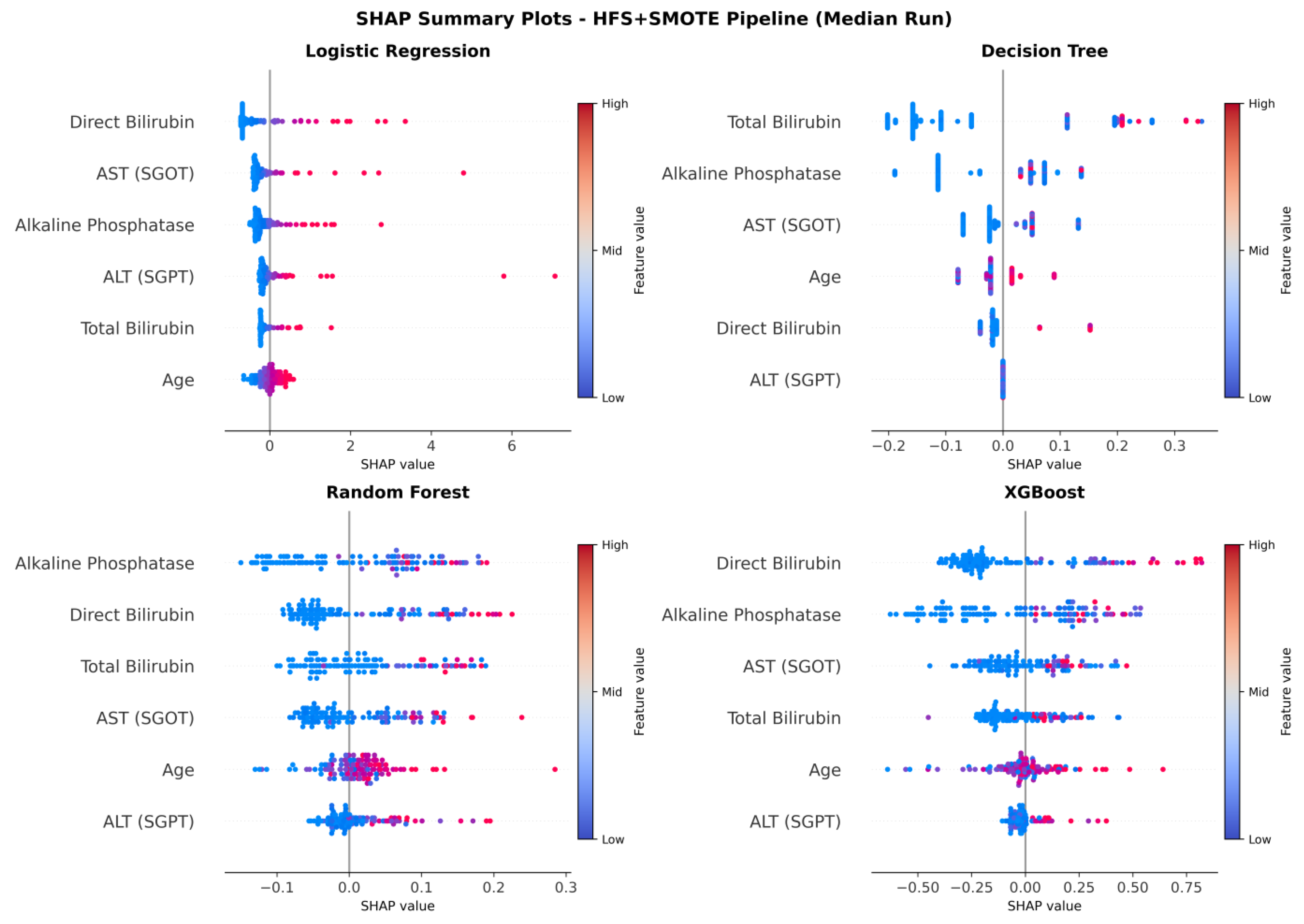
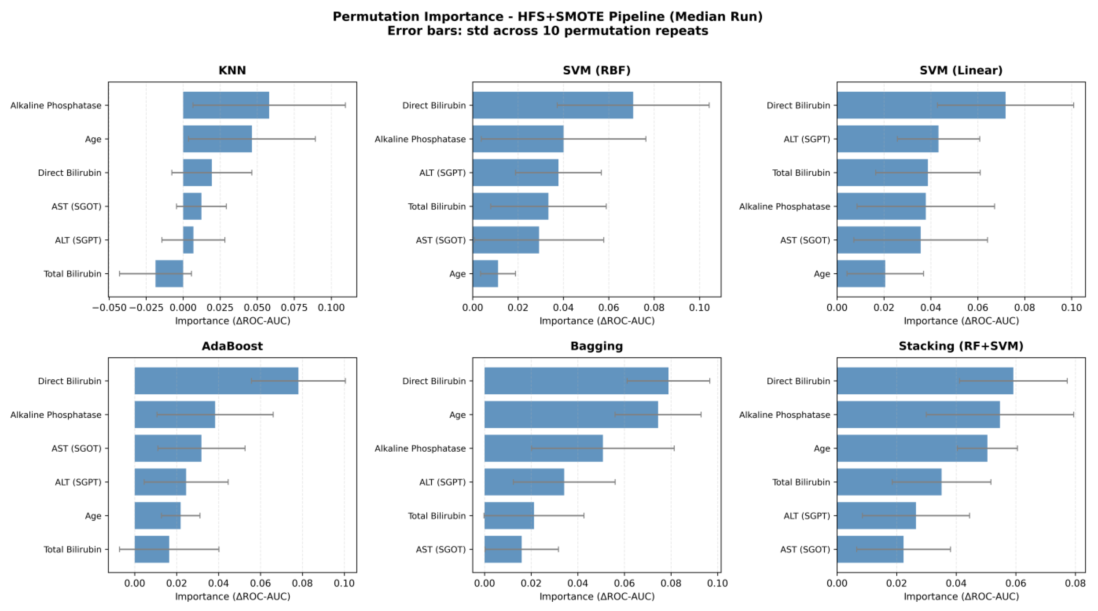
Model performance was assessed using six evaluation metrics: Accuracy, Precision, Recall, Specificity, F1-score, and the Area Under the Receiver Operating Characteristic Curve (AUC-ROC). In the context of liver disease prediction, Recall and AUC-ROC are of particular clinical significance, as they directly reflect sensitivity to true disease cases and the overall discriminative capability of the model, respectively. Additionally, confusion matrices, ROC curves, and feature importance plots were generated to support model interpretation. For feature importance analysis, the explainability method was selected according to the internal architecture of each classifier. Specifically, SHAP (SHapley Additive exPlanations) was applied to models with well-defined internal representations: LinearExplainer was used for Logistic Regression, TreeExplainer for Random Forest, and the general Explainer for Decision Tree and XGBoost. These explainers access the model’s internal parameters directly, yielding theoretically grounded and low-variance importance estimates. For the remaining models—KNN, SVM-RBF, SVM-Linear, AdaBoost, Bagging, and Stacking—SHAP is either computationally prohibitive or architecturally incompatible due to the absence of tree structures or linear parameters. Consequently, Permutation Importance was applied to these models, as it is a model-agnostic method that quantifies feature contribution by measuring the degradation in predictive performance upon randomly permuting each feature’s values. This dual-method strategy ensures that all classifiers are evaluated with the most appropriate and reliable explainability technique available [54,55]. The following terms help in calculating these metrics, which are given in Equations (8)–(12):

True Positive (TP)—when positive values are predicted as positive.

True Negative (TN)—when negative values are predicted as negative.

False Positive (FP)—when negative values are predicted as positive.

False Negative (FN)—when positive values are predicted as negative.

$$Accuracy={\displaystyle \frac{TP+TN}{TP+TN+FP+FN}}$$

(8)

$$Precision={\displaystyle \frac{TP}{TP+FP}}$$

(9)

$$Recall={\displaystyle \frac{TP}{TP+FN}}$$

(10)

$$F1-score={\displaystyle \frac{2\times (Precision\times Recall)}{(Precision+Recall)}}$$

(11)

$$Specificity={\displaystyle \frac{TN}{TN+FP}}$$

(12)

3.8. Repeated Train-Test Split Validation and Statistical Testing

To rigorously characterize the variance induced by the choice of train-test partition and to enable formal statistical comparison between the two pipelines, the entire experimental procedure—including imputation, scaling, HFS feature selection, SMOTE resampling, GridSearchCV hyperparameter optimization, 10-fold cross-validation, and test-set evaluation—was repeated ten times with independent train-test splits (random_state = 0, 1, …, 9). All internal random states (HFS, SMOTE, classifiers, and GridSearchCV cross-validation splitter) were held constant at 42 across runs, ensuring that observed performance variability could be attributed exclusively to the train-test partition. For each model and each performance metric, the mean and standard deviation across the ten runs are reported. To assess whether the performance differences between the without-HFS configuration and the HFS + SMOTE configuration are statistically significant rather than artifacts of the particular split, paired Wilcoxon signed-rank tests were applied to the ten paired ROC-AUC values per model, with $\alpha =0.05$ as the significance threshold. The Wilcoxon test was selected over the parametric paired t-test because it does not require the assumption of normality in the difference distribution, which is rarely satisfied with small sample sizes (n = 10). For explainability analysis (SHAP and Permutation Importance), the median-performance run—defined as the run where the HFS + SMOTE configuration means the ROC-AUC across all classifiers was closest to the global median—was selected as a representative case to avoid arbitrary selection bias.

3.9. Computational Complexity

The computational complexity of the HFS algorithm comprises four stages. Stage 1 (Pearson redundancy elimination) computes pairwise correlations for all $d(d-1)/2$ feature pairs, each requiring $O(n)$ time, yielding $O(n{d}^2)$ for this stage; for ILPD (d = 10), this produces 45 pairwise comparisons. Stage 2 (Information Gain and Gain Ratio estimation) computes mutual information for each non-redundant feature at a cost of $O(n)$ per feature, yielding $O(nd)$. Stage 3 (hybrid scoring) is $O(d)$, and the subsequent ranking step is $O(d\mathit{log}d)$. The total complexity is therefore

$$O(n{d}^2+nd+d\mathit{log}d)\approx O(n{d}^2)$$

(13)

For datasets where $n>>d$ (as in ILPD, where n = 583 and d = 10), the $d^2$ term is negligible, and the practical runtime is dominated by the $O(nd)$ mutual information estimation, making the algorithm highly efficient relative to wrapper or embedded methods that require repeated model training. By reducing the feature dimensionality from d to k prior to model training, the HFS framework further decreases the input space of downstream classifiers, proportionally reducing both training time and memory requirements.

4. Results

This section presents the results of the leakage-free experimental protocol described in Section 3. All performance metrics are reported as mean ± standard deviation across ten independent train-test splits. The statistical significance of pipeline improvements was assessed using paired Wilcoxon signed-rank tests on per-run ROC-AUC values, with p-values reported alongside Δ ROC-AUC. The HFS feature selection frequency analysis, explainability results from the median-performance run, and aggregate confusion matrix behavior are also presented to provide a comprehensive picture of pipeline performance.

4.1. Performance Comparison Across Ten Independent Runs

Table 5. Performance metrics of ten classifiers without HFS, reported as mean ± standard deviation across ten independent train-test splits.

Model	Accuracy	Precision	Recall	Specificity	F1 Score	ROC-AUC
KNN	0.660 ± 0.033	0.737 ± 0.016	0.808 ± 0.053	0.297 ± 0.063	0.771 ± 0.028	0.634 ± 0.059
SVM (RBF)	0.679 ± 0.036	0.725 ± 0.028	0.890 ± 0.092	0.165 ± 0.168	0.796 ± 0.032	0.665 ± 0.038
SVM (Linear)	0.709 ± 0.000	0.709 ± 0.000	1.000 ± 0.000	0.000 ± 0.000	0.830 ± 0.000	0.694 ± 0.042
XGBoost	0.685 ± 0.035	0.741 ± 0.025	0.855 ± 0.059	0.268 ± 0.120	0.793 ± 0.027	0.715 ± 0.047
Decision Tree	0.659 ± 0.035	0.747 ± 0.046	0.804 ± 0.135	0.306 ± 0.246	0.765 ± 0.049	0.668 ± 0.048
Stacking (RF + SVM)	0.703 ± 0.021	0.716 ± 0.010	0.965 ± 0.037	0.065 ± 0.058	0.822 ± 0.015	0.726 ± 0.048
Bagging	0.685 ± 0.040	0.752 ± 0.028	0.833 ± 0.051	0.326 ± 0.098	0.789 ± 0.030	0.728 ± 0.043
Random Forest	0.694 ± 0.024	0.739 ± 0.009	0.880 ± 0.053	0.241 ± 0.065	0.802 ± 0.021	0.736 ± 0.047
AdaBoost	0.705 ± 0.039	0.746 ± 0.036	0.892 ± 0.070	0.250 ± 0.170	0.810 ± 0.028	0.717 ± 0.062
Logistic Regression	0.704 ± 0.032	0.737 ± 0.018	0.906 ± 0.044	0.212 ± 0.077	0.813 ± 0.023	0.740 ± 0.040

and

Table 6. Performance metrics of ten classifiers with HFS + SMOTE, reported as mean ± standard deviation across ten independent train-test splits.

Model	Accuracy	Precision	Recall	Specificity	F1 Score	ROC-AUC
KNN	0.629 ± 0.050	0.853 ± 0.054	0.578 ± 0.060	0.753 ± 0.104	0.688 ± 0.049	0.719 ± 0.053
SVM (RBF)	0.568 ± 0.042	0.922 ± 0.027	0.429 ± 0.067	0.909 ± 0.038	0.582 ± 0.060	0.743 ± 0.031
SVM (Linear)	0.567 ± 0.052	0.931 ± 0.049	0.420 ± 0.071	0.924 ± 0.056	0.576 ± 0.069	0.748 ± 0.036
XGBoost	0.690 ± 0.041	0.823 ± 0.049	0.723 ± 0.072	0.609 ± 0.148	0.766 ± 0.037	0.741 ± 0.053
Decision Tree	0.626 ± 0.055	0.842 ± 0.022	0.583 ± 0.096	0.729 ± 0.069	0.684 ± 0.068	0.693 ± 0.034
Stacking (RF + SVM)	0.694 ± 0.038	0.827 ± 0.032	0.720 ± 0.045	0.629 ± 0.077	0.769 ± 0.032	0.746 ± 0.043
Bagging	0.700 ± 0.063	0.825 ± 0.037	0.731 ± 0.076	0.624 ± 0.083	0.774 ± 0.054	0.747 ± 0.042
Random Forest	0.692 ± 0.041	0.842 ± 0.048	0.701 ± 0.050	0.671 ± 0.126	0.763 ± 0.033	0.750 ± 0.044
AdaBoost	0.649 ± 0.040	0.850 ± 0.046	0.616 ± 0.049	0.729 ± 0.096	0.712 ± 0.037	0.727 ± 0.061
Logistic Regression	0.613 ± 0.038	0.885 ± 0.028	0.522 ± 0.049	0.835 ± 0.044	0.656 ± 0.042	0.746 ± 0.034

summarize the predictive performance of all ten classifiers under both experimental conditions, aggregated across ten independent train-test splits.

Table 7. Statistical comparison of ROC-AUC between the two pipelines using paired Wilcoxon signed-rank tests on per-run values (n = 10). Δ ROC-AUC = mean(with HFS) − mean(without HFS). * indicates p < 0.05.

Model	ROC-AUC (Without HFS)	ROC-AUC (with HFS)	Δ ROC-AUC	p-Value
KNN	0.6342 ± 0.0556	0.7192 ± 0.0500	+0.0850	0.0273 *
SVM (RBF)	0.6649 ± 0.0362	0.7432 ± 0.0293	+0.0783	0.0020 *
SVM (Linear)	0.6938 ± 0.0395	0.7479 ± 0.0339	+0.0541	0.0098 *
XGBoost	0.7148 ± 0.0446	0.7415 ± 0.0499	+0.0266	0.0137 *
Decision Tree	0.6676 ± 0.0460	0.6928 ± 0.0324	+0.0252	0.0488 *
Stacking (RF + SVM)	0.7260 ± 0.0456	0.7461 ± 0.0407	+0.0201	0.1055
Bagging	0.7284 ± 0.0407	0.7475 ± 0.0402	+0.0190	0.0645
Random Forest	0.7356 ± 0.0444	0.7500 ± 0.0416	+0.0144	0.3750
AdaBoost	0.7166 ± 0.0585	0.7274 ± 0.0581	+0.0108	0.2324
Logistic Regression	0.7405 ± 0.0379	0.7456 ± 0.0322	+0.0051	0.4413

Bold values indicate statistically significant improvements, where the ROC-AUC difference (ΔROC-AUC) is positive and the Wilcoxon signed-rank test p-value is below 0.05.

reports the corresponding statistical comparison of ROC-AUC values via paired Wilcoxon signed-rank tests. The results reveal two distinct phenomena. First, the HFS + SMOTE pipeline produced statistically significant ROC-AUC improvements (p < 0.05) in five of the ten classifiers: KNN (Δ = +0.085, p = 0.027), SVM-RBF (Δ = +0.078, p = 0.002), SVM-Linear (Δ = +0.054, p = 0.010), XGBoost (Δ = +0.027, p = 0.014), and Decision Tree (Δ = +0.025, p = 0.049). The remaining five classifiers showed positive but non-significant Δ ROC-AUC values, indicating that the proposed pipeline never degraded discriminative performance in any model. Second, and perhaps more clinically important, the baseline configuration (without HFS) exhibited a severe majority-class collapse: mean Specificity ranged from 0.000 (SVM-Linear, SVM-RBF) to 0.326 (Bagging), indicating that several classifiers learned to predict almost every test instance as positive. The addition of HFS + SMOTE resolved this pathology entirely, increasing Specificity into the 0.61–0.92 range across all ten classifiers. This rebalancing was accompanied by an expected reduction in Recall, reflecting a shift from a high-Sensitivity/near-zero-Specificity regime to a clinically meaningful balanced classification regime.

4.2. HFS Feature Selection Stability

The HFS framework selected k = 6 features per run, resulting in a total of 60 selection events across the ten runs. Table 2 reports the selection frequency of each candidate feature, providing a direct empirical assessment of HFS stability under variation of the train-test partition. Four features—Aspartate Aminotransferase (AST), Alanine Aminotransferase (ALT), Total Bilirubin, and Age—were selected in all ten runs (100% selection rate), forming a clinically coherent core feature set composed of two hepatic transaminases (markers of hepatocyte injury), a bilirubin metabolism indicator, and a demographic risk factor. Two additional features, Alkaline Phosphatase (7/10) and Direct Bilirubin (6/10), were selected in the majority of runs, while Gender (4/10), Albumin (2/10), and the Albumin/Globulin Ratio (1/10) were selected only sporadically. Total Proteins was never selected. This frequency profile demonstrates that the proposed HFS framework consistently identifies the most clinically informative features while exhibiting calibrated uncertainty around features of marginal discriminative power.

4.3. Explainability Analysis on the Median-Performance Run

The SHAP summary plots presented in Figure 5 reveal consistent feature importance rankings across the four tree-compatible and linear models. For Random Forest and XGBoost, Total Bilirubin and Direct Bilirubin emerged as the top contributors to model output, with high feature values associated with positive (liver disease) predictions, as indicated by the red coloring on the right side of the SHAP axis. Aspartate Aminotransferase (AST) and Alanine Aminotransferase (ALT)—the two features assigned the highest hybrid scores by HFS—exhibited moderate SHAP magnitudes in tree-based models, suggesting that while they carry high marginal information content with respect to the target, their contribution within the trained model’s decision surface is partially mediated by correlated enzymatic markers. For Logistic Regression, the SHAP analysis using LinearExplainer confirmed a near-monotonic positive association between bilirubin elevation and liver disease prediction, consistent with its biological role as a downstream marker of hepatic dysfunction. The Decision Tree exhibited a simpler importance profile, with a single split on Total Bilirubin dominating the root node, reflecting the greedy nature of univariate splitting criteria.

The Permutation Importance plots displayed in Figure 6 corroborate and extend these findings for the remaining six classifiers—KNN, SVM-RBF, SVM-Linear, AdaBoost, Bagging, and Stacking—where SHAP is architecturally incompatible or computationally prohibitive. Across all six models, AST and ALT consistently ranked among the top three features by mean importance score, with small standard deviations across the ten permutation repeats (error bars in Figure 6) indicating stable and reproducible importance estimates. Total Bilirubin retained its high importance ranking across instance-based and kernel-based learners, while Age contributed meaningfully to all models, particularly to distance-based classifiers (KNN) where its continuous numeric nature provides fine-grained separability. Notably, the Stacking ensemble exhibited the most distributed importance profile, with no single feature dominating—a pattern consistent with the complementary inductive biases of its constituent RF and SVM-RBF base learners. Taken together, the convergence of filter-based HFS rankings, SHAP attributions, and permutation-based importance estimates across ten heterogeneous classifiers provides strong multi-method validation for the clinical interpretability of the selected feature subset.

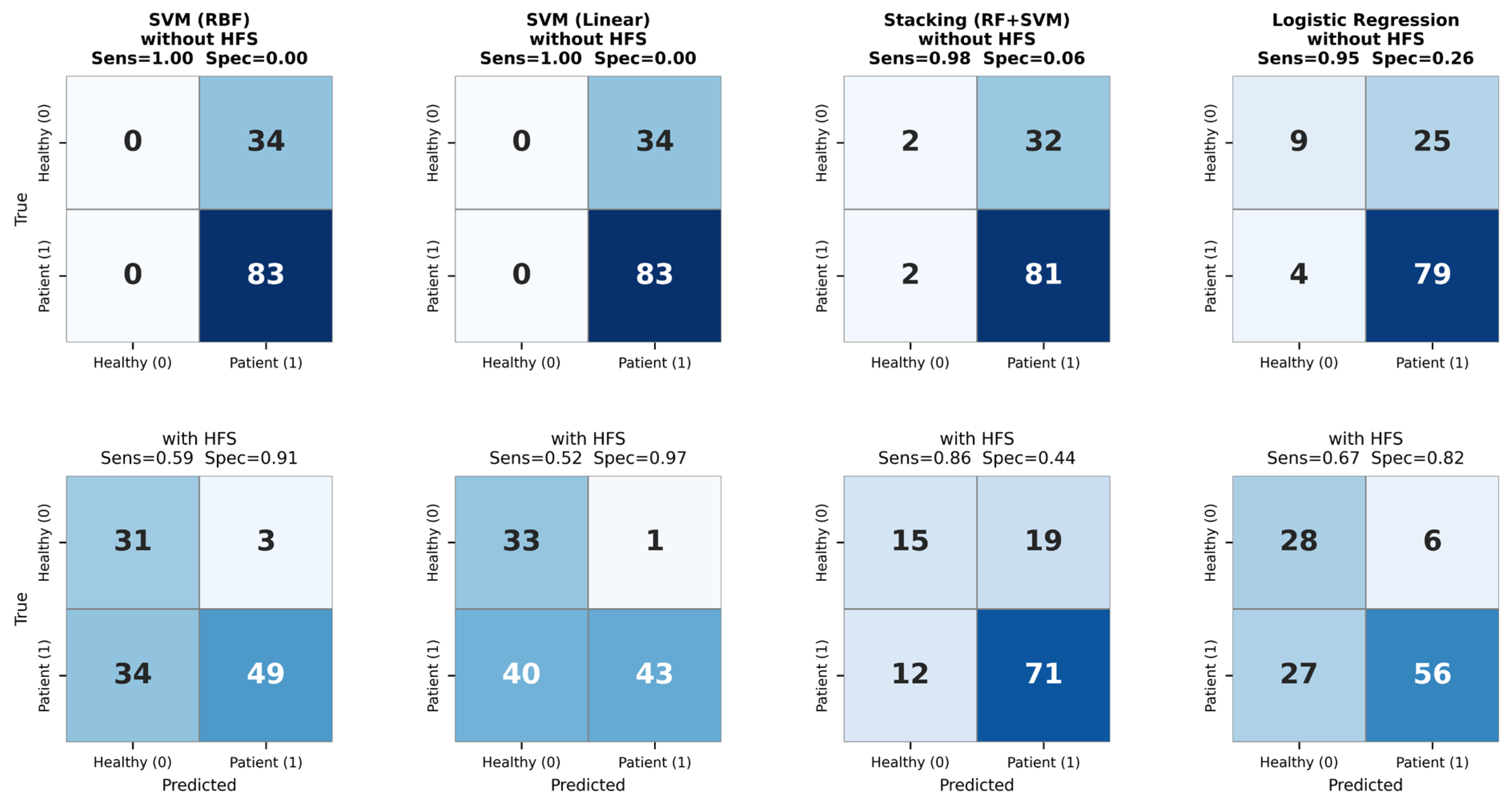
The confusion matrices displayed in Figure 7 provide a direct visual confirmation of the majority-class collapse phenomenon and its resolution. In the baseline configuration (without HFS), SVM-Linear and SVM-RBF exhibit a nearly degenerate prediction pattern: virtually all instances are assigned to the positive (liver disease) class, resulting in a true negative count of zero or near-zero and a false positive count approaching the total number of healthy controls. Stacking and Logistic Regression show a similar, if less extreme, tendency toward positive-class dominance. Under the HFS + SMOTE pipeline, the confusion matrix structure transforms markedly for all four models: true negatives increase substantially, false positives decrease, and the prediction distribution becomes genuinely bimodal. The most striking transformation is observed in SVM-Linear and SVM-RBF, where Specificity improves from 0.000 to above 0.90, at the cost of a modest reduction in true positives. This visual evidence reinforces the quantitative findings of Table 6 and underscores that the pipeline improvement is not a marginal numerical gain but a qualitative shift in classifier behavior.

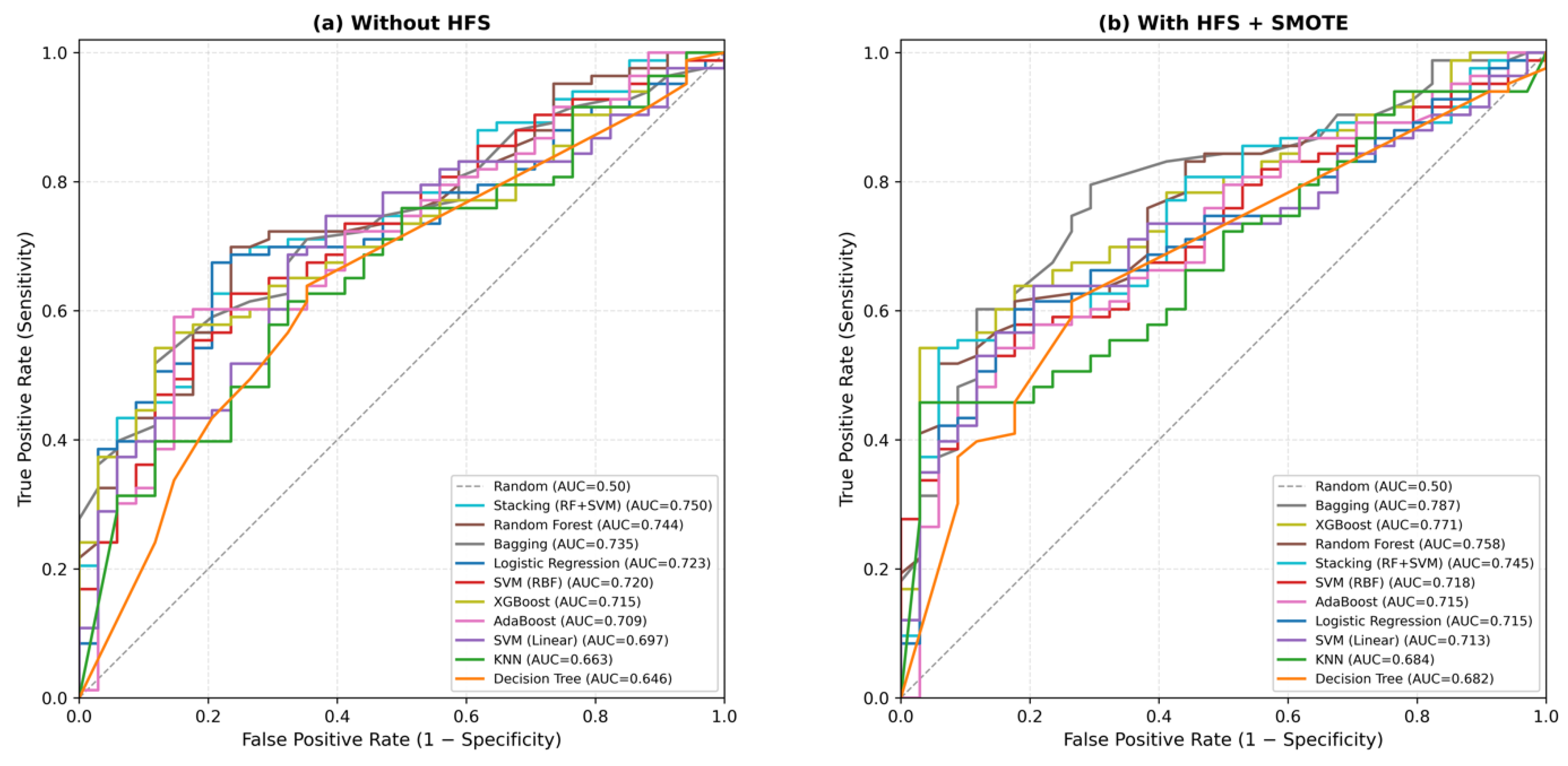
The ROC curves presented in Figure 8 illustrate the discriminative capacity of all ten classifiers under both pipeline configurations. In the without-HFS panel, curves for KNN and SVM-based models cluster near the diagonal, consistent with their low ROC-AUC values (0.63–0.69) as reported in Table 5, reflecting the poor rank-ordering of disease and non-disease cases. In the with-HFS panel, these same models shift noticeably toward the upper-left corner of the ROC space, visually confirming the statistically significant AUC gains reported in Table 7. Tree-based ensembles—Random Forest, Bagging, and Stacking—exhibit relatively stable curve positions across both panels, consistent with their smaller and non-significant Δ ROC-AUC values, reflecting their inherent robustness to input feature redundancy. Across both panels, no model falls below the diagonal, confirming that the HFS + SMOTE pipeline produced no degradation in discriminative performance for any classifier. The tightening of inter-model spread in the HFS panel further suggests that the pipeline reduces classifier sensitivity to architectural differences, producing more homogeneous and reliable discrimination across the evaluated model family.

4.4. Ablation Study: Disentangling HFS and SMOTE Contributions

To isolate the individual contributions of HFS and SMOTE, a 2 × 2 ablation study was conducted across all 10 independent train-test splits and 10 classifiers. Four pipeline configurations were evaluated: (A) Neither (full features, no SMOTE), (B) HFS + SMOTE (proposed pipeline), (C) SMOTE only (full features with SMOTE), and (D) HFS only (selected features without SMOTE).

Table 8. Ablation study results on the ILPD dataset: ROC-AUC (mean ± standard deviation) across 10 independent train-test splits for four pipeline configurations. Neither = full features without SMOTE; HFS only = selected features without SMOTE; SMOTE only = full features with SMOTE; HFS + SMOTE = proposed pipeline.

Classifier	Neither	HFS Only	SMOTE Only	HFS + SMOTE
KNN	0.6342 ± 0.0586	0.7251 ± 0.0397	0.6280 ± 0.0634	0.7192 ± 0.0527
SVM (RBF)	0.6649 ± 0.0381	0.6749 ± 0.0203	0.7434 ± 0.0458	0.7432 ± 0.0309
SVM (Linear)	0.6834 ± 0.0379	0.6259 ± 0.1298	0.7445 ± 0.0421	0.7479 ± 0.0357
XGBoost	0.7148 ± 0.0471	0.7181 ± 0.0606	0.7203 ± 0.0452	0.7415 ± 0.0526
Decision Tree	0.6676 ± 0.0485	0.6851 ± 0.0460	0.6842 ± 0.0503	0.6928 ± 0.0342
Stacking (RF + SVM)	0.7260 ± 0.0480	0.7362 ± 0.0388	0.7311 ± 0.0523	0.7461 ± 0.0429
Bagging	0.7284 ± 0.0428	0.7402 ± 0.0458	0.7318 ± 0.0506	0.7475 ± 0.0424
Random Forest	0.7356 ± 0.0468	0.7405 ± 0.0319	0.7354 ± 0.0486	0.7500 ± 0.0439
AdaBoost	0.7166 ± 0.0617	0.7245 ± 0.0610	0.7175 ± 0.0636	0.7274 ± 0.0613
Logistic Regression	0.7405 ± 0.0400	0.7429 ± 0.0336	0.7418 ± 0.0379	0.7456 ± 0.0339

Values indicate the highest ROC-AUC for each classifier across the four configurations.

presents the ROC-AUC results (mean ± standard deviation) for all configurations.

The marginal effects, computed as the average improvement attributable to each component across all classifiers, reveal that SMOTE contributes a mean ROC-AUC increase of +0.021 and HFS contributes +0.014. The interaction term is approximately zero (<0.001), indicating that the two components operate independently and their combined effect is approximately additive.

The most striking finding concerns Specificity. The baseline configuration (Neither) produces a mean Specificity of 0.214, reflecting severe majority-class collapse. SMOTE alone increases Specificity to 0.716, while HFS alone produces only a marginal change (0.207). The full pipeline (HFS + SMOTE) achieves 0.741, confirming that SMOTE is the primary driver of the Specificity transformation and HFS provides incremental refinement.

Model-specific patterns are informative. KNN benefits overwhelmingly from HFS (marginal effect: +0.091), with negligible SMOTE contribution (−0.006), consistent with its known sensitivity to the curse of dimensionality. Conversely, SVM-Linear and SVM-RBF benefit predominantly from SMOTE (+0.092 and +0.073, respectively), reflecting their sensitivity to class imbalance in margin-based optimization. Tree-based ensembles show moderate but balanced gains from both components.

4.5. Sensitivity Analysis of HFS Parameters

Two sensitivity analyses were conducted to evaluate the robustness of the HFS algorithm to its key parameters: the hybrid weight w and the number of selected features k.

4.5.1. Sensitivity to the Weighting Parameter w

The weighting parameter w controls the relative contribution of Information Gain (IG) and Gain Ratio (GR) to the hybrid score. Five values were tested: w $\in$ {0.0, 0.25, 0.50, 0.75, 1.0}, where w = 0 uses GR exclusively and w = 1 uses IG exclusively. All other parameters were held constant ($\theta =0.90$, k = 6).

Table 9. Sensitivity analysis of the weighting parameter w: ROC-AUC (mean ± standard deviation) across 10 independent train-test splits. w = 0.0 corresponds to pure Gain Ratio, w = 1.0 to pure Information Gain, and w = 0.50 (default) assigns equal weight to both measures. Fixed parameters: $\theta =0.90$, k = 6.

Classifier	w = 0.0	w = 0.25	w = 0.50	w = 0.75	w = 1.0
KNN	0.7220 ± 0.0343	0.7152 ± 0.0381	0.7192 ± 0.0527	0.7196 ± 0.0522	0.7196 ± 0.0522
SVM (RBF)	0.7339 ± 0.0423	0.7396 ± 0.0345	0.7432 ± 0.0309	0.7373 ± 0.0411	0.7373 ± 0.0411
SVM (Linear)	0.7408 ± 0.0461	0.7434 ± 0.0404	0.7479 ± 0.0357	0.7466 ± 0.0382	0.7466 ± 0.0382
XGBoost	0.7314 ± 0.0642	0.7318 ± 0.0565	0.7415 ± 0.0526	0.7384 ± 0.0572	0.7376 ± 0.0561
Decision Tree	0.6865 ± 0.0392	0.6909 ± 0.0367	0.6928 ± 0.0342	0.6985 ± 0.0333	0.6978 ± 0.0325
Stacking (RF + SVM)	0.7381 ± 0.0566	0.7403 ± 0.0492	0.7461 ± 0.0429	0.7443 ± 0.0435	0.7439 ± 0.0450
Bagging	0.7483 ± 0.0555	0.7443 ± 0.0501	0.7475 ± 0.0424	0.7476 ± 0.0432	0.7477 ± 0.0425
Random Forest	0.7470 ± 0.0591	0.7499 ± 0.0525	0.7500 ± 0.0439	0.7477 ± 0.0459	0.7533 ± 0.0499
AdaBoost	0.7190 ± 0.0580	0.7196 ± 0.0581	0.7274 ± 0.0613	0.7279 ± 0.0602	0.7279 ± 0.0602
Logistic Regression	0.7423 ± 0.0380	0.7434 ± 0.0339	0.7456 ± 0.0339	0.7445 ± 0.0360	0.7445 ± 0.0360

The overall mean ROC-AUC across all classifiers ranges from 0.731 (w = 0.0) to 0.736 (w = 0.50), a total spread of 0.005, indicating low sensitivity to the weighting parameter.

reports the results across 10 runs and 10 classifiers.

The overall mean ROC-AUC ranges from 0.731 (w = 0.0) to 0.736 (w = 0.5), a total spread of only 0.005. The default value w = 0.50 achieves the highest mean, confirming the original choice. Importantly, the core feature set (AST, ALT, Total Bilirubin) is selected in all 10 runs at every w value, demonstrating that HFS’s feature selection is robust to the weighting parameter on this dataset. The low sensitivity to w is expected, given that IG and GR are monotonically related for features with similar entropy and diverge primarily for features with highly uneven value distributions.

4.5.2. Sensitivity to the Number of Selected Features k

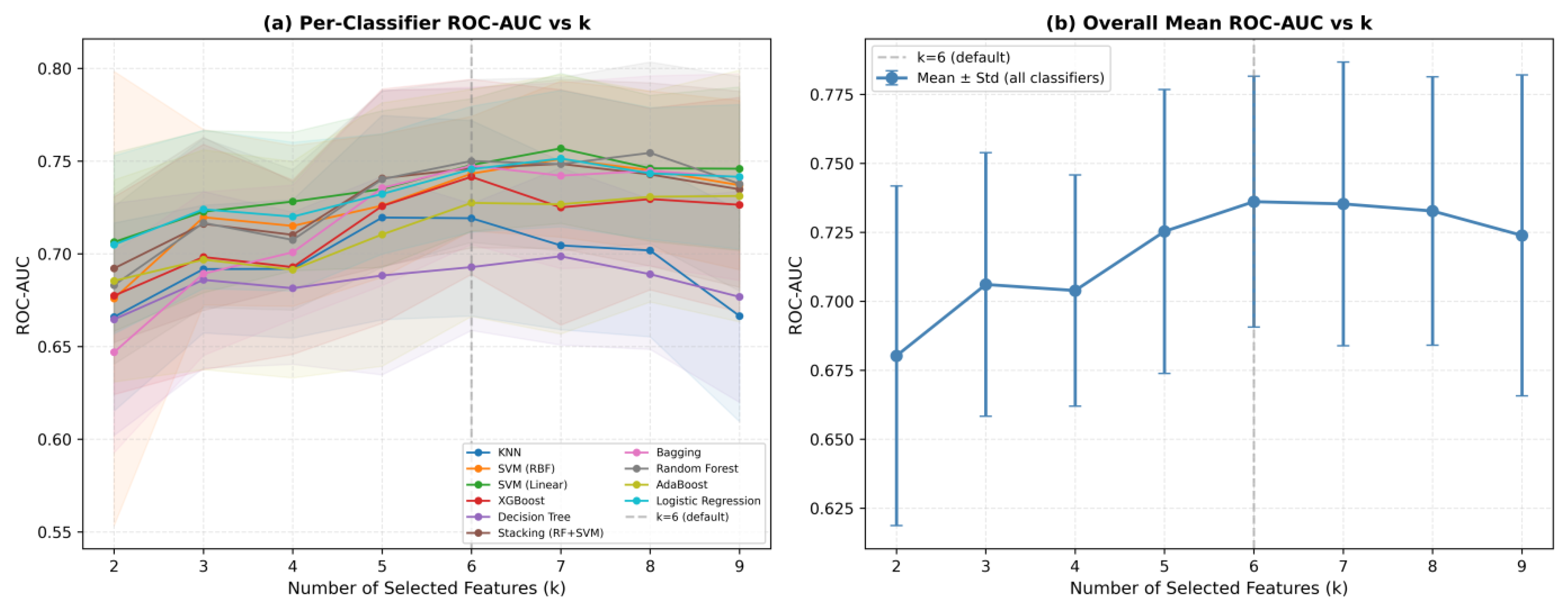
The parameter k determines how many features are retained after hybrid scoring. Eight values were tested: k $\in$ {2, 3, 4, 5, 6, 7, 8, 9}, with w = 0.50 and $\theta =0.90$ held constant. Figure 9 presents per-classifier and overall mean ROC-AUC as a function of k.

The overall mean ROC-AUC exhibits a clear inverted-U pattern: performance increases monotonically from k = 2 (0.680) to k = 6 (0.736), then declines toward k = 9 (0.724). This pattern reflects the classical bias-variance trade-off: too few features (k = 2–3) result in underfitting due to insufficient information, while too many features (k = 8–9) reintroduce noisy or weakly informative attributes. The standard deviation also narrows at k = 6, indicating more stable performance across classifiers. These results confirm k = 6 as the empirically optimal choice for the ILPD dataset.

At the model level, KNN shows the steepest decline beyond k = 6 (from 0.719 at k = 6 to 0.666 at k = 9), consistent with its known sensitivity to irrelevant dimensions. Linear models (SVM-Linear, Logistic Regression) peak at k = 7, maintaining near-optimal performance across a wider range. Tree-based ensembles exhibit the flattest profiles, consistent with their built-in feature selection mechanisms.

4.6. Generalizability Assessment on BUPA Liver Disorders

To assess the generalizability of the proposed pipeline, the full experimental protocol was replicated on the BUPA Liver Disorders dataset (Section 3.2).

Table 10. Ablation study results on the BUPA Liver Disorders dataset: ROC-AUC (mean ± standard deviation) across 10 independent train-test splits. Target variable: drinks ≥ 3 (Forsyth method). HFS parameters: $\theta =0.90$, w = 0.50, k = 3. No paired Wilcoxon test reached significance at p < 0.05 for any classifier.

Classifier	Neither	HFS only	SMOTE only	HFS + SMOTE
KNN	0.5986 ± 0.0795	0.5839 ± 0.0827	0.5983 ± 0.0735	0.5762 ± 0.0695
SVM (RBF)	0.5959 ± 0.0615	0.6091 ± 0.0672	0.5955 ± 0.0610	0.6189 ± 0.0645
SVM (Linear)	0.6348 ± 0.0771	0.6297 ± 0.0645	0.6341 ± 0.0843	0.6356 ± 0.0668
XGBoost	0.6029 ± 0.0758	0.5916 ± 0.0579	0.6022 ± 0.0766	0.5892 ± 0.0603
Decision Tree	0.5619 ± 0.0652	0.5594 ± 0.0746	0.5582 ± 0.0753	0.5410 ± 0.0634
Stacking (RF + SVM)	0.6062 ± 0.0743	0.5865 ± 0.0700	0.6146 ± 0.0743	0.5886 ± 0.0707
Bagging	0.5862 ± 0.0763	0.5716 ± 0.0790	0.5864 ± 0.0786	0.5768 ± 0.0817
Random Forest	0.5912 ± 0.0795	0.5810 ± 0.0653	0.5925 ± 0.0744	0.5839 ± 0.0678
AdaBoost	0.5606 ± 0.0685	0.5807 ± 0.0569	0.5672 ± 0.0680	0.5838 ± 0.0601
Logistic Regression	0.6356 ± 0.0738	0.6334 ± 0.0616	0.6366 ± 0.0772	0.6336 ± 0.0612

The near-perfect class balance of BUPA (51%/49%) and absence of redundant feature pairs at $\theta =0.90$ explain the negligible effect of both SMOTE and HFS redundancy elimination on this dataset.

presents the 2 × 2 ablation results for BUPA.

Unlike ILPD, the HFS + SMOTE pipeline did not produce statistically significant improvements on BUPA. No paired Wilcoxon test reached significance at p < 0.05 for any classifier. The best-performing model (SVM-Linear) achieved ROC-AUC = 0.636 ± 0.067, considerably lower than the ILPD equivalent (0.748 ± 0.036).

This null result is both expected and informative. BUPA differs from ILPD in two critical respects: (1) near-perfect class balance (51%/49%), which renders SMOTE unnecessary, and (2) no feature pairs exceeding the redundancy threshold $\theta =0.90$, which eliminates the benefit of Stage 1 redundancy filtering. The ablation confirms these mechanisms: the SMOTE-only configuration produces near-identical results to the baseline (mean difference < 0.001 across all classifiers), consistent with the absence of class imbalance. Similarly, the HFS-only configuration shows mixed effects, with some classifiers improving marginally and others declining, reflecting the information loss from discarding two of five features without corresponding noise reduction.

This finding confirms that the HFS + SMOTE pipeline’s effectiveness on ILPD is mechanistically linked to the presence of class imbalance and feature redundancy. When these conditions are absent, the pipeline appropriately converges to baseline performance. The contrast between ILPD and BUPA strengthens the generalizability claim by demonstrating that the observed improvements are not artifacts of benchmark-specific overfitting but rather principled responses to dataset characteristics.

4.7. Explainability Stability Across Independent Runs

To assess the stability of feature importance rankings, SHAP and Permutation Importance were computed across all 10 independent train-test partitions.

Table 11. Feature importance rank stability across 10 independent train-test splits (ILPD dataset). Each cell reports the mean rank ± standard deviation (rank 1 = most important). The Consensus column shows the mean rank averaged across all 10 classifiers. Features are ordered by consensus rank. LR = Logistic Regression; DT = Decision Tree; RF = Random Forest; XGB = XGBoost; SVM-R = SVM (RBF); SVM-L = SVM (Linear); AdaB = AdaBoost; Bag = Bagging; Stack = Stacking (RF + SVM). SHAP-based importance was used for LR, DT, RF, and XGB; permutation importance for the remaining classifiers.

Feature	LR	DT	RF	XGB	KNN	SVM-R	SVM-L	AdaB	Bag	Stack	Consensus
Direct Bilirubin	1.3 ± 0.5	2.2 ± 1.8	1.7 ± 0.5	1.3 ± 0.8	3.0 ± 1.4	1.3 ± 0.5	1.2 ± 0.4	2.2 ± 1.6	2.2 ± 1.2	2.3 ± 1.5	1.87
Alk. Phosphatase	3.9 ± 1.2	2.1 ± 0.4	1.1 ± 0.4	2.6 ± 1.1	1.9 ± 0.7	2.7 ± 1.6	2.7 ± 1.5	3.9 ± 1.8	3.3 ± 0.8	3.3 ± 1.0	2.75
ALT (SGPT)	2.4 ± 1.1	3.6 ± 1.4	3.9 ± 1.2	3.7 ± 1.3	4.0 ± 1.3	2.9 ± 1.0	3.1 ± 1.3	2.4 ± 1.1	2.6 ± 1.7	2.8 ± 1.8	3.14
Total Bilirubin	3.3 ± 1.8	2.1 ± 1.5	2.7 ± 1.1	3.3 ± 1.6	4.7 ± 1.7	3.1 ± 1.6	2.7 ± 1.6	3.2 ± 1.9	3.7 ± 2.0	3.2 ± 1.9	3.20
Age	4.6 ± 1.2	3.7 ± 0.8	4.3 ± 1.1	2.5 ± 1.2	1.7 ± 1.3	3.9 ± 2.0	4.8 ± 1.0	3.0 ± 1.3	2.5 ± 0.8	2.6 ± 1.2	3.36
AST (SGOT)	3.1 ± 1.4	4.2 ± 0.9	4.1 ± 1.4	4.7 ± 0.9	4.5 ± 1.0	4.5 ± 1.0	3.7 ± 1.2	4.8 ± 1.4	4.5 ± 1.4	5.0 ± 1.2	4.31
A/G Ratio	5.0 ± 0.0	5.0 ± 0.0	6.0 ± 0.0	6.0 ± 0.0	3.0 ± 0.0	6.0 ± 0.0	6.0 ± 0.0	4.0 ± 0.0	6.0 ± 0.0	6.0 ± 0.0	5.30
Albumin	6.0 ± 0.0	6.0 ± 0.0	6.0 ± 0.0	6.0 ± 0.0	5.0 ± 1.4	5.5 ± 0.7	5.5 ± 0.7	5.0 ± 1.4	6.0 ± 0.0	4.5 ± 2.1	5.55
Gender	6.0 ± 0.0	5.8 ± 0.5	6.0 ± 0.0	6.0 ± 0.0	4.2 ± 1.7	5.5 ± 0.6	6.0 ± 0.0	5.5 ± 0.6	5.8 ± 0.5	5.5 ± 0.6	5.63

The consensus top-6 features (Direct Bilirubin through Age) correspond exactly to the HFS selection at k = 6, providing independent validation of the feature selection from an explainability perspective.

reports the mean importance rank ± standard deviation for each (model, feature) combination.

The consensus ranking across all 10 models identifies Direct Bilirubin as the most important feature (mean rank: 1.87), followed by Alkaline Phosphatase (2.74), ALT (3.14), Total Bilirubin (3.20), Age (3.36), and AST (4.31). Gender (5.62), Albumin (5.55), and A/G Ratio (5.30) consistently rank last. Notably, the consensus top-six features correspond exactly to HFS’s selection at k = 6, providing independent validation of the feature selection from an explainability perspective.

Rank stability varies by feature. Direct Bilirubin (std = 1.03), Gender (std = 0.44), and Albumin (std = 0.64) show the lowest variability, indicating stable importance across partitions. Total Bilirubin exhibits the highest variability (std = 1.66), ranging from rank 1 to rank 6 depending on the model and partition. This variability is clinically plausible: bilirubin levels have heterogeneous predictive value across liver disease subtypes and severity stages.

5. Discussion

The results presented in Section 4 support three principal conclusions, each of which addresses a distinct aspect of the methodological gaps identified in the literature review.

5.1. Statistical Significance of Pipeline Improvements

By repeating the entire experimental protocol ten times with independent train-test partitions and applying paired Wilcoxon signed-rank tests, this study moves beyond the single-split reporting that characterizes much of the prior ILPD literature. The observation that five of ten classifiers exhibit statistically significant ROC-AUC improvements (p < 0.05) under HFS + SMOTE—with the remaining five showing positive but non-significant trends—provides a more nuanced and credible characterization of the pipeline’s contribution than typical single-run comparisons. The largest absolute improvements occurred in classifiers that are most sensitive to the input feature geometry: KNN (Δ = +0.085, p = 0.027), SVM-RBF (Δ = +0.078, p = 0.002), and SVM-Linear (Δ = +0.054, p = 0.010). Tree-based ensembles (Random Forest, AdaBoost, Bagging, Stacking), which inherently perform internal feature selection at each split, derived smaller and statistically non-significant marginal benefits from external feature selection, consistent with prior observations that the value of feature selection diminishes in proportion to the implicit feature-selection capacity of the underlying learner. Logistic Regression—the model with the strongest internal regularization and the simplest decision surface—was the least affected (Δ = +0.005, p = 0.441), indicating that linear models with effective regularization are largely robust to the presence of redundant or irrelevant features. The ablation and explainability analyses reveal distinct complementarity patterns across classifier families. Linear models (Logistic Regression, SVM-Linear) are most sensitive to class imbalance, with SMOTE marginal effects of +0.020 to +0.092 on ROC-AUC, but are relatively insensitive to feature redundancy (HFS marginal effect: +0.003 to −0.027). This is consistent with their reliance on linear decision boundaries, which are severely biased by skewed class priors but less affected by correlated input dimensions. Distance-based models (KNN) exhibit the opposite pattern: HFS provides the largest marginal improvement (+0.091), while SMOTE has a negligible effect (−0.006), reflecting KNN’s known vulnerability to the curse of dimensionality and relative robustness to class imbalance via local neighborhood voting. Tree-based ensembles (Random Forest, XGBoost, Bagging) show moderate but balanced improvement from both components, consistent with their built-in feature selection and bootstrapping mechanisms. The Stacking ensemble (RF + SVM) achieves the most consistent improvement across all configurations, capturing the complementary strengths of its base learners. These patterns suggest that the optimal pipeline configuration is model-dependent: distance-based classifiers benefit primarily from feature selection, linear classifiers from resampling, and ensemble methods from their combination.

5.2. Resolution of Majority-Class Collapse

Beyond the moderate ROC-AUC gains, the most clinically consequential effect of the proposed pipeline lies in the resolution of majority-class collapse. In the baseline configuration (without HFS), several classifiers—most strikingly SVM-RBF and SVM-Linear (Specificity = 0.000), Stacking (Specificity = 0.065), and AdaBoost (Specificity = 0.250)—learned to predict almost every instance as positive (liver disease). While such models achieve deceptively high Recall (0.85–1.00), they provide no diagnostic discriminative power: every patient is classified as a case. In a screening context, this would translate to a 100% false-positive rate among healthy individuals, defeating the purpose of automated risk stratification. The HFS + SMOTE configuration addressed this pathology in every model, raising Specificity into the 0.61–0.92 range. The trade-off—a corresponding decline in Recall—reflects the move from a degenerate “predict-all-positive” regime to a balanced classification regime that genuinely distinguishes between disease and non-disease cases. From a clinical screening perspective, this represents a qualitatively different (and superior) operating point, even when the aggregate ROC-AUC differs only modestly. The relative contributions of HFS and SMOTE to this transformation are quantified in the ablation study (Section 4.4), which confirms that SMOTE is the primary driver of the Specificity improvement (0.214 → 0.716), while HFS provides incremental refinement (0.716 → 0.741). An important observation is that the HFS + SMOTE pipeline improves ROC-AUC while simultaneously decreasing mean Accuracy and F1-score relative to the baseline. This apparent paradox is resolved by examining the Specificity transformation. Without HFS + SMOTE, most classifiers default to near-universal positive prediction, achieving high Accuracy (driven by the 71.4% majority class) but near-zero Specificity (mean: 0.214 across all classifiers). The HFS + SMOTE pipeline rebalances the decision boundary, dramatically increasing Specificity from 0.214 to 0.741 at the cost of reduced Sensitivity. Because Accuracy and F1-score are dominated by the majority class in imbalanced settings, they mechanically decrease even though the classifier is now detecting both classes effectively. ROC-AUC, being threshold-independent and equally sensitive to both classes, better captures this improvement. The ablation study (Section 4.4 provides direct evidence: SMOTE alone drives the Specificity transformation from 0.214 to 0.716, confirming that the observed Accuracy/F1 decrease is a consequence of correcting the majority-class collapse rather than a genuine degradation in predictive capability. In clinical practice, a classifier that identifies both diseased and healthy patients (balanced Sensitivity and Specificity) is far more useful than one that labels all patients as diseased (high Accuracy but zero Specificity), even if the latter yields numerically higher Accuracy.

5.3. Filter-Based Selection vs. Model-Based Importance

A particularly informative finding emerges from comparing the HFS feature ranking with the post hoc SHAP and Permutation Importance analyses. HFS—operating purely on information-theoretic relevance—assigned the highest scores to AST and ALT, the two transaminases that were selected in all ten runs. However, in the SHAP analyses of Random Forest and XGBoost, AST and ALT received only moderate importance scores, while Bilirubin (Direct or Total) and Alkaline Phosphatase consistently dominated the top ranks. This divergence is not a contradiction but a methodologically meaningful observation: filter-based selection identifies features with high marginal information content with respect to the target, while model-based importance reflects the actual use of features within the trained model’s decision surface. The implication is that HFS may be most effective as a feature elimination tool—identifying which features to discard with high confidence—rather than as a tool for assigning fine-grained feature priorities. This interpretation is supported by the high stability of the four consistently selected features across all ten runs and the calibrated uncertainty around features of borderline relevance. Future work should explore hybrid frameworks that combine filter-based pre-screening with embedded or wrapper-based fine-ranking.

5.4. Clinical Plausibility of the Selected Feature Set

The four core features identified by HFS—AST, ALT, Total Bilirubin, and Age—are the foundational components of standard liver function testing. AST and ALT directly reflect hepatocellular injury, with their elevation indicating acute or chronic hepatic damage. Total Bilirubin captures impairment of bilirubin metabolism and conjugation, a downstream marker of advanced hepatic dysfunction. Age serves as a non-modifiable epidemiological risk factor consistent with the well-documented increase in liver disease prevalence with advancing age. The two majority-selected features—Alkaline Phosphatase (a biliary tract marker) and Direct Bilirubin (a more specific indicator of conjugated bilirubin elevation)—further reinforce the clinical coherence of the selected subset. The fact that the proposed HFS framework, operating without any domain-specific prior knowledge, converged on this clinically grounded feature set supports the validity of information-theoretic relevance scoring as a domain-agnostic feature selection strategy in biomedical applications.

5.5. Comparison with the Prior Literature

The mean ROC-AUC values reported here (0.69–0.75 with HFS + SMOTE) are notably lower than several headline figures in the recent ILPD literature, which have reported accuracies above 90% (e.g., [15,16]). Several factors contribute to this discrepancy. First, the present study employs a strictly leakage-free pipeline in which SMOTE is integrated within ImbPipeline and applied independently to each cross-validation fold, while several prior studies apply SMOTE to the full dataset prior to splitting—a practice known to inflate performance estimates by allowing test-set information to influence training. Second, the present results are averaged across ten independent train-test splits with reported standard deviations rather than a single optimistic split. Third, hyperparameter tuning in this study was performed exclusively within the training partition of each split, while some prior studies tune on the full dataset. Considered together, the present results may be interpreted as a more honest, reproducible estimate of the achievable performance on ILPD under rigorous experimental controls. The qualitative finding—that careful feature selection combined with class-balancing meaningfully improves classifier behavior on this benchmark—remains consistent with the broader literature, even when the absolute numbers are more conservative.

To contextualize the present results within the broader landscape of ILPD-based liver disease prediction research,

Table 12. Comparison of recent machine learning studies on the ILPD benchmark and closely related liver disease classification tasks (2020–2026). Reported metric values are taken from each study as published.

Study	Year	Dataset	Best Model	Metric	Value
Kuzhippallil et al. [41]	2020	ILPD	XGBoost (genetic-algorithm tuned)	Accuracy	0.881
Gupta et al. [1]	2022	ILPD	Random Forest	Accuracy	0.751
Anthonysamy and Babu [2]	2023	ILPD	MLP + Voting Classifier	Accuracy	0.889
Dritsas and Trigka [10]	2023	ILPD	Voting (RF + SVM + kNN)	Accuracy	0.801
Md et al. [14]	2023	ILPD	Extra Trees + ensemble	Accuracy	0.918
Mohamed et al. [15]	2024	ILPD	Two-Level Stacking Ensemble	Accuracy	0.940
Ganie and Pramanik [16]	2024	ILPD + LDPD	CatBoost (boosting comparison)	Accuracy	0.988
Rani et al. [11]	2025	ILPD + BUPA	SMOTEENN-KNN/SMOTEENN-AdaBoost	Accuracy	0.932
İlter and Kırelli [7]	2025	ILPD	Logistic Regression	Accuracy	0.800
Khan et al. [25]	2026	1700-record dataset	ML + Explainable AI framework	Accuracy	0.9088
Mithu et al. [8]	2026	ILPD	Interpretable ML	Accuracy	0.7133
Proposed	2026	ILPD	HFS + SMOTE + Stacking (RF + SVM)	Accuracy	0.694 ± 0.038
				ROC-AUC *	0.746 ± 0.041

Note: Reported metrics vary across studies due to differences in evaluation protocols, class definitions, and train-test strategies. Direct numerical comparison across studies should be interpreted with caution. Cells report the metric as published in each original study. * The proposed model reports ROC-AUC (mean ± standard deviation across ten independent train-test splits) rather than Accuracy. ROC-AUC is preferred under class imbalance because it captures classifier ranking quality independently of decision threshold and is not inflated by majority-class prediction. Direct numerical comparison with single-split Accuracy values reported in prior studies should therefore be interpreted with caution. The reported value corresponds to the Stacking (RF + SVM) classifier—see Table 6 for the complete set of ten classifier results.

summarizes ten representative studies published between 2020 and 2026, covering classical ensembles, boosting algorithms, hybrid resampling pipelines, and recent explainable-AI-integrated frameworks. Most prior studies report Accuracy as the primary metric on the ILPD benchmark, with values ranging from 0.75 to 0.99. The proposed framework departs from this convention in three respects: (i) ROC-AUC is reported as the primary metric rather than Accuracy, since ROC-AUC is more robust under class imbalance and is not inflated by majority-class prediction; (ii) results are reported as the mean ± standard deviation across ten independent train-test splits rather than as a single optimistic value; and (iii) SMOTE is integrated within an ImbPipeline so that resampling is applied independently within each cross-validation fold, preserving the integrity of the held-out test set. These methodological choices yield more conservative numerical values but provide a more reproducible and statistically defensible performance estimate. The clinical significance of this distinction is illustrated by a concrete example from the surveyed literature: İlter and Kırelli [7]—using the same ILPD benchmark without class balancing—reported LR as the best-performing model at 80% accuracy, yet with a Specificity of only 0.266, consistent with the majority-class collapse pattern documented in the present study’s baseline configuration. This underscores that Accuracy alone, particularly under class imbalance, can present a misleading picture of true classifier utility.

5.6. Limitations and Future Work

The present study has several limitations. First, although two datasets were employed to assess generalizability, both are relatively small (n = 583 and n = 345) and originate from single-center cohorts. Validation on larger, multi-center datasets with diverse demographic and clinical profiles is needed. Second, the HFS framework relies on Pearson correlation for redundancy detection, which may miss non-linear redundancies; future extensions could incorporate Spearman correlation or mutual information-based distance metrics. Third, the hybrid scoring function assigns a fixed weight w throughout the selection process; although the sensitivity analysis demonstrated robustness to w on the tested datasets, adaptive weighting schemes that adjust w based on feature characteristics could further improve selection quality. Fourth, the current study uses a static k value determined through sensitivity analysis; data-driven methods for automatic k determination (e.g., elbow detection or stability-based selection) represent a promising direction. Fifth, deep learning architectures were not included in the comparative analysis. Finally, prospective clinical validation in a real screening setting remains an essential next step before any model derived from this pipeline could be considered for deployment.

6. Conclusions

This study introduced a Hybrid Feature Selection (HFS) framework combining Pearson-correlation-based redundancy elimination with a weighted Information Gain–Gain Ratio relevance scoring function and evaluated its contribution to liver disease classification on the Indian Liver Patient Dataset (ILPD) and the BUPA Liver Disorders Dataset under a strictly leakage-free experimental protocol. The proposed pipeline was assessed across ten classifiers and ten independent train-test splits, with the statistical significance of pipeline improvements evaluated via paired Wilcoxon signed-rank tests. The HFS + SMOTE pipeline produced statistically significant ROC-AUC improvements (p < 0.05) in five of ten classifiers and resolved a severe majority-class collapse observed in the baseline, raising mean Specificity from a range of 0.00–0.33 to 0.61–0.92 across all ten classifiers. A 2 × 2 ablation study confirmed that HFS and SMOTE operate independently, with SMOTE driving the Specificity transformation and HFS reducing feature-space noise. Replication on the BUPA dataset—which exhibits near-perfect class balance and no feature redundancy—produced a principled null result, confirming that the pipeline’s effectiveness is mechanistically linked to dataset characteristics rather than benchmark-specific overfitting. The HFS algorithm consistently identified four clinically meaningful core features—Aspartate Aminotransferase, Alanine Aminotransferase, Total Bilirubin, and Age—in all ten runs, demonstrating that the proposed framework converges on clinically grounded feature subsets without requiring any domain-specific prior knowledge. The honest, reproducible reporting protocol introduced here addresses a recurrent methodological gap in prior ILPD-based liver disease prediction literature. Future work will focus on validation with larger multi-center cohorts, the integration of non-linear correlation measures and deep learning architectures, data-driven determination of the feature count k, and prospective clinical validation in real screening scenarios.

References

1. Gupta, K.; Jiwani, N.; Afreen, N. Liver disease prediction using machine learning classification techniques. In 2022 IEEE 11th International Conference on Communication Systems and Network Technologies (CSNT); IEEE: New York, NY, USA, 2022; pp. 221–226. [Google Scholar] [CrossRef] [Scilit]
2. Anthonysamy, V.; Babu, S.K. Multi perceptron neural network and voting classifier for liver disease dataset. IEEE Access 2023, 11, 102149–102156. [Google Scholar] [CrossRef] [Scilit]
3. Amin, R.; Yasmin, R.; Ruhi, S.; Rahman, M.H.; Reza, M.S. Prediction of chronic liver disease patients using integrated projection based statistical feature extraction with machine learning algorithms. Inform. Med. Unlocked 2023, 36, 101155. [Google Scholar] [CrossRef] [Scilit]
4. Tokala, S.; Hajarathaiah, K.; Gunda, S.R.P.; Botla, S.; Nalluri, L.; Nagamanohar, P.; Anamalamudi, S.; Enduri, M.K. Liver disease prediction and classification using machine learning techniques. Int. J. Adv. Comput. Sci. Appl. 2023, 14, 871–878. [Google Scholar] [CrossRef] [Scilit]
5. Zhang, Z. Diagnosis of liver diseases based on artificial intelligence. Biotechnol. Genet. Eng. Rev. 2024, 40, 1193–1201. [Google Scholar] [CrossRef] [Scilit] [PubMed]
6. Lakumarapu, S.; Nithyanandhan, R.; Bhargavi, V.S.; P, A.T.; M, N.; R, S.S. Machine learning approaches for liver disease prediction: A comparative analysis. In 2024 5th International Conference on Electronics and Sustainable Communication Systems (ICESC); IEEE: New York, NY, USA, 2024; pp. 159–164. [Google Scholar] [CrossRef] [Scilit]
7. İlter, P.; Kırelli, Y. Decision Support Systems Based on Machine Learning for Detection of Liver Diseases. Afyon Kocatepe Üniv. Fen Mühendislik Bilim. Derg. 2025, 25, 827–837. [Google Scholar] [CrossRef] [Scilit]
8. Mithu, K.; Begum, S.; Uddin, M.N.; Huda, M.N. Interpretable Machine Learning for Liver Disease Risk Profiling: Insights from the Indian Liver Patient Dataset. Data Model. 2026, 7, 1–12. [Google Scholar]
9. Modhugu, V.R.; Ponnusamy, S. Comparative analysis of machine learning algorithms for liver disease prediction: SVM, logistic regression, and decision tree. Asian J. Res. Comput. Sci. 2024, 17, 188–201. [Google Scholar] [CrossRef] [Scilit]
10. Dritsas, E.; Trigka, M. Supervised machine learning models for liver disease risk prediction. Computers 2023, 12, 19. [Google Scholar] [CrossRef] [Scilit]
11. Rani, R.; Jaiswal, G.; Nancy; Lipika, N.; Bhushan, S.; Ullah, F.; Singh, P.; Diwakar, M. Enhancing liver disease diagnosis with hybrid SMOTE-ENN balanced machine learning models—An empirical analysis of Indian patient liver disease datasets. Front. Med. 2025, 12, 1502749. [Google Scholar] [CrossRef] [Scilit] [PubMed]
12. Docherty, M.; Regnier, S.A.; Capkun, G.; Balp, M.M.; Ye, Q.; Janssens, N.; Schattenberg, J.M.; Tietz, A.; Löffler, J.; Cai, J.; et al. Development of a novel machine learning model to predict presence of nonalcoholic steatohepatitis. J. Am. Med. Inform. Assoc. 2021, 28, 1235–1241. [Google Scholar] [CrossRef] [Scilit] [PubMed]
13. Wu, C.C.; Yeh, W.C.; Hsu, W.D.; Islam, M.M.; Nguyen, P.A.; Poly, T.N.; Wang, Y.-C.; Yang, H.-C.; Li, Y.C. Prediction of fatty liver disease using machine learning algorithms. Comput. Methods Programs Biomed. 2019, 170, 23–29. [Google Scholar] [CrossRef] [Scilit] [PubMed]
14. Quadir, A.; Kulkarni, S.; Joshua, C.J.; Vaichole, T.; Mohan, S.; Iwendi, C. Enhanced preprocessing approach using ensemble machine learning algorithms for detecting liver disease. Biomedicines 2023, 11, 581. [Google Scholar] [CrossRef] [Scilit] [PubMed]
15. Mohamed, M.H.; Ali, B.H.; Taloba, A.I.; Aseeri, A.O.; Elaziz, M.; El-Sappagah, S.; El-Rashidy, N.M. Toward an accurate liver disease prediction based on Two-Level ensemble stacking model. IEEE Access 2024, 12, 180210–180237. [Google Scholar] [CrossRef] [Scilit]
16. Ganie, S.M.; Pramanik, P.K.D. A comparative analysis of boosting algorithms for chronic liver disease prediction. Healthc. Anal. 2024, 5, 100313. [Google Scholar] [CrossRef] [Scilit]
17. El Atifi, W.; El Rhazouani, O.; Khan, F.M.; Sekkat, H. Optimizing ensemble machine learning models for accurate liver disease prediction in healthcare. PLoS ONE 2025, 20, e0330899. [Google Scholar] [CrossRef] [Scilit] [PubMed]
18. Jasim, A.A.; Alwindawi, H.; Hazim, L.R. Empowering Diagnostics: An Ensemble Machine Learning Model for Early Liver Disease Detection. Al-Iraqia J. Sci. Eng. Res. 2025, 4, 13–19. [Google Scholar] [CrossRef] [Scilit]
19. Qin, S.; Hou, X.; Wen, Y.; Wang, C.; Tan, X.; Tian, H.; Ao, Q.; Li, J.; Chu, S. Machine learning classifiers for screening nonalcoholic fatty liver disease in general adults. Sci. Rep. 2023, 13, 3638. [Google Scholar] [CrossRef] [Scilit] [PubMed]
20. Razmpour, F.; Daryabeygi-Khotbehsara, R.; Soleimani, D.; Asgharnezhad, H.; Shamsi, A.; Bajestani, G.S.; Nematy, M.; Pour, M.R.; Maddison, R.; Islam, S.M.S. Application of machine learning in predicting non-alcoholic fatty liver disease using anthropometric and body composition indices. Sci. Rep. 2023, 13, 4942. [Google Scholar] [CrossRef] [Scilit]
21. Lanjewar, M.G.; Parab, J.S.; Shaikh, A.Y.; Sequeira, M. CNN with machine learning approaches using ExtraTreesClassifier and MRMR feature selection techniques to detect liver diseases on cloud. Clust. Comput. 2023, 26, 3657–3672. [Google Scholar] [CrossRef] [Scilit]
22. Hendi, A.M.; Hossain, M.A.; Majrashi, N.A.; Limkar, S.; Elamin, B.M.; Rahman, M. Adaptive method for exploring deep learning techniques for subtyping and prediction of liver disease. Appl. Sci. 2024, 14, 1488. [Google Scholar] [CrossRef] [Scilit]
23. Chen, T.; Zeng, Y.; Wang, J.; Sun, X.; Liu, S.; Fu, Y.; Yi, Q.; Ou, Q.; Yan, K.; Zhou, Z. Double Graph Attention Network for predicting non-alcoholic fatty liver disease in patients with type 2 diabetes. Artif. Intell. Med. 2026, 174, 103369. [Google Scholar] [CrossRef] [Scilit] [PubMed]
24. Donaire, L.M.; Ortega, G.; Orts, F.; Garzón, E.M.; Filatovas, E. A hybrid quantum-classical approach for liver disease detection using quantum machine learning. Eng. Appl. Artif. Intell. 2026, 164, 113240. [Google Scholar] [CrossRef] [Scilit]
25. Khan, N.A.; Hafiz, M.F.; Pramanik, M.A.; Hossain, S.; Barman, S.; Hossain, N. Machine Learning and Explainable AI for Liver Disease Prediction: An Integrated Interpretability Framework. Biomed. Mater. Devices 2026, 4, 2522–2535. [Google Scholar] [CrossRef] [Scilit]
26. Makkena, K.R.; Natarajan, K. Enhancing Liver Cirrhosis Diagnosis Using Machine Learning With Explainable AI and Cross-Validated Hyperparameter Tuning Techniques. IEEE Access 2025, 13, 93323–93335. [Google Scholar] [CrossRef] [Scilit]
27. Yu, Y.; Yang, Y.; Li, Q.; Yuan, J.; Zha, Y. Predicting metabolic dysfunction associated steatotic liver disease using explainable machine learning methods. Sci. Rep. 2025, 15, 12382. [Google Scholar] [CrossRef] [Scilit] [PubMed]
28. Hong, Y.; Chen, X.; Wang, L.; Zhang, F.; Zeng, Z.; Xie, W. Machine learning prediction of metabolic dysfunction-associated fatty liver disease risk in American adults using body composition: Explainable analysis based on SHapley Additive exPlanations. Front. Nutr. 2025, 12, 1616229. [Google Scholar] [CrossRef] [Scilit] [PubMed]
29. Wang, L.H. Development and Validation of a Machine Learning–Based Prediction Model for Cardiovascular Disease in Patients with Metabolic Dysfunction–Associated Fatty Liver Disease. Turk. J. Gastroenterol. 2026, 37, 471–482. [Google Scholar] [CrossRef] [Scilit] [PubMed]
30. Li, Y.; Qiao, Z.; Li, Y.; Feng, Y.; Wang, X. Machine learning-based hepatocellular carcinoma risk prediction model for patients with HBV-related compensated advanced chronic liver disease. J. Cancer Res. Clin. Oncol. 2025, 151, 285. [Google Scholar] [CrossRef] [Scilit] [PubMed]
31. Yang, F.; Sun, X.; Jiang, K.; Zhang, M.; Sun, C. Recent Advances in the Application of Machine Learning Models in Metabolic Dysfunction–Associated Steatotic Liver Disease. Diabetes/Metab. Res. Rev. 2026, 42, e70129. [Google Scholar] [CrossRef] [Scilit] [PubMed]
32. Zhang, Y.; Li, M.; Du, S.; Chen, Y.; Li, Q.; Zhang, Z.; Xiang, J.; Xu, R.; Zu, Q.; Lv, Z.; et al. Machine learning-driven analysis of occupational heat exposure and metabolic associated fatty liver disease in petrochemical workers. Ecotoxicol. Environ. Saf. 2026, 309, 119512. [Google Scholar] [CrossRef] [Scilit] [PubMed]
33. Zhou, Z.; Gao, N.; Liu, J.; Ma, X.; Ge, Z.; Ji, C. An interpretable machine learning model for predicting metabolic dysfunction-associated steatotic liver disease in patients with type 2 diabetes. Diabetes Obes. Metab. 2026, 28, 122–136. [Google Scholar] [CrossRef] [Scilit] [PubMed]
34. Gu, J.; Chai, J. An interpretable machine learning model for prediction of significant liver fibrosis in comorbid chronic hepatitis B and nonalcoholic fatty liver disease: A retrospective development and validation study. BMC Gastroenterol. 2026, 26, 116. [Google Scholar] [CrossRef] [Scilit] [PubMed]
35. Huang, L.; Luo, Y.; Zhang, L.; Wu, M.; Hu, L. Machine learning-based disease risk stratification and prediction of metabolic dysfunction-associated fatty liver disease using vibration-controlled transient elastography: Result from NHANES 2021–2023. BMC Gastroenterol. 2025, 25, 255. [Google Scholar] [CrossRef] [Scilit] [PubMed]
36. Wu, X.; Song, Q.; Li, D.; Liu, Z.; Wang, X.; Yang, R.; Yang, H. Development and external validation of a machine learning model for predicting in-hospital mortality in acute liver failure. Dig. Liver Dis. 2026, 58, 644–653. [Google Scholar] [CrossRef] [Scilit] [PubMed]
37. Du, S.; Yu, H.; Du, J.; Xu, Y. Machine Learning Models to Predict Metabolic Dysfunction-Associated Steatotic Liver Disease (MASLD) With Simple Anthropometric and Biochemical Variables: A Cross-Sectional Study in US Population. Int. J. Hepatol. 2026, 2026, 8221645. [Google Scholar] [CrossRef] [Scilit] [PubMed]
38. Xu, Z.A.; Zhu, Y.; Chen, F.; Fan, Q.; Wang, R.; Fu, Y.; Liang, X.; Wu, X.; Zhu, L.; Ha, F.; et al. Two-Step Machine Learning Model Enhances Identification of High-Risk Metabolic Dysfunction-Associated Steatotic Liver Disease. Liver Int. 2026, 46, e70491. [Google Scholar] [CrossRef] [Scilit] [PubMed]
39. Ma, H.; Xu, C.F.; Shen, Z.; Yu, C.H.; Li, Y.M. Application of machine learning techniques for clinical predictive modeling: A cross-sectional study on nonalcoholic fatty liver disease in China. BioMed Res. Int. 2018, 2018, 4304376. [Google Scholar] [CrossRef] [Scilit] [PubMed]
40. Khosravi, Z.; Barzinpour, F.; Rabizadeh, S.; Nakhjavani, M.; Esteghamati, A. Machine learning prediction of metabolic-associated fatty liver disease in type 2 diabetes: Emphasizing data imputation and feature selection. PLoS ONE 2026, 21, e0339580. [Google Scholar] [CrossRef] [Scilit] [PubMed]
41. Kuzhippallil, M.A.; Joseph, C.; Kannan, A. Comparative analysis of machine learning techniques for indian liver disease patients. In 2020 6th International Conference on Advanced Computing and Communication Systems (ICACCS); IEEE: New York, NY, USA, 2020; pp. 778–782. [Google Scholar] [CrossRef] [Scilit]
42. Rivera, I.; Bourien, H.; Morel-Corlu, E.; Peinoit, A.; Sourd, S.; Rolland, Y.; Edeline, J.; Garin, E.; Acosta, O. Machine learning models classifiers enable a strong prediction of radioembolization-induced liver disease, and define a new bilirubin threshold for selection of patients. Eur. J. Nucl. Med. Mol. Imaging 2026, 53, 3915–3924. [Google Scholar] [CrossRef] [Scilit] [PubMed]
43. Dan, L.; Shi, H.; Cao, L.; Li, X.; Kong, L.; You, X.; Liu, W.; Hao, Y.; Wang, D.; Song, H.; et al. Serum biomarker screening and metabolic profiling analysis of nonalcoholic fatty liver disease patients using untargeted metabolomics and machine learning techniques. Front. Mol. Biosci. 2026, 13, 1730023. [Google Scholar] [CrossRef] [Scilit] [PubMed]
44. Lin, L.; Xie, Y.; Lin, Z.; Lin, C.; Yang, Y. Machine learning for predicting metabolic-associated fatty liver disease including NHHR: A cross-sectional NHANES study. PLoS ONE 2025, 20, e0319851. [Google Scholar] [CrossRef] [Scilit] [PubMed]
45. He, Y.; Cao, Y.; Chen, Z.; Xiang, R.; Wang, F. Integrating body composition analysis and machine learning for non-invasive identification of metabolic dysfunction-associated fatty liver disease: A large-scale health examination-based study. Sci. Rep. 2026, 16, 7038. [Google Scholar] [CrossRef] [Scilit] [PubMed]
46. Sadeghi, B.; Zarrinbal, M.; Poustchi, H.; Sadeghi, A.; Taheri, E. Diagnosis and grading of steatotic liver disease via clinical and laboratory data using machine learning. Sci. Rep. 2026, 16, 6866. [Google Scholar] [CrossRef] [Scilit] [PubMed]
47. Gao, B.; Duan, W. The current status and future directions of artificial intelligence in the prediction, diagnosis, and treatment of liver diseases. Digit. Health 2025, 11, 20552076251325418. [Google Scholar] [CrossRef] [Scilit] [PubMed]
48. Yang, S.; Mo, R.; Wang, W.; Zhen, P.; Han, W. Development of a machine learning-based model for prediction of diabetes risk in patients with metabolic dysfunction-associated steatotic liver disease (MASLD). BMJ Open 2026, 16, e107239. [Google Scholar] [CrossRef] [Scilit] [PubMed]
49. Zhang, Y.; Qi, J.; Chen, X.; Pang, L.; Shi, Z.; Wei, B.; Lian, C. Atrial fibrillation identification in patients with non-alcoholic fatty liver disease: A machine learning model based on immune-inflammatory markers. Diabetol. Metab. Syndr. 2026, 18, 35. [Google Scholar] [CrossRef] [Scilit] [PubMed]
50. Ramana, B.; Venkateswarlu, N. ILPD (Indian Liver Patient Dataset); UCI Machine Learning Repository: Irvine, CA, USA, 2012; Volume 10, p. C5D02C. [Google Scholar]
51. Forsyth, R.S. BUPA Liver Disorder Dataset; UCI Machine Learning Repository: Irvine, CA, USA, 1990. [Google Scholar]
52. McDermott, J.; Forsyth, R.S. Diagnosing a disorder in a classification benchmark. Pattern Recognit. Lett. 2016, 73, 41–43. [Google Scholar] [CrossRef] [Scilit]
53. Chawla, N.V.; Bowyer, K.W.; Hall, L.O.; Kegelmeyer, W.P. SMOTE: Synthetic minority over-sampling technique. J. Artif. Intell. Res. 2002, 16, 321–357. [Google Scholar] [CrossRef] [Scilit]
54. Lundberg, S.M.; Lee, S.I. A unified approach to interpreting model predictions. In Advances in Neural Information Processing Systems; Curran Associates, Inc.: Red Hook, NY, USA, 2017; Volume 30. [Google Scholar]
55. Fisher, A.; Rudin, C.; Dominici, F. All models are wrong, but many are useful: Learning a variable’s importance by studying an entire class of prediction models simultaneously. J. Mach. Learn. Res. 2019, 20, 1–81. [Google Scholar]
Figure 1. Overview of the proposed methodology.
Applsci 16 06726 g001
Figure 2. Step-by-step procedure of the proposed Hybrid Feature Selection (HFS) algorithm across its three sequential stages: redundancy elimination, relevance estimation, and hybrid scoring and feature ranking.
Applsci 16 06726 g002
Figure 3. Class distribution of the ILPD dataset: 416 liver disease cases (71.4%) and 167 healthy controls (28.6%).
Applsci 16 06726 g003
Figure 4. Pearson correlation heatmap of ILPD features. Black borders indicate feature pairs with |r| > 0.70.
Applsci 16 06726 g004
Figure 5. SHAP summary plots for Logistic Regression, Decision Tree, Random Forest, and XGBoost on the median-performance run under the HFS + SMOTE pipeline. Each subplot displays the SHAP value distribution for the six selected features, with the color bar indicating feature value magnitude (low to high).
Applsci 16 06726 g005
Figure 6. Permutation importance plots for KNN, SVM-RBF, SVM-Linear, AdaBoost, Bagging, and Stacking on the median-performance run under the HFS + SMOTE pipeline. Importance is measured as the decrease in ROC-AUC upon feature permutation. Error bars indicate the standard deviation across n_repeats = 10 permutations.
Applsci 16 06726 g006
Figure 7. Confusion matrix comparison for SVM-RBF, SVM-Linear, Stacking, and Logistic Regression on the median-performance run, illustrating the resolution of majority-class collapse under the HFS + SMOTE pipeline.
Applsci 16 06726 g007
Figure 8. ROC curves for all ten classifiers under both pipeline configurations on the median-performance run. Left panel: without HFS (baseline); Right panel: with HFS + SMOTE. The diagonal dashed line represents random classification (AUC = 0.50).
Applsci 16 06726 g008
Figure 9. Sensitivity analysis of the number of selected features (k) on ROC-AUC performance. (a) Per-classifier ROC-AUC (mean ± std) as a function of k, with shaded bands indicating standard deviation across 10 independent train-test splits. (b) Overall mean ROC-AUC across all 10 classifiers with error bars. The dashed vertical line marks k = 6 (default). Fixed parameters: w = 0.50, θ = 0.90 .
Applsci 16 06726 g009