Lightweight Small-Object Defect Detection for Industrial Small Transformers Based on an Improved YOLOv12 Network

Abstract

Appearance defect detection of small industrial transformers is challenging because defects such as bent pins, missing pins, wire breakage, and missing wires are usually small in size and weak in visual features. To improve detection accuracy while maintaining real-time deployment capability, this study proposes an improved lightweight object detection model, named YOLOv12-Optimized, for small transformer quality inspection. First, reparameterized ghost module (RepGhost) re-parameterized modules are introduced into the backbone network to enhance fine-grained feature extraction and reduce computational redundancy. Second, an improved convolutional block attention module (CBAM) is embedded in the neck network to strengthen the response to weak defect features and suppress background interference. Third, an improved wise intersection over union (WIoU) loss function with numerical stability constraints is adopted to improve bounding-box regression robustness for dense small targets. A dedicated small transformer defect dataset was constructed using industrial camera images and data augmentation. Ablation experiments demonstrate that RepGhost, improved CBAM, and improved WIoU each contribute to performance improvement, and their combination achieves the best overall results. Compared with the baseline YOLOv12 model, YOLOv12-Optimized improves mean average precision at an intersection over union threshold of 0.5 (mAP@0.5) from 77.48% to 89.17%, with precision and recall reaching 88.61% and 84.07%, respectively. The model maintains a lightweight structure with 1.98 M parameters and 5.15 giga floating-point operations (GFLOPs), while satisfying real-time inspection requirements. The results indicate that the proposed method effectively balances detection accuracy, model complexity, and industrial applicability, providing a feasible solution for automated appearance quality inspection of small transformers.

1. Introduction

As core components connecting the ends of power systems and consumer electronic devices, small transformers are widely used in products such as air conditioners, range hoods, and chargers. Their quality is crucial for safe operation, and visual inspection constitutes another critical step alongside electrical testing, as the integrity of external appearance directly determines the reliability of equipment operation [1]. Taking the JC41-120400 small transformer, a commonly used model in the market, as the research object of this study, its pin diameter is only 0.8–1.2 mm, and the wire width ranges from 0.3 to 0.5 mm. During the production process, it is prone to appearance defects such as pin bending, pin breakage, wire loss, and housing deformation. If these defects are not detected in a timely manner, they will lead to equipment failures such as short circuits and burnout. At present, the vast majority of small transformer manufacturers in developing countries, represented by China, still rely on manual visual inspection for quality control. This detection method has the following pain points: First, low detection efficiency, which is difficult to match the production line rhythm of thousands of units per day; second, high rates of missed and false detections, as prolonged visual fatigue and subjective judgment differences among different inspectors can both lead to omissions; third, high labor costs, as a single production line typically requires two to three inspectors, resulting in substantial personnel expenses [2].

With the development of deep learning technology, one-stage object detection algorithms represented by the YOLO series have become the preferred solution for industrial quality inspection due to their excellent real-time performance and low deployment costs. As one of the classic versions of this series, YOLOv12 has achieved outstanding results in general object detection tasks through the optimization of network structure and loss functions. However, it still has obvious limitations in the scenario of small transformer detection: first, the redundant backbone network, the cross-stage partial module with k2 bottleneck structure (C3k2) module has a large number of parameters and high computational complexity. When deployed on edge devices such as Jetson Nano [3], the inference latency exceeds 100 ms, and downsampling is prone to losing the features of small targets such as pins and wires, resulting in low detection accuracy; second, poor attention mechanism adaptability-the traditional CBAM only performs operations through two steps: average pooling and max pooling [4], which makes it difficult to distinguish dense pins from metal reflections, leading to misjudgment of noise or missed detection of wire breakages; third, insufficient regression robustness-the complete intersection over union (CIoU) loss is sensitive to annotation errors [5]. Minor annotation offsets of dense pins will cause a sharp increase in loss and training oscillations, thereby affecting regression accuracy.

Recent advances in deep neural networks have substantially improved visual tasks such as detection, segmentation, and recognition, thereby promoting their use in automated industrial inspection [6,7]. Unlike conventional vision pipelines that depend on hand-crafted color or texture descriptors [8,9], learning-based detectors can automatically extract hierarchical semantic and spatial representations from images, which improves their tolerance to variations in illumination, material appearance, and defect morphology. Among these methods, one-stage frameworks, including YOLO and single-shot multibox detector (SSD), integrate localization and classification within a unified prediction pipeline. Their favorable trade-off between inference speed and detection accuracy makes them suitable for real-time quality-control applications.

Direct studies on the appearance inspection of small transformers remain limited; therefore, research on small-object and surface-defect detection provides useful methodological references. Shi Yi et al. [10] enhanced YOLOv8 through transfer learning and an efficient channel attention (ECA) attention module, obtaining an mAP50 of 97.3% while retaining a lightweight model structure. Liu Yucheng et al. [11] integrated space-to-depth convolution (SPDConv), exponential moving average (EMA) attention, and WIoU into YOLOv8 to strengthen small-target representation, raising the detection mAP to 92.4%. Kangkang Qi et al. [12] introduced a state-space modeling strategy together with LS Block and RG Block modules, reducing computation and improving robustness, with detection accuracy exceeding 96% on several categories of surface defects.

These studies confirm the value of lightweight network design and attention-based enhancement for industrial vision. Nevertheless, practical workshop scenes still introduce metallic reflections, cluttered backgrounds, densely arranged components, and local occlusion, which may weaken small-defect responses and reduce detection stability. Moreover, most existing component-defect studies are designed for general industrial objects, whereas transformer defects such as tiny pin deformation, wire breakage, and reflection-induced interference require a more task-specific feature representation and regression strategy.

To address the limitations of existing research and the core challenges in the inspection of small transformers, this paper proposes an enhanced YOLOv12 algorithm (YOLOv12-Optimized) and constructs an end-to-end optimization framework through three targeted improvements. First, to tackle the issues of easy loss of small target features and model redundancy, the RepGhost module is adopted to replace the original C3k2 module in YOLOv12. Leveraging reparameterization technology [13,14], this modification lightens the backbone network while preserving the fine-grained features of small targets such as pins and wires, thus balancing detection accuracy and deployment efficiency. Second, aiming at the problems of background reflection interference and insufficient perception of weak feature defects, an enhanced CBAM attention mechanism is designed [15,16,17]. This mechanism adds a small target feature amplification branch, adopts multi-scale channel attention and four-dimensional spatial feature extraction, and introduces residual connections to strengthen the model’s feature response to defects such as dense pin faults and tiny wire damages, as well as to suppress background noise interference. Third, to resolve the regression instability caused by annotation errors, an optimized WIoU loss function is constructed with the integration of a dual numerical clamping mechanism and a safe weight restriction mechanism [18,19,20]. This design improves the robustness of bounding box regression and reduces the impact of minor annotation offsets on training performance [21,22,23]. Through the above improvements, efficient and accurate detection of surface defects in small transformers is achieved, which provides technical support for the automated quality inspection of industrial production lines.

2. Materials and Methods

2.1. Selection of the Baseline Detector

Nowadays, a growing number of algorithms related to image object detection have been proposed, including representative models such as real-time detection transformer (RT-DETR) [24], SSD [25], faster region-based convolutional neural network (Faster R-CNN) [26], and various classic versions of the YOLO series. In the scenario of small object detection for small transformer defects, classic versions of the YOLO series (YOLO11, YOLOv10, YOLOv5, YOLOv6, YOLOv8) all suffer from problems such as insufficient scenario-specific optimization or excessively high computational complexity to varying degrees.

In response to the core requirements of the industrial scenario for transformer appearance defect inspection, YOLOv12 offers comprehensive advantages over previous mainstream versions such as YOLOv5, YOLOv8, and YOLOv11, covering underlying architecture, functional performance, engineering deployment, and academic innovation. Based on the C3k2 backbone module, the optimized path aggregation network and feature pyramid network (PAN-FPN) multi-scale fusion structure and the accurate dynamic label assignment strategy [27], YOLOv12 realizes efficient transmission and complete retention of shallow weak features, and addresses the problems of feature loss and missed detection for ultra-tiny weak defects with a size of 3 to 10 pixels. Meanwhile, this model achieves a better balance between accuracy and speed than its previous versions. With the same number of parameters, it obtains higher detection accuracy and boosts the inference speed by 10% to 20%. It natively supports mainstream industrial deployment frameworks, including open neural network exchange (ONNX), TensorRT, and open visual inference and neural network optimization (OpenVINO), and can stably meet real-time production line inspection requirements on low-power edge devices such as Jetson Nano. Its decoupled modular design greatly lowers the barrier to secondary development, allowing convenient integration of custom modules such as self-designed attention mechanisms and optimized loss functions.

2.2. Improvement of the YOLOv12 Model

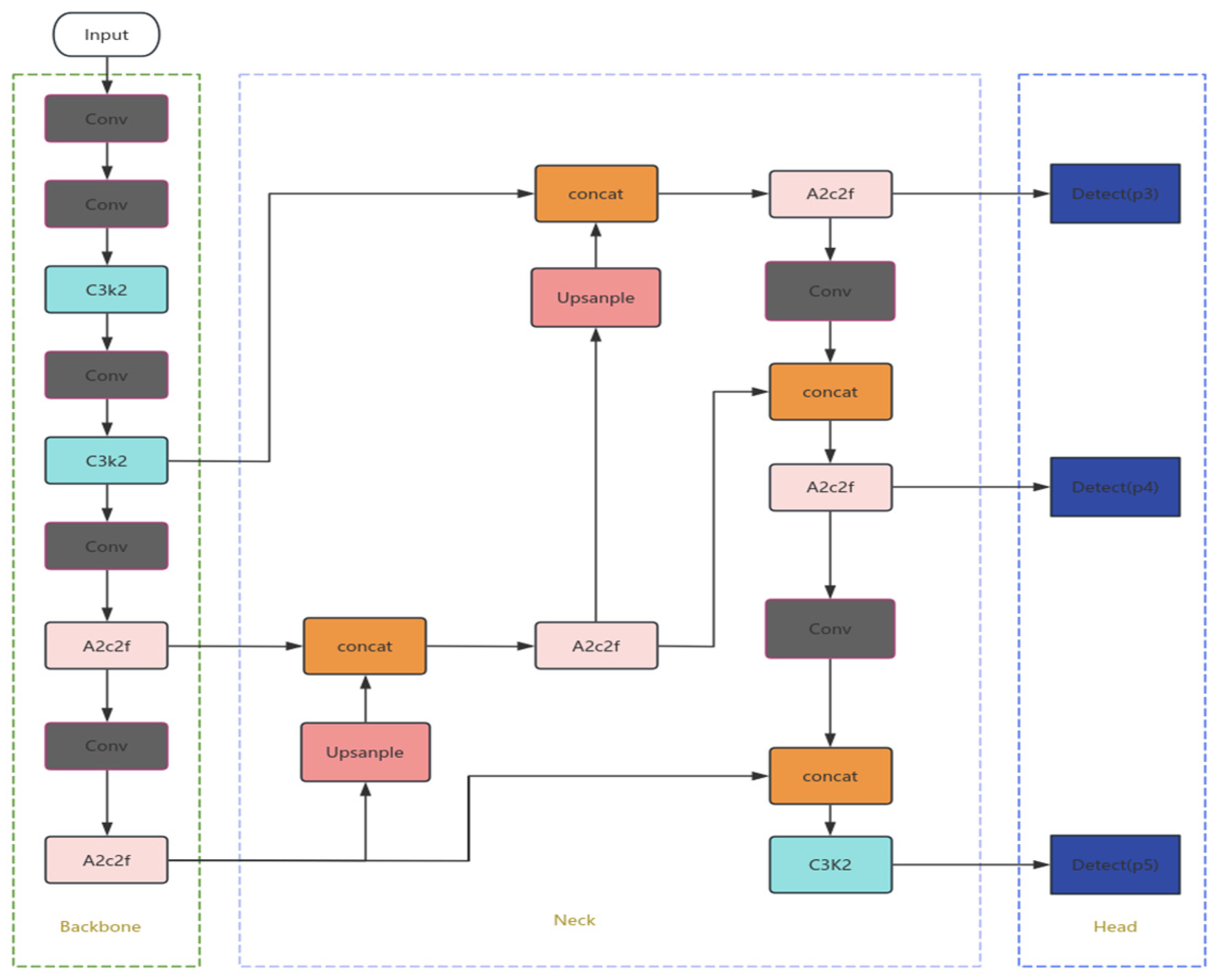
As shown in Figure 1, YOLOv12 follows the typical detector pipeline in which features are first extracted, then fused across scales, and finally converted into prediction outputs. In the feature-extraction stage, convolutional layers and C3k2 residual units generate multi-level representations through successive downsampling [28]. The subsequent fusion stage combines feature pyramid network (FPN) and path aggregation network (PAN) pathways so that shallow spatial details and deeper semantic cues can be integrated across different resolutions. This cross-scale aggregation improves the representation of small targets before the prediction head estimates bounding-box coordinates, category confidence, and objectness. The training objective combines varifocal classification loss with CIoU regression loss to jointly optimize sample classification and localization accuracy.

Currently, YOLOv12 has multiple variants, including n, s, m, i, and x, among which the n and s variants are more suitable for small-target detection. However, due to their ultra-lightweight design, YOLOv12-m and YOLOv12-s exhibit weaker feature extraction capability for thin wires and small pins of transformers, poor anti-interference performance against background noise, and lower regression accuracy for dense pins [29]. Although the base variant retains more network capabilities, it still struggles to capture the features of ultra-small targets, is highly susceptible to interference from metal reflections, and lacks scenario-customized anchor boxes and data augmentation strategies, resulting in insufficient adaptability. Therefore, based on YOLOv12-n, this paper proposes three key improvements in terms of optimizing inference speed, enhancing the attention mechanism, and adjusting the loss function, aiming to design a more adaptive detection algorithm, YOLOv12-Optimized, for industrial components such as small transformers.

2.2.1. RepGhost Reparameterization Technology

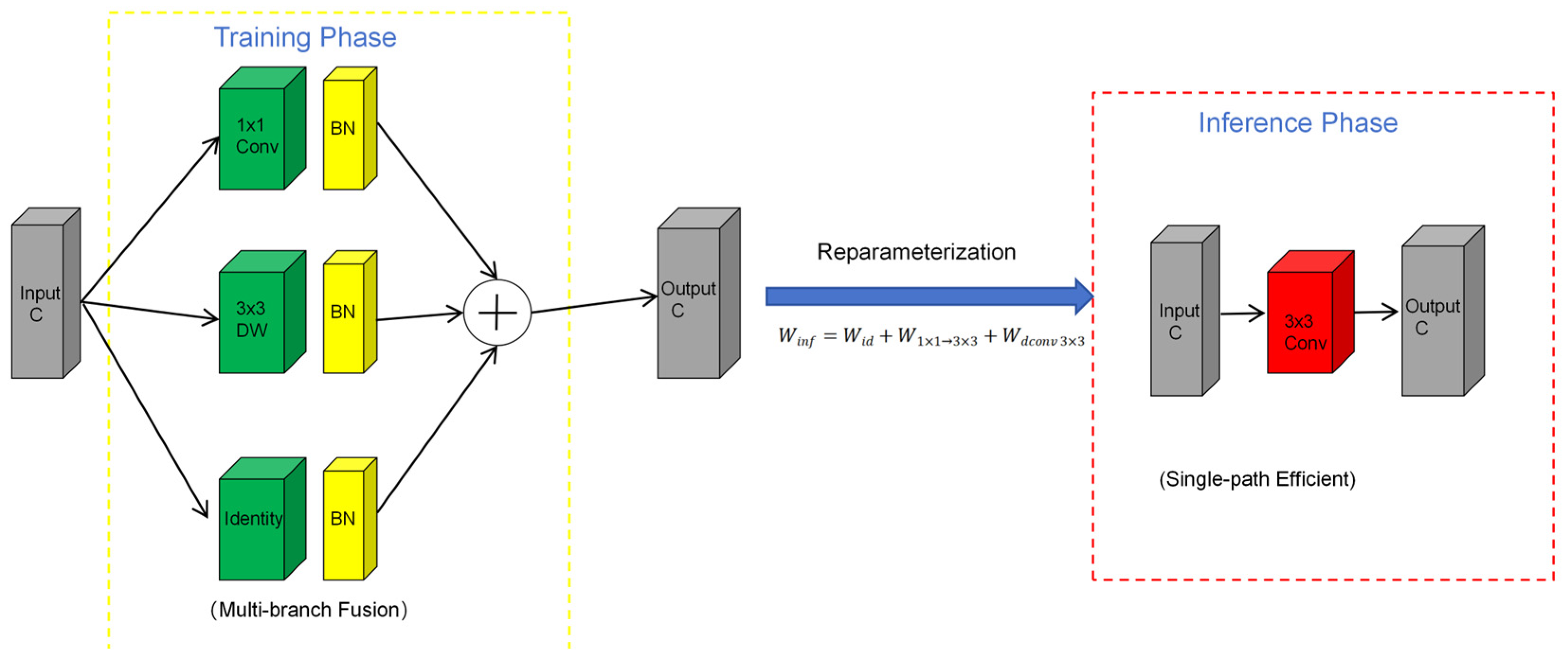
The core of RepGhost is realized through structural reparameterization, which adopts multi-branch enhancement during the training phase and single-path inference during the feature inference phase to improve efficiency. According to the characteristics of the YOLOv12 detection task, the cross-stage partial blocks (CSPBlocks) in the original backbone network are replaced with RepGhost [30]. The specific design is as follows: a multi-branch structure is adopted during training, where each RepGhost consists of 3 parallel branches (the identity branch with batch normalization (BN), the 1 × 1 convolutional branch with BN, and the 3 × 3 depthwise separable convolutional branch with BN). The output feature is the sum of all branches:

$$F_{train}=F_{id}+F_{1\times 1}+F_{dconv 3\times 3},$$

(1)

$$F_{id}=BN\left(F_{in}\right),$$

(2)

$$F_{1\times 1}=BN\left({Conv}_{1\times 1}\left(F_{in}\right)\right),$$

(3)

$$F_{dconv 3\times 3}=BN\left({Conv}_{3\times 3}\left(F_{in}\right)\right),$$

(4)

wherein F_in is the input feature, F_train denotes the output feature of the RepGhost module during the training phase, F_id denotes the output of the identity batch normalization branch, F_1×1 denotes the output of the 1 × 1 convolution branch, and F_dconv 3×3 denotes the output of the 3 × 3 depthwise separable convolution branch. During inference, weight fusion is adopted. Taking advantage of the additivity of linear operators, the weights of multiple branches are fused into a single set of 3 × 3 convolutional weights, achieving cost-free inference. The equation is given as follows:

$$W_{inf}=W_{1\times 1\to 3\times 3}+W_{id}+W_{dconv 3\times 3},$$

(5)

where W_1×1→3×3 denotes the 1 × 1 convolutional weight that is zero-padded to a 3 × 3 kernel size to match the spatial dimension of the depthwise convolution branch, and W_id denotes the equivalent convolutional weight corresponding to the identity mapping branch.

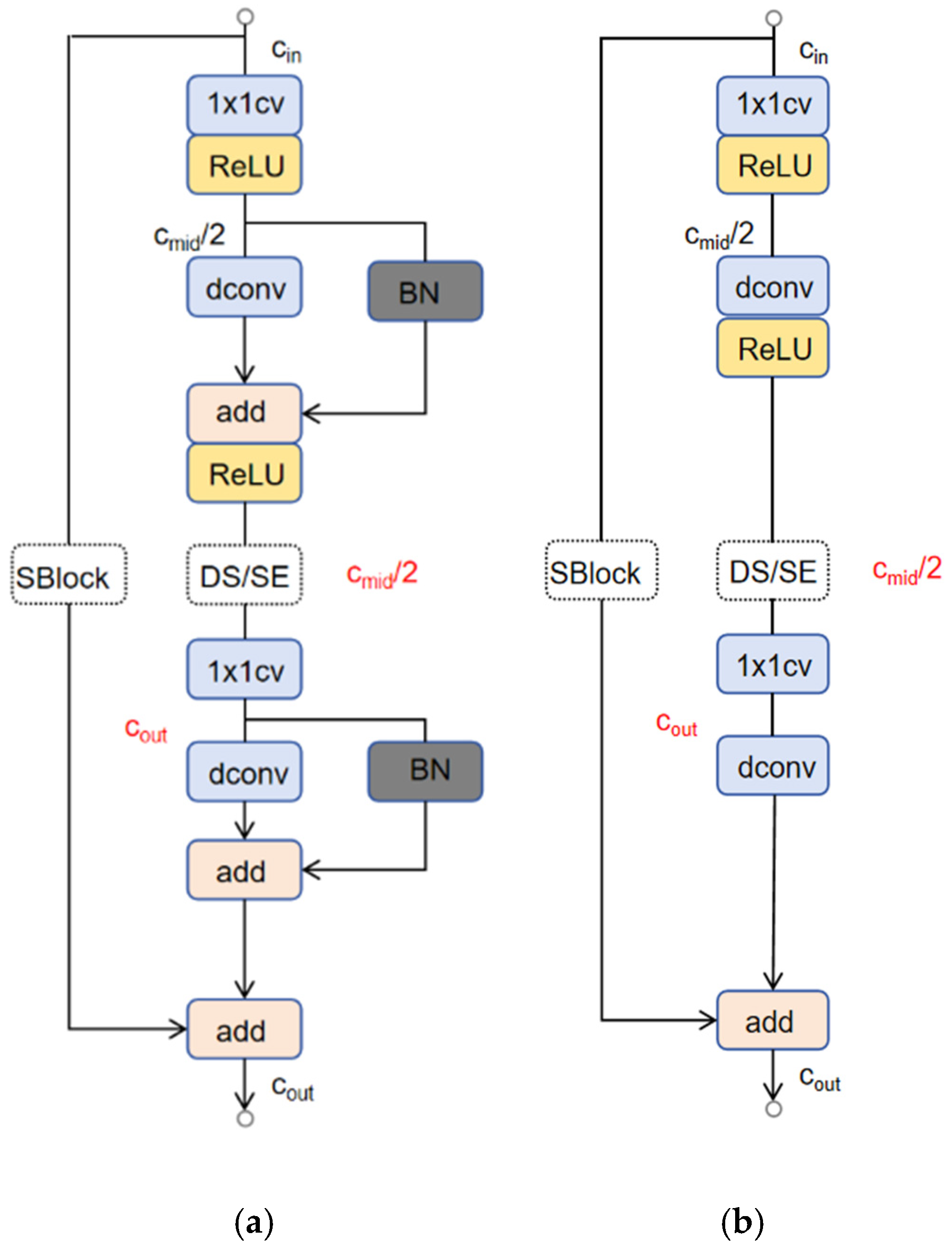
As shown in Figure 2, the RepGhost module first expands the feature channels through the RepGhost 1 feature expansion unit with low-cost operations, then selects the depthwise separable convolution path for feature processing according to the stride (realizing feature map downsampling when stride > 1, and direct transmission when stride = 1), and subsequently embeds an optional squeeze-and-excite (SE) module. This module dynamically calibrates the weights of feature channels through the process of global average pooling, 1 × 1 dimensionality reduction convolution, rectified linear unit (ReLU) activation, 1 × 1 dimensionality elevation convolution, and hard sigmoid activation, thereby enhancing important features such as small transformer damages and suppressing secondary features such as the background. After that, the channel dimension is compressed by the RepGhost 2 feature projection unit, and the features are added together with an optional shortcut connection (residual structure) to finally output the features. This achieves the design goal of multi-branch fusion to enhance feature representation during training and single-branch fusion to improve lightweight efficiency during inference. As shown in Figure 3, the RG-bneck module adopts a multi-branch architecture in the training phase and is converted into a single-path structure through reparameterization during inference.

2.2.2. CBAM Attention Mechanism

The baseline model lacks a feature focusing mechanism for small targets and weak defects, resulting in insufficient attention to important features and high susceptibility to background interference. Although the traditional CBAM attention mechanism can implement channel and spatial attention weighting, it suffers from mismatched receptive fields of spatial attention and imprecise channel weight allocation in small-target scenarios.

Therefore, to address the problem of insufficient small-target feature capture in the original CBAM [31], this paper designs an improved CBAM with pre-enhancement, multi-scale modeling, and residual fusion, which is embedded into the Neck layer of YOLOv12.

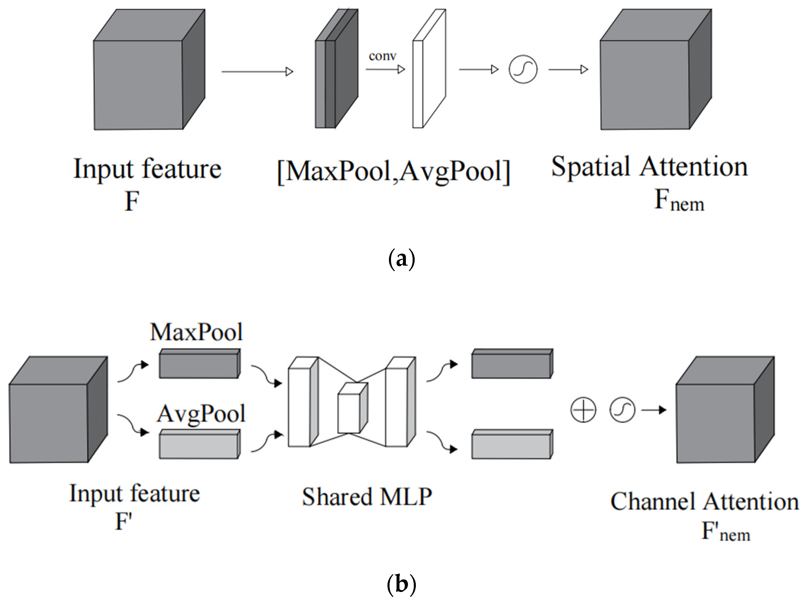
CBAM is composed of two sequential attention units: CAM and SAM. In CAM, global average pooling and max pooling summarize the input features along the spatial dimension, and the resulting descriptors are fed into a shared multi-layer perceptron (MLP) to produce channel-wise weights. After fusion and sigmoid normalization, these weights are used to emphasize informative channels. In SAM, average-pooled and max-pooled feature maps are concatenated along the channel dimension and passed through a convolution layer followed by a sigmoid function, yielding a spatial mask that highlights discriminative locations.

The channel-refined features are further processed by the spatial attention branch, and the resulting attention map is used to recalibrate the original feature representation. By sequentially assigning importance to channels and spatial regions, CAM and SAM help the detector focus on weak defect cues, suppress irrelevant background responses, and improve recognition performance for small transformer defects.

However, as illustrated in Figure 4, the original CBAM attention mechanism exhibits obvious limitations when dealing with ultra-small targets such as pins and wires of small transformers. The feature signals of small targets are weak and prone to being overwhelmed by background factors such as reflections from metal casings. Meanwhile, it only focuses on channel and basic spatial features, failing to fully capture the fine-grained details of small targets. This results in a low recall rate for subtle damages such as wire breakage and missing wires, making it difficult to meet the detection requirements of dense small-target scenarios. To address this issue, the CBAM attention module is improved by adding small-target pre-amplification, multi-scale channel modeling, four-dimensional spatial features, and a residual fusion structure.

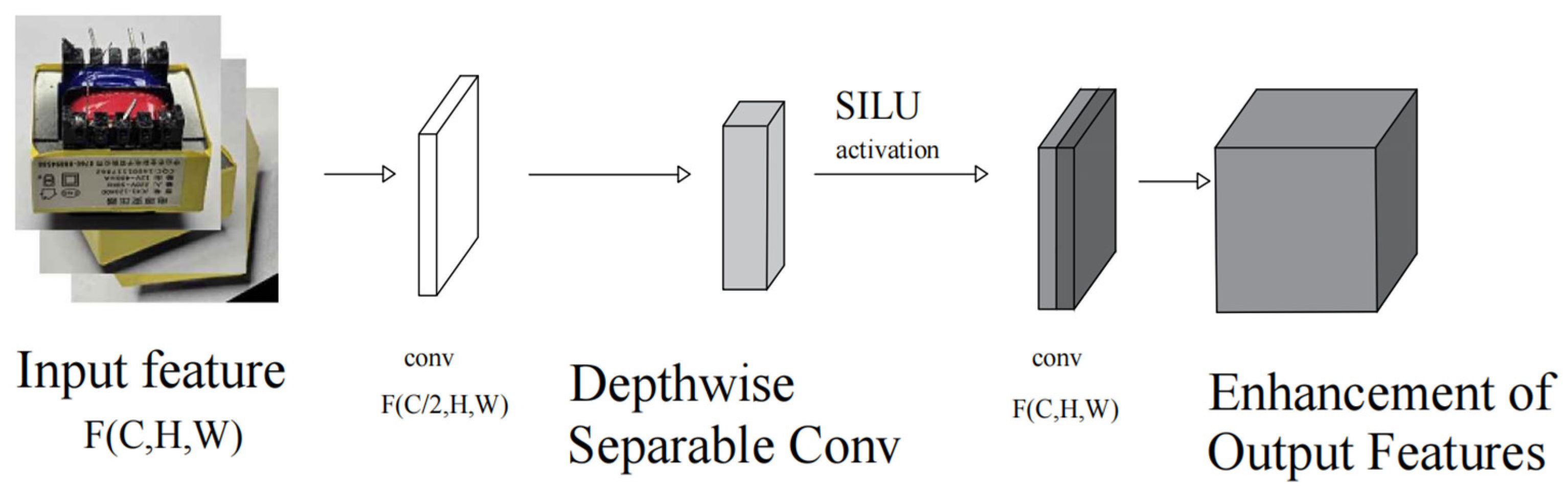
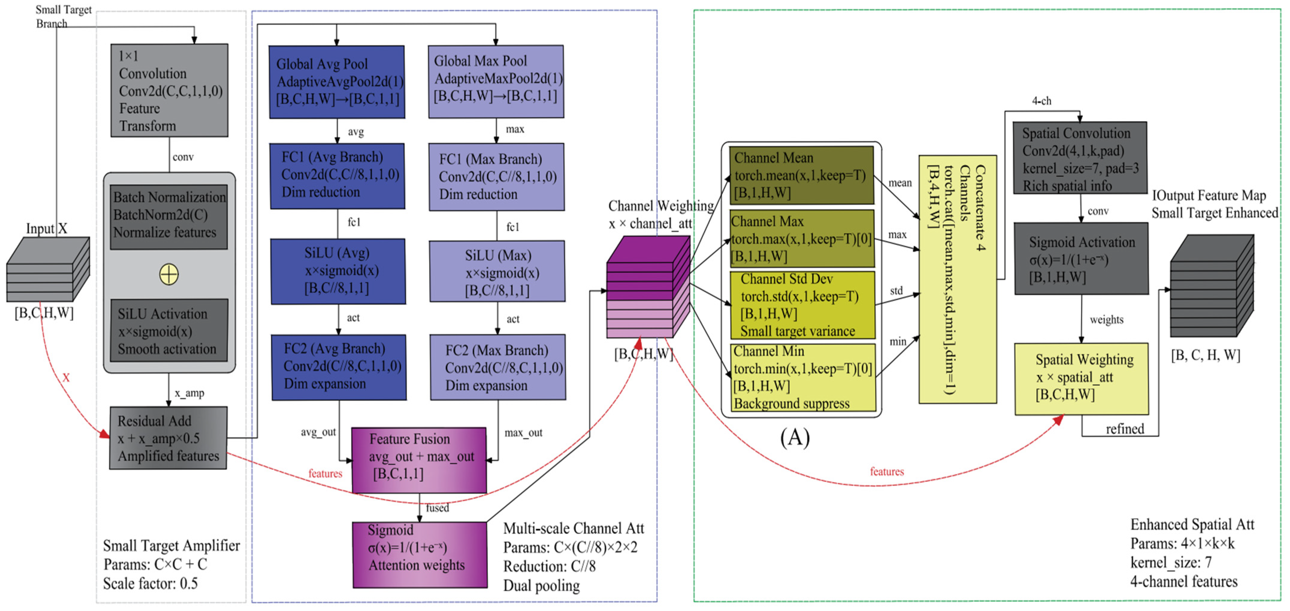
First, on this basis, an additional pre-amplification branch is introduced. Aiming at the pain point of weak feature signals for transformer pins and wires, the pre-amplification branch is designed to generate enhanced features through three-stage operations: channel compression, local feature extraction, and non-linear enhancement, without introducing redundant computations [32]. This provides clear feature inputs for subsequent attention calculation. The structure is as follows:

As shown in Figure 5, the 1 × 1 convolution serves to first compress the number of channels to C/2, reducing the computational complexity of subsequent operations. Meanwhile, it enables information interaction between channels and initially aggregates weak features. A 3 × 3 depthwise separable convolution is employed to replace the standard 3 × 3 convolution, which captures the edge details of pins and wires with almost no additional computational overhead. The sigmoid linear unit (SiLU) activation function is adopted; compared with ReLU, it can better preserve the low-response features of small targets and avoid the truncation of negative weak features by ReLU. Furthermore, its calculation only requires the formula x × sigmoid(x) (where x denotes the feature response value corresponding to each spatial position), which is compatible with the computing power of edge devices.

In the meantime, four-dimensional spatial features are introduced for the fusion of features from multiple statistical metrics. To address the limitation of the original CBAM spatial attention mechanism, which only relies on mean and max values, a four-dimensional feature aggregation module is inserted between the channel attention and spatial attention modules. In terms of the calculation of feature statistics, we adopt the method of processing the output of the channel attention module Fc(H × W × C), calculating four types of statistical metrics along the spatial dimension:

$$F_{avg}\left(c\right)={\displaystyle \frac{1}{H\times W}}{\displaystyle \sum _{i=1}^H}{\displaystyle \sum _{j=1}^W}{F}_c\left(i, j, c\right) ,$$

(6)

$$F_{max}\left(c\right)={}_{i,j}{}^{max}F_c\left(i, j, c\right),$$

(7)

$$F_{min}\left(c\right)={}_{i,j}{}^{min}F_c\left(i, j, c\right),$$

(8)

$$F_{std}\left(c\right)=\sqrt{{\displaystyle \frac{1}{H\times W}}{\displaystyle \sum _{i=1}^H}{{\displaystyle \sum _{j=1}^W}\left(F_c\left(i, j, c\right)-F_{avg}\left(c\right)\right)}^2}.$$

(9)

Thereby generating four 1 × 1 × C feature maps. This is followed by a lightweight fusion and dimensionality reduction process: the four types of feature maps are concatenated into a single 1 × 1 × 4C feature map, which is then compressed to 1 × 1 × C via a 1 × 1 convolution, and finally generated through SiLU activation F_4d(1 × 1 × C) [33].

$$F_{4d}=SILU\left({Conv}_{1\times 1}\left(\left[F_{avg}, F_{max}, F_{std}, F_{min}\right]\right)\right),$$

(10)

where it is combined with spatial attention and F_4d expanded to the dimension of W × H × C. After being concatenated with the original feature map generated by mean and max pooling, a 3 × 3 convolution is applied to generate the spatial attention weights M′_s.

$$M_s^{\prime }=\sigma \left({Conv}_{3\times 3}\left(\begin{array}{c}{F}_{4d}⨂ones\left(H, W, 1\right);\\ avgpool\left(F_c\right);maxpool\left(F_c\right)\end{array}\right)\right),$$

(11)

wherein σ is the sigmoid function. The newly added F_std can distinguish the discreteness of pin edges, F_min. It can capture the dark regions caused by wire loss.

To balance the preservation of small details in images and the detection speed, a residual fusion structure is added. To prevent the loss of small-target details during attention weighting, a residual branch is set at the output end of the improved CBAM, the attention-weighted features F_att and F_amp stack:

$$F_{final}=F_{att}+{Conv}_{1\times 1}^{adapt}\left(F_{amp}\right),$$

(12)

wherein ${Conv}_{1\times 1}^{adapt}$ is an optional channel-adaptive convolution. After superimposition, no additional activation function is applied, and only the feature superimposition operation is added [34].

As shown in Figure 6, unlike vanilla CBAM, which only utilizes global average and maximum pooling, our improved CBAM introduces three task-oriented innovations customized for tiny transformer defects, rather than the simple stacking of existing components. First, a small-target pre-amplification branch based on depthwise separable convolution and SiLU activation is added to enhance faint defect features without extra computation overhead. Second, four-dimensional statistical features (mean, max, min, standard deviation) are fused to capture subtle edge and shadow information of pins and wires. Third, a residual connection is embedded at the output to avoid small-feature suppression caused by attention weighting.

2.2.3. Construction of a Robustness-Enhanced WIoU Loss Function

• Analysis of Loss Functions Related to YOLOv12;

The design of the YOLOv12 loss function continues the core logic of the joint optimization of classification and regression in the YOLO series. It is entirely composed of two components: the varifocal loss (VFL) and the regression loss (including the bounding box regression loss CIoU and the distribution focal loss (DFL)). Through targeted optimizations for the balance between positive and negative samples, focus on hard samples, and bounding box localization accuracy, it adapts to the object detection requirements of complex scenarios with dense small targets and strong background interference. The following analysis will be carried out in combination with the mathematical expressions, parameter meanings, and action mechanisms of the loss functions.

YOLOv12 adopts VFL as its classification loss function, which aims to solve the problems of severe imbalance in the number of positive and negative samples and insufficient classification accuracy for hard samples in object detection [35]. Its mathematical expression is given as follows:

$$VFL\left(p, q\right)=\left\{\begin{array}{c}-q\left[qLnp+\left(1-q\right)Ln\left(1-q\right)\right], q>0\\ -\alpha p^{r}Ln\left(1-q\right), q=0\end{array}\right.,$$

(13)

where q denotes the target quality score, which is defined according to the IoU between the predicted bounding box and its corresponding ground-truth box. The parameter α controls the relative contribution of negative samples in the classification loss. Because background candidates usually far outnumber true defect regions, this coefficient prevents the training process from being dominated by easy negatives. The focusing parameter γ increases the contribution of hard examples, such as small or ambiguous defects. Here, IoU represents the overlap ratio between the predicted and ground-truth boxes, while p denotes the predicted classification confidence. When q > 0, the candidate is treated as a positive sample; when q = 0, it is considered a negative sample.

VFL treats positive and negative samples differently through its piecewise formulation. For positive samples (q > 0), weighted cross-entropy is used, and the IoU-related quality score q serves as the weighting factor [36]. Thus, samples with better localization agreement contribute more strongly to classification optimization, encouraging the classifier to assign higher confidence to accurately localized defects rather than treating all positive anchors equally. For negative samples (q = 0), a focal-style term is applied to down-weight numerous easy background regions while retaining emphasis on confusing background patterns that resemble real defects.

The regression loss of YOLOv12 is designed to optimize the positional deviation between predicted boxes and ground-truth boxes. It is jointly composed of the CIoU loss, which is responsible for the overall localization of bounding boxes, and the DFL, which is dedicated to the detailed regression of bounding boxes [37]. This forms a two-layer regression logic of coarse localization combined with fine-grained optimization.

Wherein, CIoU is an improved version based on the traditional IoU loss. By introducing the center distance penalty and the aspect ratio similarity penalty, it addresses the drawback that the traditional IoU only focuses on the overlapping area while ignoring positional offsets and shape differences [38]. Its mathematical expression is given as follows:

$$L_{CIOU}=1-IOU+{\displaystyle \frac{{\rho }^2\left(b, b^{gt}\right)}{c^2}}+\alpha v,$$

(14)

$$\alpha ={\displaystyle \frac{v}{\left(1-IOU\right)+v}},$$

(15)

$$v={\displaystyle \frac{4}{{\pi }^2}}{\left(arctan{\displaystyle \frac{w^{gt}}{h^{gt}}}-arctan{\displaystyle \frac{w}{h}}\right)}^2.$$

(16)

where α serves as the weight function, and v is used to measure the similarity of the aspect ratios between the predicted boxes and the ground-truth boxes.

Here, w_gt/h_gt and w/h denote the width-to-height ratios of the ground-truth box and the predicted box, respectively. The variables b and b^gt indicate the center coordinates of the predicted and ground-truth boxes. The term ρ measures the Euclidean distance between the two centers, and c is the diagonal length of the smallest enclosing box covering both rectangles.

The other component, DFL, is the loss function employed by YOLOv12 to optimize the details of bounding box regression. Its core objective is to address the adaptation problem where regression targets (such as box coordinates, width, and height) are continuous values, while the model outputs discrete probability distributions. By optimizing the distribution probabilities, it enhances the accuracy of bounding box regression. Its mathematical expression is given as follows:

$$DFL\left(S_i, S_{i+1}\right)=-\left[\left(y_{i+1}-y\right)Ln\left(S_i\right)+\left(y-y_i\right)Ln\left(S_{i+1}\right)\right],$$

(17)

as shown in Equation (17), S_i and S_i+1 denote the predicted distribution probability value, representing the model’s prediction confidence that the target regression boundary (e.g., coordinates, width, height, etc.) falls within the discrete interval [i, i + 1]. It is the output of the predicted distribution in DFL. y_i is the label value of the discrete interval, and y is the true continuous regression target value (e.g., continuous values such as the coordinates and dimensions of the ground-truth box).

The essence of DFL is to enable the model to learn the precise position of the continuous regression target by optimizing the probability distribution of discrete intervals. For the interval [i, i + 1] where the true value y lies, DFL uses the weights of (y_i+1–y) and (y–y_i) to make the model prioritize increasing the probability of the interval endpoints close to y (e.g., when y is close to i + 1, (y_i+1–y) is decreased, (y–y_i) is increased, which guides the probability of S_i+1 to rise).

This distribution-based learning approach can effectively alleviate the class imbalance problem in regression tasks, such as the scarcity of samples in certain intervals. Meanwhile, it enhances the model’s sensitivity to deviations of small-scale bounding boxes. For instance, when YOLOv12 detects small targets (e.g., pins), DFL enables the model to accurately capture bounding box offsets at the 1 mm level, thereby avoiding missed detections or false detections caused by regression errors.

The core improvement of CIoU over the traditional IoU lies in the fact that it not only requires a high overlap between the predicted box and the ground-truth box, but also mandates center alignment and shape similarity, which improves the bounding box localization accuracy. However, CIoU still has certain limitations. First, its calculation involves the arctan inverse trigonometric function, which increases the computational cost of the model and especially affects the inference speed in large-scale object detection tasks. Second, it fails to consider the loss balance between low-quality predicted boxes and high-quality predicted boxes, adopting a unified penalty logic for all samples. Third, the term v only focuses on the degree of difference in aspect ratios. When the predicted box and the ground-truth box have the same aspect ratio but a large difference in size, it cannot reflect the actual localization deviation.

• Application and Improvement of WIoU.

Compared with the current limitations of CIoU, the adaptive advantages of WIoU over CIoU for transformer quality inspection are manifested in the following three aspects: Firstly, it is more lightweight and efficient, as CIoU involves the arctan inverse trigonometric function leading to high computational cost, while WIoU removes this operation to achieve a significant reduction in computation time, making it better suited for real-time detection on edge devices and thus aligning with the real-time requirements of small transformer production lines; secondly, it enables more accurate optimization for small targets, for CIoU is prone to penalty loss for small targets such as transformer pins and wires when there is size scaling without changes in aspect ratio, while WIoU normalizes the center distance by the size of the ground-truth box, which can amplify the loss even for offsets at the 1 mm level and thereby improve the recall rate of small targets; thirdly, it has stronger robustness against annotation errors, since the dense distribution of transformer pins makes them highly susceptible to misannotation and CIoU is sensitive to such errors, whereas the dynamic weight mechanism of WIoU can reduce the interference of abnormal annotation gradients.

Meanwhile, the adaptive advantages of WIoU over other loss functions (distance intersection over union (DIoU), efficient intersection over union (EIoU)) are as follows: DIoU only optimizes the center distance and cannot correct the slender shape deviations of transformer wires, while although WIoU does not have a separate aspect ratio term, it indirectly improves shape adaptability by dynamically focusing on samples of ordinary quality; EIoU imposes excessive penalties on small targets, leading to training oscillations, whereas WIoU adopts gentle size normalization, which reduces the proportion of loss caused by small-target deviations, makes the model training more stable, and meets the lightweight requirements [39].

Currently, there are three versions of WIoU, among which WIoUv1 constructs an attention-based bounding box loss, while WIoUv2 and WIoUv3 add a focusing mechanism on this basis by designing a calculation method for gradient gain (focus coefficient). The calculation of the WIoUv1 loss function is given as follows:

$$L_{IOU}=1-IOU,$$

(18)

$$R_{WIOU}=exp\left({\displaystyle \frac{{\left(x-x_{gt}\right)}^2+{\left(y-y_{gt}\right)}^2}{\left(W_g^2+H_g^2\right)}}\right),$$

(19)

$$L_{WIOU v1}=R_{WIOU}{L}_{IOU},$$

(20)

$$L_{WIOU v2}={\left({\displaystyle \frac{L_{IOU}^{*}}{\overline{L_{IOU}}}}\right)}^{\gamma }{L}_{WIOU v1}.$$

(21)

where L_IoU denotes the non-overlap degree between the predicted box and the ground-truth box, and IoU is defined as the ratio between their intersection area and union area. R_WIoU represents the penalty coefficient used to describe the relative center-distance deviation. The variables x and y denote the center coordinates of the predicted box, whereas x_gt and y_gt denote those of the ground-truth box. W_g and H_g are the width and height of the minimum enclosing rectangle covering both boxes. In Equation (21), the normalized L_IoU term acts as a monotonic focusing coefficient.

$$\beta ={\displaystyle \frac{L_{IOU}^{*}}{\overline{L_{IOU}}}}\in \left[0,+\infty \right),$$

(22)

$$L_{WIOU v3}=\gamma L_{WIOU v1}, \gamma ={\displaystyle \frac{\beta }{\delta {\alpha }^{\beta -\delta }}}.$$

(23)

As shown in Equations (22) and (23), β is the non-monotonic focusing coefficient; α and δ are hyperparameters; γ is the gradient gain.

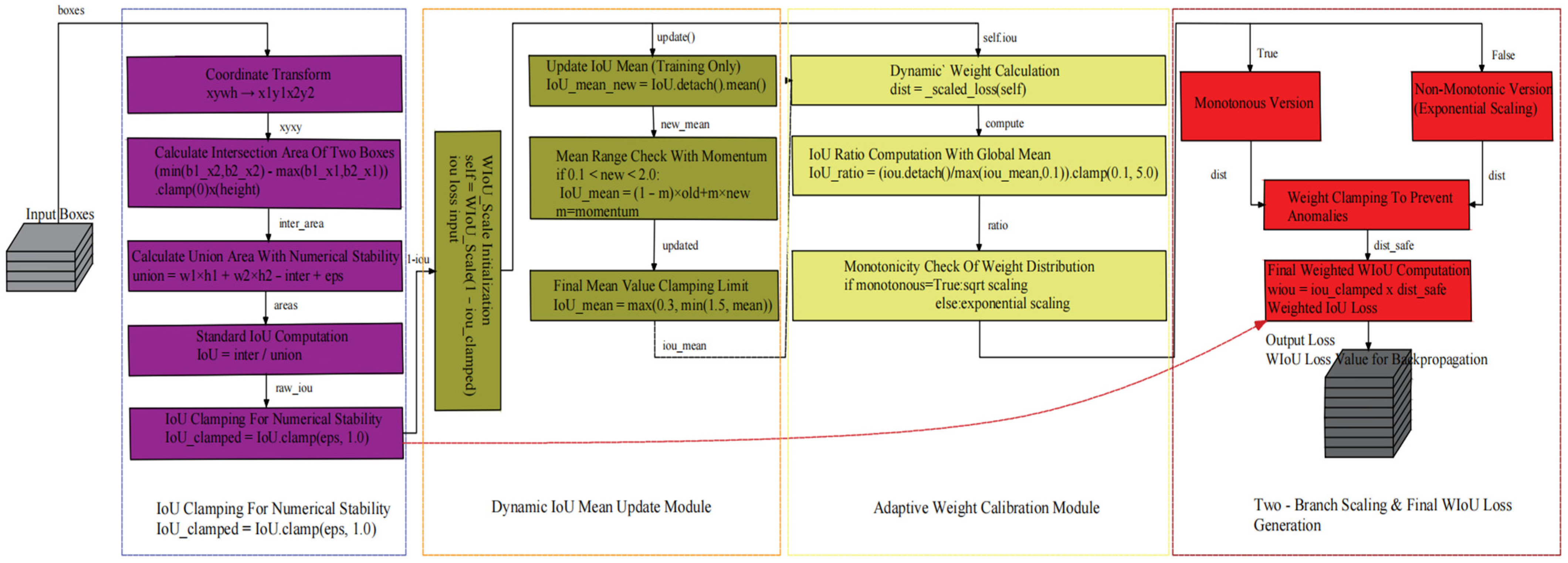
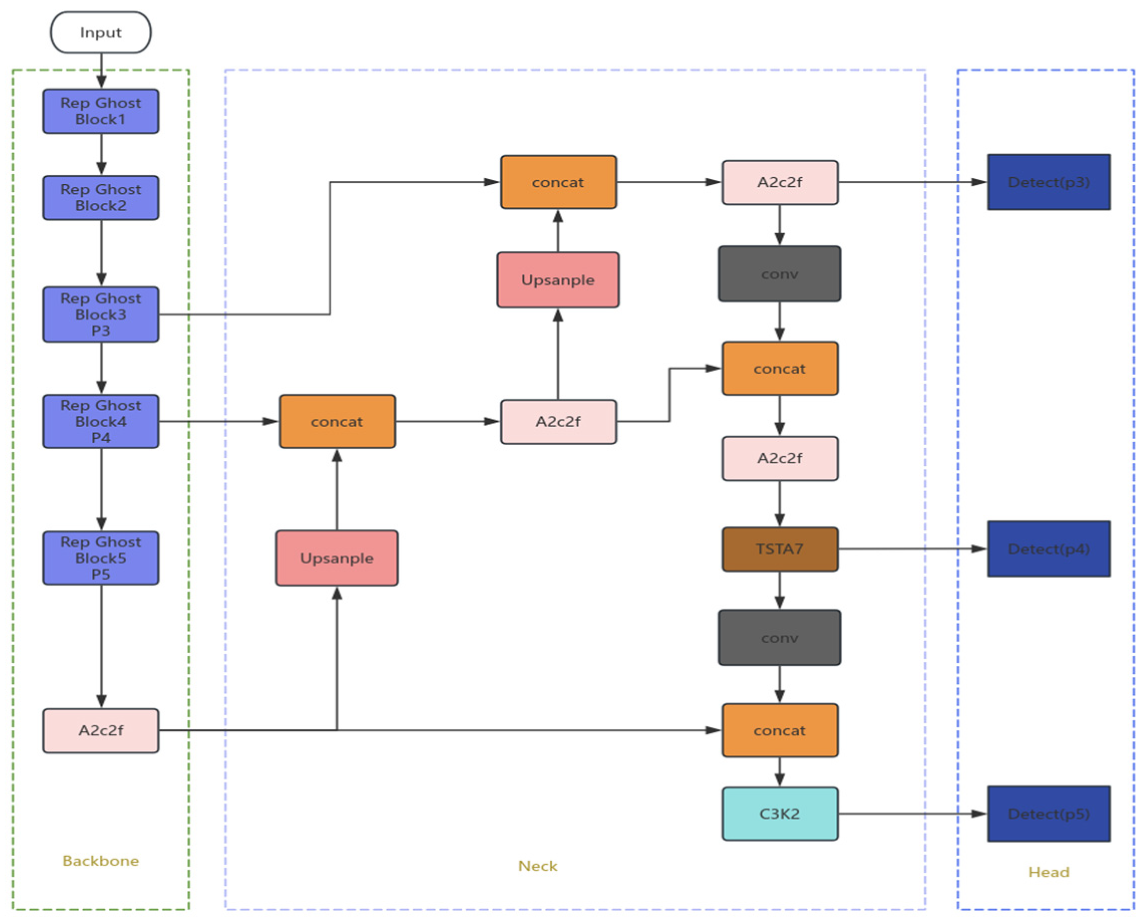
As shown in Figure 7, the proposed WIoU loss contains multiple optimization modules. Compared with the original WIoU series loss, two novel constraint mechanisms are proposed to tackle dense pin annotation noise in industrial scenes. A dual numerical clamping mechanism limits the range of IoU and gradient values to prevent training oscillation. A momentum weight restriction module adaptively adjusts sample loss weights according to training epochs, weakening the negative impact of inaccurate manual labels. As shown in Figure 8, the improved YOLOv12 network consists of three components: the Backbone, the Neck, and the Detection Head.

3. Experimental Setup and Evaluation Metrics

3.1. Data Source

3.1.1. Transformer Sample Collection and Artificial Defect Fabrication

The detection object of this paper is the small low-frequency power transformer JC41-120400 (Zhongshan Jincai Electronics Co., Ltd., Zhongshan, China), which is widely used in consumer electronic chargers, switching power supplies and household electrical control modules. Over 30 defective transformers of the same model with faults generated during production were collected to serve as references for image acquisition and artificial defect simulation. In addition, several finished transformers were used to fabricate artificial defects, and 3539 original RGB images were captured under a fixed industrial inspection lighting environment. During image acquisition, three mandatory shooting perspectives shall be captured for each identical sample: front view, 45° top-left view and 45° top-right view. These three angles match the single-station camera layout of online inspection equipment deployed in actual manufacturing factories. In addition, transformers may shift or rotate to varying degrees while being conveyed on production belts during real-world production. For this reason, several extra shooting angles are incorporated into the image-capturing workflow to boost detection accuracy.

To construct a complete defect dataset covering common production failure modes, we first statistically analyze the defect features generated during factory manufacturing. The core statistical indicators include the proportion of different defect types and the severity distribution within each defect type. Subsequently, a manual dataset is fabricated to expand the training data volume. All defective samples in this paper are manually produced with professional maintenance tools, and detailed standardized operating procedures are adopted for each defect category to introduce sufficient morphological variations, multi-level severity grades, and composite defect combinations. The specific fabrication scheme for each defect type is described as follows:

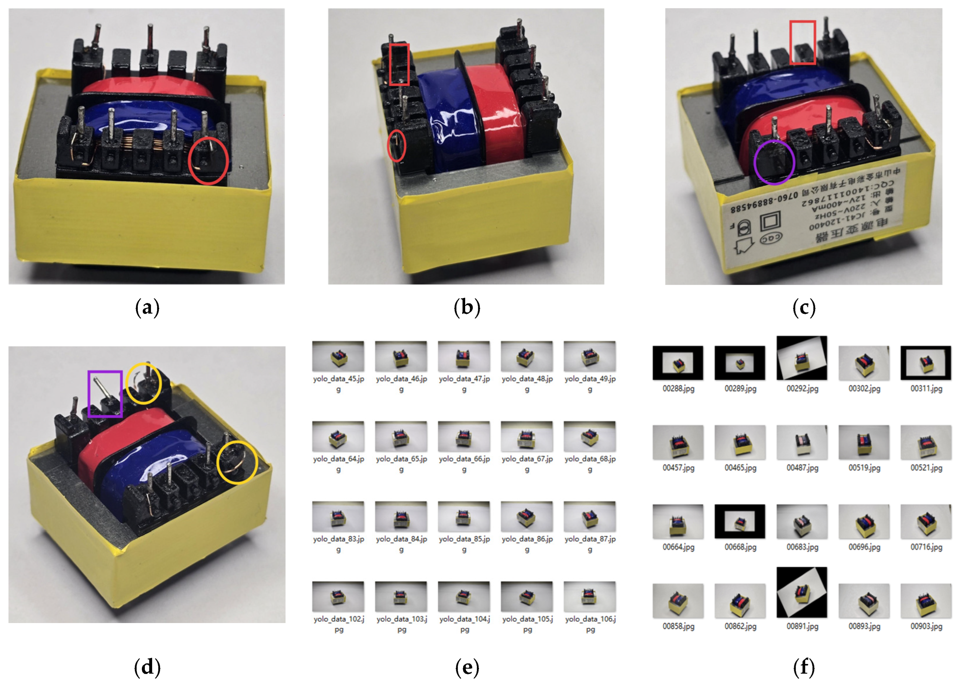
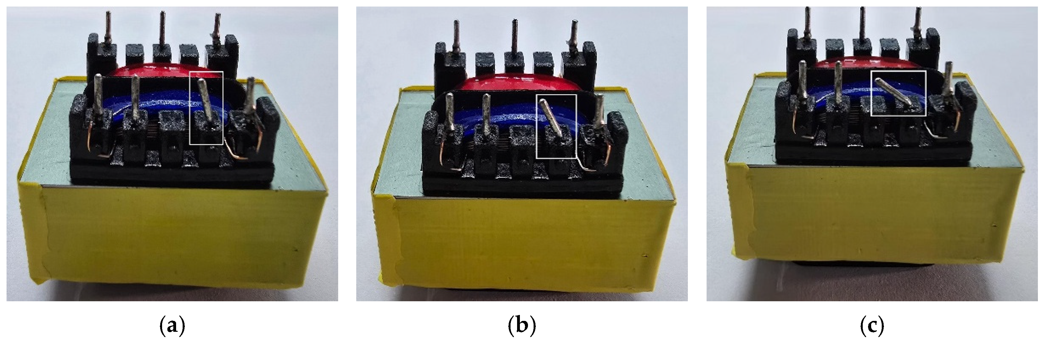
• Bent pins: Tweezers are used to apply controlled bending deformation to the metal pins of transformers. The bending directions are set with reference to actual pin defects occurring during industrial production. The vast majority of pin-bending defects generated in routine production stem from extrusion during assembly and transportation, which causes pin deformation. Drawing on real sample data, the bending angle range is set from 5° to 45°. Three severity levels are classified based on the pin offset ratio: slight bending (5–15°), moderate bending (16–30°), and severe bending (31–45°), as shown in Figure 9.
• Missing pins: At present, most small and medium-sized enterprises adopt semi-mechanical processing for pin assembly. First, machines insert copper pin wires into pre-reserved holes, followed by a cutting process. As a result, pin missing defects frequently occur in production due to improperly reserved hole positions or failure to replenish copper wires in a timely manner after depletion. Statistical real-world data indicate that pin missing defects have no severity grading and are simply categorized into two states: pin present and pin absent. During manual defect fabrication, pliers are used to pull out target pins to simulate the scenario where pins fail to be inserted. To replicate pin loss caused by missing pre-drilled holes, pliers are employed to extract pins, and black filler is applied to fill the vacant holes.
• Wire breakage, missing wires: Incomplete wire soldering and excessively short reserved length of coil winding wires are both causes of wire defects that lead to wire breakage. Wires that fail to protrude or have an overly short exposed segment result in missing wires. A distinction is made between these two conditions as different remedial measures are required for each. Scissors are used to trim the wires during sample preparation: wires with an exposed length less than 5 mm are classified as missing wires, while those with an exposed length exceeding 5 mm are categorized as broken wires. The damages in the dataset are shown in Figure 10.

In terms of multi-defect sample configuration, statistics from more than 30 groups of real factory samples show that approximately 28% of images contain two or more simultaneous defects, which aligns with real industrial scenarios where multiple faults may occur on a single component at the same time. Typical combined defects include bent pins plus broken wires, missing pins plus missing wires, and bent pins plus missing wires. For multi-defect images, each independent defect region is labeled with a separate bounding box, enabling the model to learn to detect all coexisting defects simultaneously. Meanwhile, to boost the detection accuracy of transformers with multiple defects, around 70% of samples were manually configured to contain multiple defects during dataset construction, so as to improve the detection precision for cases with concurrent defects.

Simultaneously, it is necessary to clarify the inherent limitations of the manually fabricated defect dataset. The artificially manufactured defects have regular, standardized deformation and damage morphology, while real defects generated on the production line have random, irregular shapes. In addition, real industrial transformers are often accompanied by interference factors such as surface oil stains, metal oxidation, plastic dust and accidental extrusion deformation, which are not fully reproduced in our current laboratory acquisition environment. Therefore, the dataset in this paper is suitable for algorithm verification and prototype performance testing under controlled laboratory conditions; future research will collaborate with transformer manufacturers to extensively collect unprocessed, real defective products from production lines for further model validation and transfer learning optimization.

3.1.2. Dataset Class Distribution and Intra-Class Sampling Strategy

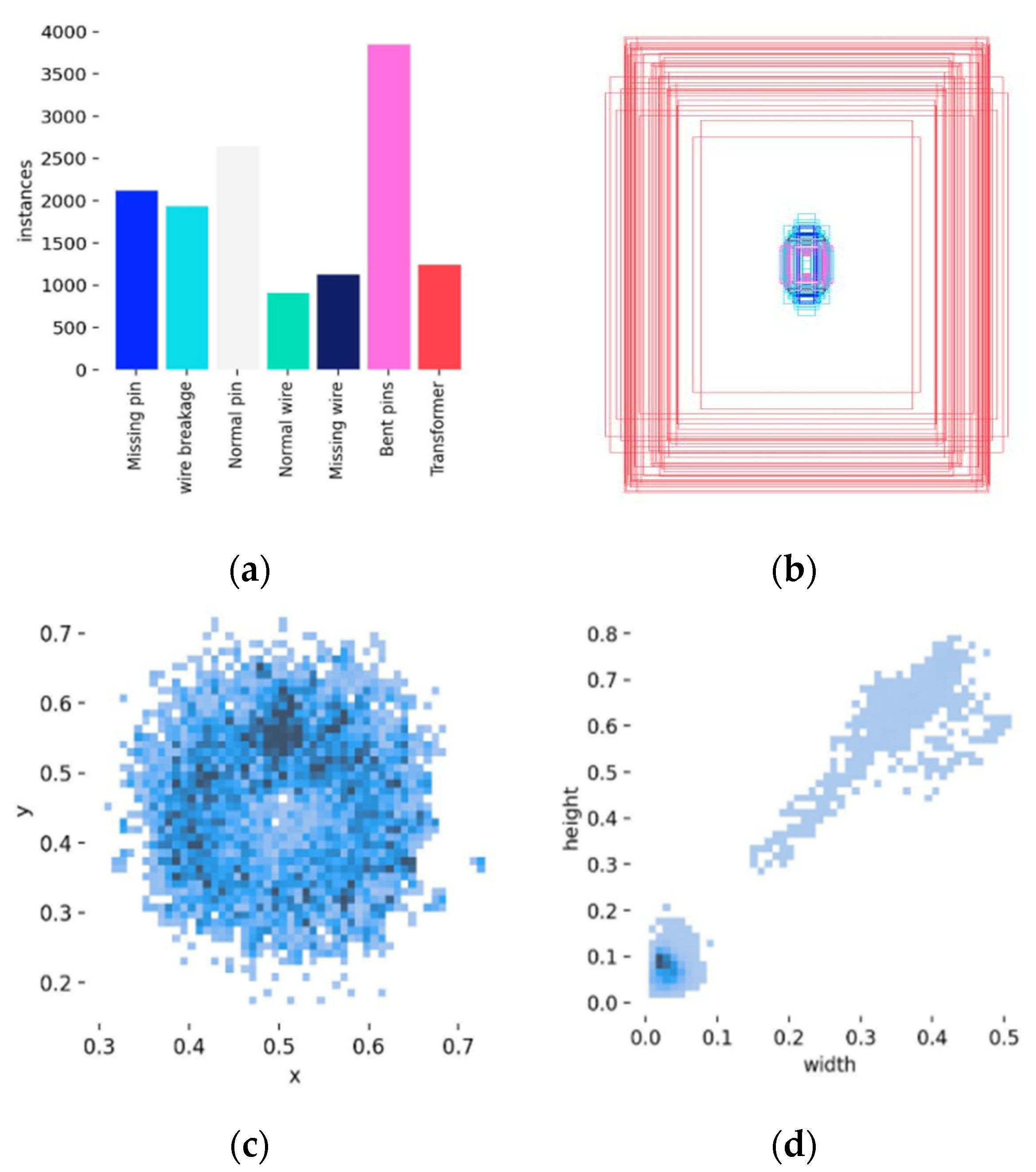
The dataset contains one global object category (transformer) and six fine-grained defect categories (normal pins, bent pins, missing pins, wire breakage, missing wire, normal wire). The number of samples for each category is unbalanced, and the sampling imbalance is designed based on two industrial practical factors:

• Actual on-site defect occurrence frequency: Bent pins and wire breakage are the two most frequent faults in transformer assembly and winding processes, so we allocate more sampling quantities for these two categories to make the training distribution consistent with real inspection data distribution. Missing pins and missing wires belong to low-probability assembly failures; thus, corresponding sample quantities are appropriately reduced.
• Intra-class geometric variability: Pin-related defects have abundant variable dimensions, including pin position, bending direction and bending severity, requiring a large number of samples to cover the complete feature space. In contrast, missing pins have a single fixed morphological feature, so that fewer samples can complete feature learning.

3.1.3. Class Definition and Standard Annotation Protocol

All images are annotated with LabelImg open-source annotation software, following fixed dual-layer annotation specifications:

• Step 1: Draw one independent outer bounding box for the whole transformer component in every image, marked with the label “Transformer”. The category labeled “Transformer” represents the complete main body of the small transformer component, regardless of whether the surface contains defects or not. This global localization label is designed as the primary detection target of the model: the network first locates the overall transformer region from the complex background image, and then extracts local features inside the transformer bounding box for fine-grained defect detection, which eliminates the interference of irrelevant background pixels and improves small defect feature extraction efficiency. Both defect-free intact transformers and defective transformers are annotated with the transformer bounding box.
• Step 2: For images containing any surface defects, draw an independent small bounding box for each visible defect area inside the transformer box, and mark the corresponding defect category label (bent pins/missing pins/wire breakage/missing wire). Meanwhile, small bounding boxes also need to be drawn separately for intact normal pins and wires, labeled as “Normal Pin” and “Normal Wire”, respectively.

As a result, one defective image contains 1 global transformer label plus multiple independent defect labels. All evaluation metrics are calculated based on all annotated categories synchronously, which can comprehensively evaluate both the overall component localization ability and the tiny defect fine-grained detection performance of the model.

3.1.4. Dataset Partitioning Strategy and Anti-Leakage Design

To truly evaluate the model’s generalization ability to unseen brand-new transformers and avoid data leakage caused by multi-view images of the same physical component, this paper adopts “device-level independent partitioning logic” instead of random image-level splitting. Subsequently, the original dataset is split into training, validation and test subsets following a 6:3:1 partition ratio.

Core partitioning constraint: All multi-view shot images of one identical physical transformer are assigned to only one subset. Images of the same component will never simultaneously appear in the training set and test/validation sets. This scheme ensures that all transformer entities in the test set are completely unseen samples for the model, and the test mAP results can objectively reflect the model’s generalization performance on new offline inspection components, eliminating the overestimated performance caused by repeated device pictures across different subsets, the classification and labeling status of the dataset are shown in Figure 11.

3.1.5. Data Augmentation Implementation Details and Execution Timing

Data augmentation is applied only to the training subset after dataset partitioning, and no augmentation operation is executed on validation and test images, which thoroughly avoids data leakage where transformed copies of one original image exist in multiple subsets and inflate detection accuracy. All augmentation operations are online random transformations executed during each training epoch, and all image augmentation functions are implemented based on the OpenCV 4.8.0 and Albumentations 1.3.1 Python libraries within the PyTorch training framework.

The complete augmentation strategies, corresponding execution probability and parameter range are listed as follows:

• Random horizontal flip, execution probability = 0.5;
• Random rotation within the range of −15°~+15°, execution probability = 0.4;
• Random brightness and contrast adjustment with ±20% variation range, execution probability = 0.3;
• Mosaic 4-image hybrid splicing augmentation, execution probability = 0.3;
• Random scaling and cropping, scaling range 0.8–1.2 times the original image size, execution probability = 0.3.

The original training set contains 2123 static images. After online random augmentation in each training cycle, the equivalent effective sample volume per epoch expands to approximately 7400 diversified samples, which effectively suppresses model overfitting on limited industrial defect data and improves the robustness of the model to different lighting, angles and component placement positions.

3.1.6. Defect Visibility, Viewpoint Constraints and Occlusion Discussion

The image acquisition system captures three fixed perspectives (front, 45° left, and 45° right) as well as other auxiliary viewing angles for each transformer. Under these shooting perspectives, there are significant differences in the visibility of various defect categories:

• Pin-type defects (normal pin, bent pins, missing pins) are distributed on the top flat plastic base of the transformer. Under the front-top shooting angle, all pin areas are completely exposed to the camera’s field of view, with almost no natural occlusion.
• Linear defects (wire breakage, missing wires) are distributed on the side winding framework of transformers. The combination of the three mandatory shooting perspectives (front, 45° left, and 45° right) and auxiliary perspectives can fully cover the front winding lead areas where most wire defects occur.

In addition, transformers may shift during actual inspection, making it difficult for the three fixed perspectives to accurately capture the front, 45° left, and 45° right views of the transformer. To avoid this issue in practical applications, video recording is integrated into the image capture system. Frames are extracted from the recorded video to generate auxiliary perspectives. Combined with the three fixed shooting angles, this setup can cover nearly all images required for inspecting the four wires on both sides.

3.2. Experimental Configurations and Evaluation Metrics

To ensure the training stability of the appearance defect detection model for small transformers, the reliability of data collection, and the effectiveness of system joint debugging, this experiment constructs a complete experimental system from three dimensions: hardware selection, software adaptation, and metric design. All configurations are customized for the core characteristics of dense small targets, difficult identification of weak defects, and high real-time performance requirements, ensuring that the experimental results are reproducible and verifiable.

3.2.1. Hardware Environment Configuration

The experimental hardware system is divided into four major modules: computing hardware, image acquisition hardware, data transmission and power supply hardware, and fixed support hardware. All modules are collaboratively adapted to the requirements of laboratory and industrial quality inspection scenarios, ensuring the accuracy of data acquisition and the efficiency of model operation. The computing hardware adopts the Lenovo Legion Y9000X (Lenovo Group Ltd., Beijing, China), a mainstream choice for current consumer-grade and laboratory scenarios. It balances computing performance and cost-effectiveness, and can stably support the full-process training and real-time inference of deep learning models. Its central processing unit–graphics processing unit (CPU-GPU) combination can satisfy multiple rounds of model iteration without performance degradation. The 32 GB high-frequency memory and high-speed non-volatile memory express solid-state drive (NVMe SSD) ensure the read/write speed of large-scale datasets and the iteration efficiency of model parameters. The core of the image acquisition system selects the Hikvision MV-CA060-10GC color industrial camera (Hangzhou Hikvision Digital Technology Co., Ltd., Hangzhou, China). With 6 million effective pixels, it can achieve an imaging accuracy of ≤0.01 mm actual size per pixel. Combined with a ring-shaped uniform light source and a high-precision fine-tuning bracket, it effectively solves the imaging challenges in industrial scenarios such as reflections on metal pins and occlusion of small-target defects. Gigabit Ethernet is adopted for data transmission, with a single-frame transmission time of ≤50 ms, which meets the frame rate requirements under real-time detection mode. A 12 V stable power supply module ensures long-term operation of the equipment without interference from voltage fluctuations. The specific hardware configuration parameters are shown in

Table 1. Hardware configuration parameters.

Equipment Category	Equipment Name	Specific Configuration Parameters
Computing Hardware	Lenovo Legion Y9000X	CPU: Intel Core i5-14600KF GPU: NVIDIA GeForce RTX 4060 Memory: 32 GB DDR5 5600 MHz Storage: 1 TB NVMe SSD
Image Acquisition Hardware	Industrial Vision Kit	Camera: Hikvision MV-CA060-10GC Color Industrial CameraLight Source: Ring Uniform Light SourceLens: 12 mm Fixed Focal Length Lens
Data Transmission & Power Supply	Auxiliary Hardware	Transmission: Gigabit Ethernet CablePower Supply: 12V/5A Stable Power Supply ModuleControl: Camera IO Trigger Signal Cable
Fixed Support Equipment	Positioning Bracket	High-precision Fine-tuning Vision Bracket Supporting X/Y/Z 3-axis Adjustment

.

3.2.2. Software Environment Configuration

The software environment is constructed around a three-layer architecture comprising hardware drivers, algorithm development, and interface joint debugging, which ensures the coordinated and stable operation of all modules while adapting to the practicality and scalability requirements of industrial scenarios. The Windows 11 Professional operating system is designed to guarantee hardware driver compatibility and software runtime stability. The deep learning framework employs PyTorch 2.1.0 paired with Compute Unified Device Architecture (CUDA) 12.1, providing efficient computing power support for model training. The core development libraries include Python 3.9.18, OpenCV 4.8.0, and others, which meet the requirements of image preprocessing, model inference, and visualization. LabelImg 1.8.6 is used for data annotation, following the pascal visual object classes (VOC) format to ensure annotation accuracy. The Hikvision camera software development kit (SDK) V4.2.0 is selected as the hardware driver to achieve seamless communication between the industrial camera and the software system. The specific software configuration parameters are shown in

Table 2. Software configuration parameters.

Software Category	Tool Name	Specific Configuration Parameters
System Platform	Operating System	Windows 11 Professional Edition
Deep Learning Framework	Core Framework	PyTorch 2.1.0, CUDA 12.1, CuDNN 8.9.2
Core Development Library	Development Toolkit	Python 3.9.18, OpenCV 4.8.0, NumPy 1.26.0, Matplotlib 3.7.1, PyQt5 5.15.9
Data Annotation & Management	Annotation & Storage Tools	labelImg 1.8.6, SQLite 3.41.2
Hardware Driver & Tools	Driver & Debugging Tools	Hikvision Camera SDK V4.2.0, MVS 4.2.0 Machine Vision Client
Auxiliary Development Tools	Prototype Verification Tools	Halcon 20.11, VisionPro 10.0

.

3.2.3. Design of Evaluation Metrics

In combination with the industrial requirements of dense small targets, difficult identification of weak defects, and high real-time performance for appearance defect detection of small transformers, this paper adopts loss function curves, mean average precision (mAP@0.5), precision, recall, F1-score, frames per second (FPS), params, and floating point operations (GFLOPs) as core evaluation metrics to comprehensively quantify the detection performance, real-time performance, and lightweight level of the model.

Precision refers to the ratio of the number of correctly predicted defective samples to the total number of samples predicted as defective, which is used to measure the model’s ability to suppress false detections. Its calculation formula is shown in Equation (24).

$$P={\displaystyle \frac{TP}{TP+FP}},$$

(24)

wherein true positive (TP) denotes the number of correctly detected defective samples of small transformers, and false positive (FP) denotes the number of samples where normal components or background are misclassified as defective.

Recall refers to the ratio of correctly predicted defective samples to the total number of actual defective samples, which is used to measure the model’s ability to suppress missed detections (e.g., omissions of pin breakage and wire loss). Its calculation formula is shown in Equation (25).

$$R={\displaystyle \frac{TP}{TP+FN}},$$

(25)

wherein false negative (FN) denotes the number of actual defective samples that are not detected.

Mean average precision (mAP@0.5) is used as the core evaluation metric to comprehensively measure the model’s detection accuracy for various types of defects. First, the average precision (AP) for each defect category is calculated from the precision-recall (PR) curve, where AP refers to the integral area under the PR curve. Then, the arithmetic mean of APs across all defect categories is computed to obtain mAP@0.5 (with the IoU threshold fixed at 0.5 to meet the bounding box matching requirements of industrial quality inspection). Its calculation formula is shown in Equation (26).

$$mAP@0.5={\displaystyle \frac{1}{c}}{\displaystyle \sum _{k=1}^c}\left(A{P}_k\right),$$

(26)

where C denotes the total number of annotated detection categories in the small-transformer dataset (C = 7 in this study), and AP_k represents the average precision of the k-th category.

The loss function curves include the bounding box loss curve and the classification loss curve, which are used to reflect the convergence during model training. A curve that decreases smoothly and stabilizes eventually indicates that the model training is effective, without gradient oscillation or non-convergence issues. FPS refers to the average inference frame rate for a single 640 × 640-pixel image, which measures the real-time detection capability of the model. The number of parameters and floating-point operations (GFLOPs) are used to evaluate the lightweight level of the model, so as to meet the deployment requirements of edge devices.

To mitigate the impact of training randomness and ensure the statistical reliability of experimental results, all models (including ablation models and all baseline comparison models) are independently trained three times with different random initialization seeds, while all hyperparameters and training configurations remain unchanged. All quantitative indicators are presented as the mean ± standard deviation of results from three independent experiments. The performance fluctuations of all models are controlled within 0.5%, which verifies the stable performance improvement achieved by the method proposed in this paper.

3.2.4. Fairness Control of Comparative Experiments

To ensure the credibility of performance comparison and follow the single-variable principle, all competing baseline models and the proposed YOLOv12-Optimized are trained under completely unified public experimental settings. The only variable among different models is the network structure itself.

The unified training configurations shared by all models are listed as follows:

• Dataset and partition: the same small transformer defect dataset is used for all models, following the identical device-level train/validation/test split with a ratio of 6:3:1.
• Data augmentation: all models adopt exactly the same augmentation pipeline with consistent parameters and application probabilities, including random horizontal flip, ±15° random rotation, ±20% brightness/contrast adjustment, mosaic 4-image splicing, and 0.8–1.2× random scaling and cropping.
• Training protocol: all models are trained for 400 epochs with the stochastic gradient descent (SGD) optimizer, an initial learning rate of 0.01, a batch size of 16, and a uniform input resolution of 640 × 640 pixels.
• Hardware and software environment: all training and inference are executed on the same GPU device with the same PyTorch version, CUDA version and operating system.

For model-native hyperparameters (such as anchor box settings and internal loss weight coefficients), all baseline models adopt their officially recommended default configurations. No additional task-specific tuning is performed on any baseline model to deliberately degrade its performance. All models are trained until full convergence to ensure their full performance potential is exerted.

In addition, all comparison models are also independently trained three times with different random seeds, and the final reported metrics are presented as mean ± standard deviation, which is consistent with the statistical rule of ablation experiments.

4. Analysis of Experimental Results

To verify the effectiveness and superiority of the improved scheme incorporating RepGhost, improved multi-scale convolutional block attention module (IM-CBAM), and improved wise intersection over union (IM-WIoU) loss proposed in this paper, systematic ablation experiments and comparative experiments with mainstream algorithms were conducted on a dataset containing 3539 images, with the defect detection of small transformers set as the target task. Combining the results, including loss curves, PR curves, confusion matrices, ablation experiment comparisons, and comparison diagrams with other mainstream models, quantitative and qualitative analyses were carried out from three dimensions: the effectiveness of improved modules, the law of core performance improvement, and the adaptability for industrial deployment, as detailed below.

4.1. Ablation Experiments: Verification of Independent Effectiveness and Synergistic Gain of Improved Modules

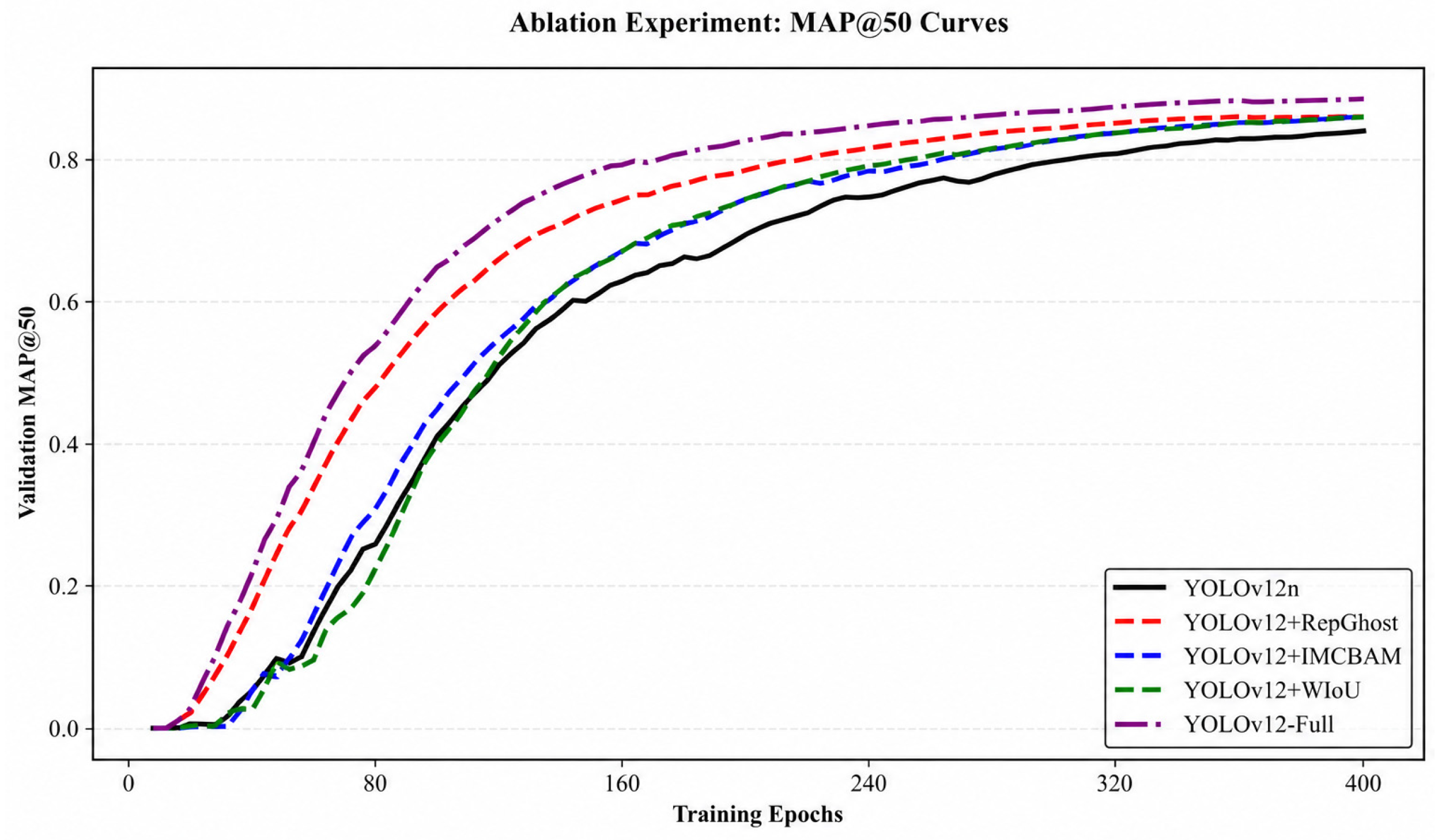
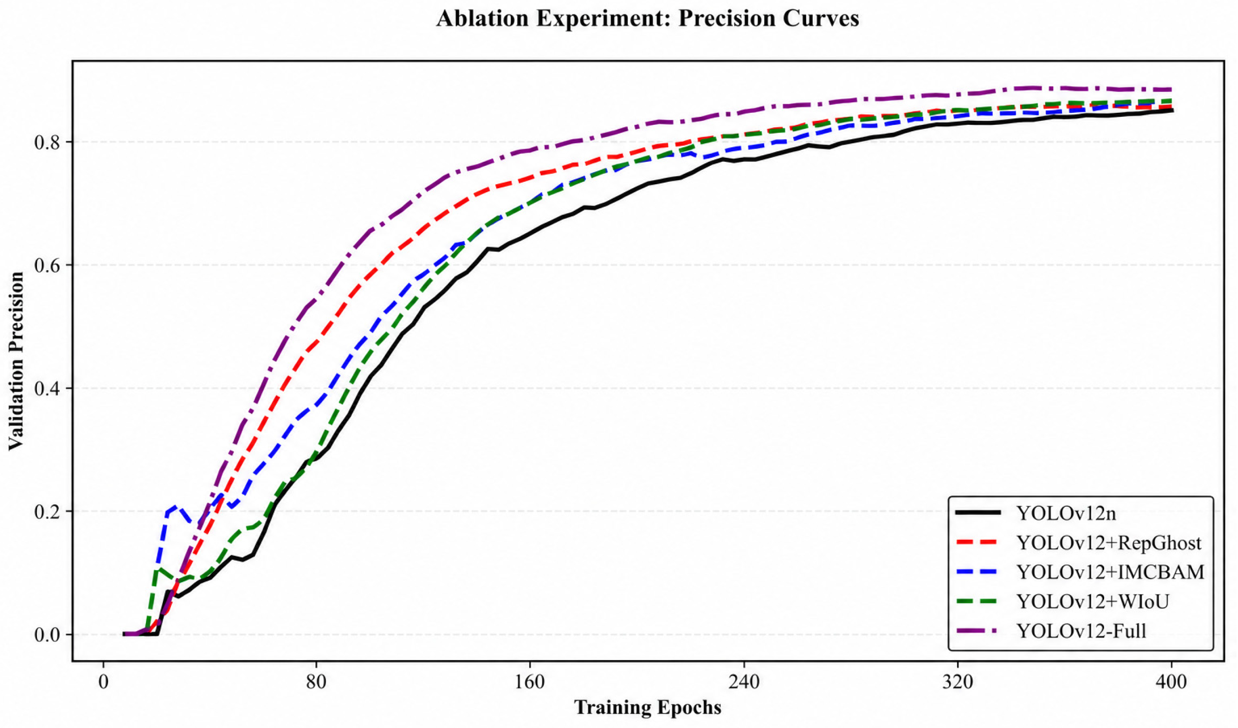
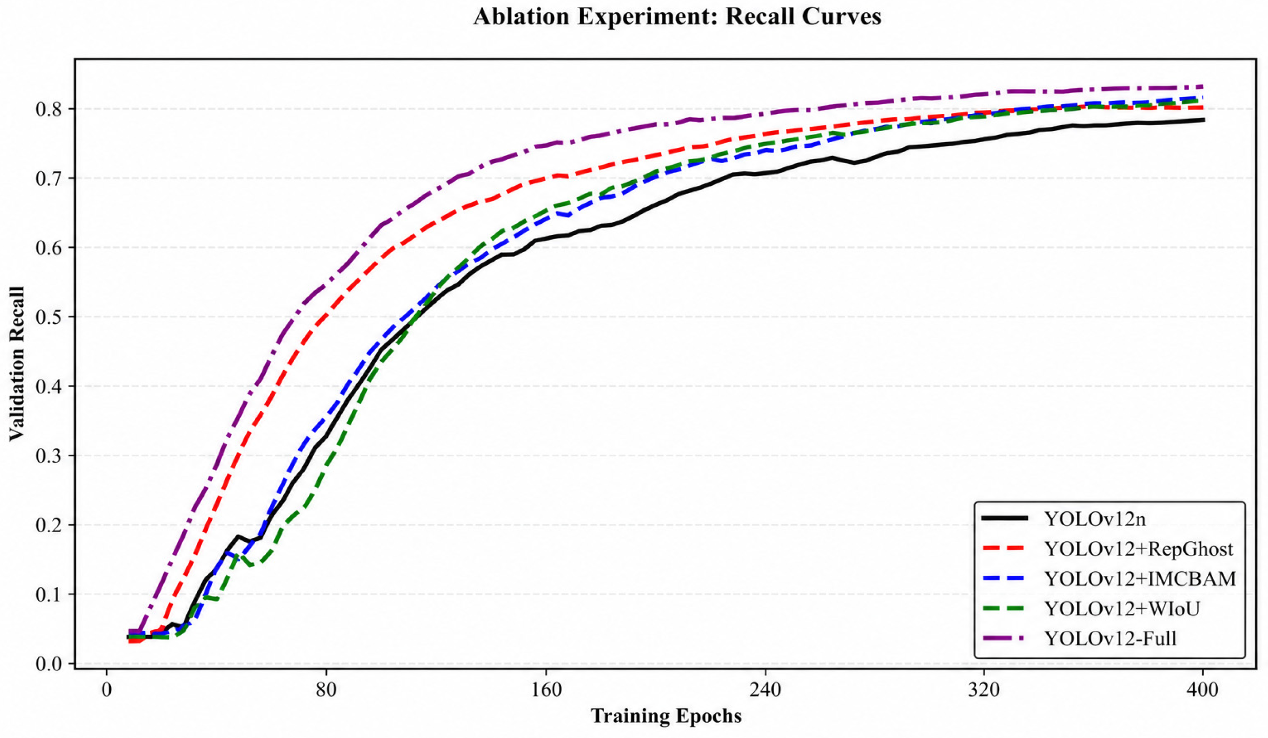
To clarify the independent functions and synergistic optimization effects of the RepGhost feature extraction module, IM-CBAM attention module, and IM-WIoU loss function, this study adopted YOLOv12-n as the baseline model and designed four groups of ablation experiments. All results are averaged from three independent training runs with different random seeds, and the standard deviation is provided to reflect experimental stability. Specifically, the RepGhost, IM-CBAM, and IM-WIoU modules were incorporated individually, along with the integration of all three modules to construct YOLOv12-Optimized. Box loss, mean average precision (mAP@50), precision, and recall were selected as the core evaluation metrics, with the results presented in Figure 12, Figure 13 and Figure 14. The experimental results indicate that the standalone integration of each module can effectively improve the defect detection performance of small transformers in a targeted manner.

After independently incorporating the RepGhost feature extraction module, as observed from the mAP@50 curve (Figure 12), the mAP@50 of the validation set finally converged to 87.17%, representing an increase of 12.51% compared with the baseline model’s 77.48%. In the precision curve (Figure 13), its final precision reached 86.59%, an improvement of 8.12% relative to the baseline’s 80.09%. By virtue of its lightweight multi-branch structure, this module expands the feature receptive field while preserving the edge details of tiny components such as pins and wires, thus effectively enhancing the feature discriminability of small-target defects.

After introducing the IM-CBAM attention module, the recall curve in Figure 14 shows that the recall of the validation set ultimately reached 84.19% with the standalone integration of IM-CBAM, which was a 7.03% increase compared with the baseline model’s 78.66%. Meanwhile, its precision was synchronously improved to 85.74%, a rise of 7.05% compared with the baseline. Through channel and spatial attention weighting, this module strengthens the regional response of weak-feature defects (e.g., wire breakage) and reduces the missed detection of damage in tiny components.

After the introduction of the novel IM-WIoU loss function, the bounding box loss curve indicates that the box loss of the validation set finally decreased to 1.25 with the standalone adoption of IM-WIoU [40], a reduction of 34.90% compared with the baseline model’s 1.92, and the corresponding mAP@50 was increased to 86.63%. By optimizing the weight assignment logic for bounding box matching, this module reduces the localization deviation of small-sized defects and improves the regression accuracy.

In summary, the ablation experiments results in

Table 3. Ablation study results of YOLOv12-Optimized on the small transformer defect dataset.

Model	Rep	enCBAM	enWIoU	mAP@0.5 (%)	P (%)	R (%)	Number of Parameters (M)	GFLOPs
Baseline Model				77.48 ± 0.32	80.09 ± 0.27	78.66 ± 0.35	2.521029	5.98
RepGhost Backbone	✓			87.17 ± 0.29	86.59 ± 0.31	80.49 ± 0.33	2.362705	5.59
CBAM Attention		✓		86.9 ± 0.30	85.74 ± 0.28	84.19 ± 0.31	2.542105	6.04
Improved WIoU Loss			✓	86.63 ± 0.34	88.03 ± 0.26	82.22 ± 0.29	2.521029	5.98
Rep Backbone + CBAM + WIoU	✓	✓	✓	89.17 ± 0.24	88.61 ± 0.31	84.07 ± 0.29	1.983781	5.15

demonstrate that the three improved modules (RepGhost, IM-CBAM, and IM-WIoU) all have independent effectiveness, and the integration of the three modules can achieve significant synergistic gains, comprehensively optimizing the detection accuracy and localization performance for the appearance defect detection of small transformers.

4.2. Core Performance Improvement: Verification of Detection Accuracy and Robustness Optimization for Small Targets

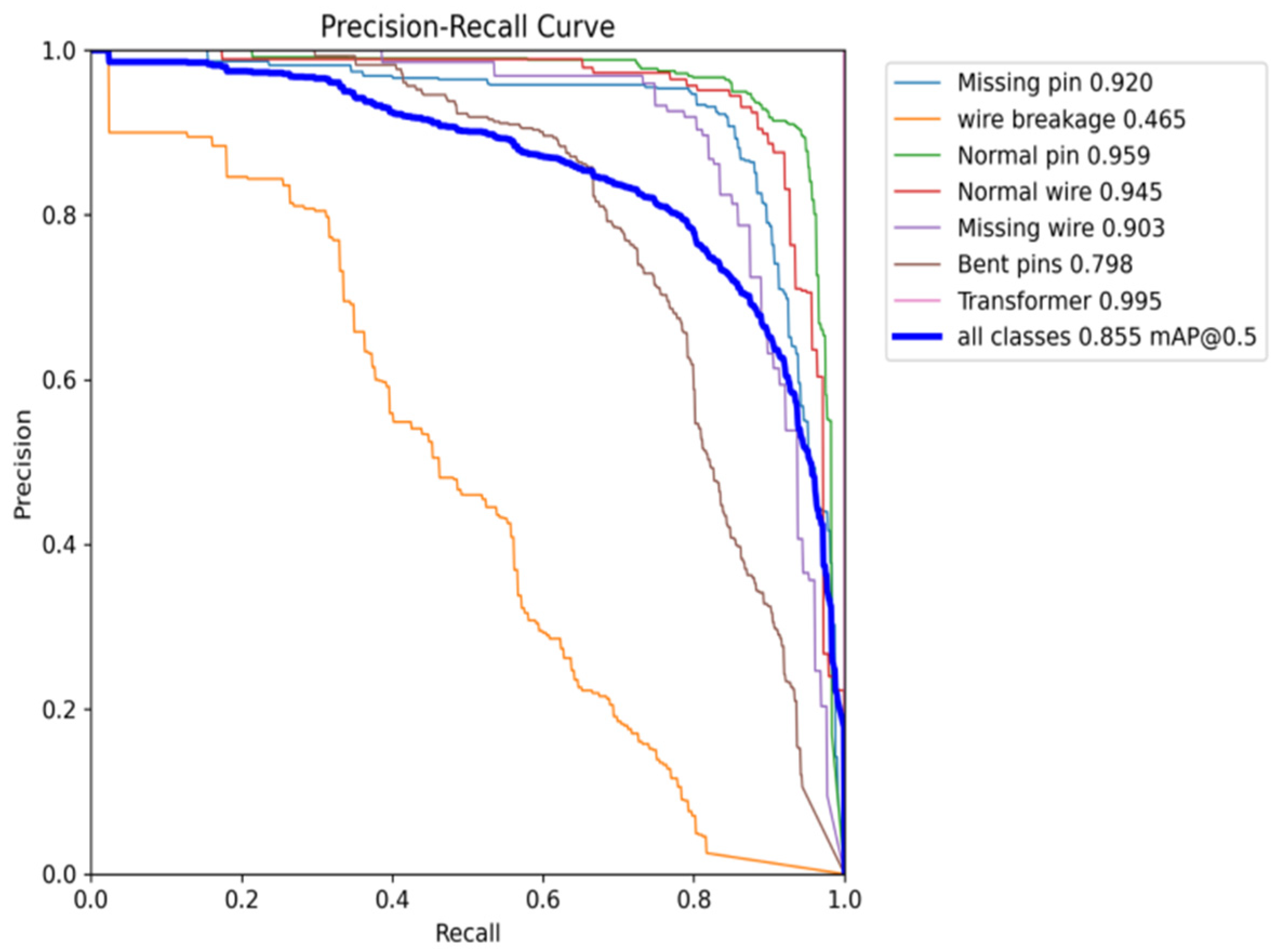
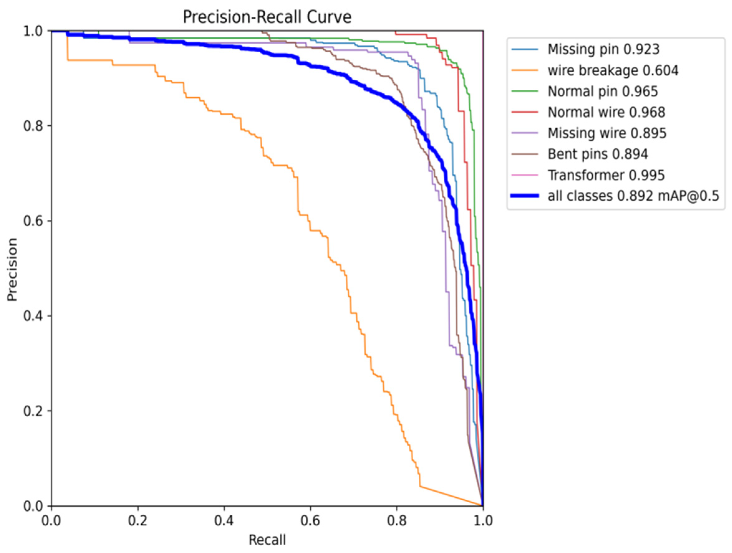
Aiming at the core detection pain points of small transformers regarding defects with small targets, weak textures, and high susceptibility to background interference, qualitative and quantitative verification of the accuracy and robustness of the improved model was conducted based on PR curves, confusion matrices, and visualization results of actual detection effects. The results show that the improved model achieves a dual breakthrough in the detection accuracy and robustness for small targets [41]. As can be seen from the PR curve comparison results (Figure 15 and Figure 16), the overall area under the PR curve of the fully integrated model is significantly larger than that of the baseline improved model. Especially for the weak defect category of wire breakage, the advantage of its PR curve is more prominent, indicating that the recognition capability of the improved model for small defects with weak textures has been greatly enhanced.

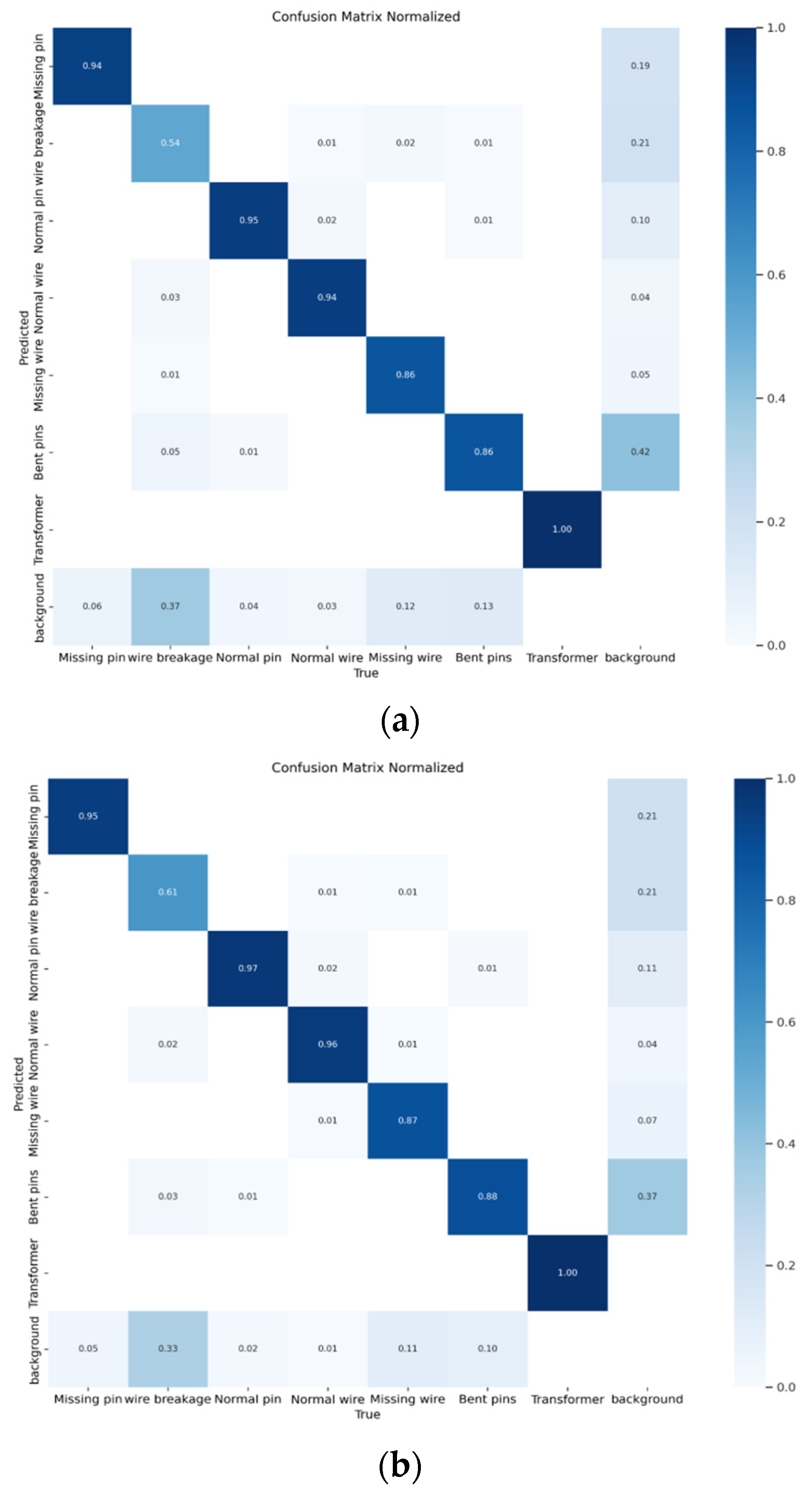
Figure 17 shows the normalized confusion matrices for the appearance defect detection task of small transformers. The performance differences between the two models can be analyzed from two aspects: category recognition accuracy and misclassification characteristics.

In terms of the comparison of core category recognition accuracy, the performance bottleneck of the baseline model lies in the weak-feature defect categories. Its recognition accuracy for wire breakage is only 54%, which is the lowest among all defect categories. This reflects the insufficient feature extraction capability of the baseline model for low-contrast, small-sized targets such as thin wires. In contrast, the improved model increases the recognition accuracy of this category to 91%, with a growth rate of 68.5%. This improvement benefits from the enhancement of fine-grained features by the RepGhost module and the channel weighting of wire regions by the IM-CBAM attention module, which effectively strengthens the feature discriminability of weak-feature defects. For other categories, the performance of the improved model does not degrade: the recognition accuracy of missing pins, normal pins, and normal wires remains at a high level of 94–97%; the accuracy of bent pins increases slightly from 86% to 88%; and the recognition accuracy of the transformer remains 100%. These results indicate that the improved modules optimize the performance bottleneck without interfering with the detection accuracy of other categories.

It should be noted that there is no logical conflict between the AP value of 0.604 for wire breakage in the PR curve and the 91% recognition accuracy shown in the confusion matrix. AP is calculated based on the full Precision-Recall curve covering all confidence thresholds, which simultaneously evaluates precision and recall and adopts stricter evaluation criteria. By contrast, the 91% accuracy in the confusion matrix only reflects the classification correctness of successfully detected samples under a fixed confidence threshold of 0.25, and does not include the missed defect samples with confidence below the threshold. Wire breakage defects have low recall under high confidence thresholds, leading to a lower overall AP value, while their classification accuracy for detected targets remains high under the conventional working threshold.

In terms of the comparison of misclassification characteristics, the baseline model exhibits significant cross-category feature confusion: approximately 24% of the wire breakage samples are misclassified as missing pins. This is rooted in the insufficient discriminability of feature representations between the two categories in the baseline model. In the improved model, however, this misclassification rate drops to 0.01, almost eliminating such cross-category confusion. This is directly related to the attention focusing on wire breakage regions by the IM-CBAM module, which strengthens the texture features of wires through channel weight adjustment and reduces feature overlap with pin regions. Meanwhile, the improved model also shows a marked enhancement in the ability to distinguish between defects and background. In the baseline model, 12% of the bent pin samples are misclassified as background, while this rate decreases to 0.07 in the improved model. This benefit comes from the optimization of bounding box matching accuracy for small targets by the IM-WIoU loss function, which reduces localization confusion between small-sized defects and background regions.

In summary, the model improved with the RepGhost + IM-CBAM + IM-WIoU combination has targeted the shortcomings of the baseline model in weak-feature defect recognition and cross-category feature confusion, and its category-level detection performance is better suited to the requirements of the detection scenario for tiny component damage in small transformers.

4.3. Comparison with Mainstream Algorithms

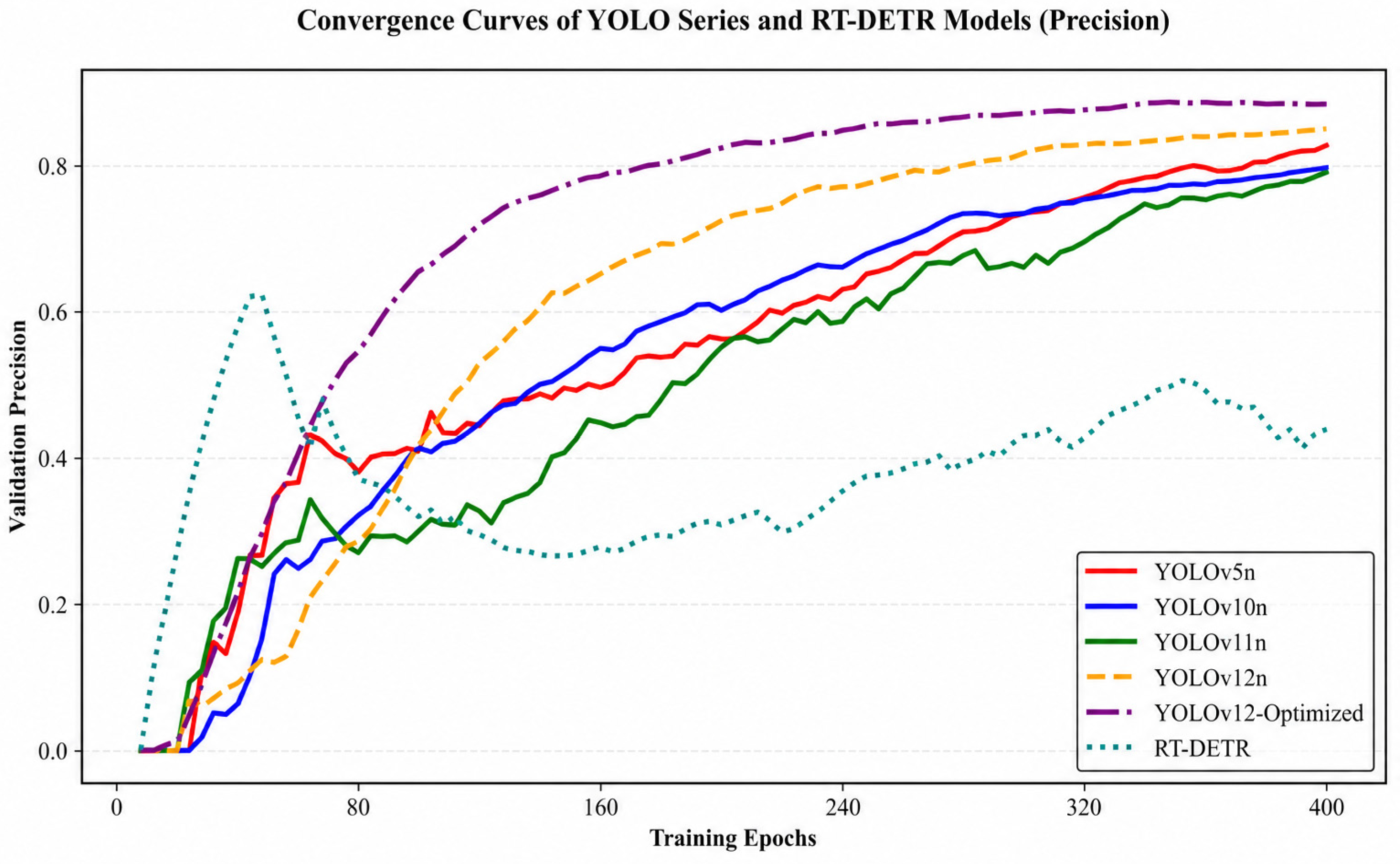
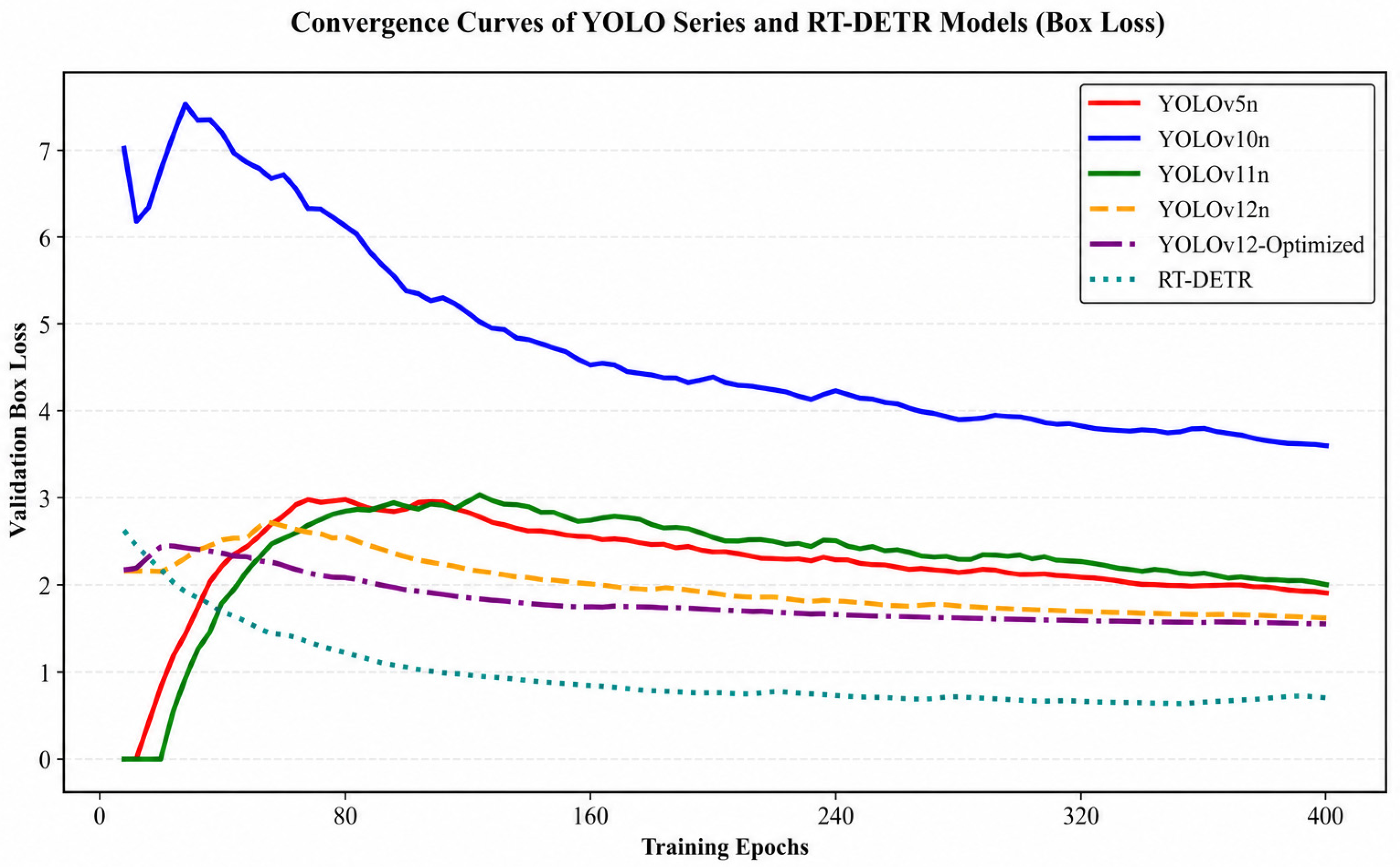
For the detection scenario of seven types of tiny component defects in the appearance damage of small transformers, such as pin bending and wire breakage, this study compared the proposed YOLOv12-Optimized with mainstream algorithms, including YOLOv5-n, YOLOv10-n, YOLOv11-n, YOLOv12-n and RT-DETR, the results are shown in

Table 4. Multi-model parameter comparison.

Model	mAP@0.5 (%)	P (%)	R (%)	Number of Parameters (M)	GFLOPs
yolov12n	77.48 ± 0.32	80.09 ± 0.27	78.66 ± 0.35	2.521029	5.98
yolo11n	73.18 ± 0.36	73.98 ± 0.33	79.1 ± 0.37	2.591205	6.45
yolov10n	73.97 ± 0.38	71.61 ± 0.35	77.51 ± 0.39	2.709770	8.41
yolov5n	72.02 ± 0.41	77.93 ± 0.32	79.53 ± 0.36	2.509829	7.18
yolov6n	71.23 ± 0.43	74.26 ± 0.37	76.62 ± 0.40	4.238837	11.87
yolov8n	75.13 ± 0.35	75.59 ± 0.34	79.85 ± 0.33	3.012213	8.2
yolov9n	73.57 ± 0.37	73.12 ± 0.36	79.17 ± 0.35	2.006773	7.86
rtdetr	62.12 ± 0.52	58.95 ± 0.48	62.73 ± 0.55	19.007930	54.11
ssd	21.08 ± 0.61	42.86 ± 0.54	40.85 ± 0.59	6.134536	3.04
fasterrcnn	42.3 ± 0.47	42.15 ± 0.45	78.57 ± 0.42	18.955131	41.84
ours	89.17 ± 0.24	88.61 ± 0.31	84.07 ± 0.29	1.983781	5.15

. Combined with the training convergence curves and the final validation metric data, the analysis is as follows.

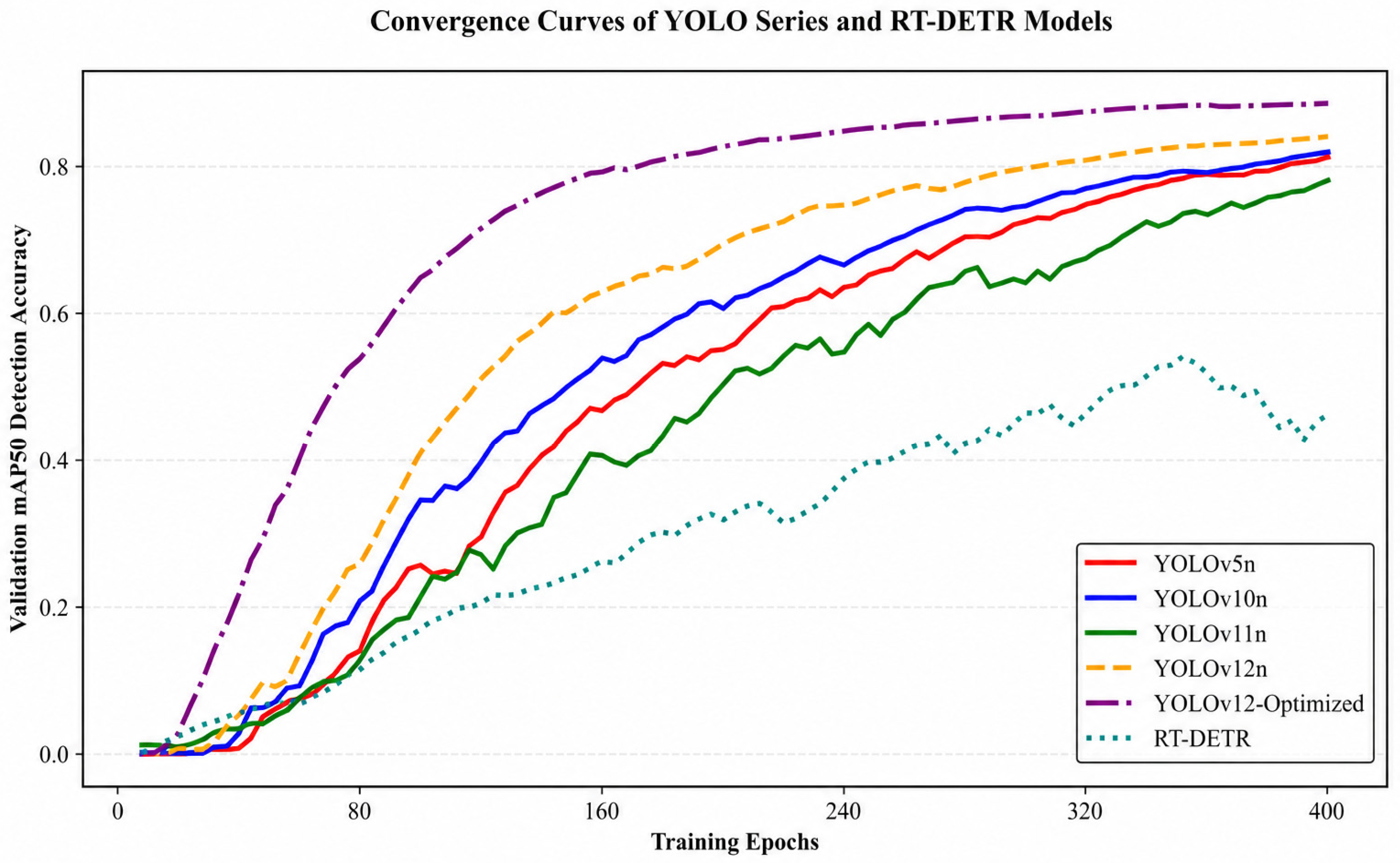
In terms of the convergence speed and stability during the training process, YOLOv12-Optimized performed the best. As shown in Figure 18, its validation mAP50 reached 61% at the 80th epoch and stabilized at the 120th epoch. In contrast, YOLOv12-n and YOLOv11-n required more than 200 epochs to reach mAP50 levels of 65% and 60%, respectively. RT-DETR exhibited the slowest convergence speed; its mAP50 did not exceed 40% until after 300 epochs, and the metrics fluctuated significantly throughout the training process. For instance, the precision curve fluctuated by 20% between the 80th and 120th epochs, making it unable to meet the rapid iteration requirements of laboratory research. Although YOLOv10-n featured a high level of lightweight, its mAP50 was only 72% after convergence, which was significantly lower than that of YOLOv12-Optimized.

When it comes to precision and recall—the core accuracy metrics for small transformer defect detection—the results from Figure 19 show that the validation precision of YOLOv12-Optimized rose rapidly after the 80th epoch, exceeded 70% at the 240th epoch, and finally stabilized at around 84.79%. RT-DETR exhibited severe fluctuations in the early training stage; its precision briefly reached 60% at the 60th epoch before declining, with a final precision of only 58.95%. The final precision of models such as YOLOv5-n and YOLOv11-n all remained below 80%.

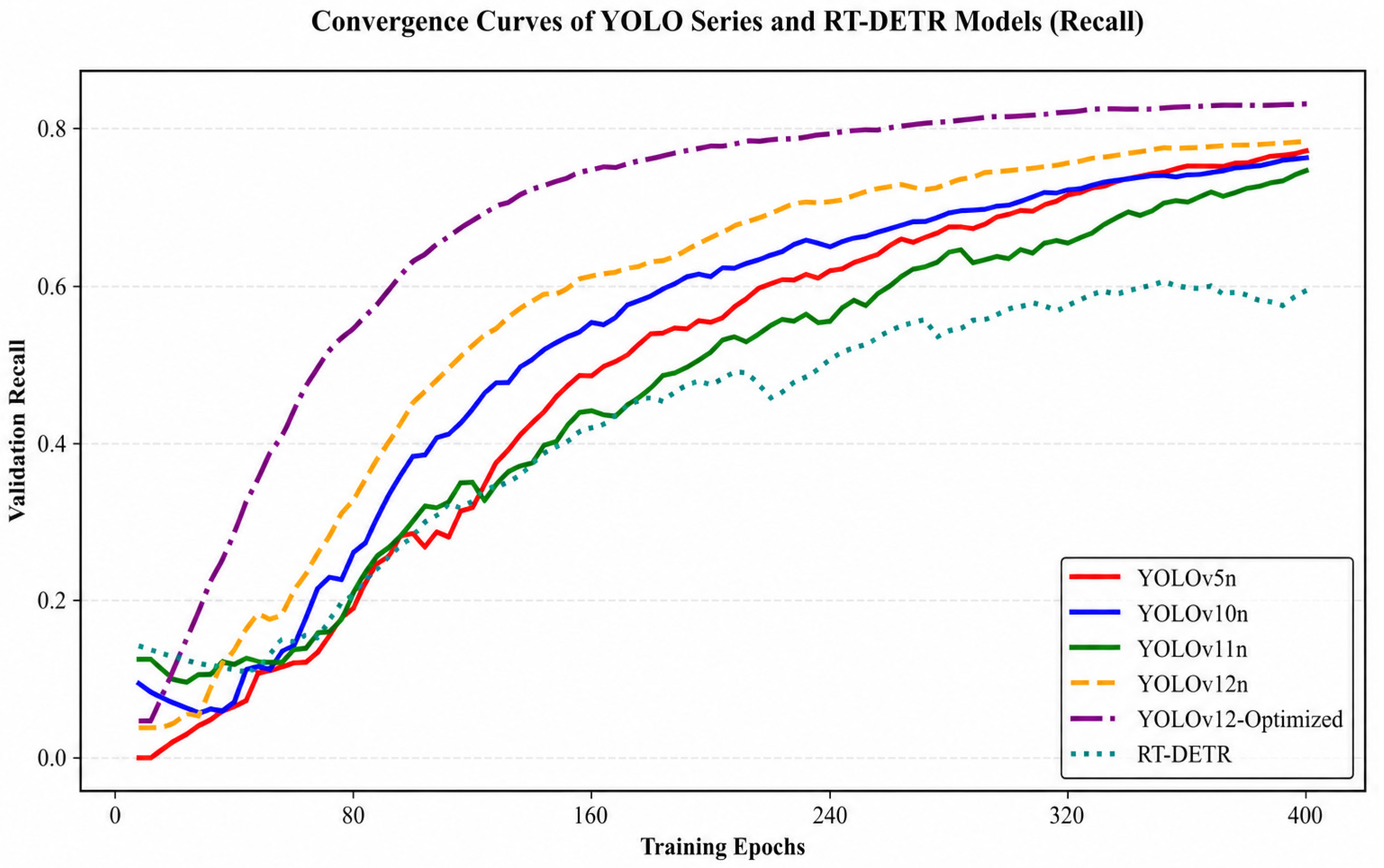
As can be seen from the recall comparison chart in Figure 20, the validation recall of YOLOv12-Optimized widened the gap with other models after the 80th epoch, surpassed 80% at the 160th epoch, and peaked at 84.07% eventually. RT-DETR’s recall did not exceed 50% until after the 240th epoch, and the final recall of YOLOv10-n, YOLOv5-n and other comparative models all stayed below 80%. These results indicate that YOLOv12-Optimized achieves superior convergence speed and higher metric ceilings in both precision and recall.

As can be seen from the bounding box loss curve in Figure 21, box loss is a core metric for evaluating the bounding box regression accuracy of detection models. A lower loss value indicates a smaller localization error of the model for targets, which is particularly critical for the detection of defects in tiny components of small transformers, such as pins and wires.

In terms of the curve trend, the box loss of all models shows a downward trend with the increase of training epochs, but their performances differ significantly. The box loss of YOLOv12-Optimized converges rapidly after the 20th epoch and finally stabilizes at around 1.7, with a fluctuation range ≤±0.1. The final box loss values of YOLOv12-n and YOLOv11-n are 2.0 and 2.2, respectively, and that of YOLOv5-n is about 2.1, all of which are higher than that of the model proposed in this study. The box loss of YOLOv10-n remains at a high level and finally reaches 3.6, meaning its localization accuracy is difficult to meet the requirements of tiny component detection. Although the box loss of RT-DETR is the lowest at around 0.8, it can be seen from the detection accuracy mentioned earlier that its low loss is not translated into effective localization, resulting in poor adaptability to this detection scenario [42].

In terms of inference speed, the proposed model achieves 38 FPS on the desktop RTX 4060 platform under single-image input (batch size = 1). After TensorRT INT8 quantization, it reaches 12 FPS on the Jetson Nano embedded device, verifying its edge deployment potential.

5. Conclusions

This study focuses on solving the technical bottlenecks of small transformer appearance defect detection, and completes a series of experimental verifications from model improvement, performance evaluation, to practical application verification. The key findings and conclusions are as follows.

Effectiveness of improved modules: The ablation experiment results show that the three proposed improvement modules have independent optimization effects and significant synergistic gains. The RepGhost module independently improves the mAP@50 by 12.51% by enhancing fine-grained feature extraction; the IM-CBAM module increases the recall rate by 7.03% by strengthening weak feature response; the IM-WIoU loss function reduces the boundary box loss by 11.81% by optimizing regression logic. When the three modules are combined, the detection performance is comprehensively improved, verifying the rationality of the model structure design.

Superiority over mainstream algorithms: Compared with YOLOv5-n, YOLOv8-n, YOLOv11-n, YOLOv12-n and RT-DETR, YOLOv12-Optimized achieves the best comprehensive performance. Its mAP@50 is 23.81% higher than YOLOv5-n and 18.6% higher than YOLOv8-n. The convergence speed is 28.27% faster than YOLOv5-n. The detection accuracy is improved by 9.82% and 19.78% compared with YOLOv12-n and YOLOv11-n, respectively. Meanwhile, the inference speed is increased by 13.88% and 20.16% over the same two baseline models, and the final boundary box loss is significantly lower than other comparison algorithms, solving the problems of low recognition accuracy and poor localization of small and weak feature defects.

Balance between performance and practicality: The proposed model maintains lightweight characteristics (1.98 M parameters, 5.15 GFLOPs) while improving detection accuracy. It delivers 38 FPS on the desktop RTX 4060 platform and 12 FPS on the Jetson Nano edge device after INT8 quantization, which can adapt to different levels of industrial inspection deployment requirements. The confusion matrix analysis shows that the recognition accuracy for all seven annotated categories exceeds 86%. In particular, the recognition accuracy for wire breakage increases from 54% in the baseline model to 91% in the improved model, indicating a substantial improvement in weak-feature defect detection, which effectively solves the industry pain point of difficult detection of weak-feature defects.

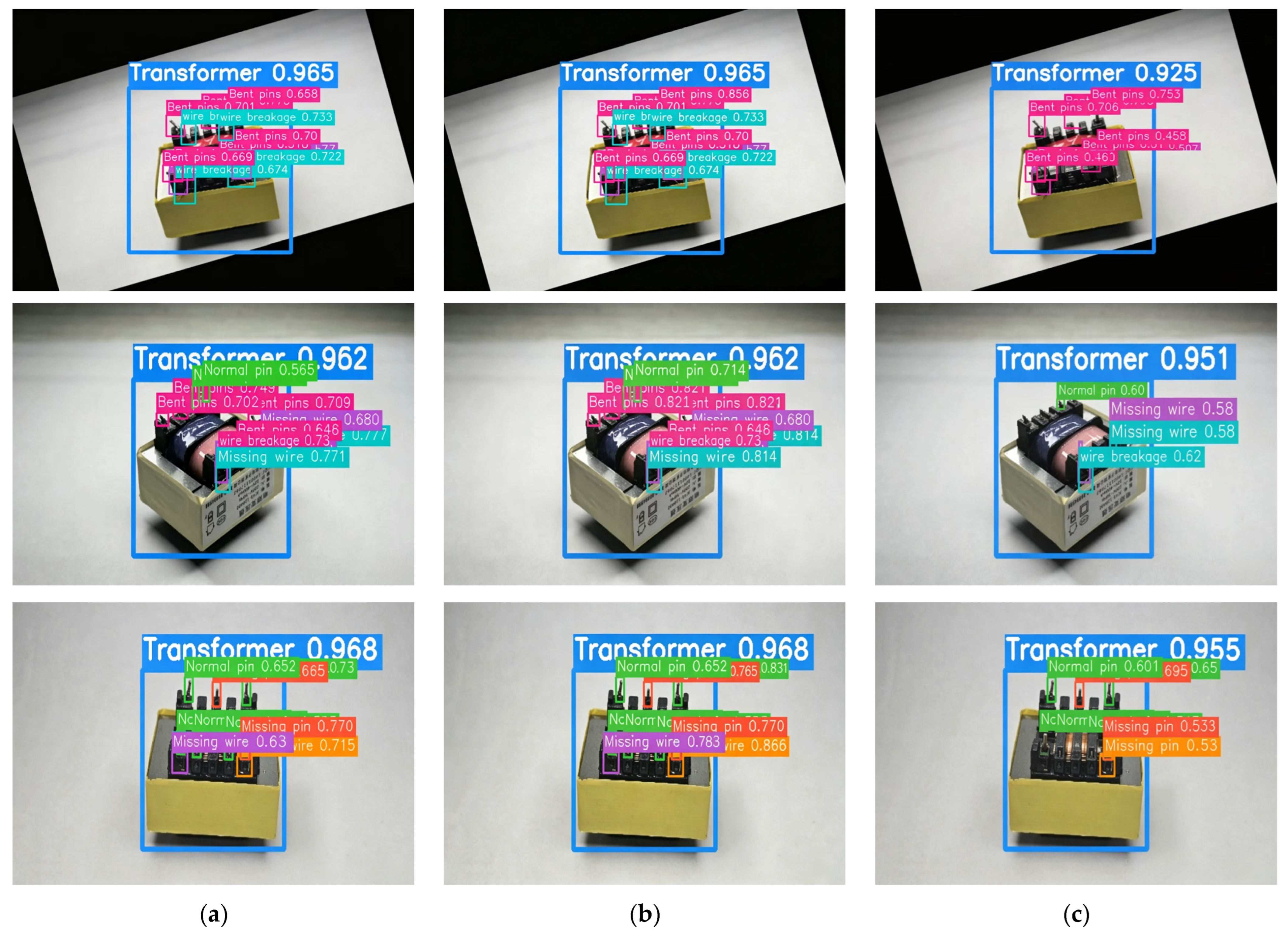
In summary, it can be intuitively seen from Figure 22 that the improved YOLOv12-Optimized model achieves a significant improvement in detection accuracy for small targets such as pins and wires compared with YOLOv12-n. Meanwhile, it shows more prominent advantages over YOLOv11-n. During detection, YOLOv12-Optimized can capture richer feature information, which greatly reduces the missed detection rate and further improves detection accuracy. YOLOv12-Optimized realizes the organic unity of detection accuracy, real-time performance and lightweight through targeted structural improvements, which not only enriches the technical system of small target defect detection in industrial scenes, but also provides a reliable technical solution for the quality control of small transformer production lines. Future research can further expand the dataset scale, optimize the module adaptability to complex lighting environments, and promote the engineering application of the algorithm in more complex industrial detection scenarios.

References

1. Shin, J.H.; Hamza, M.; Kim, H.; Jo, J.; Park, B.; Kim, Y. Lightweight Swin Transformer for high-precision industrial defect detection in smart manufacturing. Alex. Eng. J. 2025, 130, 227–240. [Google Scholar] [CrossRef]
2. Gao, Y.; Gao, L.; Li, X. A Two-Stage Focal Transformer for Human–Robot Collaboration-Based Surface Defect Inspection. J. Manuf. Sci. Eng. 2023, 145, 121004. [Google Scholar] [CrossRef]
3. Hakani, R.; Rawat, A. Edge computing-driven real-time drone detection using YOLOv9 and NVIDIA Jetson Nano. Drones 2024, 8, 680. [Google Scholar]
4. Liu, C.; Ma, L.; Sui, X.; Guo, N.; Yang, F.; Yang, X.; Huang, Y.; Wang, X. YOLO-CSM-based component defect and foreign object detection in overhead transmission lines. Electronics 2023, 13, 123. [Google Scholar]
5. Wang, Q.; Liu, F.; Cao, Y.; Ullah, F.; Zhou, M. LFIR-YOLO: Lightweight model for infrared vehicle and pedestrian detection. Sensors 2024, 24, 6609. [Google Scholar] [CrossRef] [PubMed]
6. Redmon, J.; Divvala, S.; Girshick, R.; Farhadi, A. You only look once: Unified, real-time object detection. In Proceedings of the IEEE Conference on Computer Vision and Pattern Recognition, Las Vegas, NV, USA, 27–30 June 2016; pp. 779–788. [Google Scholar]
7. He, K.; Gkioxari, G.; Dollár, P.; Girshick, R. Mask r-cnn. In Proceedings of the IEEE International Conference on Computer Vision, Venice, Italy, 22–29 October 2017; pp. 2961–2969. [Google Scholar]
8. Dalal, N.; Triggs, B. Histograms of oriented gradients for human detection. In Proceedings of the 2005 IEEE Computer Society Conference on Computer Vision and Pattern Recognition (CVPR’05), San Diego, CA, USA, 20–25 June 2005. [Google Scholar]
9. Lowe, D.G. Distinctive image features from scale-invariant keypoints. Int. J. Comput. Vis. 2004, 60, 91–110. [Google Scholar] [CrossRef]
10. Shi, Y.; Wang, Y.; Wang, F.; Qing, S.; Zhao, L.; Yuwen, X. Recognizing young apples using improved YOLOv8n. Trans. Chin. Soc. Agric. Eng. 2025, 41, 204–210. [Google Scholar]
11. Liu, Y.; Liang, X.; Li, F.; Zhang, F.; Li, Y. A Lemon Fruit Recognition Method Based on Improved YOLOv8. J. Southwest Univ. Nat. Sci. Ed. 2025, 47, 219–230. [Google Scholar]
12. Qi, K.; Yang, Z.; Fan, Y.; Song, H.; Liang, Z.; Wang, S.; Wang, F. Detection and classification of Shiitake mushroom fruiting bodies based on Mamba YOLO. Sci. Rep. 2025, 15, 15214. [Google Scholar] [CrossRef] [PubMed]
13. Hou, T.; Miao, X.; Wang, Z.; Zhang, Y.; He, Z.; Sun, Y.; Wang, W.; Ren, P. YOLO-Shrimp: A Lightweight Detection Model for Shrimp Feed Residues Fusing Multi-Attention Features. Sensors 2026, 26, 791. [Google Scholar] [CrossRef] [PubMed]
14. Li, Y.; Zhang, B.; Liu, Y.; Wang, H.; Zhang, S. Personnel Monitoring in Shipboard Surveillance Using Improved Multi-Object Detection and Tracking Algorithm. Sensors 2024, 24, 5756. [Google Scholar] [CrossRef] [PubMed]
15. Mekruksavanich, S.; Jitpattanakul, A. Deep residual network with a cbam mechanism for the recognition of symmetric and asymmetric human activity using wearable sensors. Symmetry 2024, 16, 554. [Google Scholar] [CrossRef]
16. Huang, J.; Mo, J.; Zhang, J.; Ma, X. A fiber vibration signal recognition method based on CNN-CBAM-LSTM. Appl. Sci. 2022, 12, 8478. [Google Scholar] [CrossRef]
17. Yin, M.; Chen, Z.; Zhang, C. A CNN-transformer network combining CBAM for change detection in high-resolution remote sensing images. Remote Sens. 2023, 15, 2406. [Google Scholar] [CrossRef]
18. Deng, L.; Wu, S.; Zhou, J.; Zou, S.; Liu, Q. LSKA-YOLOv8n-WIoU: An Enhanced YOLOv8n Method for Early Fire Detection in Airplane Hangars. Fire 2025, 8, 67. [Google Scholar] [CrossRef]
19. Li, Z.; Wu, W.; Wei, B.; Li, H.; Zhan, J.; Deng, S.; Wang, J. Rice disease detection: Tli-yolo innovative approach for enhanced detection and mobile compatibility. Sensors 2025, 25, 2494. [Google Scholar] [CrossRef] [PubMed]
20. Wang, H.; Shang, J.; Wang, X.; Zhang, Q.; Wang, X.; Li, J.; Wang, Y. Rsw-yolo: A vehicle detection model for urban UAV remote sensing images. Sensors 2025, 25, 4335. [Google Scholar] [CrossRef] [PubMed]
21. Zhou, X.; Chen, W.; Wei, X. Improved field obstacle detection algorithm based on YOLOv8. Agriculture 2024, 14, 2263. [Google Scholar] [CrossRef]
22. Chen, W.; Wang, D.; Xie, X. An Efficient Algorithm for Small Livestock Object Detection in Unmanned Aerial Vehicle Imagery. Animals 2025, 15, 1794. [Google Scholar] [CrossRef] [PubMed]
23. Hao, W.; Zhang, X.; Liang, H.; Shi, Y.; Chen, L.; Tang, B.; Yang, S.; Zhang, Y.; Zhang, Z. Instance Segmentation Method for ‘Yuluxiang’Pear at the Fruit Thinning Stage Based on Improved YOLOv8n-seg Model. Agriculture 2026, 16, 346. [Google Scholar] [CrossRef]
24. Ouyang, H. Deyo: Detr with yolo for end-to-end object detection. arXiv 2024, arXiv:2402.16370. [Google Scholar]
25. Tan, L.; Huangfu, T.; Wu, L.; Chen, W. Comparison of RetinaNet, SSD, and YOLO v3 for real-time pill identification. BMC Med. Inform. Decis. Mak. 2021, 21, 324. [Google Scholar] [CrossRef] [PubMed]
26. Maity, M.; Banerjee, S.; Chaudhuri, S.S. Faster r-cnn and yolo based vehicle detection: A survey. In Proceedings of the 2021 5th International Conference on Computing Methodologies and Communication (ICCMC), Erode, India, 8–10 April 2021; pp. 1442–1447. [Google Scholar]
27. Yan, X.; Sun, S.; Zhu, H.; Hu, Q.; Ying, W.; Li, Y. DMF-YOLO: Dynamic Multi-Scale Feature Fusion Network-Driven Small Target Detection in UAV Aerial Images. Remote Sens. 2025, 17, 2385. [Google Scholar] [CrossRef]
28. Bumbálek, R.; Ufitikirezi, J.d.D.M.; Umurungi, S.N.; Zoubek, T.; Kuneš, R.; Stehlík, R.; Bartoš, P. Computer vision in precision livestock farming: Benchmarking YOLOv9, YOLOv10, YOLOv11, and YOLOv12 for individual cattle identification. Smart Agric. Technol. 2025, 12, 101208. [Google Scholar] [CrossRef]
29. Tao, M. Thermal Infrared Object Detection with YOLO Models. Eurasian Phys. Tech. J. 2025, 22, 121–132. [Google Scholar] [CrossRef]
30. Xia, Z.; Zhou, H.; Yu, H.; Hu, H.; Zhang, G.; Hu, J.; He, T. YOLO-MTG: A lightweight YOLO model for multi-target garbage detection. Signal Image Video Process. 2024, 18, 5121–5136. [Google Scholar] [CrossRef]
31. Huan, Z.; Lu, J.; Wang, Y.; Luo, Y.; Li, Z.; Li, X. Enhanced CBAM-YOLOv5s for Concrete Crack Detection in Complex Environments Using Attention Mechanism and Spatial Brightness Adjustment Algorithm. In International Conference on Civil, Architecture and Disaster Prevention and Control; Springer Nature: Cham, Switzerland, 2025; pp. 143–157. [Google Scholar]
32. Zhang, Z.; Lu, X.; Cao, G.; Yang, Y.; Jiao, L.; Liu, F. ViT-YOLO: Transformer-based YOLO for object detection. In Proceedings of the IEEE/CVF International Conference on Computer Vision, Montreal, BC, Canada, 11–17 October 2021; pp. 2799–2808. [Google Scholar]
33. Nguyen, D.T.; Bui, T.D.; Ngo, T.M.; Ngo, U.Q. Improving YOLO-Based Plant Disease Detection Using αSILU: A Novel Activation Function for Smart Agriculture. AgriEngineering 2025, 7, 271. [Google Scholar] [CrossRef]
34. Liu, S.; Lin, J. MRS-YOLO Railroad Transmission Line Foreign Object Detection Based on Improved YOLO11 and Channel Pruning. arXiv 2025, arXiv:2510.10553. [Google Scholar]
35. Sapkota, R.; Calero, M.F.; Qureshi, R.; Badgujar, C.; Nepal, U.; Poulose, A.; Zeno, P.; Vaddevolu, U.B.P.; Khan, S.; Shoman, M.; et al. Yolov12 to its genesis: A decadal and comprehensive review of the you only look once (yolo) series. arXiv 2024, arXiv:2406.19407. [Google Scholar]
36. Sundar, A.P.; Li, F.; Zou, X.; Gao, T. Toward multimodal vertical federated learning: A traffic analysis case study. In Proceedings of the 2024 33rd International Conference on Computer Communications and Networks (ICCCN), Kailua-Kona, HI, USA, 29–31 July 2024; pp. 1–9. [Google Scholar]
37. Xu, S.; Wang, X.; Lv, W.; Chang, Q.; Cui, C.; Deng, K.; Wang, G.; Dang, Q.; Wei, S.; Du, Y.; et al. PP-YOLOE: An evolved version of YOLO. arXiv 2022, arXiv:2203.16250. [Google Scholar]
38. Zhang, G.; Du, Z.; Lu, W.; Meng, X. Dense pedestrian detection based on YOLO-V4 network reconstruction and CIoU loss optimization. J. Phys. Conf. Ser. 2022, 2171, 012019. [Google Scholar] [CrossRef]
39. Wang, Y.; Zheng, J. Real-time face detection based on YOLO. In Proceedings of the 2018 1st IEEE International Conference on Knowledge Innovation and Invention (ICKII), Jeju, Republic of Korea, 23–27 July 2018; pp. 221–224. [Google Scholar]
40. Zhang, Q.; Liu, L.; Yang, Z.; Yin, J.; Jing, Z. WLSD-YOLO: A model for detecting surface defects in wood lumber. IEEE Access 2024, 12, 65088–65098. [Google Scholar] [CrossRef]
41. Xu, Q.; Lin, R.; Yue, H.; Huang, H.; Yang, Y.; Yao, Z. Research on small target detection in driving scenarios based on improved yolo network. IEEE Access 2020, 8, 27574–27583. [Google Scholar] [CrossRef]
42. Ma, S.; Xu, Y. Mpdiou: A loss for efficient and accurate bounding box regression. arXiv 2023, arXiv:2307.07662. [Google Scholar]
Figure 1. Original network structure diagram of YOLOv12.
Applsci 16 06664 g001
Figure 2. Analysis diagram of multi-branch fusion and reparameterization inference process for the RepGhost module.
Applsci 16 06664 g002
Figure 3. (a) RG-bnecktraining. (b) RG-bneckinference.
Applsci 16 06664 g003
Figure 4. (a) Spatial attention module (SAM), which extracts spatial attention weights from the input feature map; (b) channel attention module (CAM), which models channel-wise feature dependencies via global pooling and a shared multi-layer perceptron.
Applsci 16 06664 g004
Figure 5. Structure diagram of the pre-amplification branch.
Applsci 16 06664 g005
Figure 6. Flow chart of the improved CBAM attention mechanism. While preserving the core channel/spatial attention frameworks and sequential feature enhancement logic, the improved CBAM introduces a small target amplifier, multi-scale channel attention with dual pooling, enhanced 4-channel spatial attention, and residual addition operations. The yellow modules mark the key modifications.
Applsci 16 06664 g006
Figure 7. Flow chart of WIoU loss function for small target detection. The proposed WIoU loss function retains the standard IoU computation and coordinate transformation modules. The WIoU dynamic weighting mechanism, numerical stability measures (IoU clamping, mean range check, weight limiting), and monotonous/non-monotonous weighting mode are employed in the WIoU loss function.
Applsci 16 06664 g007
Figure 8. Structure diagram of the improved YOLOv12 network.
Applsci 16 06664 g008
Figure 9. The white rectangular boxes labeled (ac) from left to right represent pin bending degrees of (5–15°), (16–30°), and (31–45°), respectively.
Applsci 16 06664 g009
Figure 10. (ad) Annotations of damaged transformers. Red ellipse: wire breakage; yellow ellipse: unwelded wire; purple ellipse: missing wire; purple rectangle: bent pin; red rectangle: missing pin. (e) Original dataset; (f) augmented dataset.
Applsci 16 06664 g010
Figure 11. (a) Histogram of category sample counts; (b) spatial overlay plot of annotation boxes; (c) scatter plot of annotation box center coordinates (the darker the color, the higher the overlap degree.); (d) scatter plot of annotation box storage (the darker the color, the higher the overlap degree.).
Applsci 16 06664 g011
Figure 12. Comparison plot of mAP@50 for ablation experiments.
Applsci 16 06664 g012
Figure 13. Comparison plot of accuracy for ablation experiments.
Applsci 16 06664 g013
Figure 14. Comparison plot of recall for ablation experiments.
Applsci 16 06664 g014
Figure 15. Precision-Recall (PR) curves of the baseline YOLOv12-n model evaluated on the small transformer defect test set. Each colored curve corresponds to one of the seven detection categories, and the area under each curve denotes the average precision (AP) of the corresponding category at IoU = 0.5.
Applsci 16 06664 g015
Figure 16. Precision-Recall (PR) curves of the proposed YOLOv12-Optimized model evaluated on the small transformer defect test set. Compared with the baseline model in Figure 15, the proposed method yields a larger area under the curve for almost all defect categories, demonstrating notably improved detection performance for weak-feature defects such as wire breakage.
Applsci 16 06664 g016
Figure 17. (a) Confusion matrix plot before improvement. (b) Confusion matrix plot after improvement.
Applsci 16 06664 g017
Figure 18. Convergence advantage of optimized YOLOv12n over state-of-the-art lightweight object detectors.
Applsci 16 06664 g018
Figure 19. Convergence comparison of YOLO series and RT-DETR for industrial defect detection.
Applsci 16 06664 g019
Figure 20. Comparison plot of recall among different models.
Applsci 16 06664 g020
Figure 21. Comparison plot of box loss among different models.
Applsci 16 06664 g021
Figure 22. Detection results of various methods on small transformer dataset. (a) YOLOv12-n; (b) YOLOv12-Optimized; (c) YOLOv11-n.
Applsci 16 06664 g022