1. Introduction
1.1. Clinical Context and Motivation
Retinal diseases constitute a major global health burden. The World Health Organization estimates that approximately 2.2 billion people live with some form of vision impairment, of which roughly 1 billion cases are preventable [
1]. Among the leading causes of vision loss are age-related macular degeneration (AMD), diabetic macular edema (DME), and retinal vascular disorders such as retinal vein occlusion (RVO) and retinal artery occlusion (RAO) [
2]. These pathologies differ substantially in their clinical prevalence, with common conditions such as AMD encountered routinely in ophthalmic practice, while disorders such as RAO and vitreomacular interface disease (VID) remain comparatively rare. This inherent class imbalance of retinal pathology distributions in real ophthalmic centers directly motivates the methodological focus of the present work, in which classifiers must remain reliable on rare conditions despite limited training data.
Optical coherence tomography (OCT) is the primary imaging modality used in retinal diagnostics, providing high-resolution, non-invasive cross-sectional visualization of retinal layers [
3]. Despite widespread clinical adoption, manual interpretation remains time-consuming and requires substantial specialist expertise. Automated screening systems based on artificial intelligence have therefore emerged as complementary tools supporting early detection and triage of urgent cases [
4].
1.2. Deep Learning Approaches to OCT Classification
Early deep learning (DL) approaches to retinal OCT classification were dominated by convolutional neural networks (CNNs). Architectures such as ResNet, VGG-16, Inception, and DenseNet served as standard backbones for transfer learning from ImageNet to OCT classification tasks [
5]. While these methods achieved competitive accuracy on small-scale benchmarks, they remained constrained by the limited receptive field of CNN architectures and their inability to model long-range spatial dependencies efficiently.
The introduction of self-attention mechanisms [
6] and Vision Transformers (ViT) [
7] marked a paradigm shift in computer vision. ViT treats an image as a sequence of fixed-size patches, processed through global self-attention to capture long-range spatial dependencies without convolutional operations. To address ViT’s quadratic computational complexity and weak inductive biases, Liu et al. [
8] proposed the Swin Transformer, a hierarchical architecture employing local self-attention within shifted windows. This design preserves multi-scale modeling capability while reducing computational complexity to linear in image resolution and has consistently outperformed both vanilla ViT and earlier CNN baselines on OCT classification benchmarks.
Recent OCT-specific transformer adaptations explore three converging directions. Dutta et al. [
9] proposed Conv-ViT, a hybrid architecture in which CNNs extract local textural features while a ViT captures global contextual relationships. Saraei and Kozak [
10] introduced ViT-2SPN, a dual-stream self-supervised pretraining framework for retinal OCT classification. Karn and Abdulla [
11] proposed the Dual Scale Twin Vision Transformer (DST-ViT), which combines two patch scales with a Twin Transformer architecture, achieving 99.92% accuracy on the OCT2017 benchmark. Despite these strong reported results, the cited works share three common limitations relevant to clinical deployment: (1) evaluation predominantly on the four-class, balanced OCT2017 dataset, which under-represents the diversity of retinal pathologies encountered in practice; (2) absence of training objectives explicitly designed to address class imbalance; and (3) limited cross-validation (CV) rigor—most studies report results on single train/test splits, leaving fold-to-fold variance unmeasured.
1.3. Class Imbalance in Medical Image Classification
Class imbalance is widely recognized as a major challenge for deep classifiers, with systematic studies demonstrating that imbalanced training distributions degrade minority-class performance disproportionately and bias model calibration [
12]. Three principal paradigms have emerged to mitigate this problem.
Re-sampling methods modify the training distribution itself through oversampling minority classes, undersampling majority classes, or synthetic interpolation (SMOTE). While conceptually simple, these methods can introduce overfitting on duplicated minority samples (oversampling) or discard informative examples (undersampling).
Re-weighting methods preserve the original distribution but adjust the per-sample loss according to class frequency. Inverse-frequency weighting is the simplest variant. Cui et al. [
13] proposed a more theoretically grounded Class-Balanced Loss based on the effective number of samples, demonstrating consistent improvements over inverse-frequency weighting on long-tailed CIFAR and ImageNet-LT.
Cost-sensitive loss functions modify the loss landscape itself. Focal Loss (Lin et al. [
14]) down-weights easy examples through a modulating factor that depends on the predicted probability of the true class, originally proposed for dense object detection but widely adopted in imbalanced classification. Label-Distribution-Aware Margin (LDAM) Loss (Cao et al. [
15]) enforces larger margins for minority classes through a label-distribution-aware margin term, with the optional Deferred Re-Weighting (DRW) schedule that delays the application of class weights to mitigate optimization difficulties in early training.
PolyLoss [
16] generalizes both CE and focal loss within a unified polynomial-expansion framework. The loss is decomposed into a polynomial expansion in (1
− pt), where each term is weighted by a tunable coefficient. The simplified Poly-1 variant adds a single hyperparameter ε to the leading polynomial coefficient and has been shown to outperform both CE and focal loss across diverse vision tasks. Crucially, Leng et al. [
16] reported that on datasets with limited samples per class, such as ImageNet-21K, positive values of
ε—opposite in direction to the focal loss paradigm—yielded the best performance, in contrast to balanced ImageNet-1K where smaller or negative ε values were sometimes preferable. Despite this property, to the best of our knowledge, the interaction between PolyLoss and explicit inverse-frequency class weighting under severe imbalance has not been systematically studied.
1.4. OCT Datasets
The number of publicly available OCT datasets supporting more than four disease classes remains limited. The widely adopted Kermany dataset [
17] contains four classes (CNV, DME, Drusen, Normal)—sufficient for benchmarking but insufficient for evaluating clinical screening across the broader pathology spectrum.
The Optical Coherence Tomography Dataset for Image-Based Deep Learning Methods (OCTDL) [
18], comprising over 2000 OCT images across seven diagnostic categories (AMD, DME, ERM, NO, RAO, RVO, VID), better reflects real-world clinical distributions, including pronounced class imbalance—RAO and VID categories contain an order of magnitude fewer samples than AMD or NO. OCTDL was carefully annotated by several experienced retinal specialists, ensuring consistent clinical labeling across the dataset. From the perspective of smaller ophthalmology centers, which encounter rare retinal conditions only sporadically, OCTDL represents a realistic scenario for designing and evaluating screening algorithms.
The complementary OCT-C8 dataset [
19] provides 24,000 images across eight balanced categories, enabling assessment of model behavior on larger, balanced distributions.
Beyond dataset diversity, evaluation rigor warrants attention. Most prior OCT classification studies report results from single train/test splits, providing optimistic point estimates and obscuring fold-to-fold variability. On small medical datasets, this practice has long been shown to produce unreliable performance estimates. Stratified k-fold cross-validation (CV) with confidence intervals (CI)—standard practice in classical machine learning (ML)—remains comparatively rare in transformer-based OCT classification.
1.5. Contributions
Building on the considerations outlined in
Section 1.2,
Section 1.3 and
Section 1.4, this paper presents a comprehensive evaluation of Swin Transformer Base combined with dual-weighted PolyLoss for multi-class OCT classification under severe class imbalance. The methodological pipeline is validated on the OCTDL dataset and on a custom imbalanced subset of OCT-C8 approximating the OCTDL class distribution. The main contributions are as follows:
Loss function ablation. A systematic comparison of eight loss functions: CE, Weighted CE, Focal, Class-Balanced Focal, LDAM, LDAM + DRW, PolyLoss, and Weighted PolyLoss on OCTDL dataset.
Dual-Weighted PolyLoss (DW-PolyLoss) with epsilon ablation. A modification of the original PolyLoss formulation in which inverse-frequency class weights are applied to both the cross-entropy and the polynomial correction term, with a systematic ablation of the correction strength ε under severe imbalance.
Ten-fold CV with logit-averaging ensemble. Stratified 10-fold CV with 95% confidence intervals on an independent held-out test set, followed by a logit-averaging ensemble of all 10-fold models, evaluated using an imbalance-aware metric suite (balanced accuracy, Macro F1, Cohen’s κ, Macro AUROC, ECE) beyond standard accuracy.
Cross-dataset validation on an imbalanced Retinal OCT Image Classification—C8 (OCT-C8) subset. A custom subset of OCT-C8 (eight classes) artificially imbalanced to approximate the OCTDL distribution, evaluated with a balanced held-out test set; a complementary benchmark on the original balanced OCT-C8 is also reported.
Robust ensemble Score-CAM. Four extensions of canonical Score-CAM tailored for transformer-based OCT classification—blur baseline, radial corner suppression, boundary-token down-weighting, and pixel-wise averaging of per-fold heatmaps—jointly addressing Swin- and OCT-specific failure modes of standard saliency methods.
2. Materials and Methods
2.1. Datasets and Cross-Validation Design
The OCTDL dataset [
18] is a publicly available collection of OCT images intended for analysis using DL methods. It was created and made publicly accessible to support research on automatic recognition of retinal pathologies from OCT images. The dataset comprises 2064 OCT images acquired using the Optovue Avanti RTVue XR system, which is characterized by high resolution and scan quality. Each image was annotated in detail by ophthalmology specialists, ensuring the reliability and accuracy of labeling. The images are classified into seven diagnostic categories. The dataset was partitioned using a stratified 80/10/10 split into training, validation, and held-out test subsets, preserving class proportions across all partitions. The held-out test set (n = 213) is kept completely independent throughout all experiments—no training or validation step uses these samples. The exact per-class composition of the split is shown in
Table 1.
The division into diagnostic categories enables the application of multi-class classification methods and the evaluation of the effectiveness of various neural network architectures. The authors of the OCTDL dataset recommend its use as a standard benchmark dataset for comparative studies in the field of retinal image diagnostics and for validating the effectiveness of new DL models. The open availability of this dataset also promotes transparency and reproducibility of research results conducted worldwide. The OCTDL dataset exhibits significant class imbalance—the number of examples for the rarest pathologies (e.g., RAO or VID) is considerably lower than for the most frequent conditions such as AMD or DME, as shown in
Table 1. This data structure not only complicates the classification process but also reflects the real-world situation in medical facilities, where rare retinal conditions occur sporadically, and the number of available diagnostic images is limited.
The second dataset [
19] used in this study is Retinal OCT Image Classification—C8, a publicly available collection of 24,000 OCT images. The dataset covers eight diagnostic categories: age-related macular degeneration (AMD), choroidal neovascularization (CNV), central serous retinopathy (CSR), diabetic macular edema (DME), diabetic retinopathy (DR), drusen, macular hole (MH), and normal retina. In its original form, the dataset is class-balanced, with each category containing an equal number of images, and pre-divided into training (18,400 images), validation (2800 images), and test (2800 images) subsets, with 2300, 350, and 350 images per class, respectively.
To assess transferability of the proposed approach under severe class imbalance comparable to OCTDL, a custom imbalanced subset of OCT-C8 was constructed by sampling, for each class, the number of images specified in
Table 2 from the corresponding train, validation, and test folders of the public OCT-C8 dataset. For each class, the images were drawn without replacement from the alphabetically sorted file list using a fixed-seed (seed = 42) pseudo-random generator, which makes the selection fully reproducible from the public dataset; the per-class counts were chosen to approximate the shape of the OCTDL class distribution. The training and validation pools were imbalanced to an imbalance ratio of approximately 45:1 (closely matching the OCTDL test split), while the held-out test set was kept balanced (350 images per class) to ensure adequate statistical power for per-class metrics. The exact composition of this custom subset is shown in
Table 2.
For 10-fold cross-validation experiments, the OCTDL training and validation sets were merged into a single CV pool (n = 1851), which was then partitioned using stratified k-fold splitting from scikit-learn, ensuring class proportions are maintained in each fold. In each iteration, 9/10 of the CV pool served as training data, and 1/10 as internal validation (used for early stopping and overfitting monitoring). Final evaluation of each fold model was performed on the independent held-out test set (n = 213), ensuring comparability across folds. The same protocol was applied to the OCT-C8 imbalanced subset (CV pool n = 4213, held-out test n = 2800).
2.2. Preprocessing and Augmentation
OCT images, which are inherently monochromatic, were converted to a three-channel format via channel replication to match the pretrained model’s input requirements. All images were resized to 224 × 224 pixels and normalized with channel-wise mean and standard deviation values both set to 0.5. The training augmentation pipeline included random rotation by up to ±10°, random horizontal flipping, color jitter applied to brightness and contrast (factor ±0.1), and random affine translation of up to ±5% of the image width and height. Validation and test sets used only the base transforms (resizing and normalization), without any stochastic augmentation. The same preprocessing and augmentation configuration was applied consistently across all experiments reported in this paper.
2.3. Swin Transformer Base Architecture
The backbone architecture was Swin Transformer Base (model: swin_base_patch4_window7_224), a ViT with shifted-window self-attention [
8]. The model was loaded with ImageNet-1k pretrained weights through the timm library, and the original 1000-class classification head was replaced with a new linear layer matched to the target class count (7 outputs for the OCTDL experiments and 8 outputs for the OCT-C8 cross-dataset evaluation). Key architectural parameters include patch size 4 × 4 pixels, attention window 7 × 7, input resolution 224 × 224 pixels, embedding dimension 128 in the first stage and progressively doubling to [128, 256, 512, 1024] across the four hierarchical stages, stage depths [2, 2, 18, 2] (a total of 24 transformer blocks), and attention heads [4, 8, 16, 32]. Global average pooling is applied to the final 7 × 7 feature map (1024 channels) before the linear classifier. The full network contains approximately 88 million trainable parameters.
2.4. Loss Function: Dual-Weighted PolyLoss (DW-PolyLoss)
PolyLoss extends standard CE loss with a polynomial correction term. Specifically, we adopt the Poly-1 variant (single polynomial term) defined as follows:
where
CE(
x,
y) is the standard CE loss,
pt is the model’s predicted probability for the true class (obtained via softmax), and ε (epsilon) is a hyperparameter controlling the correction strength. The (1 −
pt) term penalizes insufficient model confidence—the further
pt is from 1.0, the larger the penalty, pushing predicted probabilities closer to certainty for correct classes.
The computation proceeds in four stages: first, the per-sample CE loss is calculated with class weights applied independently to each sample; second, the softmax probability distribution over all classes is obtained; third, the predicted probability for the true class pt is extracted; and fourth, the polynomial correction term ε·(1 − pt) is computed. The final loss is the elementwise sum of the CE and polynomial components, averaged across all samples in the batch.
The methodological element introduced here is the dual weighting mechanism. We emphasize that DW-PolyLoss is a deliberately lightweight modification of PolyLoss rather than a new loss family; its specific, previously unexamined element is the symmetric application of the inverse-frequency class weight to both terms of the loss, in contrast to the common practice of weighting only the cross-entropy term. Class weights were calculated as the inverse of class frequency in each fold’s training subset:
w_i = 1/
count_i, then normalized by dividing by the mean weight (
w_i/
mean(
w)), and applied to both the CE component and the polynomial correction term, yielding the following formulation:
This creates a dual correction: for any minority class whose inverse-frequency weight exceeds unity, both the misclassification penalty and the confidence penalty are amplified proportionally to the rarity of that class. The effect is most pronounced for the rarest categories in OCTDL (such as RAO and VID), where the polynomial term and the CE term are simultaneously scaled up, while majority classes (such as AMD) receive sub-unity weights and are correspondingly down-weighted. Crucially, class weights are recomputed independently for each fold since the training composition changes between folds due to the CV split. To the best of our knowledge, this specific interaction between PolyLoss and per-fold inverse-frequency class weighting has not been explicitly examined in prior work.
2.5. Training Configuration
The models were trained using the AdamW [
20] optimizer with an initial learning rate of 5 × 10
−5 and weight decay of 0.01. The learning rate schedule followed cosine annealing with a 2-epoch linear warmup phase starting from 10% of the peak learning rate (5 × 10
−6) and a minimum learning rate floor of 1 × 10
−6. Training was conducted for a maximum of 60 epochs with a batch size of 16, and early stopping with a patience of 7 epochs monitored validation accuracy to prevent overfitting. Mixed precision training (FP16) was enabled to accelerate computation and reduce GPU memory usage. To ensure reproducibility, the random seed was set deterministically for each fold as 42 + fold index, and deterministic computation mode was enabled.
For each fold, the model was initialized with ImageNet-pretrained weights, and the best checkpoint (by validation accuracy) was saved for test set evaluation. The experiments were conducted on a single NVIDIA A100 GPU using the PyTorch 2.11.0 framework with the timm 1.0.27 library for model instantiation and scikit-learn 1.6.1 for CV partitioning and metrics computation.
2.6. Ensemble via Logit Averaging
The 10-fold CV naturally produces 10 fully trained models, which were aggregated into a logit-averaging ensemble rather than selecting a single best fold. For each test image, the raw logit vectors from the K = 10 models are combined by an element-wise mean, and softmax followed by argmax yields the final ensemble prediction. Logit averaging was preferred over probability averaging because logits are not distorted by the exponential softmax transformation, which tends to yield better-calibrated ensemble probabilities when individual models differ in calibration. Since each fold is trained on a different 90% partition of the CV pool, the resulting models exhibit partially uncorrelated errors, and averaging suppresses idiosyncratic mistakes.
2.7. Evaluation Metrics
Given the severe class imbalance in the OCTDL dataset—where the majority class (AMD, 1231 samples) outnumbers the rarest class (RAO, 22 samples) by a factor of 56:1—standard accuracy alone is an insufficient evaluation criterion. A naive classifier predicting only AMD would achieve approximately 60% accuracy while completely failing on all minority classes. Standard practice in imbalanced classification therefore extends evaluation beyond accuracy and per-class precision/recall to include metrics specifically designed to expose performance disparities across classes of vastly different sizes.
The model is evaluated using the following set of metrics:
Accuracy—the proportion of correctly classified samples in the test set.
Balanced Accuracy [
21]—the unweighted mean of per-class recall, giving equal importance to each class regardless of its size.
Macro F1-score—the unweighted average of per-class F1-scores, preventing the majority class from masking poor minority-class performance.
Weighted F1-score—included for comparison with the size-weighted perspective.
Macro AUROC (one-vs-rest)—the discriminative ability of the model independently of the classification threshold, particularly informative under imbalance where threshold selection significantly affects per-class performance.
Cohen’s κ [
22]—agreement beyond chance level, inherently adjusted for class prevalence. The unweighted variant is used because the seven OCTDL diagnostic categories are nominal rather than ordinal; weighted variants assume an ordering between categories that is not justified for distinct retinal pathologies.
Expected Calibration Error (ECE) [
23]—assesses whether the model’s predicted probabilities reliably reflect the empirical accuracy [
24].
The 95% CI values over the 10 folds were computed using the t-distribution with 9 degrees of freedom, following common practice in CV reporting. We acknowledge that this method may be slightly anti-conservative due to the partial dependence between folds; per-class effects with stricter inferential requirements should therefore be interpreted with appropriate caution. Per-class ROC curves were computed for each class in a one-vs-rest scheme and interpolated to a common false-positive-rate grid of 200 points before averaging across folds.
2.8. Score-CAM Interpretability Analysis
To verify that the trained model attends to clinically relevant regions rather than to acquisition artifacts or padding-related boundary effects, Score-CAM [
25] was applied to the 10-fold CV ensemble. Score-CAM is a gradient-free class activation mapping method: per-channel importance weights are obtained by perturbing the input with upsampled activation maps and measuring the resulting change in the target-class probability, avoiding the noisy gradient signal of gradient-based alternatives such as Grad-CAM [
26].
The target layer was the final normalization layer of the last Swin stage, producing a 7 × 7 spatial grid of 1024-dimensional feature vectors that were bilinearly upsampled to the input resolution (224 × 224). The target class for each test image was taken from the logit-averaging ensemble, so that the visualized attention corresponds to the class predicted by the ensemble rather than by any single fold model.
Four extensions of the canonical Score-CAM pipeline were applied to address artifacts specific to transformer architectures and to the OCT imaging domain:
Gaussian-blurred baseline. Instead of a zero baseline, which is out-of-distribution for the trained model, the baseline was a Gaussian-blurred copy of the input (σ = 10), preserving global luminance and texture while removing local features.
Corner suppression. A smooth radial mask centered on the image was multiplied with the final heatmap to attenuate activations outside the central circular region, respecting the physically circular nature of OCT B-scan acquisitions where the corners of the rectangular frame fall outside the actual scan.
Boundary-token down-weighting. Before computing channel-importance scores, tokens at the corners and edges of the 7 × 7 grid were attenuated, mitigating spurious activations that arise from Swin window attention near the image boundary, where attention windows partially extend beyond the input.
Ensemble averaging. Score-CAM was generated independently for each of the 10-fold models with the same ensemble target class, and the per-fold heatmaps were normalized and averaged pixel-wise. This aggregation parallels the logit-averaging strategy of
Section 2.6 and suppresses fold-specific idiosyncrasies in the attention maps.
3. Results
3.1. Ablation Study: Loss Function Comparison
Eight loss functions were compared under identical training conditions on the OCTDL dataset, using stratified 10-fold cross-validation as detailed in
Section 2.1 (
Table 1). The training configuration follows the protocol described in
Section 2, with the loss function being the only varied component. Results are summarized in
Table 3.
The compared objectives correspond to the three imbalance-handling paradigms introduced in
Section 1.3: the unweighted cross-entropy baseline (CE); a re-weighting variant that scales the loss by class frequency (Weighted CE, inverse-frequency weights on the cross-entropy term); cost-sensitive objectives that reshape the loss landscape (Focal, Class-Balanced Focal, LDAM, and LDAM + DRW); and the PolyLoss family (PolyLoss and its single-term-weighted variant, Weighted PolyLoss). Weighted PolyLoss applies the inverse-frequency weight only to the cross-entropy term, leaving the polynomial correction unweighted, and therefore serves as the direct single-term-weighting counterpart to the dual-weighted formulation studied in
Section 3.2.
Across the 10 folds, no single objective dominated the metric suite (
Table 3): CE gave the lowest ECE (0.0363), Weighted CE the highest balanced accuracy (0.9328) and Macro F1 (0.9212) among the fixed losses, and Focal Loss the highest accuracy (0.9540) and AUROC (0.9968), while the margin-based losses (LDAM and LDAM + DRW) reached competitive accuracy but markedly higher ECE (above 0.45). Weighted PolyLoss, which weights only the cross-entropy term, ranked lowest on balanced accuracy (0.8994) and Macro F1 (0.8953).
3.2. DW-PolyLoss with Epsilon Ablation
Building on the loss-function comparison in
Section 3.1, a dedicated sweep was performed on the proposed DW-PolyLoss formulation (Equation (2)) to identify the optimal value of its polynomial-correction coefficient ε. Six values of ε, spanning the mild-to-moderate correction range in steps of 0.1, were evaluated under DW-PolyLoss: ε = 0.5, 0.6, 0.7, 0.8, 0.9, and 1.0. The training protocol matches the 10-fold cross-validation configuration of
Section 3.1. Results are summarized in
Table 4.
Performance varied smoothly with ε (
Table 4). The highest accuracy (0.9577) and the lowest calibration error (ECE 0.0328) were both obtained at ε = 0.8, whereas ε = 0.7 gave the best Macro F1 (0.9229) and AUROC (0.9975), and ε = 0.6 the best balanced accuracy (0.9305); the differences among the top settings were small, generally within one standard deviation across folds. Based on this sweep, ε = 0.8 was selected for all subsequent experiments (
Section 3.3,
Section 3.4,
Section 3.5,
Section 3.6 and
Section 3.7), as it attained the best accuracy and calibration while remaining within 0.25 p.p. of the best balanced accuracy and Macro F1.
3.3. Ten-Fold Stratified CV of DW-PolyLoss (ε = 0.8) on OCTDL
The DW-PolyLoss (ε = 0.8) configuration selected in
Section 3.2 is examined here in more detail under the same 10-fold stratified cross-validation protocol, providing per-fold estimates, 95% confidence intervals, and the aggregated confusion matrix that serve as the basis for the logit-averaging ensemble in
Section 3.4. On a dataset as small as OCTDL (n = 2064), cross-validation gives confidence-bounded estimates by training and evaluating across multiple data partitions, rather than relying on a single split. The resulting metrics are summarized in
Table 5, and
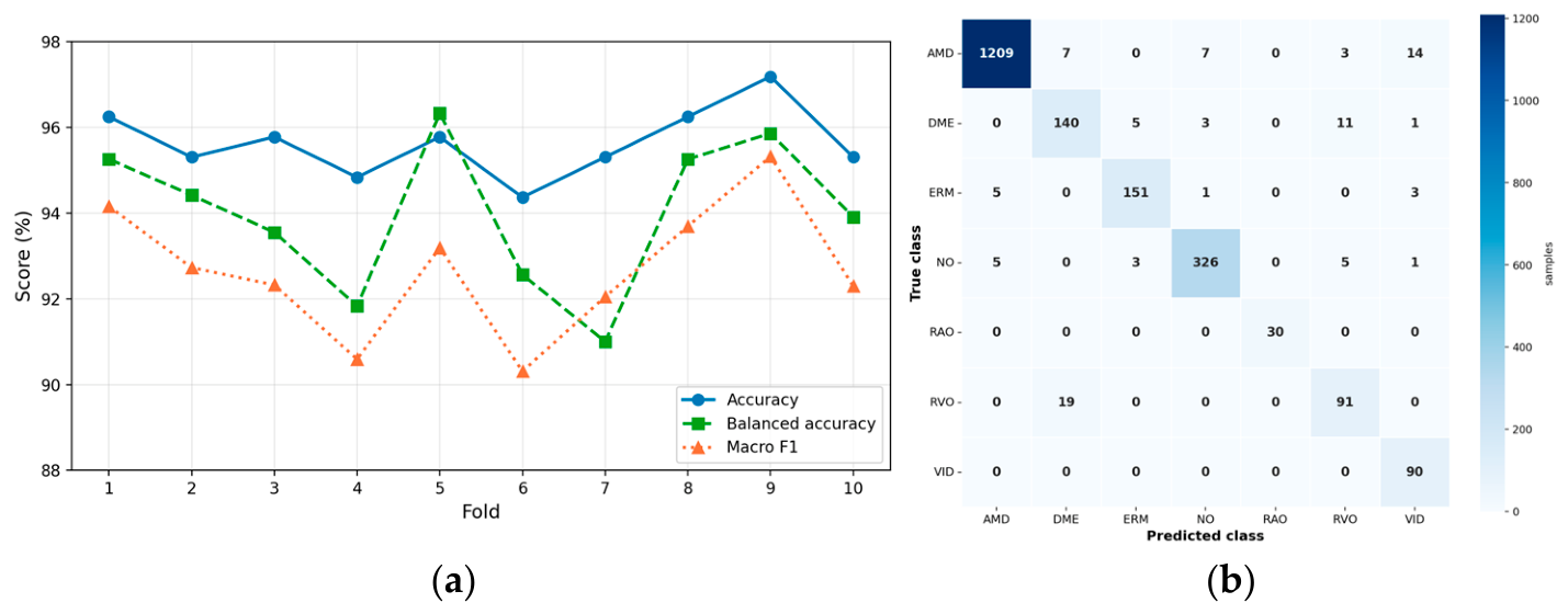
Figure 1 shows the per-fold scores and the aggregated confusion matrix on the held-out OCTDL dataset (n = 213). Because this is an independent training run, the values in
Table 5 differ marginally from the ε = 0.8 entry of the epsilon sweep (
Table 4); the deviations stay below 0.01 on every metric and within the fold-to-fold standard deviation, reflecting the limited run-to-run reproducibility of GPU training rather than any change in configuration.
Performance was stable across folds, with per-fold accuracy ranging from 94.37% to 97.18% and no outlier fold (
Figure 1a). The aggregated confusion matrix (
Figure 1b) shows that the rarest categories were recovered well, with RAO and VID reaching complete recall (30/30 and 90/90), while the residual errors concentrated between the exudative and vascular classes, most notably RVO predicted as DME (19 cases) and a small spread of AMD into VID, DME, and NO.
3.4. Ensemble Model Results of DW-PolyLoss (ε = 0.8) on OCTDL
Building on the 10-fold CV reported in
Section 3.3, an ensemble model was constructed by aggregating predictions from all 10-fold models via logit averaging (see
Section 2.6 for the protocol). Performance relative to the 10-fold CV baseline (mean across single fold models, not the ensemble itself) on the independent held-out test set is reported in
Table 6. This step leverages the trained fold models that would otherwise be discarded after CV evaluation, exploiting their partially uncorrelated errors to yield a single consensus prediction with improved stability and calibration.
Logit averaging improved every metric over the fold average (
Table 6), with the largest gains in the imbalance-aware metrics (Macro F1 +3.00 p.p., balanced accuracy +2.15 p.p.) and a reduction in calibration error from 0.0377 to 0.0315.
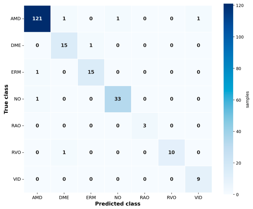
Figure 2 shows the ensemble confusion matrix on the OCTDL held-out test set: 206 of 213 cases were classified correctly, the rarest classes RAO and VID were perfectly recovered (3/3 and 9/9), and the few residual errors were isolated single cases (for example, one AMD predicted as VID and one RVO as DME).
3.5. Comparison with Existing Approaches
Table 7 compares the proposed approach with previously reported results on OCTDL. The cited baselines (ResNet50 and VGG16 [
18]; ViT and BEiT [
27]) were reported on single train/test splits, whereas the proposed approach is given under two protocols: the DW-PolyLoss (proposed) row reports the 10-fold cross-validation mean (
Section 3.3), which is the closest like-for-like comparison with the single-split baselines, and the DW-PolyLoss ensemble (proposed) row reports the logit-averaging ensemble of all 10 fold models. The single-split baseline figures should therefore be read with the caveat that, on a dataset of this size, cross-validated estimates are more reliable than single-split point values.
3.6. Ten-Fold Stratified CV of DW-PolyLoss on OCT-C8
To assess transferability of the proposed approach to a second OCT dataset with a comparable imbalance structure, the DW-PolyLoss (ε = 0.8) configuration was evaluated under 10-fold stratified CV on the custom imbalanced subset of OCT-C8 introduced in
Section 2.1 (
Table 2; CV pool n = 4213 with imbalance ratio ≈ 45:1, held-out balanced test set n = 2800 with 350 images per class). All training hyperparameters, the cross-validation protocol, the ensembling strategy, and the evaluation metrics replicate exactly those used for OCTDL (
Section 2.5,
Section 2.6 and
Section 2.7); only the number of output classes (eight instead of seven) and the dataset itself were changed, ensuring that any differences in performance can be attributed to the dataset rather than to methodological adaptations. Total training time across the 10 folds was 2 h 50 min on a single NVIDIA A100 GPU.
The 10-fold cross-validation results on the balanced OCT-C8 held-out test set are presented in
Table 8. The ensemble improvement is reported in
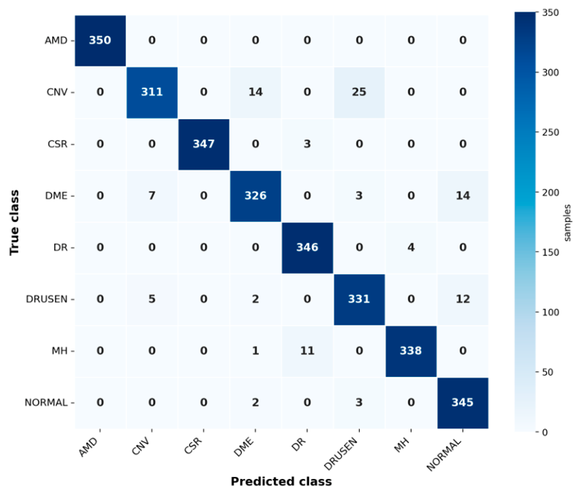
Table 9, and the ensemble confusion matrix is shown in
Figure 3.
Because the held-out test set is balanced by design (350 images per class), Accuracy and Balanced Accuracy are mathematically identical. The comparison of the logit-averaging ensemble against the per-fold average is presented in
Table 9.
Figure 3 shows the confusion matrix of the logit-averaging ensemble on the balanced OCT-C8 held-out test set (n = 2800), enabling per-class inspection of prediction patterns across the eight diagnostic categories.
3.7. Model Interpretability: Score-CAM Analysis
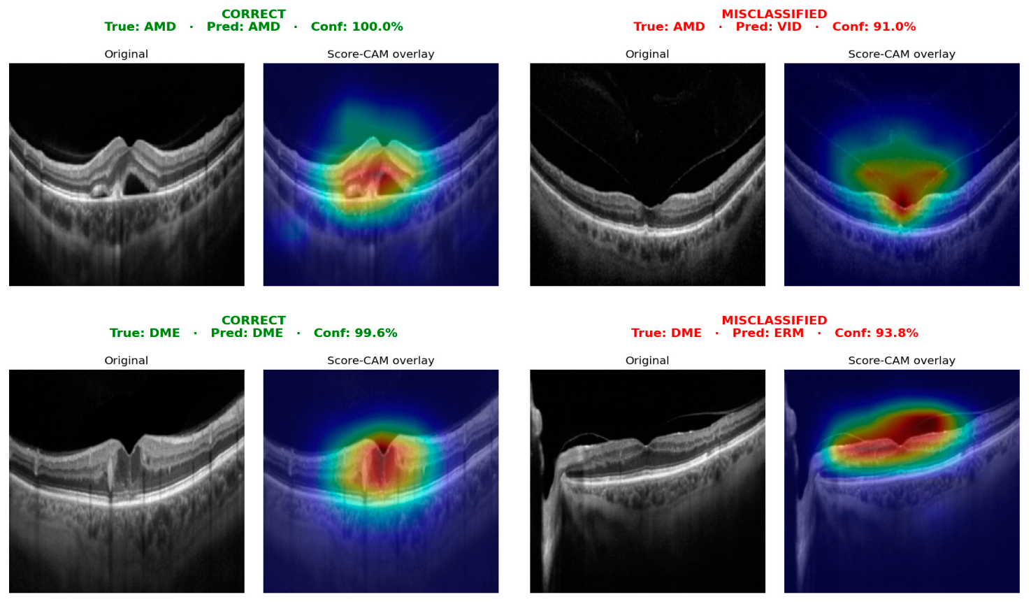
Score-CAM was applied to the 10-fold logit-averaging ensemble on the OCTDL held-out test set (n = 213), following the protocol described in
Section 2.8. Four representative cases are shown in
Figure 4.
4. Discussion
4.1. From Loss Function Ablation to Dual-Weighted PolyLoss
All OCTDL comparisons in this work, the loss-function ablation of
Section 3.1, the epsilon sweep of
Section 3.2, and the final model evaluation, were carried out under 10-fold stratified cross-validation rather than a single train/test split. This choice is dictated by the dataset itself: with only 2064 images and the rarest categories reduced to a handful of cases (RAO, n = 22; VID, n = 76), any single partition places so few minority-class examples in the test set that the measured performance depends heavily on which images happen to fall there, and the small differences between competing losses cannot be separated from this sampling noise. Cross-validation instead rotates every image through both training and testing across the folds and reports per-fold means with 95% confidence intervals, so the differences discussed below reflect properties of the method rather than one fortunate or unfortunate split. Seen in that light, the loss-function ablation is best read not as a search for a single best objective but as evidence of a trade-off: across the evaluated losses, accuracy and calibration did not improve together, and the margin-based objectives, in particular, bought competitive accuracy at the cost of severely degraded confidence (ECE above 0.45 for LDAM and LDAM + DRW). In a clinical triage setting, this dissociation matters more than raw accuracy, since a confident but miscalibrated prediction is more dangerous than an uncertain one. Of the evaluated families, PolyLoss was a natural starting point: it pairs accuracy within roughly 0.6 p.p. of the best fixed loss with an explicit, tunable term for regularizing predicted confidence.
DW-PolyLoss (Equation (2)) addresses a structural weakness in how class weighting is conventionally combined with PolyLoss [
16]: when weights are applied only to the cross-entropy term, as in the Weighted PolyLoss baseline, the polynomial confidence-regularization term stays uniform across classes, so the rare categories that most need a stronger correction receive the same signal as the dominant ones. Applying inverse-frequency weights symmetrically to both terms removes this asymmetry, with class weights recomputed independently for each cross-validation fold. The effect of the symmetric weighting itself is isolated by comparing against the cross-entropy-only Weighted PolyLoss at matched ε = 1.0, where it raises balanced accuracy from 0.8994 to 0.9232 (+2.38 p.p.) and Macro F1 from 0.8953 to 0.9173 (+2.20 p.p.).
At ε = 0.8, DW-PolyLoss is the only configuration that sits near the top on both axes of the trade-off at once: it attains the lowest calibration error (ECE 0.0328) and the highest Cohen’s κ (0.9322) of all evaluated losses while staying within noise of the best accuracy and Macro F1, whereas each competitor leads on one axis and lags on the other (Focal: strong accuracy, weaker ECE; Weighted CE: strong balanced accuracy, weaker ECE; LDAM: strong accuracy, ECE above 0.45). The differences among the leading losses are small, generally within fold-to-fold variation, so we position DW-PolyLoss as the configuration that best reconciles discrimination and calibration rather than as categorically superior; on balanced accuracy taken alone, Weighted CE is marginally higher (0.9328 vs. 0.9303). Because ε was tuned for DW-PolyLoss, while the baselines used fixed settings, the result is best read as evidence that the formulation is competitive and notably better calibrated. This calibration-driven contribution also distinguishes it from prior use of PolyLoss in retinal OCT: He et al. [
28] and Li et al. [
29] adopted the vanilla Poly-1 formulation without class weighting, whereas, to the best of our knowledge, DW-PolyLoss is the first to combine PolyLoss with inverse-frequency class weighting in retinal OCT classification and the first to apply that weighting symmetrically to both loss terms.
4.2. Cross-Validation and Ensembling: Methodological Implications
The 10 models produced by cross-validation would ordinarily be discarded once evaluation is complete; aggregating them into a logit-averaging ensemble instead turns a by-product of the validation protocol into a single, more reliable predictor at no additional training cost. Averaging the raw logits of partially uncorrelated fold models suppresses their idiosyncratic errors, and the ensemble improves over the per-fold mean on every metric (
Table 6). The gains are largest on the imbalance-aware metrics: Macro F1 rises by +3.00 p.p. (0.9267 to 0.9567), balanced accuracy by +2.15 p.p. (0.9400 to 0.9615), and Cohen’s κ by +1.70 p.p. (0.9302 to 0.9472), whereas headline accuracy moves only +1.08 p.p. (0.9563 to 0.9671). Calibration improves in parallel, with mean ECE falling from 0.0377 to 0.0315 (a 16% reduction) and macro AUROC edging up from 0.9966 to 0.9991. Because the ensemble accuracy lies above the upper confidence bound of the individual folds, these improvements reflect variance reduction rather than a fortunate fold, and logit averaging additionally removes the deployment risk of selecting a single fold model that happens to be poorly calibrated.
Crucially, the ensemble does not buy its stability at the expense of the rarest pathologies. In the aggregated cross-validation, the two least-numerous classes, RAO and VID, were recognized without a single error (complete recall), and the ensemble reproduces this on the held-out test set. For a screening-triage application, this matters more than the marginal accuracy gain, since the clinical value of the model lies precisely in not overlooking the uncommon, sight-threatening conditions that a majority-biased classifier would miss.
These gains come at a quantifiable deployment cost relative to a single fold model (NVIDIA A100, FP32, batch size 1 for latency). Per-image inference latency rises from 24.0 ms to 238.3 ms, and throughput drops from 383 to 39 images/s at batch size 16. Memory increases along two axes: the 10 weight sets occupy 3.23 GB of storage versus 0.33 GB (tenfold), while peak inference VRAM grows from 1.03 GB to 4.10 GB (about fourfold), since only the weights are replicated and the activation footprint of a forward pass is shared. The single-model-versus-ensemble trade-off is therefore an order-of-magnitude increase in latency and storage and a roughly fourfold increase in runtime memory in exchange for the accuracy, Macro F1, and calibration improvements reported above.
4.3. Cross-Dataset Validation on OCT-C8
To verify that the proposed pipeline is not overfit to OCTDL, the same DW-PolyLoss (ε = 0.8) configuration, with 10-fold cross-validation and a logit-averaging ensemble, was reapplied to the custom imbalanced subset of OCT-C8 (
Section 3.6). The two datasets differ on three independent axes: the set of diagnostic categories (eight vs. seven classes), the acquisition source, and the size of the training pool (about 2.3× larger for OCT-C8). Despite these differences, the OCT-C8 results confirm those obtained on OCTDL. The ensemble reaches Macro F1 = 0.9620 on the balanced held-out test set (n = 2800), marginally above the OCTDL ensemble (Macro F1 = 0.9567), and the mean-CV Macro F1 of 0.9433 ± 0.0079 (95% CI [0.9376, 0.9490]) shows the same stability across folds. The benefit of ensembling replicates as well, improving every metric on both datasets, with the largest gains on calibration (ECE reduced by 41% on OCT-C8 and 16% on OCTDL), independent evidence that the gain from logit averaging is a systematic property of the pipeline rather than a dataset-specific artefact. The larger absolute uplift on OCT-C8 (accuracy +1.87 p.p. vs. +1.08 p.p. on OCTDL) is consistent with its lower mean-CV starting point (94.34% vs. 95.63% on OCTDL) leaving more headroom for the ensemble to recover.
Per-class behavior on OCT-C8 confirms that dual weighting preserves minority-class performance even with smaller training cohorts than OCTDL: the rarest training categories CSR (n = 50) and MH (n = 80) reach ensemble F1 = 0.996 and 0.977, respectively, both estimated on 350 balanced test samples per class. The asymmetric design of the OCT-C8 subset (imbalanced training and validation pools, balanced held-out test,
Section 2.1) was a deliberate choice: an imbalanced test set would have left individual minority classes with too few samples for reliable per-class metric estimates, while keeping the training pool imbalanced preserves the central methodological challenge that motivates DW-PolyLoss in the first place.
4.4. Comparison with Prior Work
On OCTDL, the proposed Swin Transformer Base with DW-PolyLoss achieves 95.63% mean accuracy (and 92.67% Macro F1) under 10-fold CV, exceeding the original CNN baselines [
18] (ResNet50: 84.6%, VGG16: 85.9%) by roughly 10 p.p. of accuracy and the recent transformer baselines [
27] (ViT: 90.32%, BEiT: 91.94%) by between 4 and 5 p.p. The logit-averaging ensemble further reaches 96.71% accuracy and 95.67% Macro F1 on the held-out test set (
Table 7). Beyond the absolute performance gain, the contribution lies in the rigor of the evaluation protocol: prior OCTDL studies relied on single splits, which the present 10-fold CV protocol replaces with confidence-bounded estimates that establish a more reproducible reference point for future work.
4.5. Score-CAM Analysis: Clinically Meaningful Attention
The Score-CAM visualizations (
Section 3.7) provide qualitative evidence that the ensemble is consistent with clinically interpretable retinal structures—drusenoid sub-RPE changes for AMD, intraretinal cystoid spaces for DME. The misclassifications are not random failures: the AMD-as-VID error attends to a foveal depression resembling vitreomacular traction, and the DME-as-ERM error attends to inner-retinal surface irregularities mimicking an epiretinal membrane. Both errors occur at morphologically ambiguous boundaries that challenge human graders as well, consistent with the multi-grader consensus protocol used in the original OCTDL annotation process [
18]. The fact that these errors arise with confidence above 90% reveals a residual calibration limitation at decision boundaries, not in the bulk of the prediction space. This pattern is consistent with DME showing the lowest per-class F1 in the ensemble (0.91), driven by its low precision, as DME absorbs predictions from classes with overlapping OCT features, most notably RVO (intraretinal fluid), placing DME at the center of the most clinically ambiguous boundaries on the OCTDL benchmark.
4.6. Clinical Implications and Deployment Considerations
The high accuracy (ensemble 96.71%, Macro F1 95.67%), well-calibrated probabilities (ensemble ECE = 0.0315, a 16% reduction over the mean per-fold ECE of 0.0377) demonstrate strong quantitative performance, and the Score-CAM attention maps are consistent with the model attending to clinically interpretable retinal structures. The approach may serve as a foundation for screening-triage tools in smaller ophthalmology centers, subject to prospective clinical validation on external cohorts. Deployment, however, requires safeguards. The model was trained on too few samples of rare diseases (RAO: n = 22; VID: n = 76) to allow firm clinical conclusions for these categories—human-in-the-loop verification by a clinician and validation on a larger external cohort are therefore essential. Nevertheless, the proposed approach can serve as a starting point for further model development on larger image collections, toward potential application in clinical practice.
4.7. Limitations and Future Work
Several limitations warrant acknowledgment. The OCTDL dataset reflects real-world prevalence but contains only 2064 images, with the rarest classes (RAO: 22, VID: 76) providing insufficient statistical power for reliable per-class conclusions. All images originate from a single OCT device (Optovue Avanti RTVue XR, Optovue Inc., Fremont, CA, USA); generalization to other commercial systems (Heidelberg Engineering GmbH, Heidelberg, Germany), ZEISS Cirrus (Carl Zeiss Meditec AG, Jena, Germany), and Topcon OCT devices (Topcon Corporation, Tokyo, Japan) requires separate validation on data acquired across different scanners. Future work should train and validate the proposed approach on a larger imbalanced cohort spanning multiple devices and acquisition protocols and extend the DW-PolyLoss formulation to other imbalanced medical imaging benchmarks.
5. Conclusions
This paper introduced a DW-PolyLoss formulation, in which inverse-frequency class weights are applied to both the CE and polynomial correction terms, and evaluated it on an imbalanced OCTDL dataset using a Swin Transformer Base backbone. Five findings emerge.
(1) An ablation of eight loss functions revealed a trade-off between accuracy and calibration rather than a single dominant objective; a follow-up epsilon ablation selected ε = 0.8 for the proposed DW-PolyLoss, which attained the lowest calibration error and the highest Cohen’s κ among the evaluated losses while remaining competitive on accuracy and Macro F1.
(2) The proposed DW-PolyLoss extends the original PolyLoss formulation by applying inverse-frequency class weights symmetrically to both the cross-entropy and the polynomial correction terms. This dual weighting amplifies both the misclassification and the confidence penalties proportionally to class rarity, closing the asymmetry of single-term weighting schemes used in prior work; class weights are recomputed independently for each CV fold to reflect the current training composition. To the best of our knowledge, this is the first formulation to combine PolyLoss with inverse-frequency class weighting in retinal OCT classification.
(3) Rigorous 10-fold CV confirmed the result with confidence-bounded estimates, and a logit-averaging ensemble further improved accuracy to 96.71% on OCTDL.
(4) Cross-dataset validation on a custom imbalanced subset of OCT-C8 (eight classes) confirmed transferability of the proposed approach: the ensemble reached accuracy of 96.21% and Macro F1 of 0.9620 on the balanced held-out test set, comparable to the OCTDL ensemble result (96.71%/0.9567).
(5) Score-CAM analysis suggested that the ensemble attends to clinically interpretable retinal structures, with misclassifications localized at morphologically ambiguous decision boundaries.
Together, these results establish DW-PolyLoss combined with rigorous CV as a foundation for imbalanced retinal OCT classification, applicable beyond the OCTDL benchmark.
Author Contributions
Conceptualization, P.B. and M.W.; methodology, P.B. and M.W.; software, P.B.; validation, P.B., M.W., A.G. and A.W.-B.; formal analysis, P.B.; investigation, P.B.; resources, P.B. and M.W.; data curation, P.B.; writing—original draft preparation, P.B.; writing—review and editing, M.W., A.G. and A.W.-B.; visualization, P.B.; supervision, M.W. and A.G. All authors have read and agreed to the published version of the manuscript.
Funding
This research received no external funding.
Institutional Review Board Statement
Ethical review and approval were waived for this study because all experiments were conducted exclusively on publicly available, anonymized retinal OCT image datasets, namely OCTDL and OCT-C8. No new data were collected from human participants, and no personally identifiable information was accessed or processed.
Informed Consent Statement
Patient consent was waived because this study used only publicly available, anonymized retinal OCT image datasets, namely OCTDL and OCT-C8. No new data were collected from human participants, and no personally identifiable information or identifiable patient images were accessed or processed.
Data Availability Statement
The raw data supporting the conclusions of this article will be made available by the authors on request.
Conflicts of Interest
The authors declare no conflicts of interest.
Abbreviations
The following abbreviations are used in this manuscript:
| AMD | Age-Related Macular Degeneration |
| AUROC | Area Under the Receiver Operating Characteristic Curve |
| BEiT | Bidirectional Encoder Representation from Image Transformers |
| CE | Cross-Entropy |
| CI | Confidence Interval |
| CNN | Convolutional Neural Network |
| CNV | Choroidal Neovascularization |
| CSR | Central Serous Retinopathy |
| CV | Cross-Validation |
| DL | Deep Learning |
| DME | Diabetic Macular Edema |
| DR | Diabetic Retinopathy |
| DRW | Deferred Re-Weighting |
| DW-PolyLoss | Dual-Weighted PolyLoss |
| ECE | Expected Calibration Error |
| ERM | Epiretinal Membrane |
| LDAM | Label-Distribution-Aware Margin |
| MH | Macular Hole |
| ML | Machine Learning |
| NO | Normal (Healthy Eyes) |
| OCT | Optical Coherence Tomography |
| OCT-C8 | Retinal OCT Image Classification—C8 |
| OCTDL | Optical Coherence Tomography Dataset for Image-Based Deep Learning Methods |
| p.p. | percentage points |
| RAO | Retinal Artery Occlusion |
| RVO | Retinal Vein Occlusion |
| VID | Vitreomacular Interface Disease |
| ViT | Vision Transformer |
References
- World Health Organization. World Report on Vision; World Health Organization: Geneva, Switzerland, 2019; ISBN 978-92-4-151657-0. Available online: https://www.who.int/publications/i/item/9789241516570 (accessed on 21 June 2026).
- Flaxman, S.R.; Bourne, R.R.A.; Resnikoff, S.; Ackland, P.; Braithwaite, T.; Cicinelli, M.V.; Das, A.; Jonas, J.B.; Keeffe, J.; Kempen, J.; et al. Global Causes of Blindness and Distance Vision Impairment 1990–2020: A Systematic Review and Meta-Analysis. Lancet Glob. Health 2017, 5, e1221–e1234. [Google Scholar] [CrossRef] [Scilit] [PubMed]
- Aumann, S.; Donner, S.; Fischer, J.; Müller, F. Optical Coherence Tomography (OCT): Principle and Technical Realization. In High Resolution Imaging in Microscopy and Ophthalmology: New Frontiers in Biomedical Optics; Bille, J.F., Ed.; Springer: Cham, Switzerland, 2019; pp. 59–85. [Google Scholar] [CrossRef] [Scilit] [PubMed]
- Grzybowski, A. Artificial Intelligence in Ophthalmology: Promises, Hazards and Challenges. In Artificial Intelligence in Ophthalmology, 2nd ed.; Grzybowski, A., Ed.; Springer: Cham, Switzerland, 2025; pp. 1–18. [Google Scholar] [CrossRef] [Scilit]
- Abdi, A.S.; Abdulazeez, A.M. A Comprehensive Review of Deep Learning in OCT Image Segmentation and Classification. Med. Nov. Technol. Devices 2025, 28, 100396. [Google Scholar] [CrossRef] [Scilit]
- Vaswani, A.; Shazeer, N.; Parmar, N.; Uszkoreit, J.; Jones, L.; Gomez, A.N.; Kaiser, Ł.; Polosukhin, I. Attention Is All You Need. In Proceedings of the Advances in Neural Information Processing Systems 30 (NeurIPS 2017), Long Beach, CA, USA, 4–9 December 2017; Curran Associates Inc.: Red Hook, NY, USA, 2017; pp. 5998–6008. [Google Scholar]
- Dosovitskiy, A.; Beyer, L.; Kolesnikov, A.; Weissenborn, D.; Zhai, X.; Unterthiner, T.; Dehghani, M.; Minderer, M.; Heigold, G.; Gelly, S.; et al. An Image Is Worth 16x16 Words: Transformers for Image Recognition at Scale. In Proceedings of the 9th International Conference on Learning Representations (ICLR 2021), Virtual, 3–7 May 2021. [Google Scholar]
- Liu, Z.; Lin, Y.; Cao, Y.; Hu, H.; Wei, Y.; Zhang, Z.; Lin, S.; Guo, B. Swin Transformer: Hierarchical Vision Transformer Using Shifted Windows. In Proceedings of the 2021 IEEE/CVF International Conference on Computer Vision (ICCV), Montreal, QC, Canada, 10–17 October 2021; pp. 9992–10002. [Google Scholar] [CrossRef] [Scilit]
- Dutta, P.; Sathi, K.A.; Hossain, M.A.; Dewan, M.A.A. Conv-ViT: A Convolution and Vision Transformer-Based Hybrid Feature Extraction Method for Retinal Disease Detection. J. Imaging 2023, 9, 140. [Google Scholar] [CrossRef] [Scilit] [PubMed]
- Saraei, M.; Kozak, I.; Lee, E.-J. ViT-2SPN: Vision Transformer-Based Dual-Stream Self-Supervised Pretraining Networks for Retinal OCT Classification. arXiv 2025, arXiv:2501.17260. [Google Scholar]
- Karn, P.K.; Abdulla, W.H. Enhancing Retinal Disease Classification with Dual Scale Twin Vision Transformers Using OCT Imaging. In Proceedings of the 2023 Asia Pacific Signal and Information Processing Association Annual Summit and Conference (APSIPA ASC), Taipei, Taiwan, 31 October–3 November 2023; pp. 2362–2369. [Google Scholar]
- Buda, M.; Maki, A.; Mazurowski, M.A. A Systematic Study of the Class Imbalance Problem in Convolutional Neural Networks. Neural Netw. 2018, 106, 249–259. [Google Scholar] [CrossRef] [Scilit] [PubMed]
- Cui, Y.; Jia, M.; Lin, T.Y.; Song, Y.; Belongie, S. Class-Balanced Loss Based on Effective Number of Samples. In Proceedings of the IEEE Computer Society Conference on Computer Vision and Pattern Recognition, Long Beach, CA, USA, 15–20 June 2019; pp. 9260–9269. [Google Scholar] [CrossRef] [Scilit]
- Lin, T.Y.; Goyal, P.; Girshick, R.; He, K.; Dollár, P. Focal Loss for Dense Object Detection. IEEE Trans. Pattern Anal. Mach. Intell. 2020, 42, 318–327. [Google Scholar] [CrossRef] [Scilit] [PubMed]
- Cao, K.; Wei, C.; Gaidon, A.; Arechiga, N.; Ma, T. Learning Imbalanced Datasets with Label-Distribution-Aware Margin Loss. In Proceedings of the Advances in Neural Information Processing Systems 32 (NeurIPS 2019), Vancouver, BC, Canada, 8–14 December 2019; Curran Associates Inc.: Red Hook, NY, USA, 2019; pp. 1567–1578. [Google Scholar]
- Leng, Z.; Tan, M.; Liu, C.; Cubuk, E.D.; Shi, X.; Cheng, S.; Anguelov, D. PolyLoss: A Polynomial Expansion Perspective of Classification Loss Functions. In Proceedings of the 10th International Conference on Learning Representations (ICLR 2022), Virtual, 25–29 April 2022. [Google Scholar]
- Kermany, D.S.; Goldbaum, M.; Cai, W.; Valentim, C.C.S.; Liang, H.; Baxter, S.L.; McKeown, A.; Yang, G.; Wu, X.; Yan, F.; et al. Identifying Medical Diagnoses and Treatable Diseases by Image-Based Deep Learning. Cell 2018, 172, 1122–1131.e9. [Google Scholar] [CrossRef] [Scilit] [PubMed]
- Kulyabin, M.; Zhdanov, A.; Nikiforova, A.; Stepichev, A.; Kuznetsova, A.; Ronkin, M.; Borisov, V.; Bogachev, A.; Korotkich, S.; Constable, P.A.; et al. OCTDL: Optical Coherence Tomography Dataset for Image-Based Deep Learning Methods. Sci. Data 2024, 11, 365. [Google Scholar] [CrossRef] [Scilit] [PubMed]
- Naren, O.S. Retinal OCT Image Classification—C8 [Data Set]. Kaggle, 2021. Available online: https://www.kaggle.com/datasets/obulisainaren/retinal-oct-c8 (accessed on 21 June 2026).
- Loshchilov, I.; Hutter, F. Decoupled Weight Decay Regularization. In Proceedings of the 7th International Conference on Learning Representations, ICLR 2019, New Orleans, LA, USA, 6–9 May 2019. [Google Scholar]
- Brodersen, K.H.; Ong, C.S.; Stephan, K.E.; Buhmann, J.M. The Balanced Accuracy and Its Posterior Distribution. In Proceedings of the 2010 20th International Conference on Pattern Recognition (ICPR), Istanbul, Turkey, 23–26 August 2010; pp. 3121–3124. [Google Scholar] [CrossRef] [Scilit]
- Cohen, J. Weighted Kappa: Nominal Scale Agreement with Provision for Scaled Disagreement or Partial Credit. Psychol. Bull. 1968, 70, 213–220. [Google Scholar] [CrossRef] [Scilit] [PubMed]
- Naeini, M.P.; Cooper, G.F.; Hauskrecht, M. Obtaining Well Calibrated Probabilities Using Bayesian Binning. In Proceedings of the AAAI Conference on Artificial Intelligence, Austin, TX, USA, 25–30 January 2015; Volume 29, pp. 2901–2907. [Google Scholar] [CrossRef] [Scilit]
- Guo, C.; Pleiss, G.; Sun, Y.; Weinberger, K.Q. On Calibration of Modern Neural Networks. In Proceedings of the 34th International Conference on Machine Learning (ICML 2017), Sydney, Australia, 6–11 August 2017; PMLR 70. pp. 1321–1330. [Google Scholar]
- Wang, H.; Wang, Z.; Du, M.; Yang, F.; Zhang, Z.; Ding, S.; Mardziel, P.; Hu, X. Score-CAM: Score-Weighted Visual Explanations for Convolutional Neural Networks. In Proceedings of the 2020 IEEE/CVF Conference on Computer Vision and Pattern Recognition Workshops (CVPRW), Seattle, WA, USA, 14–19 June 2020; pp. 111–119. [Google Scholar] [CrossRef] [Scilit]
- Selvaraju, R.R.; Cogswell, M.; Das, A.; Vedantam, R.; Parikh, D.; Batra, D. Grad-CAM: Visual Explanations from Deep Networks via Gradient-Based Localization. Int. J. Comput. Vis. 2016, 128, 336–359. [Google Scholar] [CrossRef] [Scilit]
- Kakumani, A.K.; Tanuja, K.; Yetukuri, J.S. Vision Transformers for Retinal Disease Classification Using Optical Coherence Tomography Images. In Proceedings of the 2025 International Conference on Computer, Electrical and Communication Engineering (ICCECE), Kolkata, India, 7–8 February 2025; pp. 1–5. [Google Scholar] [CrossRef] [Scilit]
- He, J.; Wang, J.; Han, Z.; Ma, J.; Wang, C.; Qi, M. An Interpretable Transformer Network for the Retinal Disease Classification Using Optical Coherence Tomography. Sci. Rep. 2023, 13, 3637. [Google Scholar] [CrossRef] [Scilit] [PubMed]
- Li, Z.; Han, Y.; Yang, X. Multi-Fundus Diseases Classification Using Retinal Optical Coherence Tomography Images with Swin Transformer V2. J. Imaging 2023, 9, 203. [Google Scholar] [CrossRef] [Scilit] [PubMed]
Figure 1.
Ten-fold cross-validation results on the held-out test set (n = 213). (a) Per-fold accuracy, balanced accuracy, and Macro F1 across the 10 folds. (b) Aggregated confusion matrix summed over all 10-fold models (sum of 10 × 213 = 2130 predictions).
Figure 1.
Ten-fold cross-validation results on the held-out test set (n = 213). (a) Per-fold accuracy, balanced accuracy, and Macro F1 across the 10 folds. (b) Aggregated confusion matrix summed over all 10-fold models (sum of 10 × 213 = 2130 predictions).
Figure 2.
Confusion matrix on the OCTDL held-out test set (n = 213).
Figure 2.
Confusion matrix on the OCTDL held-out test set (n = 213).
Figure 3.
Confusion matrix for the logit-averaging ensemble on the OCT-C8 imbalanced subset.
Figure 3.
Confusion matrix for the logit-averaging ensemble on the OCT-C8 imbalanced subset.
Figure 4.
Score-CAM visualizations for representative test cases on the held-out set. (Top row): AMD examples—correctly classified (left, predicted confidence 100.0%) and misclassified as VID (right, predicted confidence 91.0%). (Bottom row): DME examples—correctly classified (left, predicted confidence 99.6%) and misclassified as ERM (right, predicted confidence 93.8%). For each example, the original OCT B-scan is shown alongside the corresponding Score-CAM heatmap overlay.
Figure 4.
Score-CAM visualizations for representative test cases on the held-out set. (Top row): AMD examples—correctly classified (left, predicted confidence 100.0%) and misclassified as VID (right, predicted confidence 91.0%). (Bottom row): DME examples—correctly classified (left, predicted confidence 99.6%) and misclassified as ERM (right, predicted confidence 93.8%). For each example, the original OCT B-scan is shown alongside the corresponding Score-CAM heatmap overlay.
Table 1.
OCTDL dataset distribution across diagnostic categories with stratified 80/10/10 split into training, validation, and held-out test subsets.
Table 1.
OCTDL dataset distribution across diagnostic categories with stratified 80/10/10 split into training, validation, and held-out test subsets.
| Class | Train | Val | Test | Total |
|---|
| AMD | 984 | 123 | 124 | 1231 |
| DME | 117 | 14 | 16 | 147 |
| ERM | 124 | 15 | 16 | 155 |
| NO | 265 | 33 | 34 | 332 |
| RAO | 17 | 2 | 3 | 22 |
| RVO | 80 | 10 | 11 | 101 |
| VID | 60 | 7 | 9 | 76 |
| Total | 1647 | 204 | 213 | 2064 |
Table 2.
Custom imbalanced subset of OCT-C8 used in this study. Training and validation pools approximate the OCTDL class distribution (imbalance ratio ≈ 45:1); the held-out test set is balanced (350 per class) to ensure statistical power for per-class metrics.
Table 2.
Custom imbalanced subset of OCT-C8 used in this study. Training and validation pools approximate the OCTDL class distribution (imbalance ratio ≈ 45:1); the held-out test set is balanced (350 per class) to ensure statistical power for per-class metrics.
| Class | Train | Val | Test | Total |
|---|
| AMD | 2250 | 225 | 350 | 2825 |
| NORMAL | 600 | 60 | 350 | 1010 |
| DRUSEN | 250 | 25 | 350 | 625 |
| DME | 240 | 24 | 350 | 614 |
| CNV | 220 | 22 | 350 | 592 |
| DR | 140 | 14 | 350 | 504 |
| MH | 80 | 8 | 350 | 438 |
| CSR | 50 | 5 | 350 | 405 |
| Total | 3830 | 383 | 2800 | 7013 |
Table 3.
Loss function ablation on the OCTDL dataset (10-fold CV; values reported as mean ± std).
Table 3.
Loss function ablation on the OCTDL dataset (10-fold CV; values reported as mean ± std).
| Loss Function | Accuracy | Bal. Acc. | Macro F1 | AUROC | Cohen κ | ECE |
|---|
| CE | 0.9516 ± 0.010 | 0.9081 ± 0.044 | 0.9116 ± 0.041 | 0.9965 ± 0.001 | 0.9217 ± 0.016 | 0.0363 ± 0.007 |
| Weighted CE | 0.9516 ± 0.016 | 0.9328 ± 0.020 | 0.9212 ± 0.024 | 0.9964 ± 0.002 | 0.9228 ± 0.024 | 0.0380 ± 0.013 |
| Focal Loss (γ = 2.0) | 0.9540 ± 0.011 | 0.9220 ± 0.038 | 0.9180 ± 0.033 | 0.9968 ± 0.002 | 0.9262 ± 0.018 | 0.0378 ± 0.011 |
| CB Focal (β = 0.9999) | 0.9404 ± 0.016 | 0.9153 ± 0.046 | 0.9019 ± 0.044 | 0.9958 ± 0.002 | 0.9052 ± 0.025 | 0.0417 ± 0.016 |
| LDAM | 0.9521 ± 0.0129 | 0.9144 ± 0.0383 | 0.9075 ± 0.0284 | 0.9963 ± 0.0018 | 0.9231 ± 0.0207 | 0.4841 ± 0.0681 |
| LDAM + DRW | 0.9469 ± 0.0153 | 0.9132 ± 0.0396 | 0.9087 ± 0.0339 | 0.9963 ± 0.0013 | 0.9147 ± 0.0246 | 0.4532 ± 0.0793 |
| PolyLoss (ε = 1.0) | 0.9484 ± 0.014 | 0.9151 ± 0.032 | 0.9099 ± 0.032 | 0.9954 ± 0.003 | 0.9170 ± 0.022 | 0.0417 ± 0.011 |
| Weighted PolyLoss (ε = 1.0) (CE only) | 0.9451 ± 0.026 | 0.8994 ± 0.051 | 0.8953 ± 0.050 | 0.9956 ± 0.003 | 0.9123 ± 0.040 | 0.0409 ± 0.016 |
Table 4.
Epsilon ablation DW-PolyLoss on the OCTDL dataset (10-fold CV; values reported as mean ± std).
Table 4.
Epsilon ablation DW-PolyLoss on the OCTDL dataset (10-fold CV; values reported as mean ± std).
| Epsilon | Accuracy | Bal. Acc. | Macro F1 | AUROC | Cohen κ | ECE |
|---|
| 0.5 | 0.9488 ± 0.016 | 0.9256 ± 0.031 | 0.9112 ± 0.038 | 0.9950 ± 0.004 | 0.9183 ± 0.026 | 0.0406 ± 0.015 |
| 0.6 | 0.9516 ± 0.018 | 0.9305 ± 0.045 | 0.9196 ± 0.040 | 0.9960 ± 0.003 | 0.9229 ± 0.028 | 0.0373 ± 0.013 |
| 0.7 | 0.9526 ± 0.010 | 0.9299 ± 0.018 | 0.9229 ± 0.019 | 0.9975 ± 0.001 | 0.9238 ± 0.016 | 0.0366 ± 0.009 |
| 0.8 | 0.9577 ± 0.009 | 0.9303 ± 0.015 | 0.9227 ± 0.014 | 0.9961 ± 0.005 | 0.9322 ± 0.014 | 0.0328 ± 0.011 |
| 0.9 | 0.9498 ± 0.008 | 0.9223 ± 0.023 | 0.9097 ± 0.017 | 0.9968 ± 0.002 | 0.9198 ± 0.012 | 0.0414 ± 0.007 |
| 1.0 | 0.9502 ± 0.009 | 0.9232 ± 0.017 | 0.9173 ± 0.018 | 0.9964 ± 0.001 | 0.9204 ± 0.014 | 0.0409 ± 0.008 |
Table 5.
Ten-fold CV metrics on the held-out test set (mean ± std, 95% CI).
Table 5.
Ten-fold CV metrics on the held-out test set (mean ± std, 95% CI).
| Metric | Mean | ±Std | CI 95% Low | CI 95% High |
|---|
| Accuracy | 0.9563 | 0.0080 | 0.9506 | 0.9621 |
| Balanced Accuracy | 0.9400 | 0.0177 | 0.9273 | 0.9526 |
| Macro F1 | 0.9267 | 0.0153 | 0.9157 | 0.9376 |
| AUROC (macro) | 0.9966 | 0.0014 | 0.9956 | 0.9977 |
| Cohen’s κ | 0.9302 | 0.0128 | 0.9210 | 0.9393 |
| ECE | 0.0377 | 0.0060 | 0.0335 | 0.0420 |
Table 6.
Ensemble vs. fold average on the held-out test set.
Table 6.
Ensemble vs. fold average on the held-out test set.
| Metric | Ensemble | Fold Avg | Improvement |
|---|
| Accuracy | 0.9671 | 0.9563 | +0.0108 |
| Balanced Accuracy | 0.9615 | 0.9400 | +0.0215 |
| Macro F1 | 0.9567 | 0.9267 | +0.0300 |
| AUROC (macro) | 0.9991 | 0.9966 | +0.0025 |
| Cohen’s κ | 0.9472 | 0.9302 | +0.0170 |
| ECE | 0.0315 | 0.0377 | −0.0062 (better) |
Table 7.
Comparison of the proposed approach with previously reported results on OCTDL.
Table 7.
Comparison of the proposed approach with previously reported results on OCTDL.
| Model | Accuracy (%) | Precision (%) | Recall (%) | Macro F1 (%) |
|---|
| ResNet50 [18] | 84.6 | 89.8 | 84.6 | 86.6 |
| VGG16 [18] | 85.9 | 88.8 | 85.9 | 86.9 |
| ViT [27] | 90.32 | 87.31 | 84.46 | 85.36 |
| BEiT [27] | 91.94 | 89.20 | 88.20 | 90.30 |
DW-PolyLoss (ε = 0.8)
(proposed) | 95.63 | 92.35 | 94.00 | 92.67 |
DW-PolyLoss
ensemble (proposed) | 96.71 | 95.35 | 96.15 | 95.67 |
Table 8.
OCT-C8 (imbalanced subset): 10-fold CV metrics on the balanced held-out test set (n = 2800; mean ± std, 95% CI).
Table 8.
OCT-C8 (imbalanced subset): 10-fold CV metrics on the balanced held-out test set (n = 2800; mean ± std, 95% CI).
| Metric | Mean | ±Std | CI 95% Low | CI 95% High |
|---|
| Accuracy | 0.9434 | 0.0080 | 0.9377 | 0.9491 |
| Balanced Accuracy | 0.9434 | 0.0080 | 0.9377 | 0.9491 |
| Macro F1 | 0.9433 | 0.0079 | 0.9376 | 0.9490 |
| AUROC (macro) | 0.9945 | 0.0018 | 0.9932 | 0.9958 |
| Cohen’s κ | 0.9353 | 0.0091 | 0.9288 | 0.9419 |
| ECE | 0.0422 | 0.0053 | 0.0384 | 0.0460 |
Table 9.
OCT-C8 (imbalanced subset): logit-averaging ensemble vs. fold average on the balanced held-out test set (n = 2800).
Table 9.
OCT-C8 (imbalanced subset): logit-averaging ensemble vs. fold average on the balanced held-out test set (n = 2800).
| Metric | Ensemble | Fold Avg | Improvement |
|---|
| Accuracy | 0.9621 | 0.9434 | +0.0187 |
| Balanced Accuracy | 0.9621 | 0.9434 | +0.0187 |
| Macro F1 | 0.9620 | 0.9433 | +0.0187 |
| AUROC (macro) | 0.9985 | 0.9945 | +0.0040 |
| Cohen’s κ | 0.9567 | 0.9353 | +0.0214 |
| ECE | 0.0248 | 0.0422 | −0.0174 (better) |
| Disclaimer/Publisher’s Note: The statements, opinions and data contained in all publications are solely those of the individual author(s) and contributor(s) and not of MDPI and/or the editor(s). MDPI and/or the editor(s) disclaim responsibility for any injury to people or property resulting from any ideas, methods, instructions or products referred to in the content. |