Identification and Comparison of Simple Predictive Models of Indoor Radon (²²²Rn) Activity Concentration Variations from Short-Term Measurements

Featured Application

The specific application is the predictive output for radon concentration mean and variability one to two months ahead, with potential for the prediction of seasonal and annual radon concentration mean and concentration variability.

Abstract

Radon (²²²Rn) is a chemically inert (noble) gas, naturally occurring α-emitter radionuclide, and the direct progeny of ²²⁶Radium; it is produced in the uranium (²³⁸U) decay chain. Short-term measurements of the concentration of radon can be performed to identify locations and objects with potentially increased concentrations. The goal of this study is to present a comparison of models for the seasonal prediction of ²²²Rn active concentration variations from the results of ²²²Rn short-term measurements acquired by active instruments. Several predictive models are compared in this study, with estimation and validation datasets from ²²²Rn concentration measurements from two significant micro-locations: the St. Barbara mine and a ground-floor room of the University of Zagreb Faculty of Mining, Geology and Petroleum engineering (UNIZG-FMGPE) building, in Zagreb, Croatia. MATLAB version R2025b System identification and a Signal multiresolution analyzer were used for the estimation of predictive models and validation for mid-term prediction. This research provides one method for estimating the concentration variations from a smaller number of observations from 8 days of measurements. It shows that the best models for the estimation and prediction of radon concentration time series are the auto-regressive non-linear ARX model (NLarx), with a one-step-ahead prediction fit of up to around 90% for a minimum measurement duration of 8 days, 192 samples, and a 1 h floating mean for the estimation and ARMAX estimation from the reconstructed signal as a simple polynomial approximation of the original measurement signal, with a one-step-ahead prediction fit of almost 100%. The ARMAX model with a one-step-ahead predicted output gives excellent estimation of the MODWT and EMD reconstructed signal, which has approximately the same mean as the original signal and, thus, can be used for indirect prediction of the Rn mean. The NLarx model showed good results in the validation of Rn concentration variations; thus, this model is selected as the preferred model to predict Rn concentration variations from short-term measurements.

1. Introduction

²²²Rn is a naturally occurring radionuclide, generated through radioactive decay of radium ²²⁶Ra in the uranium series [1,2,3], with a half-life of T_1/2 =3.823 days and a decay constant λ_Rn = 2.0984∙10⁻⁶ s⁻¹ = 7.5542∙10⁻³ h⁻¹. Ionizing radiation is emitted as α- (alpha) particles (the nucleus of a helium atom with an electric charge of +2e), and this can be detected electrically [4,5,6,7,8,9,10]. ²²²Rn is the prevailing radon isotope and will be referred to as ‘Rn’ in the text [2,3]. Measurements of Rn active concentrations are conducted at micro-locations and are most reliable and accurate in long-term (1-year) measurements [11,12,13]. The concentrations of Rn in the air (within a closed building) are variable as they depend on several influences, such as atmospheric conditions (mainly atmospheric pressure), geological composition of the soil, construction material properties, seismic activity of the area/location, and ventilation [14,15,16,17,18,19].

It has to be noted that, in view of the latest scientific data, the World Health Organization (WHO) proposes a reference level of 100 Bq/m³ for the indoor Rn concentration in order to minimize health hazards due to indoor radon exposure [15,16]. If this level cannot be achieved due to country-specific conditions, the chosen reference level should not exceed 300 Bq/m³, which represents approximately 10 mSv/year according to recent calculations by the International Commission on Radiological Protection (ICRP).

This study investigates radon variability or variations around its mean value, where samples represent deviation from the mean value. The main idea was to find a minimum set of measurements [20] that contain patterns of radon concentration change common for both short-term and longer-period measurements and to make a simple estimation or approximation for a seasonal or possibly annual period [21,22,23,24,25]. In the measurements, the number of rainy days (precipitation more than 1 mm) is approximately equal to the annual number of rainy days at both locations (around 25% to 30%); these datasets are a simple representation of the annual rainy season and annual dry/no-rain season [22].

The research aim was the simple estimation, modelling, and determination of a minimum number of parameters and a minimum number of measurement days that still contained good information or at least an orientation of what the annual concentration variation may look like [26,27]. This is in line with a previous study that reported that the measurement times for obtaining radon concentrations should not be less than 4 days [20].

The minimum number of measurement days comprises a set of consecutive days selected from one to two months, such that any set still shares information on the whole dataset mean. The mean is estimated with reconstructed signals using MODWT and EMD methods [28,29]. The reason for this is that only physical meteorological parameters were observed; these do not generate radon but only facilitate its entry indoors (rain, air pressure and other meteorological parameters) [18,19,30]. As these parameters do not generate radon, they alter its mean accumulation concentration, as they cause variations and deviations from the mean [11,12,31]. Annual trends were not researched in this study, and seasonal trends are present as original and one-year-after measurements for the same season at the same location for the number of rainy and dry days that resembles the annual pattern [17,21,23,32]. The presented results and models are intentionally minimalistic and are chosen to reflect possible seasonal radon concentration changes. Please note that in the measurements, radon concentration is a floating mean/moving average and not the direct radon concentration as displayed by measurement instruments in Bq/m³; both values are logged as data by the instrument [33].

In this study, a set of input parameters correlated to Rn concentration were identified. Variations in Rn concentrations in ARIMA and ARMAX prediction modelling [21,26,34,35,36,37] are researched with Rn measurement signal decomposition to see how much this influences total Rn concentration [38]. The previous ARMAX model [26] did not include rain as an input parameter and only researched ARMAX models and used simulation validation with high concentrations in kBq/m³, which are much greater than the reference level. Other research used kernel regression, Bayesian regression and decision trees, so this work presents results of methods not researched before such as reconstructed/decomposed signals and the NLarx method with one-step-ahead prediction. It also offers a comparison of the validation of several methods and models in the MATLAB System identification app, which was not done in previous research.

Different short-term experiments are validated to find out which is the shortest time and smallest observation dataset needed in measurements to make reliable seasonal predictions of Rn concentration variations. Identification and estimation of several models are compared on the validation part of datasets [39,40,41].

2. Materials and Methods

2.1. Measurement Sites and Instrumentation

Over the past 2 years (2024–2026), several measurements of Rn active concentration in air have been performed [16,42,43,44]:

• Inactive mining facility St. Barbara, located in Rude, Croatia, in a tunnel corridor with natural geological environment, limited ventilation and very stable ambient/atmospheric conditions.
• Indoors at UNIZG-FMGPE faculty building in ground-floor room with small volume, well enclosed and with poor ventilation.

Duration of the measurements ranged from 1 month to 2 months (around 750 h to 1500 h). Active instruments used in measurements included Bertin Technologies, Frankfurt am Main, Germany model AlphaE [33], portable battery powered for indoor and outdoor/underground environment applications, with detection method of alpha particles by Si semiconductor photodiode and diffusion chamber and measurement range 20 Bq/m³ to 10·10⁶ Bq/m³ (0.02 kBq/m³ to 10 MBq/m³). Rn measured concentration presented in this study is mean in 1 h calculated from floating mean/moving average of measured and displayed values every 10 min by measuring instrument in units Bq/m³. Instrument was calibrated by manufacturer with calibration tolerance specified by the factory +/− 10%.

Aims of the research were as follows:

• To clarify whether it is possible and how to determine the mean of Rn concentration with short-term measurements/small observation datasets of 1 day to 8 days (24 h to 192 h), i.e., to determine one or more Rn prediction model.
• To clarify whether it is possible and how to determine the variations in Rn concentration with short-term measurements/small observation datasets of 1 day to 8 days (24 h to 192 h).
• To estimate minimum set of relevant input parameters for that model from correlations with atmospheric/meteorological parameters: air pressure, temperature and humidity indoor and outdoor, rain/precipitation.

2.2. Data Preprocessing

After measurements, data analysis was performed on datasets, first in Excel and then in MATLAB. Excel was used to give preliminary insight into correlation of input parameters and for estimation of linear regression of these parameters. From Excel analysis, it was confirmed that Rn variations are correlated to changes in ambient air pressure, temperature and relative humidity and precipitation/rainfall. This is similar to previous research [37], in which rain was not considered as input parameter, and it seems that rainfall has observable influence on short-term variations in Rn concentrations.

MATLAB [45] was used to analyze Rn measurement signals [38] and to identify best prediction models for Rn active concentration [46].

2.3. Model Structures

Rn signal was decomposed to research its dominant component. Two (2) groups of datasets (of 4 days and 8 days samples) and two groups of input parameters (of 4 inputs and 2 inputs) were formed from results of short-term measurements, as basis for estimation datasets used in model estimation. Validation datasets were formed in similar way with remaining larger part of measurement datasets. Estimated input parameters included the following: ambient air pressure, temperature and humidity inside and precipitation/rainfall for 4-inputs group and ambient air pressure and rainfall for 2-inputs group.

Multiple-input, single-output (MISO) models’ estimation and validation were performed with System identification app [47], with abovementioned estimation and validation datasets.

Estimated models included the following: linear regression, search for local minimum of unconstrained multivariable function [48], transfer function model [39], polynomial models (ARX and ARMAX) [40] and non-linear ARX models [41].

For MISO model with nu inputs and nk_nu delays, ARX structure is given in Equation (1)

$$A\left(q\right)·y\left(t\right)=B_1\left(q\right)·u_1\left(t-{nk}_1\right)+\cdots +B_{nu}\left(q\right)·u_{nu}\left(t-{nk}_{nu}\right)$$

(1)

2.4. Estimation and Validation Strategy

Models were validated, and the model with most consistent validation results was selected as appropriate model for prediction of variation in Rn concentration. Estimation dataset of 8 days was around 12% to 25% size of the whole dataset, with remaining 75% to 88% of dataset being validated, which is reverse approach from common practice, where 80% to 90% of whole dataset is used for estimation and only 10% to 20% for validation.

Additionally, model identification of dominant part of decomposed signal of Rn concentration measurements was also performed, as this signal has almost the same mean as original and simpler form, so its model was expected to have simpler model form as well.

Parameters, models and results can be compared to results of previous research papers, such as ARMAX model forecast [26].

3. Results and Discussion

3.1. Measurement Results

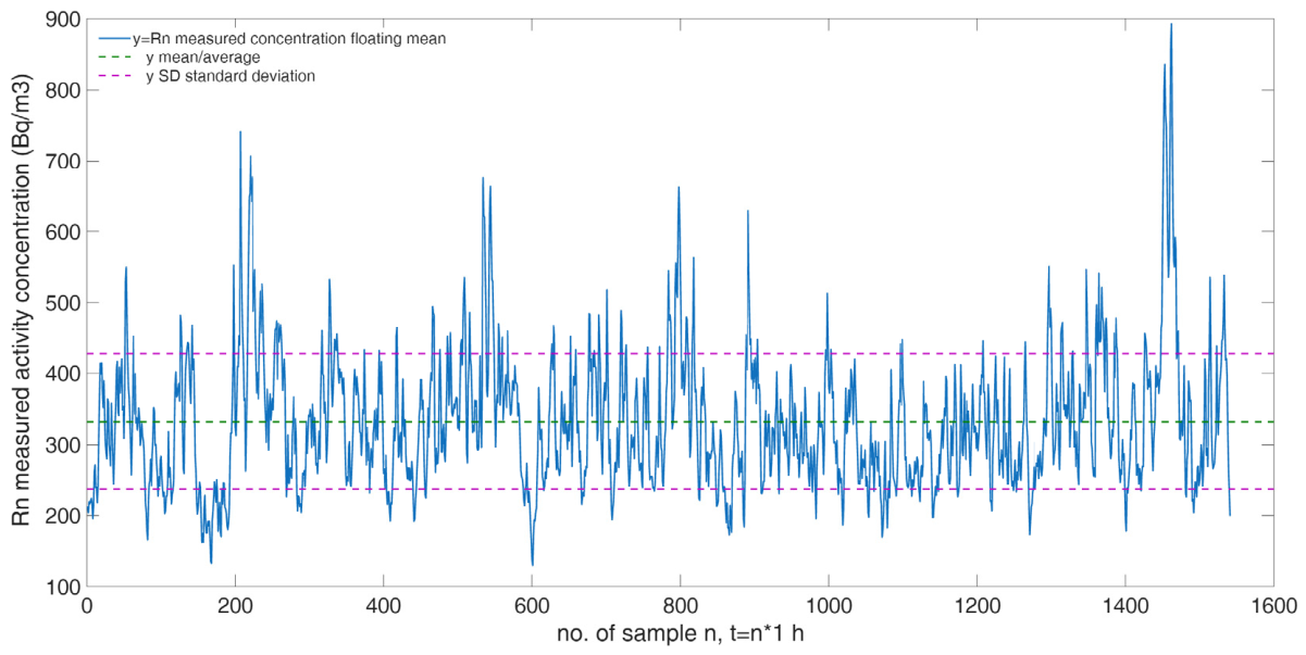
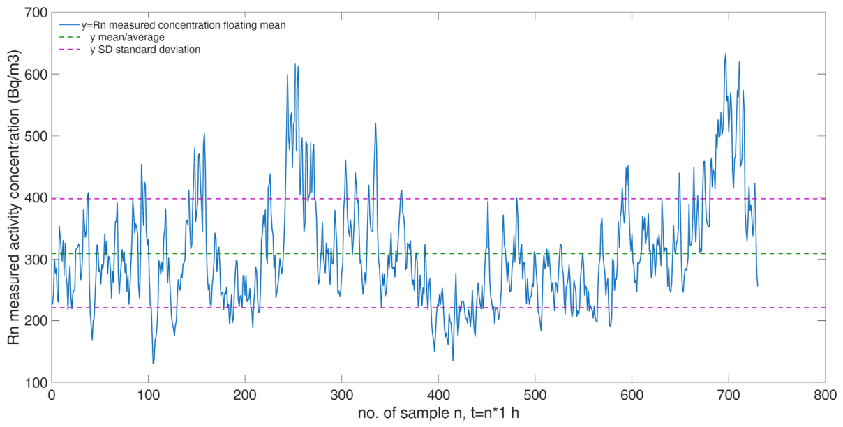
Note that in the presented graphs of measurements, axis x represents discrete values of sample no. n with 1 h time interval between any two samples n and n + 1, and axis y represents Rn measured concentrations in Bq/m³. The suggested national reference value in the EU for the annual average activity of Rn in air is 300 Bq/m³ [49,50,51], and the means of Rn concentration measurement results in both measurements are close to and higher than 300 Bq/m³. So, relevant short-term samples and their calculated means must be higher than 300 Bq/m³.

3.1.1. Measurement Results No.1

Measurement No.1 was performed within one corridor inside the St. Barbara mine with a natural geological environment, with some ventilation and very stable atmospheric/meteorological conditions. The basic parameters and results are presented in

Table 1. Parameters for measurement No.1.

Measurement ID	240709_024
Location	Corridor in St. Barbara mine
Instrument	Bertin AlphaE AE1
Duration of measurement	64.85 days/1556.5 h

and Figure 1.

3.1.2. Measurement Results No.2

Measurement No.2 was performed inside a small ground-floor room at UNIZG-FMGPE with minimal ventilation. The basic parameters and results are presented in

Table 2. Parameters for measurement No.2.

Measurement ID	2411-2501_025
Location	UNIZG-FMGPE building, basement, spectroscopy lab
Instrument	Bertin AlphaE AE1
Duration of measurement	30.46 days/731 h

and Figure 2.

3.2. Rn Measurement Signal Multiresolution Decomposition

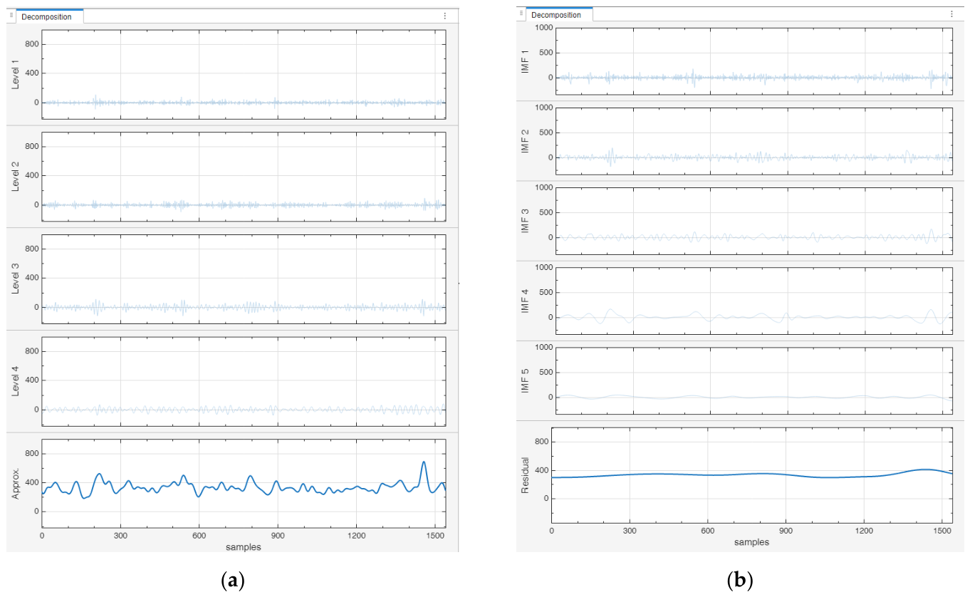
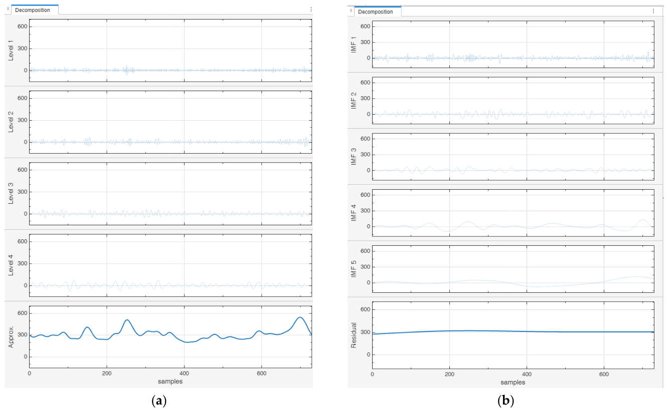
The Rn measurement signal was analyzed with MATLAB Signal decomposition–multiresolution analyzer with MODWT (maximal overlap discrete wavelet transform) method [28] and EMD (empirical mode decomposition) method [29]. Multiresolution analysis means decomposition of a signal into components, which, added together, make exactly the original signal. MODWT uses the Daubechies least-asymmetric wavelet and periodic boundary handling and returns the maximal overlap discrete wavelet transform. EMD is used to simplify complicated signals into a finite number of intrinsic mode functions required to perform Hilbert spectral analysis.

The Rn signal is composed of several components, of which one component is dominant (contains more than 90% of relative signal energy), and this component contains the Rn base concentration, which is due to the generation, entry and accumulation of Rn in a well-enclosed space and which converges to a finite, constant value of concentration with a variable part, which is due to changes in ambient meteorological parameters, ventilation, changes in Rn exhalation and entry rates (e.g., due to rainfall) and Rn migration.

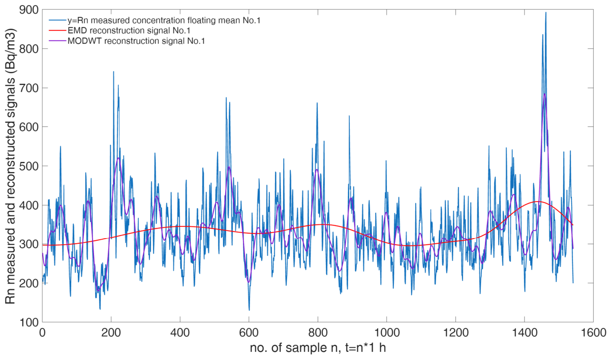
The results are presented for measurement No.1 in Figure 3 and Figure 4:

• MODWT method > 96% with frequency 0 h⁻¹ to 0.0311 h⁻¹ reconstructed signal.
• EMD method > 93% with frequency 0 h⁻¹ to 0.0311 h⁻¹ reconstructed signal.

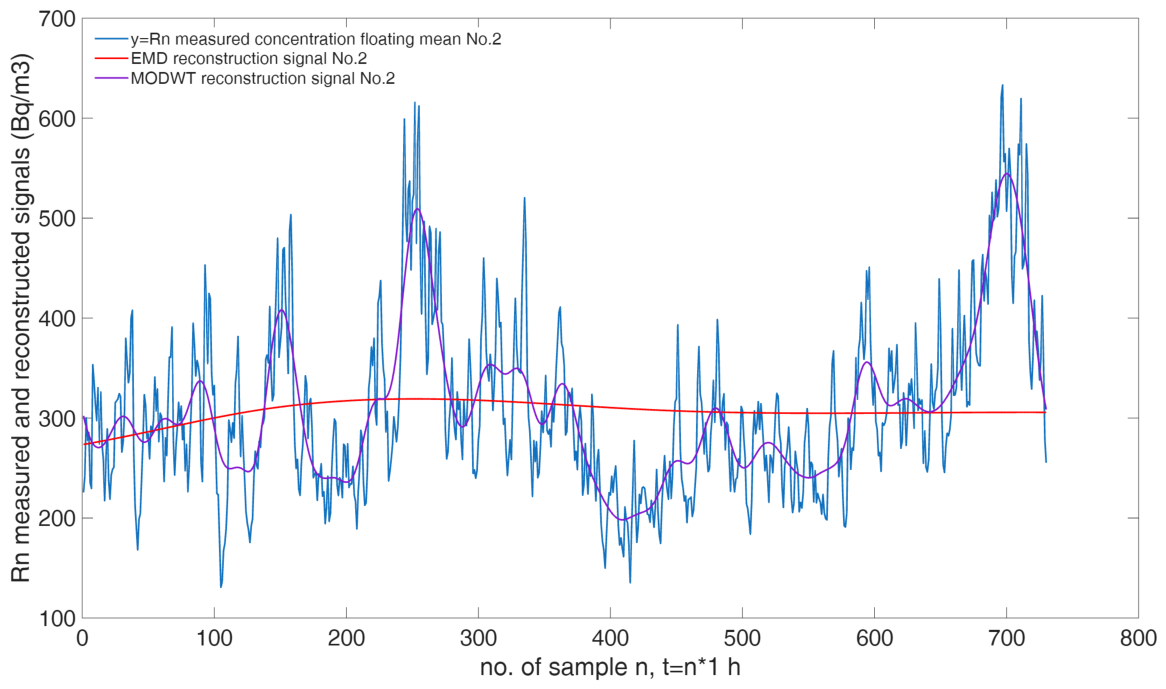
The MATLAB Signal decomposition–multiresolution analyzer results for measurement No.2 are presented in Figure 5 and Figure 6:

• MODWT method > 97% with frequency 0 h⁻¹ to 0.0311 h⁻¹ reconstructed signal No.2.
• EMD method > 92% with frequency 0 h⁻¹ to 0.0311 h⁻¹ reconstructed signal No.2.

Reconstructed signals have almost same mean as original signals. To estimate the variable part of the signal, the signal mean can be removed. This leaves the variable part of the signal, which has a mean close to 0, and this part is no longer relevant for estimating the mean. The variable part, however, shows Rn concentration changes due to changes in atmospheric parameters and precipitation, which is valuable for estimating how much these parameters influence changes from Rn base concentrations and give maximums of Rn concentrations, so this part will be estimated further.

The mean of the Rn concentration measurements of the whole dataset, in closed space without ventilation, is assumed to converge to a constant value because of the accumulation balance rule, as shown in Equation (1). For not entirely closed spaces, as in the presented measurements, the mean dataset will be the moving average, which is the goal of estimation and prediction. Convergence to the Rn balance concentration to constant value/process of Rn saturation can be expressed as in Equation (2):

$$f(x)=a·(1-e^{-b·x})$$

(2)

where:

• x = discrete t = i × 1 h, i = 0, 1, …, n, n >> 1, n = number of observations in dataset
• a = estimated stable and constant Rn concentration
• b (Rn half-decay constant λ_Rn1/2) = 0.00755 h⁻¹

In one year, 365 days, x = 8760 h, f(x) = 0.99999999999999999999999999998109 × a.

For short-term measurement (1 day, 2 days, 4 days and 8 days or 24 h, 48 h, 96 h and 192 h), which can be taken as a good observation/measurement sample set and first estimate of the mean, the probability that the mean of m-days observed dataset is below the mean value Rn_avg1 = 332.1 Bq/m³, which is the approximate reference value of 300 Bq/m³, as given in

Table 3. Probability that mean in datasets of 1,2,4 and 8 days is below 300 Bq/m³.

Days	No. Total	No. < Rnavg1	Probability from Histogram Distribution (%)
1	65	20	30.77
2	33	10	30.30
4	17	2	11.77
8	9	0	0

:

It can be observed that the longer the short-term measurement is, the higher the probability that the observation/measurement sample set is relevant; the difference in the daily and whole dataset mean concentration is also smaller. It follows that 1-day and 2-day measurements are too short, with approximately one in three samples not good. For 4-day measurements, it is very probable (almost 90%) that any 4-day sample will be representative and is good for the first estimate. For 8-day measurements, it is almost certain that any 8-day sample will be representative and is good for the first estimate. Consequently, the minimum time for measurements is 4 days/96 h or 8 days/192 h, with minimum 96 or 192 observations, each in 1 h.

3.3. Model Estimation Results

In the following sections, a number of models were estimated and validated, including linear regression with delays, transfer function, ARX, ARMAX and NLarx.

3.3.1. Linear Least Squares

The first model for estimation was linear regression for inputs indoor air temperature, pressure and humidity, estimating linear coefficients a₁, a₂, a₃ and time delays for inputs T_T, T_p, T_H, respectively, for indoor air temperature, inverse of air pressure (radon concentration is inversely influenced by air pressure) and relative humidity in vector x = [a₁ a₂ a₃ T_T T_p T_H]⁻¹, so that the Rn concentration is estimated in Equation (3):

$${Rn}_{est}=a_1·T_{temp°\mathrm{C}}(t-T_T)+{\displaystyle \frac{a_2}{p_{mbar}(t-Tp)}}+a_3·H_{rel}(t-T_H)$$

(3)

with the use of MATLAB functions optimset and fminsearch on two different whole datasets. The results are presented in

Table 4. Results of linear regression as model estimation.

dataset1 for Measurement No.1	dataset2 for Measurement No.2
a1 = 11.6784	a1 = 10.3700
a2 = 7.8206	a2 = 8.7373
a3 = 9.4523	a3 = 8.0818
TT = −0.0556	TT = −0.0489
Tp = 0.0069	Tp = 0.0069
TH = −0.0451	TH = −0.0486

, showing that the time delays of indoor air temperature, pressure and humidity are close to 0, meaning that these parameters have near-immediate effects on the change in the Rn concentration.

3.3.2. System Identification by Estimation and Validation

In the following estimations, the Rn concentration (Bq/m³) was smoothed with MATLAB Data Cleaner app/Smooth data/Moving mean.

Two options were estimated for measurements No.1 and No.2:

• Whole dataset of 1541 measurements/observations in measurement No.1 and 730 measurements/observations in measurement No.2.
• Whole dataset is divided into two sets, first for estimation of model and second for validation of model. Estimation set contains 8-day by 24 h = 192 measurements/observations. Validation set contains remainder of dataset. In measurement No.1, this was 1350 measurements/observations.

The considered input parameters were indoor air pressure (mbar), temperature (°C), relative humidity (%), precipitation/rain (mm), each averaged by their 1 h mean value. The output was the variation in the Rn concentration (Bq/m³) of cleaned/smoothed dataset given in Equation (4):

$$y=Rnc-mean\left(Rnc\right)$$

(4)

It was shown that the best results of validation were only with air pressure (mbar) and precipitation/rain (mm) as input parameters.

3.3.3. Model Identification

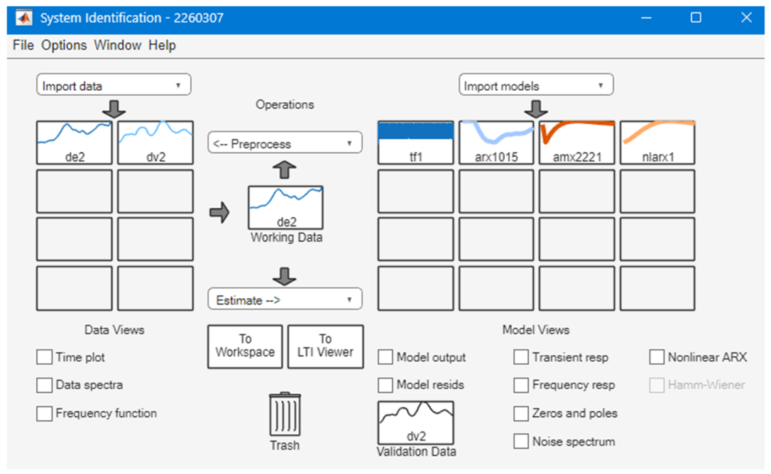
Models were estimated using the MATLAB System identification app, as presented in Figure 7.

The first step is to estimate different models on the whole dataset, to see which model gives usable results. Models used for prediction of the whole dataset were as follows: transfer function, polynomial models (ARX and ARMAX) [15,16] and non-linear merge of linear and statistical models NLARX [17,18].

Two model structures with relevant physical inputs as input variables were made with their mean value each 1 h, as shown in Supplementary File Table:

Four inputs u₁ = [p T H rain] and two inputs u₂ = [p rain], where:

• p—air pressure (mbar/hPa)
• T—air temperature (°C)
• H_rel—relative humidity (%)
• rain—rain/precipitation (mm)

Estimation and Validation for Measurement No.1

In

Table 5. Model estimation and validation results for the whole dataset No.1.

Model Identification	4 Input Parameters [p T H rain]	2 Input Parameters [p rain]
Transfer Function	tf3	tf2
Fit to estimation data	10.58%	27.11%
Fit to simulation	10.58	19
Fit to 1-step prediction	10.58	19
Polynomial ARX	arx1022	arx1031
Fit to estimation data	90.45%	91.9%
Fit to validation/simulation	16.02	14.26
Fit to 1-step prediction	90.45	29.28
Polynomial ARMAX	amx2221	amx2221
Fit to estimation data	88.99%	90.69%
Fit to validation/simulation	14.96	8.677
Fit to 1-step prediction	88.99	34.3
NLARX	nlarx1	nlarx4
Fit to estimation data	89.68%	91.07%
Fit to validation/simulation	24.26	15.31
Fit to 1-step prediction	89.68	39.11

, results are presented for the two structures (four and two parameters), with fit to estimation data in % and model output fit for simulation and one-step-ahead predicted output presented as Normalized Mean Squared Root Error (NMSRE cost function), which expresses the fit percentage using complement of the error norm for comparison and goodness-of-fit metric. The MATLAB compare function result of 100% or 100 is equivalent to a goodnessOfFit function result of 0.

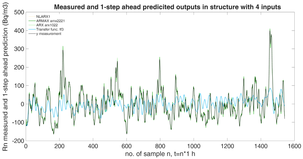
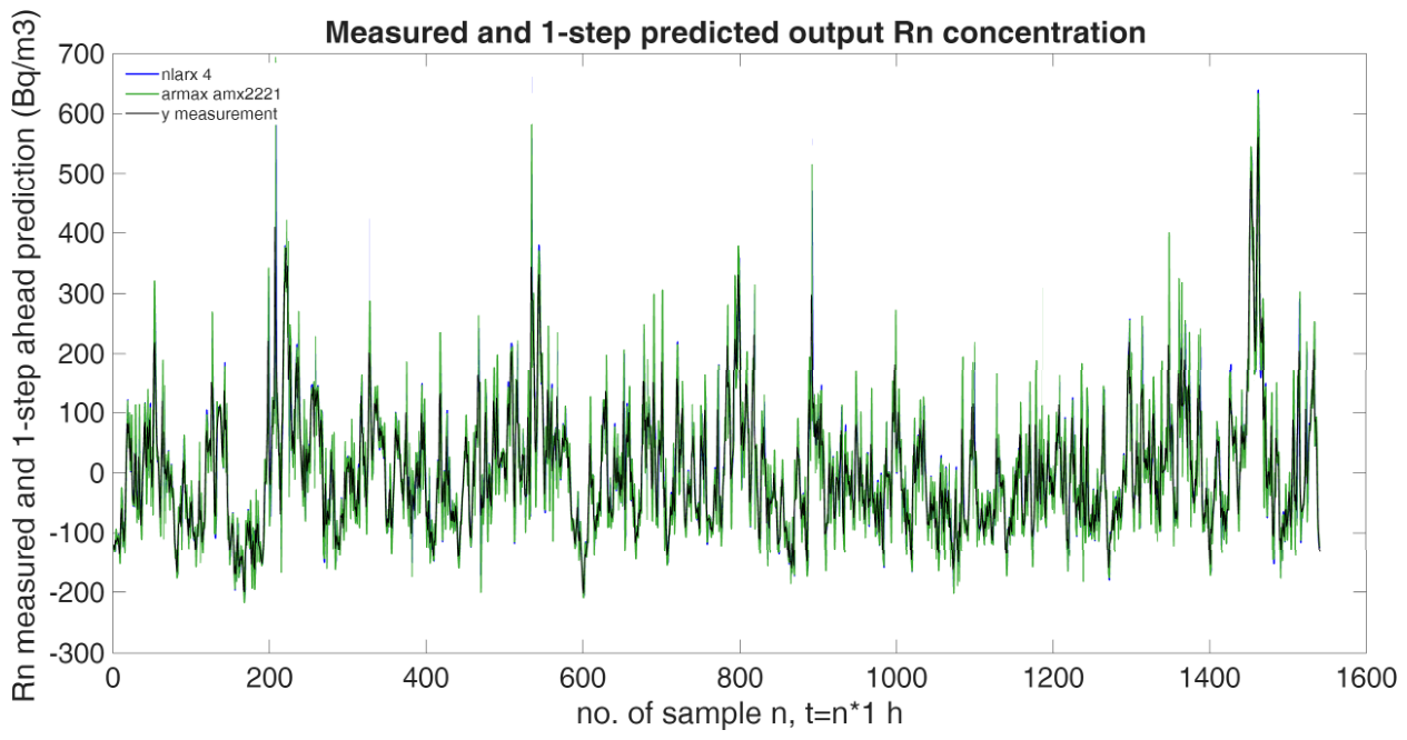
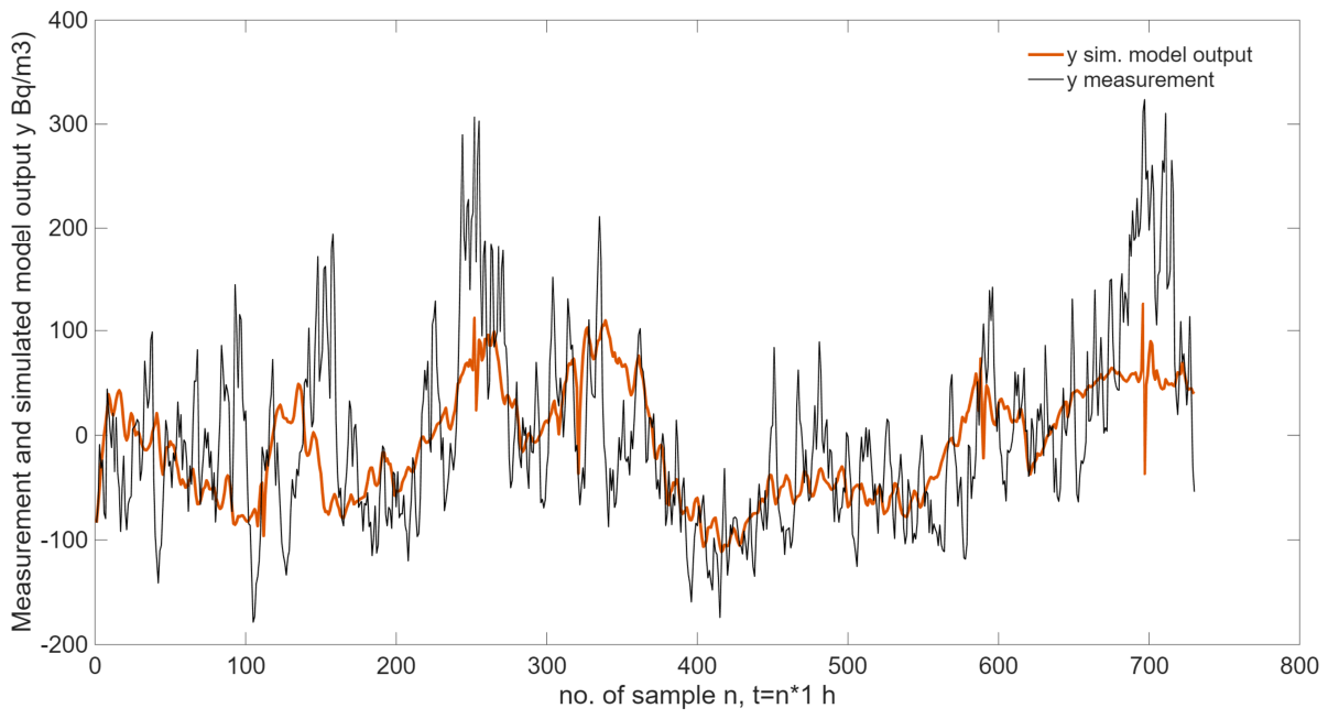
From the results shown in Table 5 and Figure 8 and Figure 9, it can be seen that the model structure with two inputs compared to the structure with four inputs gives similar results in simulation and acceptable results in one-step-ahead predicted output, so it was decided to check these two-input model estimations with partial datasets, a short one for estimation and longer one for validation of the models. Simulation output generally gave worse or poor results compared to one-step-ahead predicted output, so the latter was chosen as the preferred model output.

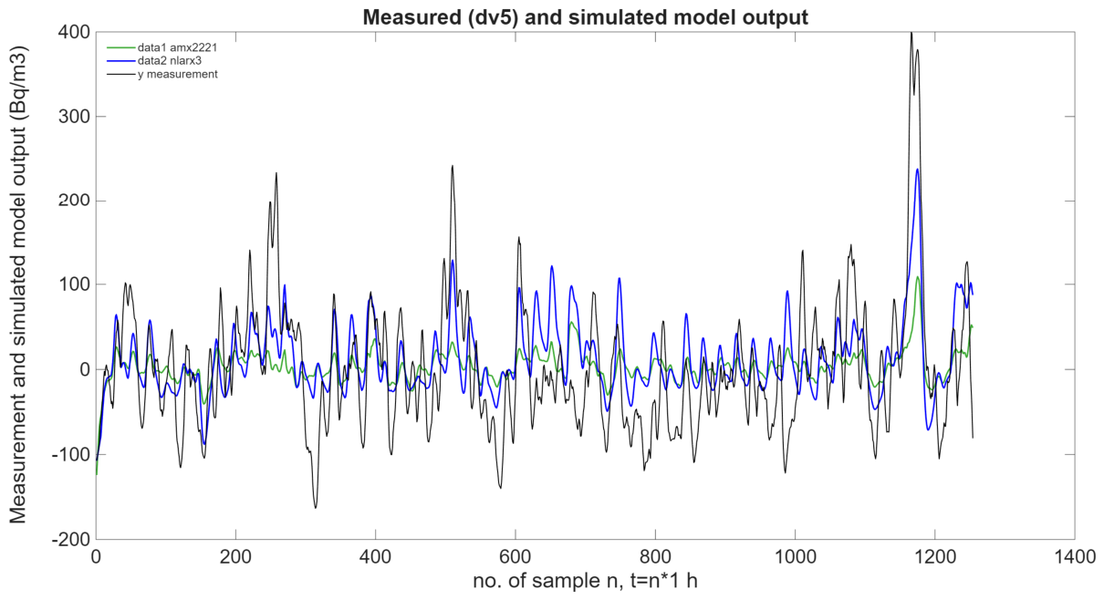
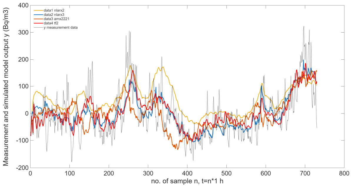
In the second step, two sets were created: 4-day and 8-day measurements/observations for estimation data. Both were checked, as shown in

Table 6. Results for dataset of 4 days: model, estimation and validation for Measurement No.1.

Model Identification	Fit to Estimation Data	NMSRE Fit to Validation Data
2 Input Parameters	Prediction Focus	(Simulation Output)/ (One-Step-Ahead Predicted Output)
Transfer Function
tf1	49.7%	−50.98/50.98
Polynomial ARX
arx1018	89.48%	18.78/89.24
Polynomial ARMAX
amx2221	87.4%	6.804/88.68
NLARX
nlarx1	100%	8.873/88.61

and

Table 7. Results for dataset of 8-days: model, estimation and validation for Measurement No.1.

Model Identification	Fit to Estimation Data	Fit to Validation Data
2 Input Parameters	Prediction Focus	(Simulation Output)/ (One-Step-Ahead Predicted Output)
Transfer Function
tf1	49.7%	−43.74/−43.74
Polynomial ARX
arx921	89.48%	20.43/89.73
Polynomial ARMAX
amx3332	90.75%	10.53/87.94
NLARX
nlarx3	93.46%	2.672/87.76

and Figure 10. The 4-day dataset in validation gave good results only for the NLarx model, so the minimum is to use 8-day measurements/observations for estimation data. The four (4)-input model had poor results with both ARMAX and NLarx validations, so it was dismissed as a good estimation model for short-term measurements.

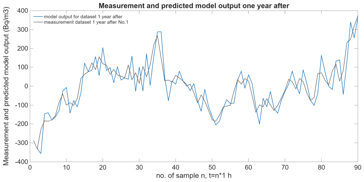
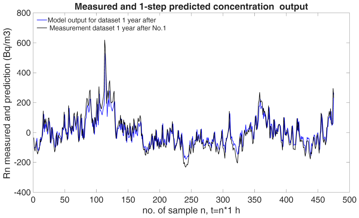
After this, a short measurement dataset of 90 h acquired one year after and at the exact same location as measurement No.1 was validated with the best model in one-step-ahead prediction (nlarx3), and this resulted as 46.75 NMSRE fit and R² = 0.7773, which is less than on the original dataset but still acceptable. This validation and fit are presented in Figure 11.

Estimation and Validation for Measurement No.2

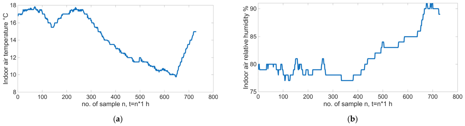
Indoor ambient parameters in measurement No.2 were specific due to air conditioning of the space, as shown in Figure 12, so part of the data was cut because air conditioning influences temperature and humidity (room is kept in specific micro-climate) but also brings force ventilation effects, which in these models are not considered, apart from natural air ventilation. Data cut out from the whole dataset were 1:250 and 650:end; after that time, the air conditioning remained off, and so the working dataset was 54.8% of the whole dataset. Eight-day estimation models, including the part when air conditioning is on, gave poor validation results.

In

Table 8. Model identification, estimation and validation results for the whole dataset No.2.

Model Identification	4 Input Parameters u = [p T H rain];	2 Input Parameters u2 = [p rain];
Transfer Function	tf2	tf1
Fit to estimation data	32.48%	15.05%
Fit to validation/simulation	32.48	15.05
Fit to 1-step prediction	32.48	15.05
Polynomial ARX	arx10105	arx10105
Fit to estimation data	58.15%	56.67%
Fit to validation/simulation	26.66	5.015
Fit to 1-step prediction	58.15	56.67
Polynomial ARMAX	amx2221	amx3332
Fit to estimation data	54.21%	50.15%
Fit to validation/simulation	11.12	−6.881
Fit to 1-step prediction	54.21	50.15
NLARX	nlarx3	nlarx4
Fit to estimation data	75.02%	55.69%
Fit to validation/simulation	33.02	20.17
Fit to 1-step prediction	75.02	55.69

, results are presented for the two structures (four and two input parameters) for measurements and models No.2. In

Table 9. Dataset of 8-day model estimation and validation results.

Model Identification	Fit to Estimation Data	Fit to Validation Data
2 Input Parameters	Prediction Focus	(Simulation Output)/ (One-Step-Ahead Predicted Output)
Transfer Function
tf1	42.65%	−18.89/−18.89
Polynomial ARX
arx116	57.31%	3.634/41.42
Polynomial ARMAX
amx3332	−181.9%	−406.8/−385
NLARX
nlarx4	64.95%	7.471/41.56

and Figure 13 and Figure 14, validation for the 8-day datasets is presented.

After this, a short measurement dataset of 475 h acquired one year after and at the exact same location as measurement No.2 was validated with the best model in one-step-ahead prediction (nlarx3), and this resulted as 51.27 NMSRE fit and R² = 0.7652, as shown in Figure 15.

Table 10. Comparison of prediction for datasets in Measurement No.1 and No.2 NRMSE fit.

Fit to Validation Data for 2-Input Models (NRMSE Fit Value) for One-Step-Ahead Predicted Output
NRMSE	Transfer Func.	ARX	ARMAX	NLARX
Measurement No.1
Whole dataset	27.11	91.9	90.69	80.16
4-day estimation	−50.98	89.24	88.68	88.61
8-day estimation	−43.74	89.73	87.94	87.76
12-day estimation	-	-	88.47	88.31
16-day estimation	-	-	88.63	88.47
Measurement No.2
Whole dataset	15.05	56.67	50.15	55.69
8-day estimation	−18.89	41.42	35.9 to 88.16	41.56 to 87.87
12-day estimation	-	-	88.76	88.97
16-day estimation	-	-	92.47	93.37

shows a comparison and summary of the results of one-step-ahead prediction for the two-input models for both locations and both measurements with the NRMSE fit value. The presented results show that the ARX model can give good prediction results, but its orders and delays change from dataset to dataset. ARMAX models are better in this regard but also show close changes in orders and delays and vary between polynomials of second and third order and delays of one and two samples. NLarx models are consistent in delays of 0 or 1 sample. It can be seen that some third-order ARMAX models may give a poor fit, as they show huge oscillations at the beginning of prediction, which was explained in previous research [26] as a natural period of oscillation, which is a characteristic of the dynamic systems. After that, prediction follows the measured reference much better. This can be corrected by changing the delay to 1 (1 h) for all inputs or reducing the model to second order. Overall, both ARMAX and NLarx may give very good fits with R² coefficients up to 0.99.

Also, prediction from estimation with the 8-day dataset gives similar results as prediction from estimation with bigger datasets of 12 days, 16 days or 30 days, as shown in Table 10 and

Table 11. Comparison of prediction for datasets in Measurement No.1 and No.2 R² coefficient.

Fit to Validation Data for 2 Inputs Models for One-Step-Ahead Predicted Output Correlation
R2	ARMAX	NLARX
Measurement No.1
Whole dataset	0.9913	0.9744
4-day estimation	0.9874	0.9874
8-day estimation	0.9871	0.9864
12-day estimation	0.9856	0.9850
16-day estimation	0.9870	0.9876
Measurement No.2
Whole dataset	0.7259	0.8027
8-day estimation	0.5898 to 0.9862	0.6627 to 0.9857
12-day estimation	0.9873	0.9878
16-day estimation	0.9941	0.9956

, with NRMSE fits and R² correlation coefficients. From this, it can be concluded that estimation from the 8-day dataset contains sufficient information to make “as good as it gets” prediction, and even 4-day estimation datasets are very similar in results. However, the sensitivity and dependency of which dataset is used for estimation, especially for 4-day datasets, needs to be established.

The next approach is to estimate models with a reconstructed Rn signal, as shown in Section 3.2. The MODWT reconstructed signal contains more than 95% of signal energy, and the EMD reconstructed signal contains more than 90% of signal energy; their mean is almost the same as the original measurement signal, and their forms are simpler than the original measurement dataset.

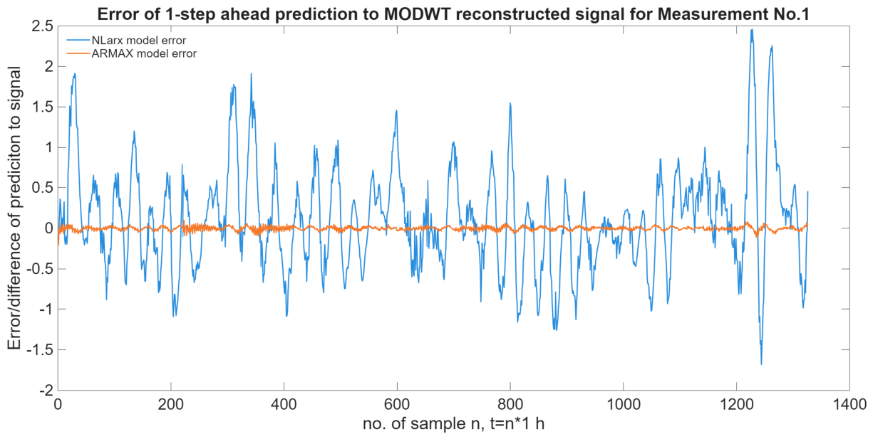
From the results of estimation of the MODWT reconstructed signal, neither model gives consistently good results in simulation output, as shown in

Table 12. Dataset estimation of 8 days for measurement No.1 with MODWT.

Model Identification	Fit to Estimation Data	Fit to Validation Data
2 Input Parameters	Prediction Focus	(Simulation Output)/ (One-Step-Ahead Prediction)
Transfer Function
tf2	27.98%	−335.8/−335.8
Polynomial ARX
arx916	99.96%	−58.29/99.99
Polynomial ARMAX
amx3332	99.9%	−64.16/99.96
NLARX
nlarx1	99.75%	−517.2/99.07

, but both ARMAX and NLarx give accurate results in one-step-ahead prediction output from 8-day short-term measurements. Therefore, only one-step-ahead prediction model output will be considered, and MODWT reconstructed signal prediction and ARMAX third-order polynomial and NLarx give accurate predictions with very small errors, as presented in Figure 16.

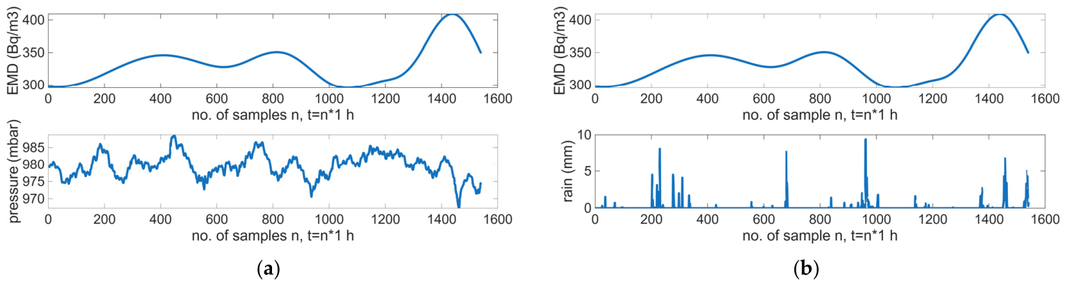
The next step was to estimate the EMD reconstruction signal with a simple polynomial ARMAX model to find out whether the simpler model polynomial of first order gives accurate prediction, as shown in Figure 17.

Correlations with air pressure and rain are shown in EMD reconstruction as y₁ and air pressure (u₁) and rain (u₂):

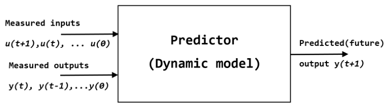
The one-step-ahead prediction model is presented in Figure 18.

Output of the one-step-ahead prediction y_p of the model y(t) + a ∙ y(t − 1) = b ∙ u(t) is given in Equation (5):

y_p(t + 1) = −a ∙ y_p(t) + b ∙ u(t + 1)

(5)

In this simple one-step case for the predicted output for t + 1, the newest prediction is based only on measurements of inputs for t + 1 and previously predicted output for t.

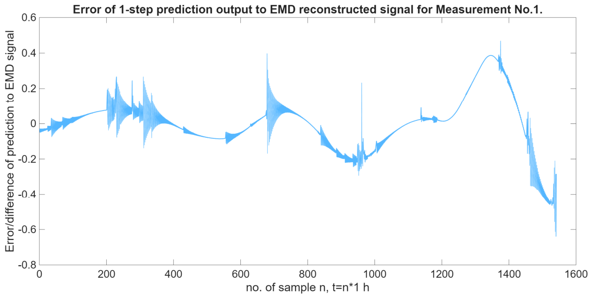
The whole EMD reconstruction signal for measurement No.1 is successfully estimated with ARMAX with one-step-ahead predicted output, and the fit to estimation data is 99.46% (prediction focus), as shown in Figure 19. The discrete-time ARMAX model is given by a set of equations for A(z), B(z) and C(z) polynomials, with coefficients presented in Table 13.

Table 13. Dataset estimation of 8 days for measurement No.2 with MODWT reconstructed signal.

Model Identification	Fit to Estimation Data	Fit to Validation Data
2 Input Parameters	Prediction Focus	(Simulation Output)/ (One-Step-Ahead Prediction)
Transfer Function
tf2	61.52%	−30.78/−30.78
Polynomial ARX
arx916	95.48%	n/a/n/a
Polynomial ARMAX
amx3332	99.98%	−105.6/99.96
NLARX
nlarx3	99.71%	21.38/99.34

Table 13. Dataset estimation of 8 days for measurement No.2 with MODWT reconstructed signal.

Model Identification	Fit to Estimation Data	Fit to Validation Data
2 Input Parameters	Prediction Focus	(Simulation Output)/ (One-Step-Ahead Prediction)
Transfer Function
tf2	61.52%	−30.78/−30.78
Polynomial ARX
arx916	95.48%	n/a/n/a
Polynomial ARMAX
amx3332	99.98%	−105.6/99.96
NLARX
nlarx3	99.71%	21.38/99.34

Figure 19. Error of 1-step prediction output to EMD reconstructed signal for measurement No.1.

Figure 19. Error of 1-step prediction output to EMD reconstructed signal for measurement No.1.

The EMD reconstruction signal for measurement No.2 is successfully estimated with ARMAX.

The discrete-time ARMAX model is given by a set of equations for A(z), B(z) and C(z) polynomials, as shown in

Table 14. ARMAX model polynomial equations and coefficients for EMD signal in No.1.

$A\left(z\right)·y\left(t\right)=B\left(z\right)·u\left(t\right)+C\left(z\right)·e\left(t\right)$

$A\left(z\right)=1-0.9993·z^{-1}$

$B_1\left(z\right)=0.0002918·z^{-1}$

$B_2\left(z\right)=-0.04049·z^{-1}$

$C\left(z\right)=1+0.9558·z^{-1}$

:

From this, it can be seen that the ARMAX model gives an excellent description of the EMD reconstruction signal in one-step lead predicted output when the whole signal dataset is estimated, and A(z) and C(z) polynomial parts are almost the same in both measurements, while B₁(z) and B₂(z) have similar parameters, so A(z), B(z) and C(z) polynomial parts can be approximated to the polynomials shown in

Table 15. ARMAX model polynomial equations and coefficients for EMD signal in No.2.

$A\left(z\right)·y\left(t\right)=B\left(z\right)·u\left(t\right)+C\left(z\right)·e\left(t\right)$

$A\left(z\right)=1-0.986·z^{-1}$

$B_1\left(z\right)=0.004302·z^{-1}$

$B_2\left(z\right)=0.03651·z^{-1}$

$C\left(z\right)=1+0.99·z^{-1}$

:

Where B1(z) is linked to input No.1 (air pressure) and B2(z) is linked to input No.2 (rain).

Since this was checked only for two locations and two measurement datasets shown as approximation in

Table 16. ARMAX model polynomial equations and approximate coefficients for EMD.

$A\left(z\right)=1-1·z^{-1}$

$B_1\left(z\right)=0.004·z^{-1}$

$B_2\left(z\right)=0.04·z^{-1}$

$C\left(z\right)=1+1·z^{-1}$

, this is only an indication of the working model for other locations and datasets. This would have to be researched further to provide confidence intervals for the estimated coefficients and the range within which the B1 and B2 parameters may vary for other types of rooms and geological conditions, as well as how such variability would affect the accuracy of mean prediction.

This shows that ARMAX in one-step lead predicted output may be an excellent model for estimating EMD reconstruction, which has almost the same mean as the original signal, i.e., it can potentially be used generally for the prediction of the Rn mean, its accuracy depending on the estimated parameters of B polynomials. EMD has a simpler form as MODWT, and its form is very easily described by a first-order polynomial with very similar coefficients in one-step-ahead prediction. For MODWT, a third-order polynomial is needed with changing coefficients. EMD seems to retain the slow trend of radon concentration, which is not in the scope of this study.

4. Conclusions

MATLAB and modelling for the prediction of radon have been used in previous research, e.g., ARMAX models, and are still being researched. This work extends to non-linear methods such as NLarx and provides comparative analysis of four prediction model identifications and two structures on datasets of different time length/size. Reconstruction/decomposition signal methods and the simple ARMAX model of this signal indicate a relation to the seasonal mean. The model with only two meteorological parameters shows similar results to the more complex model with four parameters. According to the results of this research, 8-day short-term measurements may be a good indication for the Rn concentration variation in a season and an indication of the seasonal mean value. Datasets from measurements one year after the first ones at the same location and in the same season were validated using previously identified models, and NLarx model performance seems to be good.

The key limitations of this research include the following:

• Measurements performed and compared for only two micro-locations.
• Relatively short absolute duration of validation to the annual cycle being predicted, so only change for one season is considered.
• Seismic parameter as input is not considered in this study.
• Ventilation effect as input is not considered in this study. We researched closed systems without much ventilation, because they have much more probability of radon accumulation and higher levels.
• Dependency and sensitivity of all models’ performances to estimation dataset selection, i.e., which samples from whole measurement are selected for estimation dataset.

Future research directions may include the following:

• Complete annual and seasonal measurements and estimation of annual model.
• Validation of prediction model at more locations and micro-locations.
• Identifying micro-locations where the radon mean is close to the recommended level.
• Adding seismic and/or geology parameters to model inputs.
• Researching ventilation effects.
• Development and validation of models with statistical methods, neural networks, data-driven models and machine learning.
• Research and validation of modes on datasets from other research based on Europe-wide radon atlas.
• Build-up of standard database with radon datasets from locations.

MATLAB data analysis and system identification lead to the following conclusions:

The Rn concentration measurement signal is composed of several components, of which one component is dominant (contains more than 90% of relative signal energy), and this component contains the Rn base concentration, which converges to a finite, constant value, which is the Rn concentration mean with variable part.

The dominant component of signal EMD reconstruction for Rn measurement signal decomposition has almost the same mean as the original signal, and its ARMAX one-step predicted output model can be approximated by simple first-order polynomials, which give excellent estimation and validation of the EMD reconstruction signal. This one-step predicted output of the simple first-order polynomial ARMAX model gives a very good estimation of the Rn mean.

System identification of the variable part from short-term measurements can be reduced to 8-day measurements with only two input parameters, air pressure and rain. Four-day short measurements may give good predictions, and longer than 8-day datasets give similar results to datasets of 8 days. Dependency on which samples from the whole measurement are selected for the estimation dataset needs to be further researched. This is in line with a previous study, showing that the measurement times for obtaining radon concentrations should not be less than 4 days.

The most consistent results for validation of the variable part are obtained by using NLarx model estimation. Other models can give good results and poor validation, depending on the short-term set of measurements selected for estimation. For a longer set of measurements for estimation, good results can be obtained with ARMAX, ARX and transfer function models.

From the validation results, the following can be concluded:

• Transfer models do not give good validation if estimation data are from short-term measurements (4 days or 8 days).
• Polynomial ARX models can give good results, but their polynomial order structure and delays change from case to case.
• Polynomial ARMAX models in one location give very good results, especially second- and third-order model structure, but not in other locations.
• NLarx models give consistently good results, so they are the preferred estimation model to predict Rn concentration variations from short-term measurements of 8 days.
• For validation from short-term estimations of 8 days, two-input models give similar results to four-input models.
• The one-step predicted output ARMAX model gives excellent estimation of MODWT and EMD reconstructed signals, which has approximately the same mean as the original signal, i.e., can be used for prediction of the Rn mean. The EMD signal ARMAX model is a very simple first-order polynomial and useful for indirect prediction of the Rn mean from the EMD reconstructed signal.
• Since the NLarx model showed very good results in the validation of Rn concentration variations for both the whole and part of datasets, i.e., longer and shorter than 8-day measurements/observations, this model is selected as the preferred model.

References

1. LNE-LNHB/CEA- Atomic and Nuclear Data. Available online: http://www.lnhb.fr/home/nuclear-data/nuclear-data-table/ (accessed on 23 June 2026).
2. Isotopes of Radon—Periodic Table. Available online: https://pse-info.de/en/isotopes/Rn (accessed on 24 March 2026).
3. Radon (Rn) Isotopes|ChemReference Periodic Table. Available online: https://chemreference.com/periodic-table/radon/isotopes (accessed on 24 March 2026).
4. Gugliermetti, L.; Lepore, L.; Remetti, R.; Tosti, M.C. Alpha spectrometry with the inexpensive open-source detector Alphaino. Nucl. Instrum. Methods Phys. Res. A 2019, 928, 13–19. [Google Scholar] [CrossRef]
5. Sofia Clareu Elísio, S.; Luís Peralta, D. Development of an Active Detector for Radon Detection in Air. 2019. Available online: https://repositorio.ulisboa.pt/handle/10451/39062 (accessed on 16 June 2025).
6. Voytchev, M.; Klein, D.; Chambaudet, A.; Georgiev, G.; Iovtchev, M. Applications of a silicon photodiode detector for radon progeny measurements. Radiat. Meas. 1999, 31, 375–378. [Google Scholar] [CrossRef]
7. Gutiérrez, J.L.; García-Talavera, M.; Peña, V.; Nalda, J.C.; Voytchev, M.; López, R. Radon emanation measurements using silicon photodiode detectors. Appl. Radiat. Isot. 2004, 60, 583–587. [Google Scholar] [CrossRef] [PubMed]
8. Development of an Active Alpha Particle Detector for Radon and Its Daughter Products. Available online: https://www.researchgate.net/publication/387534934_DEVELOPMENT_OF_AN_ACTIVE_ALPHA_PARTICLE_DETECTOR_FOR_RADON_AND_ITS_DAUGHTER_PRODUCTS (accessed on 24 March 2026).
9. Chambaudet, A.; Klein, D.; Voytchev, M. Study of the response of silicon detectors for alpha particles. Radiat. Meas. 1997, 28, 127–132. [Google Scholar] [CrossRef]
10. ISO 11665-7:2012(en); Measurement of Radioactivity in the Environment—Air: Radon-222—Part 7: Accumulation Method for Estimating Surface Exhalation Rate. ISO: Geneva, Switzerland, 2012. Available online: https://www.iso.org/obp/ui/en/#iso:std:iso:11665:-7:ed-1:v1:en (accessed on 20 March 2025).
11. Font, G.L. Radon Generation, Entry and Accumulation Indoors; Universitat Autònoma de Barcelona: Barcelona, Spain, 1997. [Google Scholar]
12. Font, L.; Baixeras, C. The RAGENA dynamic model of radon generation, entry and accumulation indoors. Sci. Total Environ. 2003, 307, 55–69. [Google Scholar] [CrossRef] [PubMed]
13. Font, L.L.; Baixeras, C.; Domingo, C.; Fernandez, F. Experimental and theoretical study of radon levels and entry mechanisms in a mediterranean climate house. Radiat. Meas. 1999, 31, 277–282. [Google Scholar] [CrossRef]
14. Nunes, L.J.R.; Curado, A.F.; Lopes, S.E.I. The Relationship between Radon and Geology: Sources, Transport and Indoor Accumulation. Appl. Sci. 2023, 13, 7460. [Google Scholar] [CrossRef]
15. Florică, Ş.; Burghele, B.D.; Bican-Brişan, N.; Begy, R.; Codrea, V.; Cucoş, A.; Catalina, T.; Dicu, T.; Dobrei, G.; Istrate, A.; et al. The path from geology to indoor radon. Environ. Geochem. Health 2020, 42, 2655–2665. [Google Scholar] [CrossRef] [PubMed]
16. Mostečak, A.; Perković, D.; Kapor, F.; Veinović, Ž. Radon mapping in Croatia and its relation to geology. Rud.-Geološko-Naft. Zb. 2018, 33, 1–11. [Google Scholar] [CrossRef]
17. Gillmore, G.K.; Phillips, P.S.; Denman, A.R. The effects of geology and the impact of seasonal correction factors on indoor radon levels: A case study approach. J. Environ. Radioact. 2005, 84, 469–479. [Google Scholar] [CrossRef] [PubMed]
18. Robinson, A.L.; Sextro, R.G. Radon entry into buildings driven by atmospheric pressure fluctuations. Environ. Sci. Technol. 1997, 31, 1742–1748. [Google Scholar] [CrossRef]
19. Kitto, M.E. Interrelationship of indoor radon concentrations, soil-gas flux, and meteorological parameters. J. Radioanal. Nucl. Chem. 2005, 264, 381–385. [Google Scholar] [CrossRef]
20. Janik, M.; Łoskiewicz, J.; Tokonami, S.; Kozak, K.; Mazur, J.; Ishikawa, T. Determination of the minimum measurement time for estimating long-term mean radon concentration. Radiat. Prot. Dosim. 2012, 152, 168–173. [Google Scholar] [CrossRef] [PubMed]
21. Siino, M.; Scudero, S.; D’Alessandro, A. Stochastic Models for Radon Daily Time Series: Seasonality, Stationarity, and Long-Range Dependence Detection. Front. Earth Sci. 2020, 8, 462. [Google Scholar] [CrossRef]
22. Mose, D.G.; Mushrush, G.W.; Chrosniak, C.E.; Morgan, W.F. Seasonal indoor radon variations related to precipitation. Environ. Mol. Mutagen. 1991, 17, 223–230. [Google Scholar] [CrossRef] [PubMed]
23. Krewski, D.; Mallick, R.; Zielinski, J.M.; Létourneau, E.G. Modeling seasonal variation in indoor radon concentrations. J. Expo. Anal. Environ. Epidemiol. 2005, 15, 234–243. [Google Scholar] [CrossRef] [PubMed]
24. Pinel, J.; Fearn, T.; Darby, S.C.; Miles, J.C.H. Seasonal Correction Factors for Indoor Radon Measurements in the United Kingdom. Radiat. Prot. Dosim. 1995, 58, 127–132. [Google Scholar] [CrossRef]
25. Arvela, H. Seasonal variation in radon concentration of 3000 dwellings with model comparisons. Radiat. Prot. Dosim. 1995, 59, 33–42. [Google Scholar] [CrossRef]
26. Pepperosa, A.; Remetti, R.; Perondi, F. ARMAX Forecast Model for Estimating the Annual radon Activity Concentration in Confined Environment by Short Measurements Performed by Active Detectors. Int. J. Environ. Res. Public Health 2022, 19, 5229. [Google Scholar] [CrossRef] [PubMed]
27. Barros, N.G.; Steck, D.J.; Field, R.W. A comparison of winter short-term and annual average radon measurements in basements of a radon-prone region and evaluation of further radon testing indicators. Health Phys. 2014, 106, 535–544. [Google Scholar] [CrossRef] [PubMed]
28. Modwt-Maximal Overlap Discrete Wavelet Transform-MATLAB. Available online: https://uk.mathworks.com/help/wavelet/ref/modwt.html (accessed on 25 March 2026).
29. Emd-Empirical Mode Decomposition-MATLAB. Available online: https://uk.mathworks.com/help/signal/ref/emd.html (accessed on 25 March 2026).
30. Rey, J.F.; Goyette, S.; Goyette Pernot, J. Weather Impacts on Indoor Radon Short-Term Measurements in Switzerland. Atmosphere 2023, 14, 1163. [Google Scholar] [CrossRef]
31. Dvorzhak, A.; Mora, J.C.; Real, A.; Sainz, C.; Fuente, I. General model for estimation of indoor radon concentration dynamics. Environ. Sci. Pollut. Res. 2021, 28, 54085–54095. [Google Scholar] [CrossRef] [PubMed]
32. Groves-Kirkby, C.J.; Crockett, R.G.M.; Denman, A.R.; Phillips, P.S. A critical analysis of climatic influences on indoor radon concentrations: Implications for seasonal correction. J. Environ. Radioact. 2015, 148, 16–26. [Google Scholar] [CrossRef] [PubMed]
33. AlphaE-Ultra-Small Radon Monitor-Bertin Technologies. Available online: https://www.bertin-technologies.com/product/radon-professional-monitoring/radon-alphae/ (accessed on 24 March 2026).
34. Mphaga, K.V.; Mbonane, T.P.; Utembe, W.; Rathebe, P.C. Short-Term vs. Long-Term: A Critical Review of Indoor Radon Measurement Techniques. Sensors 2024, 24, 4575. [Google Scholar] [CrossRef] [PubMed]
35. Park, J.H.; Kang, D.R.; Kim, J. A review on mathematical models for estimating indoor radon concentrations. Ann. Occup. Environ. Med. 2016, 28, 7. [Google Scholar] [CrossRef] [PubMed]
36. Wei, W.; Ramalho, O.; Malingre, L.; Sivanantham, S.; Little, J.C.; Mandin, C. Machine learning and statistical models for predicting indoor air quality. Indoor Air 2019, 29, 704–726. [Google Scholar] [CrossRef] [PubMed]
37. Elío, J.; Petermann, E.; Bossew, P.; Janik, M. Machine learning in environmental radon science. Appl. Radiat. Isot. 2023, 194, 110684. [Google Scholar] [CrossRef] [PubMed]
38. Signal Multiresolution Analyzer-Decompose Signals into Time-Aligned Components-MATLAB. Available online: https://uk.mathworks.com/help/wavelet/ref/signalmultiresolutionanalyzer-app.html (accessed on 24 March 2026).
39. Tfest-Estimate Transfer Function Model-MATLAB. Available online: https://uk.mathworks.com/help/ident/ref/tfest.html (accessed on 24 March 2026).
40. Armax-Estimate Parameters of ARMAX, ARIMAX, ARMA, or ARIMA Model Using Time-Domain Data-MATLAB. Available online: https://uk.mathworks.com/help/ident/ref/armax.html (accessed on 18 March 2026).
41. Idnlarx-Nonlinear ARX Model-MATLAB. Available online: https://uk.mathworks.com/help/ident/ref/idnlarx.html (accessed on 18 March 2026).
42. Vukošić, H.; Ban, Ž.; Kuhinek, D.; Veinović, Ž. Examples of Comparative Measurements of Active Concentration of Radon (Rn) in Air in Croatia; University of Zagreb, Faculty of Mining, Geology and Petroleum Engineering: Zagreb, Croatia, 2025. [Google Scholar]
43. Radolić, V.; Vuković, B.; Stanić, D.; Katić, M.; Faj, Z.; Šuveljak, B.; Lukačević, I.; Faj, D.; Lukić, M.; Planinić, J. National survey of indoor radon levels in Croatia. J. Radioanal. Nucl. Chem. 2006, 269, 87–90. [Google Scholar] [CrossRef]
44. Siročić, A.P.; Stanko, D.; Sakač, N.; Dogančić, D.; Trojko, T. Short-Term Measurement of Indoor Radon Concentration in Northern Croatia. Appl. Sci. 2020, 10, 2341. [Google Scholar] [CrossRef]
45. Data Analysis–MATLAB & Simulink-MATLAB & Simulink. Available online: https://uk.mathworks.com/products/matlab/data-analysis.html (accessed on 24 March 2026).
46. Curve Fitter-Fit Curves and Surfaces to Data-MATLAB. Available online: https://uk.mathworks.com/help/curvefit/curvefitter-app.html (accessed on 24 March 2026).
47. Working with System Identification App-MATLAB & Simulink. Available online: https://uk.mathworks.com/help/ident/ug/working-with-the-system-identification-tool-gui.html (accessed on 24 March 2026).
48. Fminsearch-Search for Local Minimum of Unconstrained Multivariable Function Using Derivative-Free Method-MATLAB. Available online: https://uk.mathworks.com/help/matlab/ref/fminsearch.html (accessed on 24 March 2026).
49. Directive 2013/59/Euratom-Protection Against Ionising Radiation|Safety and Health at Work EU-OSHA. Available online: https://osha.europa.eu/en/legislation/directives/directive-2013-59-euratom-protection-against-ionising-radiation (accessed on 28 May 2025).
50. Radon|IAEA. Available online: https://www.iaea.org/topics/radiation-protection/radon (accessed on 28 May 2025).
51. WHO. WHO Handbook on Indoor Radon. Int. J. Environ. Stud. 2009, 67, 100–102. Available online: http://www.tandfonline.com/doi/abs/10.1080/00207230903556771 (accessed on 17 March 2025).
Figure 1. Rn floating mean 1 h results for measurement No.1.
Applsci 16 06625 g001
Figure 2. Rn floating mean 1 h results for measurement No.2.
Applsci 16 06625 g002
Figure 3. (a) MODWT and (b) EMD decomposition of measurement signal No.1.
Applsci 16 06625 g003
Figure 4. MODWT and EMD reconstruction signals and original measurement No.1.
Applsci 16 06625 g004
Figure 5. (a) MODWT and (b) EMD decomposition of measurement signal No.2.
Applsci 16 06625 g005
Figure 6. MODWT and EMD reconstruction signals and original measurement No.2.
Applsci 16 06625 g006
Figure 7. System identification app—estimation with 2 data structures.
Applsci 16 06625 g007
Figure 8. Measured and one-step-ahead predicted outputs in structure with 4 inputs.
Applsci 16 06625 g008
Figure 9. Measured and one-step-ahead predicted outputs in structure with 2 inputs.
Applsci 16 06625 g009
Figure 10. Dataset of 8 days with 2-input NLarx and ARMAX model outputs validation.
Applsci 16 06625 g010
Figure 11. Model output validation one year after measurement No.1 for 2-input NLarx.
Applsci 16 06625 g011
Figure 12. Indoor air temperature (a) and air rel. humidity; (b) time-series dataset in measurement No.2.
Applsci 16 06625 g012
Figure 13. Validation of NLarx model estimated from 8 days with 2-input NLarx model.
Applsci 16 06625 g013
Figure 14. Validation of 2 NLarx models estimated from 8 days with 4 inputs of the whole dataset.
Applsci 16 06625 g014
Figure 15. Model output validation one year after measurement No.2 for 2-input NLarx.
Applsci 16 06625 g015
Figure 16. Error of 1-step prediction output to MODWT reconstructed signal for measurement No.1.
Applsci 16 06625 g016
Figure 17. EMD reconstruction signal compared to 2 inputs: air pressure (a) and rain (b).
Applsci 16 06625 g017
Figure 18. Predict identified output model (1-step predictor dynamic model).
Applsci 16 06625 g018