A Boundary-Guided Feature Modulation Network for Weld Radiographic Defect Segmentation

Abstract

Accurate pixel-level segmentation of weld defects in radiographic images is essential for automated non-destructive testing (NDT) and quantitative weld-quality assessment. However, this task remains challenging because weld defects often exhibit severe foreground–background imbalance, ambiguous boundaries, weak grayscale contrast, and defect-like weld background structures, which can lead to boundary over-expansion and false-positive predictions. To address these issues, this paper proposes a boundary-guided feature modulation framework with false-positive suppression for weld radiographic defect segmentation. The method constructs boundary bands from training annotations and uses them only as label-derived training-time regularizers for attention-driven feature modulation and region-aware optimization; during validation and testing, no ground-truth mask, boundary band, or predicted boundary map is provided to the model. Multi-scale feature fusion is used to recover weak defect responses, boundary-guided dual attention enhances boundary-sensitive feature representation, and a false-positive suppression loss penalizes foreground leakage above a tolerated confidence margin in stable non-boundary background regions. Experiments on a real-world pipeline weld radiographic dataset containing 10,079 images show that the proposed method achieves a Dice score of $0.810\pm 0.003$, a Precision of $0.809\pm 0.004$, and a Surface Dice at 3 pixels of $0.394\pm 0.008$, outperforming representative CNN-based and Transformer-based segmentation baselines. Ablation studies, qualitative visualization, and distance-based false-positive analysis further demonstrate that the proposed framework improves contour reliability and reduces background false positives.

1. Introduction

Industrial weld radiographic inspection is widely used in non-destructive testing (NDT) to assess the internal quality of critical welded structures, such as pressure vessels and pipelines. Weld defects may reduce structural reliability, affect service safety, and increase the risk of leakage or failure. Therefore, accurate and efficient interpretation of weld radiographs is an important task in industrial quality inspection [1,2,3]. With the increasing demand for automated NDT, defect segmentation is not only an intermediate image-processing step, but also a key basis for downstream defect assessment. Compared with image-level classification or bounding-box detection, pixel-level segmentation can provide more detailed information, including defect area, contour, extent, and spatial distribution, which is essential for quantitative evaluation and inspector-assisted decision making.

In recent years, deep learning has been actively explored for weld radiographic analysis. Many studies have focused on defect classification, heat-map localization, or coarse detection [4,5,6,7], whereas relatively few studies have specifically addressed pixel-level segmentation of weld defects in radiographic images [8,9]. For weld radiographic inspection, pixel-level defect segmentation is more informative than classification or coarse localization, since it explicitly delineates the defective region rather than merely indicating its category or approximate position. This capability is crucial for radiographic defects with weak grayscale contrast, irregular morphology, and ambiguous boundaries, where bounding boxes or image-level labels are often insufficient to represent the true defect extent. Therefore, accurate defect segmentation can support quantitative defect size estimation, boundary measurement, false-positive reduction, and more reliable automated NDT workflows.

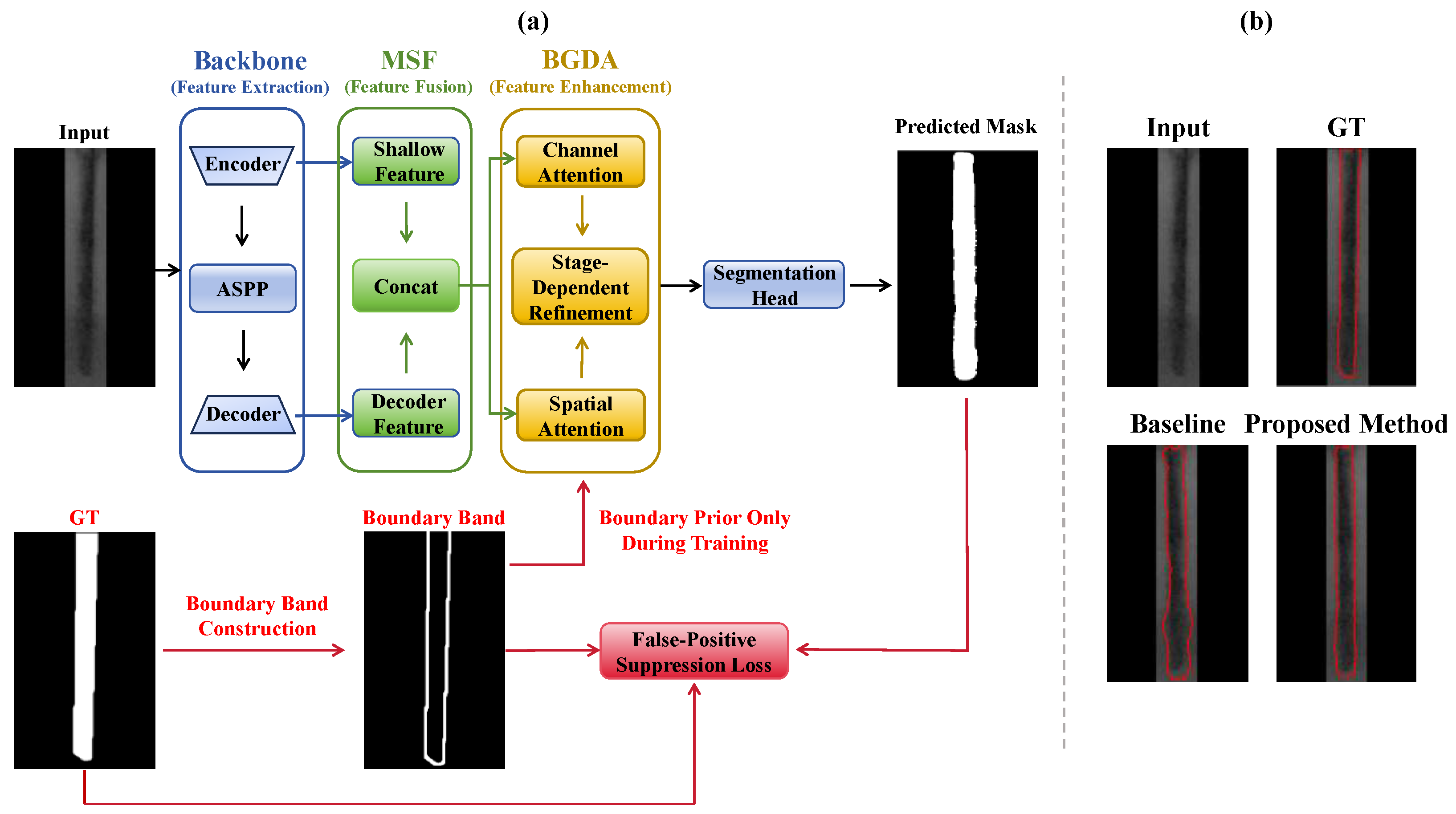
Deep learning has achieved substantial progress in semantic segmentation and has been widely used for dense pixel-level prediction in various image analysis tasks. Among these methods, encoder–decoder architectures, such as U-Net [10] and DeepLab [11], have become representative segmentation frameworks because they combine end-to-end representation learning with multi-scale contextual modeling [12,13]. However, directly applying these general segmentation models to weld radiographic defect segmentation remains challenging. Weld defects may be thin, elongated, or irregular, and their boundaries are often blurred by low contrast, uneven illumination, imaging noise, and complex weld seam backgrounds. In addition, weld seams, noise patterns, and imaging artifacts may exhibit defect-like grayscale responses, which easily induce false-positive foreground activations. As shown in Figure 1, one typical failure mode of existing segmentation models is boundary over-expansion, where the predicted mask extends beyond the true defect contour and activates nearby background regions. Such errors are particularly problematic for weld radiographic inspection because they may overestimate the defect size and increase unnecessary manual rechecking. Existing boundary-aware methods can improve contour alignment [1,13], but many rely on auxiliary boundary branches or additional boundary supervision, which increase model complexity and may become unstable when defect boundaries are weak or ambiguous. Therefore, for weld radiographic defect segmentation, boundary emphasis needs to be selective and should be coupled with explicit suppression of false-positive responses in stable background regions.

Although boundary-aware segmentation, attention-based segmentation, and false-positive suppression strategies have been widely explored in general semantic segmentation, they do not directly solve the coupled challenges in weld radiographs. Boundary-aware methods usually introduce auxiliary edge branches, boundary prediction heads, or additional boundary supervision, which may increase model complexity and become unreliable when defect contours are weak or ambiguous. Attention-based methods enhance discriminative features, but generic channel or spatial attention may also amplify weld seams, noise patterns, and defect-like background structures. False-positive suppression strategies can reduce background activations, but if applied globally they may also suppress weak defect responses and degrade recall. In contrast, the proposed method uses annotation-derived boundary bands only as training-time regularization signals to guide attention-driven feature modulation, while the deployed model requires only the input radiograph. Moreover, false-positive suppression is applied specifically to stable non-boundary background regions, thereby reducing over-expanded predictions without over-penalizing ambiguous boundary pixels. The distinction from representative boundary-aware and false-positive suppression strategies is further examined through mechanism-level comparison and controlled loss-level experiments in Section 4.6.

To address these issues, we propose a boundary-guided feature modulation framework with false-positive suppression for weld radiographic defect segmentation. The method combines multi-scale feature fusion (MSF), a boundary-guided dual attention (BGDA) module, and a false-positive suppression loss (FPL). Specifically, MSF aggregates semantic and decoder features to recover weak defect responses. BGDA employs stage-dependent refinement (SDR) to regularize attention-driven feature enhancement during training and performs boundary-free refinement during inference. FPL constrains erroneous foreground activations in non-boundary background regions. Experiments are conducted on a large-scale real-world industrial weld radiographic dataset containing 10,079 annotated images. The results show that the proposed method improves Dice and Precision over representative baselines while maintaining competitive Recall. Qualitative results further demonstrate more coherent defect boundaries and cleaner background predictions. The main contributions of this work are summarized as follows:

• The relatively underexplored task of pixel-level weld radiographic defect segmentation is investigated, with emphasis on its importance for precise defect-region delineation and weld-quality assessment.
• A boundary-guided feature modulation framework is developed, in which multi-scale feature fusion and BGDA with SDR are integrated to achieve boundary-guided residual refinement during training and boundary-free refinement during inference.
• A false-positive suppression loss is designed so that erroneous foreground responses in stable non-boundary background regions are penalized, improving the Dice–Precision trade-off in weld radiographic defect segmentation.

2. Related Work

This section reviews related work in three directions: weld defect detection, weld defect classification, and X-ray defect segmentation. Detection and classification methods provide useful localization or qualitative recognition results, but they usually cannot describe the precise spatial extent and boundary shape of weld defects. Therefore, we further discuss segmentation-oriented studies and their limitations in handling weak boundaries, foreground–background imbalance, and defect-like background responses, which motivates the proposed boundary-guided segmentation framework.

2.1. Weld Defect Detection

Weld defect detection is essential in automated non-destructive testing for providing location information required by subsequent quality assessment. Early radiographic analysis relied on handcrafted operations such as thresholding, edge detection, morphology, and texture descriptors [14]. Although intuitive and efficient, these methods are sensitive to image contrast, noise, and manual parameter tuning, limiting their robustness on real industrial radiographs with complex backgrounds and diverse defect appearances.

Recently, convolutional neural networks have been increasingly adopted for weld defect detection [4,5,6], learning task-specific features directly from images and better handling variations in defect morphology and background. However, detection-based methods typically output bounding boxes, heat maps, or coarse regions, which lack exact defect contours. Such coarse localization is often insufficient for downstream quantitative assessment, particularly for thin, elongated, low-contrast, or structurally adjacent defects. Consequently, detection-level outputs cannot fully replace pixel-level segmentation for fine-grained weld radiographic analysis.

2.2. Weld Defect Classification

Another major direction is weld defect classification, which qualitatively identifies defect presence and types (e.g., cracks, porosity, slag inclusion, lack of fusion, incomplete penetration, undercut, concavity). These studies aid diagnosis and reporting [6,7], sometimes employing heat maps or attention mechanisms to improve interpretability [6].

While valuable for linking defect types to formation mechanisms and inspection decisions, classification typically operates at the image, patch, or region level. It indicates defect presence or type but cannot accurately delineate spatial extent, boundaries, or area. Since precise geometric information is crucial for subsequent measurement and severity assessment, classification complements but cannot replace pixel-level segmentation.

2.3. Weld Defect Segmentation

Semantic segmentation aims to assign a pixel-level label to each image location and is therefore more suitable for estimating defect area, contour, and spatial distribution. Encoder–decoder architectures, such as U-Net [10] and DeepLab [11], have become representative baselines for dense prediction because they combine semantic abstraction with spatial detail recovery. U-Net variants and interactive segmentation frameworks have also been explored for defect segmentation tasks [8,9]. In X-ray or radiographic inspection scenarios, segmentation is particularly meaningful because defects often appear as subtle grayscale discontinuities, and their exact boundaries are needed for quantitative analysis.

However, compared with weld defect detection and qualitative recognition, dedicated studies on pixel-level weld radiographic defect segmentation remain relatively limited. Existing segmentation models still face several difficulties when applied to weld radiographs. First, defect pixels usually occupy a small proportion of the image, causing severe foreground–background imbalance. Second, defect boundaries are often weak, blurred, or uncertain because of low contrast, uneven illumination, noise, and imaging artifacts. Third, weld seams and background textures may exhibit defect-like grayscale responses, leading to false-positive predictions and boundary over-expansion. Generic multi-scale fusion or attention mechanisms can recover weak defect responses, but they may also amplify confusing background structures if they are not constrained by defect boundary characteristics.

Therefore, weld radiographic defect segmentation requires methods that not only recover weak defect regions but also handle ambiguous boundaries and suppress false positives in stable background areas. Motivated by this gap, this study focuses on the relatively underexplored problem of pixel-level weld radiographic defect segmentation and proposes a boundary-guided feature modulation framework with false-positive suppression. Unlike classification or detection methods that provide only image-level labels, heat maps, or bounding boxes, the proposed framework is designed to generate accurate defect masks with cleaner background predictions, supporting more reliable downstream weld radiographic assessment.

3. Methodology

This section presents the proposed boundary-guided feature modulation framework with false-positive suppression. The method consists of boundary band construction, multi-scale feature fusion (MSF), boundary-guided dual attention (BGDA) with stage-dependent refinement (SDR), and a region-aware optimization strategy.

3.1. Boundary Band Construction and Modeling

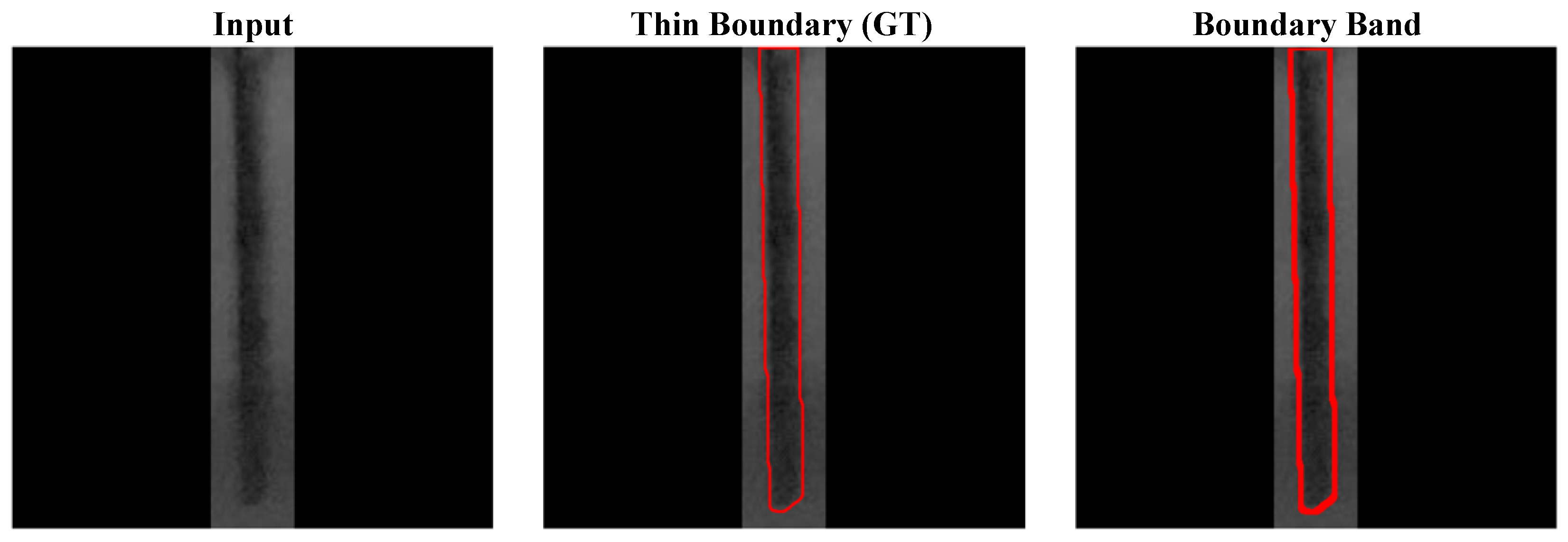
Instead of using idealized one-pixel contours, we model defect boundaries as a narrow uncertainty band to tolerate annotation noise and blurred foreground–background transitions. Given a ground-truth mask Y, let $Y_{\mathrm{bd}}$ denote its thin boundary map. The binary boundary band is defined as $B=\mathrm{Dilate}(Y_{\mathrm{bd}},r)$, where r controls the band width and $B_{i,j}=1$ indicates that pixel $(i,j)$ lies in the boundary band. As illustrated in Figure 2, the thin ground-truth boundary is dilated to generate a narrow band covering the uncertain foreground–background transition around the defect contour. During training, B serves as a boundary prior for SDR and region-aware loss construction. During inference, this training-time boundary prior is not used, and the model requires only the input radiograph without any ground-truth.

3.2. Boundary-Guided Dual Attention

Building upon the constructed boundary band, we introduce BGDA to regulate attention-driven feature amplification. Generic channel or spatial attention reweights the whole feature map and may amplify homogeneous background responses in weld radiographs. Since segmentation errors are mainly concentrated near foreground–background transitions, BGDA uses the training-time boundary prior to regularize attention-driven feature enhancement toward boundary-adjacent regions.

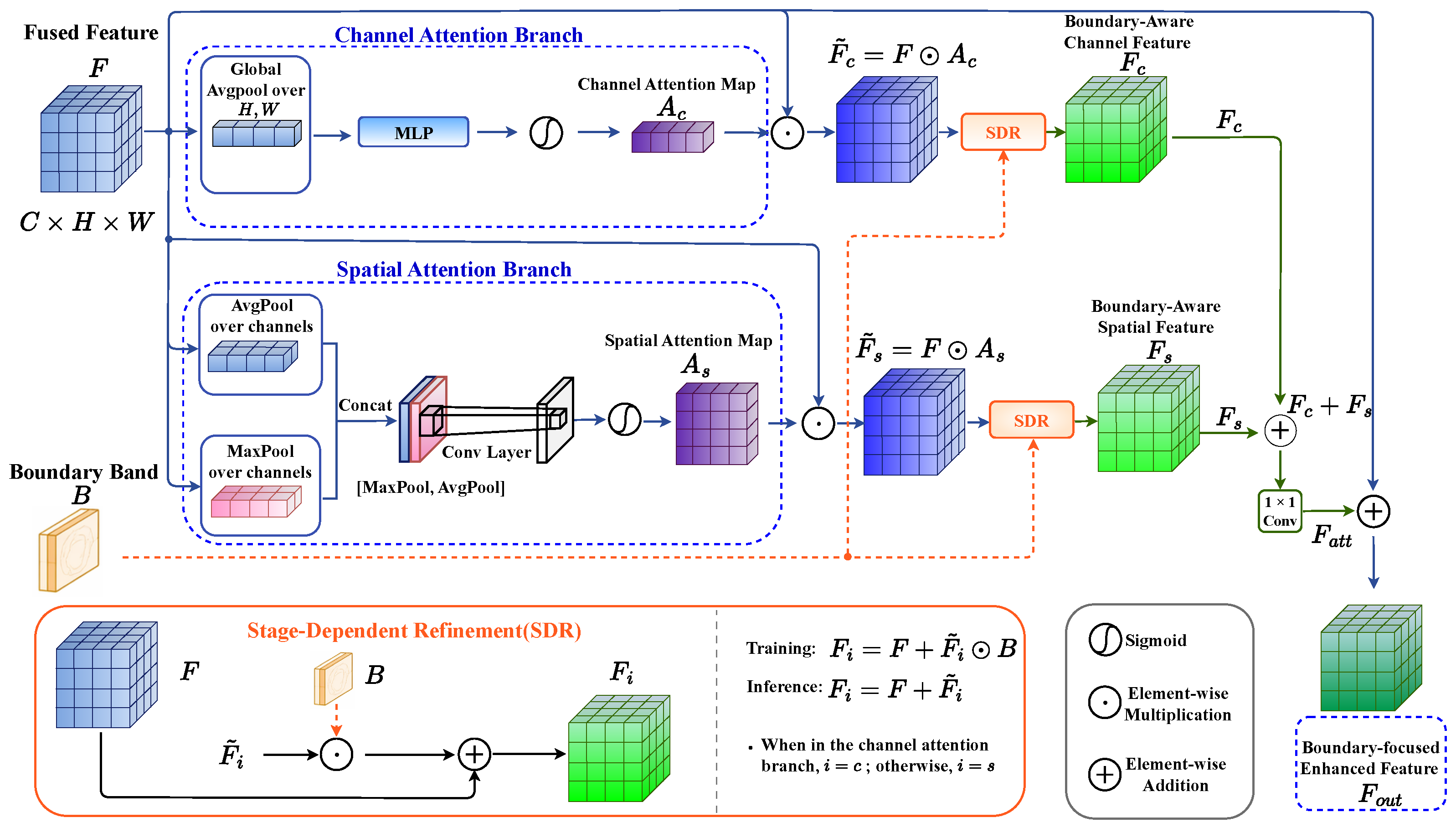
As illustrated in Figure 3, BGDA consists of channel and spatial descriptor-learning branches followed by a stage-dependent refinement operator. Given a fused feature map $F\in {\mathbb{R}}^{C\times H\times W}$, the channel attention branch first computes $A_c=\sigma \left(\mathrm{MLP}\left(\mathrm{GAP}\left(F\right)\right)\right)$, where $A_c\in {\mathbb{R}}^{C\times 1\times 1}$ denotes the learned channel-wise attention weights. The MLP adopts a bottleneck structure with reduction ratio $\rho$.

In parallel, the spatial attention branch computes a spatial descriptor $A_s=\sigma \left({\mathrm{Conv}}_{7\times 7}\left([{\mathrm{AvgPool}}_c\left(F\right);{\mathrm{MaxPool}}_c\left(F\right)]\right)\right)$, where $A_s\in {\mathbb{R}}^{1\times H\times W}$ denotes the spatial attention response.

The two descriptors first modulate the fused feature map as ${\tilde{F}}_c=F\odot A_c,{\tilde{F}}_s=F\odot A_s$, where the attention maps are broadcast to match the size of F. We define the subsequent residual refinement as stage-dependent refinement (SDR), which adopts different forms during training and inference:

$$\mathrm{SDR}(F,{\tilde{F}}_i,B)=\left\{\begin{array}{cc}F+{\tilde{F}}_i\odot B,\hfill & \mathrm{during}\mathrm{training},\hfill \\ F+{\tilde{F}}_i,\hfill & \mathrm{during}\mathrm{inference},\hfill \end{array}\right.i\in \{c,s\}.$$

(1)

Here, B is the boundary band constructed from the ground-truth mask and is available only during training. Therefore, SDR performs boundary-guided residual refinement during training and boundary-free residual refinement during inference.

3.2.1. Training Mode of SDR: Boundary-Guided Refinement

During training, the boundary band is available from the ground-truth mask and is used as a binary gate to restrict attention-driven feature amplification to boundary-adjacent regions. For $i\in \{c,s\}$, the training-time refinement operator is defined as

$${\mathcal{R}}_{\mathrm{train}}(F,A_i,B)=F+(F\odot A_i)\odot B,i\in \{c,s\},$$

(2)

where $B\in {\{0,1\}}^{1\times H\times W}$ denotes the boundary band resized to the spatial resolution of F and broadcast along the channel dimension. The refined channel and spatial features are then obtained by $F_c={\mathcal{R}}_{\mathrm{train}}(F,A_c,B),F_s={\mathcal{R}}_{\mathrm{train}}(F,A_s,B)$. This design makes the boundary band act as a training-time regularizer for attention learning, encouraging the module to emphasize boundary-sensitive responses while avoiding unrestricted amplification of background textures.

3.2.2. Inference Mode of SDR: Boundary-Free Refinement

At inference time, the boundary band is unavailable and is not estimated by an auxiliary branch. To avoid any dependence on ground-truth-derived boundary information, the boundary gate is removed, while the learned channel and spatial attention descriptors are kept unchanged. The inference-time refinement operator is therefore defined as

$${\mathcal{R}}_{\inf }(F,A_i)=F+F\odot A_i,i\in \{c,s\}.$$

(3)

Accordingly, the channel and spatial refined features during inference are computed as $F_c={\mathcal{R}}_{\inf }(F,A_c),F_s={\mathcal{R}}_{\inf }(F,A_s)$. Thus, BGDA uses boundary information only during training, whereas the deployed model requires only the input radiograph and does not use any ground-truth or predicted boundary mask.

The refined features are then fused by a $1\times 1$ convolution: $F_{\mathrm{att}}={\mathrm{Conv}}_{1\times 1}(F_c+F_s)$. Finally, a residual connection is applied to preserve the original semantics: $F_{\mathrm{out}}=F+F_{\mathrm{att}}$.

In this way, descriptor learning and boundary-guided regularization are decoupled: the former provides complementary channel and spatial attention cues for both training and inference, while the latter is used only during training to guide feature enhancement around ambiguous defect boundaries.

3.3. Boundary-Guided Optimization Strategy

BGDA improves feature representation near ambiguous contours, but feature modulation alone does not fully control the precision–recall trade-off. In practice, pixels near foreground–background transitions are intrinsically ambiguous, whereas non-boundary background regions are comparatively stable. This motivates a region-aware optimization strategy consisting of boundary-weighted supervision and explicit false-positive suppression.

3.3.1. Boundary-Weighted Segmentation Loss

Let $P_{i,j}\in [0,1]$ denote the predicted foreground probability at location $(i,j)$, and let $Y_{i,j}\in \{0,1\}$ be the corresponding ground-truth label. A boundary-weighting map is defined as

$$W_{i,j}=\left\{\begin{array}{cc}\alpha ,\hfill & B_{i,j}=1,\hfill \\ 1,\hfill & \mathrm{otherwise},\hfill \end{array}\right.$$

(4)

where $\alpha >1$ controls the relative importance assigned to boundary-adjacent pixels.

Using this weighting map, the boundary-weighted binary cross-entropy loss (BW-BCE) is formulated as

$${\mathcal{L}}_{\mathrm{BCE}}^{\mathrm{bw}}=-{\displaystyle \frac{1}{N}}{\displaystyle \sum _{i,j}}{W}_{i,j}\left[Y_{i,j}\log P_{i,j}+(1-Y_{i,j})\log (1-P_{i,j})\right],$$

(5)

where $N=H\times W$ denotes the number of spatial locations.

To further encourage contour consistency and alleviate class imbalance, we also employ a boundary-weighted Dice loss (BW-Dice):

$${\mathcal{L}}_{\mathrm{Dice}}^{\mathrm{bw}}=1-{\displaystyle \frac{2{\sum }_{i,j}{W}_{i,j}{P}_{i,j}{Y}_{i,j}}{{\sum }_{i,j}{W}_{i,j}{P}_{i,j}+{\sum }_{i,j}{W}_{i,j}{Y}_{i,j}+ϵ}},$$

(6)

where $ϵ$ is a small constant for numerical stability. The combined boundary-weighted segmentation loss is defined as ${\mathcal{L}}_{\mathrm{BW}}={\mathcal{L}}_{\mathrm{BCE}}^{\mathrm{bw}}+{\mathcal{L}}_{\mathrm{Dice}}^{\mathrm{bw}}.$

By strengthening supervision at boundary-adjacent locations, this loss improves boundary alignment and complements the subsequent false-positive suppression term, helping achieve a better precision–recall trade-off.

3.3.2. False-Positive Suppression in Non-Boundary Background Regions

Boundary-weighted losses emphasize ambiguous transitions but do not explicitly penalize overconfident foreground responses in stable background regions. We therefore define the non-boundary background set as ${\mathcal{R}}_{\mathrm{bg}}=\{(i,j)\mid Y_{i,j}=0,B_{i,j}=0\}$ and introduce

$${\mathcal{L}}_{\mathrm{FP}}={\displaystyle \frac{1}{|{\mathcal{R}}_{\mathrm{bg}}|+ϵ}}{\displaystyle \sum _{(i,j)\in {\mathcal{R}}_{\mathrm{bg}}}}\max (0,P_{i,j}-\tau ),$$

(7)

where $\tau \in (0,1)$ is the tolerated foreground-confidence margin. This loss penalizes only non-boundary background pixels whose predicted foreground probability exceeds $\tau$.

Combining the boundary-weighted segmentation loss and the false-positive suppression loss, the overall training objective is given by

$$\mathcal{L}={\lambda }_{\mathrm{bw}}{\mathcal{L}}_{\mathrm{BW}}+{\lambda }_{\mathrm{fp}}{\mathcal{L}}_{\mathrm{FP}},$$

(8)

where ${\lambda }_{\mathrm{bw}}$ and ${\lambda }_{\mathrm{fp}}$ control the relative contributions of boundary-weighted segmentation supervision and false-positive suppression, respectively.

3.4. Overall Framework

Overall, the proposed framework follows an encoder–decoder segmentation pipeline with boundary-guided feature modulation. Given an input radiograph, hierarchical features are first extracted and decoded by the base DeepLabV3+ network to generate a semantic decoder representation for dense defect prediction.

To enhance weak defect responses, MSF is used to fuse the decoder representation with shallow spatial-detail cues. The involved features are projected to a common feature space, spatially aligned, concatenated, and transformed by convolutional operations, yielding the fused feature representation.

The fused feature is subsequently fed into BGDA for boundary-aware feature refinement. The channel attention branch and spatial attention branch learn complementary attention descriptors from the fused feature. During training, the boundary band generated from the ground-truth mask is resized to the BGDA feature resolution and used as a training-time prior in SDR, so that attention-driven residual refinement is guided toward boundary-adjacent regions. The same boundary band is also used for region-aware loss construction, including boundary-weighted supervision and false-positive suppression in stable non-boundary background regions.

After BGDA, the boundary-focused enhanced feature is passed to the segmentation head, which consists of a $3\times 3$ convolution with batch normalization and ReLU, an upsampling operation, and a final $1\times 1$ convolution to generate the defect mask prediction. During inference, no boundary band is generated or predicted. The model removes the boundary gate in SDR and performs boundary-free residual refinement using only the learned channel and spatial attention descriptors, so the deployed model requires only the input radiograph.

4. Results and Discussion

4.1. Experimental Setup

This subsection describes the experimental protocol used to evaluate the proposed method. We first introduce the weld radiographic dataset, including its defect categories, data split, and image preprocessing. We then present the implementation details, including the backbone configuration, training strategy, data augmentation, and hyperparameter settings. Finally, we define the evaluation metrics used to assess both region-level segmentation accuracy and boundary alignment. Unless otherwise specified, the same data split, input resolution, and evaluation protocol are used throughout the experiments to ensure fair and reproducible comparisons.

4.1.1. Dataset

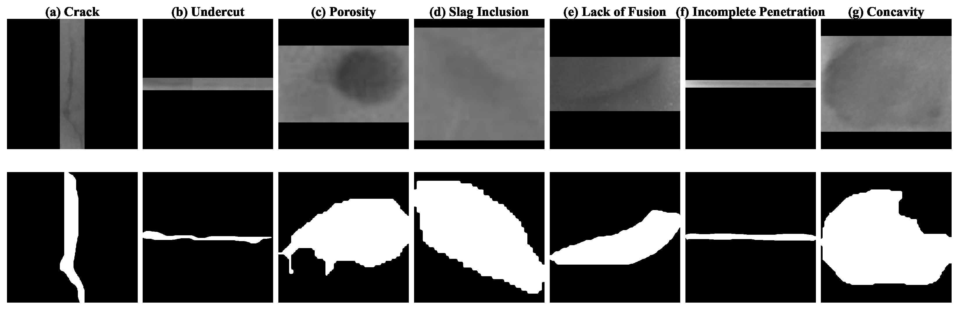
Experiments are conducted on a proprietary weld radiographic dataset containing 10,079 annotated defect-containing regions of interest (ROIs) collected from real-world pipeline weld inspection environments. In this study, an ROI refers to a radiographic image region containing a visible weld defect and its surrounding weld background, and each ROI is treated as one image sample for training, validation, and testing. The dataset covers seven common weld defect categories, including Crack, Undercut, Porosity, Slag inclusion, Lack of fusion, Incomplete penetration, and Concavity. As summarized in

Table 1. Distribution of defect categories in the weld radiographic dataset. The dataset contains 10,079 annotated images covering seven common weld defect types, with category proportions ranging from 12.0% to 16.4%, indicating an approximately balanced class composition.

Defect Class	Count	Ratio
Crack	1653	16.4%
Undercut	1552	15.4%
Porosity	1472	14.6%
Slag inclusion	1461	14.5%
Lack of fusion	1441	14.3%
Incomplete penetration	1290	12.8%
Concavity	1210	12.0%
Total	10,079	100.0%

, the category proportions range from 12.0% to 16.4%, indicating an approximately balanced class composition. Representative radiographic examples and their corresponding pixel-level annotation masks are shown in Figure 4.

The pixel-level defect annotations were produced by two annotation experts with experience in weld radiographic inspection. For each defect-containing ROI, the visible defect region was manually delineated as a binary mask, where foreground pixels correspond to the defective region and background pixels correspond to non-defective weld or surrounding structures. The annotation process focused on the physically interpretable defect extent rather than on an idealized one-pixel contour, because weld radiographic defects often exhibit weak contrast, gradual grayscale transitions, and blurred boundaries.

To ensure annotation quality, the masks were further checked through a review procedure. During quality control, the reviewers examined defect presence, category consistency, mask completeness, and boundary plausibility by comparing the binary masks with the original radiographic ROIs. Cases with incomplete masks, obvious boundary over-extension, missed weak defect regions, or inconsistent defect categories were returned for correction. The final accepted masks after review were used as the ground-truth annotations in this study. Since the proposed method constructs boundary bands from the training annotations, special attention was paid to boundary reliability during annotation verification. Nevertheless, the radiographic transition between defect and background is sometimes intrinsically ambiguous. Therefore, the ground-truth boundary should be interpreted as an expert-verified defect extent rather than as an absolutely sharp physical edge.

The radiographs were acquired under practical industrial non-destructive testing (NDT) conditions rather than under a fixed laboratory imaging setup. As a result, the dataset contains acquisition variability caused by different inspection cases, exposure conditions, imaging geometries, weld seam appearances, and fields of view. These factors lead to variations in grayscale contrast, local background texture, noise level, defect morphology, and boundary ambiguity. Such variability reflects the practical difficulty of weld radiographic defect segmentation and is one reason why boundary-aware regularization is necessary.

The inspected products are pipeline welds collected from industrial radiographic inspection scenarios. The anonymized product records cover medium- and large-diameter pipeline welds, with pipe outer diameters of approximately 114–610 mm, wall thicknesses of approximately 6–25 mm, and visible weld seam widths of approximately 8–30 mm in the radiographic regions of interest. Exact product identifiers and detailed acquisition records are not disclosed because of confidentiality restrictions imposed by the industrial data provider.

To provide an approximate physical interpretation of the defect scale, we estimated the image-plane size of the original defect-containing ROIs on the scanned radiographs. The original defect-containing ROIs have side lengths of approximately 50–200 pixels. Given an approximate film scanning resolution of 300 dpi, one pixel corresponds to about $25.4/300\approx 0.085$ mm on the scanned film plane; therefore, these ROIs cover a physical scale of approximately $4.2$–$16.9$ mm along one spatial dimension. Since the ROI size is not identical to the true defect size and may include surrounding margins, the actual physical size depends on the defect morphology and the ROI margin.

For elongated defects, the estimated major-axis length and minor-axis width are approximately $4.2$–$16.9$ mm and $0.6$–$2.4$ mm, respectively, when the long axis is comparable to the ROI side length. For compact defects with nearly equal length and width, the characteristic diameter or side length is approximately $4.2$–$16.9$ mm. These estimates provide an approximate physical interpretation of the defect scale on the scanned radiographs, rather than a fully calibrated object-space measurement, because the exact acquisition geometry and magnification parameters are not available for all inspection cases.

Before being fed into the segmentation models, all radiographic ROIs and their corresponding masks are resized to $512\times 512$ pixels. Bilinear interpolation is used for radiographic images, whereas nearest-neighbor interpolation is used for binary masks to preserve pixel-level labels. All model training and evaluation are performed in the resized pixel space.

4.1.2. Implementation Details

The proposed method is implemented in PyTorch 2.6.0 and trained on an NVIDIA RTX 3090 GPU. DeepLabV3+ with an ImageNet-pretrained ResNet-101 encoder is used as the representative backbone. The 10,079 annotated defect-containing ROI images were stratified by defect category and split at the ROI level into training, validation, and test subsets with an 8:1:1 ratio, respectively. This stratified split approximately preserves the overall defect-category distribution in each subset. To ensure comparison fairness and reproducibility, all methods use this same split, an input resolution of $512\times 512$, the same data augmentation strategy, a batch size of 16 and a training schedule of 100 epochs, validation-Dice-based checkpoint selection, an inference threshold of 0.5, and the same evaluation protocol.

A family-level grouped optimization protocol is adopted for the architecture comparison. Specifically, CNN/ResNet-based methods, including U-Net, UNet++, Attention U-Net, UNet3+, DeepLabV3+, and the proposed model, are trained using SGD with momentum 0.9, an initial learning rate of $1\times {10}^{-3}$, weight decay of $1\times {10}^{-4}$, and a poly learning-rate schedule with power 0.9. Transformer-based methods, including Swin-UNet, SegFormer, and DPT, are trained using AdamW with an initial learning rate of $6\times {10}^{-5}$, weight decay of $1\times {10}^{-2}$, and linear warm-up followed by poly decay. The non-proposed baselines are trained with the BCE–Dice loss, whereas the proposed method uses the proposed boundary-weighted BCE–Dice loss and false-positive suppression loss with $r=3$, $\alpha =2.0$, $\tau =0.1$, ${\lambda }_{\mathrm{bw}}=0.3$, and ${\lambda }_{\mathrm{fp}}=1.0$. No hyperparameter is tuned on the test set.

To evaluate the repeatability and stability of the reported results, each segmentation model is independently trained three times with different random seeds. Across the three runs, we use the same training, validation, and test splits. Only the random seed is changed, which affects weight initialization, the order of training samples, and random data augmentation. Unless otherwise specified, the quantitative results in the comparison, per-category, ablation, and loss comparison tables are reported as mean ± standard deviation over the three independent runs. Best and second-best results are determined according to the mean value.

4.1.3. Evaluation Metrics

Segmentation performance is assessed using three commonly adopted pixel-level metrics, namely Dice coefficient, Precision, and Recall. The predicted probability map is binarized with a threshold of $0.5$ before metric calculation. Dice, Precision, and Recall are computed for each image and then averaged over the corresponding evaluation split. Therefore, the reported Dice is not necessarily equal to the harmonic mean of the averaged Precision and Recall.

In addition to region-level metrics, we report the Surface Dice at tolerance $\delta$ (SD_δ) to evaluate boundary alignment. This metric is used because weld radiographic defects often have blurred and ambiguous contours, and small boundary deviations may be caused by annotation uncertainty or low-contrast foreground–background transitions. Unlike region-overlap metrics such as Dice, SD_δ directly evaluates whether the predicted contour is located within an acceptable distance from the ground-truth contour, making it more suitable for assessing boundary over-expansion and contour localization.

The boundaries of the ground-truth and predicted masks are extracted by subtracting the eroded mask from the original binary mask. Let $\partial Y$ and $\partial \widehat{Y}$ denote the boundaries of the ground-truth mask and the predicted mask, respectively. For a boundary pixel p and a boundary set $\partial S$, let $d(p,\partial S)$ denote the Euclidean distance from p to its nearest pixel in $\partial S$. The matched predicted and ground-truth boundary pixels under tolerance $\delta$ are defined as

$$M_{\widehat{Y}}^{\delta }=\{p\in \partial \widehat{Y}\mid d(p,\partial Y)\le \delta \},$$

(9)

and

$$M_Y^{\delta }=\{q\in \partial Y\mid d(q,\partial \widehat{Y})\le \delta \}.$$

(10)

The Surface Dice at tolerance $\delta$ is then computed as

$$S{D}_{\delta }={\displaystyle \frac{|M_{\widehat{Y}}^{\delta }|+|M_Y^{\delta }|}{|\partial \widehat{Y}|+|\partial Y|+ϵ}}.$$

(11)

In our experiments, $\delta$ is set to 3 pixels, which is consistent with the boundary-band width used in the proposed boundary modeling strategy. We denote this metric as SD_3px in the following tables. SD_3px is computed for each image and then averaged over the evaluation split.

4.1.4. Statistical Testing Protocol

To examine whether the observed performance gains are statistically meaningful, we further conducted image-wise paired statistical significance analysis on the same test set. For each method and each evaluation metric, the metric value was first computed for each test image in each of the three independent runs. To avoid treating repeated random seeds as independent test samples, we averaged the three runs for each test image and obtained one image-wise score per method. For a given metric, paired differences were then computed between the proposed method and the corresponding comparison method on the same test images.

Because segmentation metrics such as Dice, Precision, Recall, and SD_3px are bounded and may not strictly follow a normal distribution, we used the two-sided Wilcoxon signed-rank test for paired comparisons. In addition, 95% confidence intervals (CIs) of the mean paired differences were estimated using paired bootstrap resampling with 10,000 resamples. Holm–Bonferroni correction was applied to control the family-wise error rate when multiple comparisons were conducted within the same table. A difference was considered statistically significant when the adjusted p-value was smaller than 0.05. Positive mean differences indicate that the proposed method or the full configuration outperforms the corresponding comparison method.

4.2. Comparison with Representative Segmentation Methods

We compare the proposed method with representative CNN-based and Transformer-based segmentation models. All compared methods follow the same data split, input resolution, augmentation, training budget, checkpoint selection rule, inference threshold, and evaluation protocol, while the optimizer configuration is grouped by model family as described in the implementation details.

As shown in

Table 2. Quantitative comparison under the family-level grouped training protocol. Results are reported as mean ± standard deviation over three independent runs. The upward arrow (↑) indicates that higher values are better. Best results are shown in bold, and second-best results are underlined. ^† indicates that the proposed method is significantly better than the strongest non-proposed comparison method for the corresponding metric according to the two-sided Wilcoxon signed-rank test with Holm–Bonferroni correction ($p<0.05$).

Family	Method	Dice ↑	Precision ↑	Recall ↑	SD3px ↑
CNN-based baselines	U-Net [10]	0.746 ± 0.004	0.701 ± 0.006	0.789 ± 0.005	0.211 ± 0.014
	UNet++ [15]	0.762 ± 0.003	0.718 ± 0.005	0.804 ± 0.004	0.235 ± 0.009
	Attention U-Net [16]	0.772 ± 0.004	0.728 ± 0.006	0.816 ± 0.005	0.251 ± 0.007
	UNet3+ [17]	0.783 ± 0.003	0.742 ± 0.005	0.826 ± 0.004	0.270 ± 0.016
	DeepLabV3+	0.788 ± 0.003	0.756 ± 0.004	0.823 ± 0.004	0.289 ± 0.006
Transformer-based baselines	Swin-UNet [18]	0.786 ± 0.004	0.751 ± 0.006	0.825 ± 0.005	0.284 ± 0.007
	SegFormer [19]	0.784 ± 0.004	0.742 ± 0.005	0.829 ± 0.004	0.278 ± 0.008
	DPT [20]	0.789 ± 0.005	0.739 ± 0.006	0.836 ± 0.005	0.269 ± 0.011
Proposed	Proposed Method	0.810 ± 0.003 †	0.809 ± 0.004 †	0.812 ± 0.004	0.394 ± 0.008 †

, classical encoder–decoder models and Transformer-based baselines generally achieve competitive Recall, but their Precision and SD_3px values remain lower than those of the proposed method. This indicates that these models can locate many defect pixels, but they are more likely to activate defect-like background regions or produce over-expanded contours. For example, DPT obtains the highest Recall, but its lower Precision and SD_3px suggest that the improvement in foreground coverage is accompanied by less accurate background suppression and weaker boundary localization.

The proposed method achieves the best Dice, Precision, and SD_3px while maintaining competitive Recall. From a methodological perspective, this behavior is consistent with the design of the proposed framework. MSF aggregates semantic and spatial-detail features, which helps preserve weak defect responses that may otherwise be missed by a single-scale decoder. BGDA further regularizes attention-driven feature refinement using the training-time boundary band, encouraging the model to focus on boundary-adjacent regions rather than amplifying background textures indiscriminately. Finally, FPL penalizes overconfident foreground responses in stable non-boundary background regions. Therefore, the improvement in Dice mainly comes from a better balance between defect recovery and false-positive suppression, while the improvement in SD_3px reflects more reliable contour localization. Beyond the relatively small standard deviations across three independent runs, the image-wise paired statistical analysis further confirms that the main improvements are statistically meaningful. Specifically, the proposed method achieves significant improvements in Dice, Precision, and SD_3px over the strongest non-proposed counterparts, with all adjusted p-values smaller than 0.05 and the corresponding 95% confidence intervals excluding zero. This indicates that the reported gains are unlikely to be caused by random initialization or test sample variation alone.

4.3. Per-Category Performance Analysis

Table 3. Per-category performance of the proposed method on the test set. Results are reported as mean ± standard deviation over three independent runs. The upward arrow (↑) indicates that higher values are better. The ratio column reports the category proportion, which approximately follows the overall dataset distribution under the stratified split.

Defect Type	Ratio (%)	Dice ↑	Precision ↑	Recall ↑	SD3px ↑
Crack	16.4	0.787 ± 0.010	0.768 ± 0.011	0.807 ± 0.010	0.340 ± 0.021
Undercut	15.4	0.823 ± 0.005	0.825 ± 0.006	0.822 ± 0.006	0.409 ± 0.010
Porosity	14.6	0.826 ± 0.004	0.840 ± 0.006	0.813 ± 0.005	0.423 ± 0.009
Slag inclusion	14.5	0.811 ± 0.005	0.818 ± 0.007	0.805 ± 0.006	0.407 ± 0.010
Lack of fusion	14.3	0.809 ± 0.006	0.804 ± 0.007	0.815 ± 0.006	0.389 ± 0.011
Incomplete penetration	12.8	0.814 ± 0.005	0.807 ± 0.006	0.822 ± 0.006	0.413 ± 0.016
Concavity	12.0	0.801 ± 0.006	0.804 ± 0.007	0.799 ± 0.007	0.383 ± 0.012

presents the per-category performance of the proposed method. The proposed method maintains stable segmentation performance across different weld defect categories, but the metric variations are closely related to defect morphology and boundary ambiguity. Porosity, undercut, and incomplete penetration obtain relatively high Dice and SD_3px values, suggesting that their defect regions are more separable from the surrounding weld background and their contours can be more consistently localized. In these cases, MSF helps preserve local defect responses, while BGDA and FPL reduce boundary over-expansion and background activations.

In contrast, crack defects obtain lower Dice and SD_3px values because cracks are often thin, elongated, and weakly contrasted in radiographic images. For such defects, a small boundary deviation or slight discontinuity can cause a relatively large decrease in overlap-based and boundary-based metrics. This result indicates that the proposed method improves the overall Dice–Precision–boundary trade-off, but extremely thin and low-contrast defects remain challenging. The generally small standard deviations suggest that the proposed method remains stable across repeated runs for different defect categories.

4.4. Ablation Study

Table 4. Ablation study of different components. Results are reported as mean ± standard deviation over three independent runs. The upward arrow (↑) indicates that higher values are better. The symbols ✓ and × indicate that the corresponding component is used and not used, respectively. Best results are shown in bold. ^† indicates that the full model is significantly better than the MSF+BGDA variant for the corresponding metric according to the two-sided Wilcoxon signed-rank test with Holm–Bonferroni correction ($p<0.05$).

MSF	BGDA	FPL	Dice ↑	Precision ↑	Recall ↑	SD3px ↑
×	×	×	0.788 ± 0.003	0.756 ± 0.004	0.823 ± 0.004	0.289 ± 0.006
✓	×	×	0.787 ± 0.004	0.745 ± 0.006	0.834 ± 0.005	0.314 ± 0.017
✓	✓	×	0.798 ± 0.003	0.776 ± 0.005	0.819 ± 0.004	0.365 ± 0.011
✓	×	✓	0.795 ± 0.004	0.787 ± 0.005	0.802 ± 0.005	0.350 ± 0.008
✓	✓	✓	0.810 ± 0.003 †	0.809 ± 0.004 †	0.812 ± 0.004	0.394 ± 0.008 †

reports incremental ablations of MSF, BGDA, and FPL under the same DeepLabV3+ setting. The baseline corresponds to DeepLabV3+ without these components. Adding MSF increases Recall from 0.823 to 0.834, which indicates that multi-scale feature aggregation helps recover weak or partially missing defect responses. However, Precision decreases from 0.756 to 0.745, suggesting that simply enriching multi-scale features may also introduce additional responses from defect-like weld seams or background textures. This result is consistent with the motivation that weak-defect recovery alone is insufficient for reliable weld radiographic segmentation.

When BGDA is added on top of MSF, Dice increases from 0.787 to 0.798 and SD_3px increases from 0.314 to 0.365. This improvement suggests that boundary-guided attention regularization helps convert the additional feature responses introduced by MSF into more boundary-consistent predictions. In other words, BGDA does not merely strengthen features globally; instead, the training-time boundary band guides attention-driven residual refinement toward boundary-adjacent regions, which improves contour localization and reduces unrestricted background amplification.

FPL further improves Precision by explicitly penalizing overconfident foreground responses in stable non-boundary background regions. Compared with MSF+BGDA, adding FPL increases Precision from 0.776 to 0.809 and Dice from 0.798 to 0.810, while Recall remains competitive. This indicates that FPL does not simply suppress all uncertain pixels; rather, it targets non-boundary background regions where false positives are less likely to correspond to true ambiguous defect boundaries. The combination of MSF, BGDA, and FPL therefore provides complementary effects: MSF improves weak-defect recovery, BGDA improves boundary-sensitive feature refinement, and FPL improves background cleanliness. This explains why the full model achieves the best Dice, Precision, and SD_3px.

4.5. Hyperparameter Sensitivity Analysis

To address the influence of the main hyperparameters, we conducted a compact sensitivity analysis on the validation set. Instead of performing an exhaustive grid search, which would be computationally expensive and unnecessary for the purpose of robustness assessment, we grouped the hyperparameters according to their functional roles. Specifically, r, $\alpha$, and ${\lambda }_{\mathrm{bw}}$ jointly control the strength of boundary-guided supervision, whereas $\tau$ and ${\lambda }_{\mathrm{fp}}$ jointly control the strength of false-positive suppression. Therefore, we evaluated weaker and stronger settings for each functional group while keeping the other group fixed to the default setting.

As shown in

Table 5. Compact hyperparameter sensitivity analysis on the validation set. The upward arrow (↑) indicates that higher values are better. The default setting is $r=3$, $\alpha =2.0$, $\tau =0.10$, ${\lambda }_{\mathrm{bw}}=0.3$, and ${\lambda }_{\mathrm{fp}}=1.0$. Results are reported as mean ± standard deviation over three independent runs. The validation set was used for this analysis to avoid test-set-guided hyperparameter selection.

Setting	r	$\mathit{\alpha }$	$\mathit{\tau }$	${\mathit{\lambda }}_{\mathbf{bw}}$	${\mathit{\lambda }}_{\mathbf{fp}}$	Dice ↑	Precision ↑	Recall ↑	SD3px ↑
Default	3	2.0	0.10	0.3	1.0	$0.812\pm 0.006$	$0.810\pm 0.004$	$0.815\pm 0.007$	$0.397\pm 0.010$
Weaker boundary guidance	2	1.5	0.10	0.2	1.0	$0.806\pm 0.006$	$0.788\pm 0.007$	$0.823\pm 0.006$	$0.368\pm 0.005$
Stronger boundary guidance	4	2.5	0.10	0.5	1.0	$0.804\pm 0.007$	$0.815\pm 0.008$	$0.794\pm 0.009$	$0.382\pm 0.008$
Weaker FP suppression	3	2.0	0.20	0.3	0.5	$0.807\pm 0.008$	$0.783\pm 0.003$	$0.831\pm 0.007$	$0.386\pm 0.009$
Stronger FP suppression	3	2.0	0.05	0.3	1.5	$0.806\pm 0.002$	$0.827\pm 0.005$	$0.786\pm 0.012$	$0.388\pm 0.006$

, the proposed method maintains stable performance under both weaker and stronger boundary guidance and false-positive suppression. Weakening the boundary-guidance-related parameters decreases SD_3px, suggesting that insufficient boundary emphasis reduces contour alignment. Strengthening the boundary guidance slightly improves Precision but reduces Recall, indicating that excessive boundary emphasis may over-regularize ambiguous defect regions. Similarly, weaker false-positive suppression improves Recall but decreases Precision, whereas stronger false-positive suppression improves Precision at the cost of Recall.

Overall, the default setting provides the most balanced performance across Dice, Precision, Recall, and SD_3px. These results indicate that the proposed framework is not highly sensitive to a narrow hyperparameter setting and remains robust within a practical range of boundary-guidance and false-positive suppression strengths.

4.6. Comparison with Boundary-Aware and False-Positive Suppression Strategies

Although the distinction from existing boundary-aware methods has been discussed in the Introduction, we further provide a mechanism-level and quantitative comparison in this section. The purpose is not to reproduce all existing boundary-aware architectures, but to clarify how the proposed design differs from representative boundary-aware and false-positive suppression strategies in terms of boundary usage, inference requirement, and targeted error patterns.

Table 6. Mechanism-level comparison between representative boundary-aware strategies and the proposed method.

Strategy Family	Boundary or Suppression Role	Inference-Time Boundary Dependence	Relation to the Proposed Method
Auxiliary boundary branch [21]/edge head [22]	Uses an auxiliary edge or shape branch with boundary supervision	Boundary labels are not required, but an extra branch may remain in the model	The proposed method uses boundary bands only for training regularization, not as an auxiliary prediction task.
Boundary prediction head [23]	Explicitly predicts a boundary map to assist mask segmentation	A boundary representation may be generated internally during inference	The proposed method does not predict or use a boundary map at inference.
Generic attention mechanism [24]	Reweights channel or spatial features without explicit boundary supervision	No boundary-related input or prediction is required	Generic attention may also enhance seams, noise, or artifacts; BGDA is constrained by training-time boundary priors.
Boundary-oriented loss [25]	Optimizes contour distance or boundary alignment during training	No boundary-related input is required during inference	Boundary losses mainly refine contours, whereas FPL uses boundary bands to define where background suppression is safe.
Global false-positive suppression [26]	Applies image-wide or class-wide penalties to reduce background confusion	No boundary-related input is required during inference	Global suppression may weaken subtle defects; FPL restricts suppression to stable non-boundary background regions.
Proposed method	Uses boundary-band regularization for BGDA and region-aware FPL	Requires only the input radiograph during inference	Boundary guidance is training-time only, and false-positive suppression is spatially selective.

summarizes the mechanism-level differences. Existing boundary-aware segmentation methods often introduce auxiliary boundary branches, boundary prediction heads, or boundary-oriented objectives to improve contour localization. Generic attention mechanisms can enhance discriminative responses, but they do not explicitly distinguish weak defects from defect-like weld background structures. Global false-positive suppression strategies may reduce background activations, but they can also suppress weak defect responses if applied without spatial constraints. In contrast, the proposed framework uses annotation-derived boundary bands only as training-time regularization signals for attention-driven feature modulation and region-aware optimization. During inference, the deployed model requires only the input radiograph.

To quantitatively verify whether the proposed FPL provides benefits beyond conventional region-level, imbalance-aware, and boundary-aware objectives, we further compare representative loss-level strategies under the same MSF+BGDA architecture. For a fair comparison, only the loss objective is changed, while the backbone, feature modulation module, data split, training schedule, and evaluation protocol remain identical. In

Table 7. Comparison with alternative loss objectives under the same MSF+BGDA architecture. Results are reported as mean ± standard deviation over three independent runs. The upward arrow (↑) indicates that higher values are better. Best results are shown in bold. ^† indicates that BW-BCE + BW-Dice + FPL is significantly better than BW-BCE + BW-Dice for the corresponding metric according to the two-sided Wilcoxon signed-rank test with Holm–Bonferroni correction ($p<0.05$).

Loss Objective	Dice ↑	Precision ↑	Recall ↑	SD3px ↑
Std. BCE + Std. Dice	0.792 ± 0.004	0.764 ± 0.006	0.824 ± 0.005	0.323 ± 0.008
Focal [26] + Std. Dice	0.796 ± 0.003	0.782 ± 0.005	0.811 ± 0.004	0.338 ± 0.008
Active Boundary Loss [25] + Std. Dice	0.800 ± 0.003	0.783 ± 0.006	0.819 ± 0.005	0.374 ± 0.013
BW-BCE + BW-Dice	0.798 ± 0.003	0.776 ± 0.005	0.819 ± 0.004	0.365 ± 0.011
BW-BCE + BW-Dice + FPL	0.810 ± 0.003 †	0.809 ± 0.004 †	0.812 ± 0.004	0.394 ± 0.008 †

, “Std.” denotes standard unweighted losses, while “BW” denotes boundary-weighted losses.

As shown in Table 7, Std. BCE + Std. Dice achieves the highest mean Recall but lower Precision, indicating that conventional region-level supervision tends to include more ambiguous background pixels as foreground. This behavior is undesirable for weld radiographic inspection because background over-segmentation can overestimate defect size and increase unnecessary manual rechecking.

Focal loss improves Precision by emphasizing hard samples, and Active Boundary Loss improves SD_3px by introducing boundary-oriented supervision. However, these objectives do not explicitly distinguish between ambiguous boundary pixels and stable non-boundary background pixels. As a result, they can improve certain aspects of the segmentation result, but they do not directly address the specific false-positive pattern observed in weld radiographs, where weld seams, noise, and imaging artifacts may produce defect-like foreground responses away from the true defect contour.

By contrast, the proposed FPL is region-aware. It penalizes overconfident foreground probabilities only in non-boundary background regions, while avoiding excessive suppression of true defect pixels and ambiguous boundary-adjacent pixels. Adding FPL to BW-BCE + BW-Dice therefore yields the best mean Dice, Precision, and SD_3px while maintaining competitive Recall. This result supports the methodological assumption that false-positive suppression should be spatially selective rather than globally imposed.

4.7. Statistical Validation of Main Improvements

The statistical results in

Table 8. Statistical significance analysis of the main performance improvements. Mean differences are computed from image-wise paired metric values, where positive values indicate better performance of the proposed method or the full configuration. For the architecture comparison, the compared method is selected as the strongest non-proposed baseline for the corresponding metric. The 95% confidence intervals are estimated using paired bootstrap resampling with 10,000 resamples. Raw p-values are obtained using the two-sided Wilcoxon signed-rank test and then adjusted using the Holm–Bonferroni correction within each comparison group.

Comparison	Metric	Mean Difference	95% CI	Adjusted p-Value
Proposed Method vs. DPT	Dice	+0.021	[+0.015, +0.027]	0.006
Proposed Method vs. DeepLabV3+	Precision	+0.053	[+0.045, +0.061]	<0.001
Proposed Method vs. DeepLabV3+	SD3px	+0.105	[+0.089, +0.121]	<0.001
Full model vs. MSF+BGDA	Dice	+0.012	[+0.008, +0.016]	0.011
Full model vs. MSF+BGDA	Precision	+0.033	[+0.026, +0.040]	0.002
Full model vs. MSF+BGDA	SD3px	+0.029	[+0.019, +0.039]	0.007

support the reliability of the reported improvements. In the architecture comparison, the proposed method significantly improves Dice over the strongest non-proposed Dice baseline and also significantly improves Precision and SD_3px over the strongest non-proposed counterparts for these metrics. Although the numerical Dice improvement is moderate, its 95% confidence interval remains entirely above zero, indicating that the gain is consistent across the image-wise paired test samples. In the component ablation comparison, the full model also shows significant improvements in Dice, Precision, and SD_3px over the MSF+BGDA variant. These results demonstrate that the observed gains are not only numerically favorable but also statistically meaningful.

4.8. Boundary Error Analysis

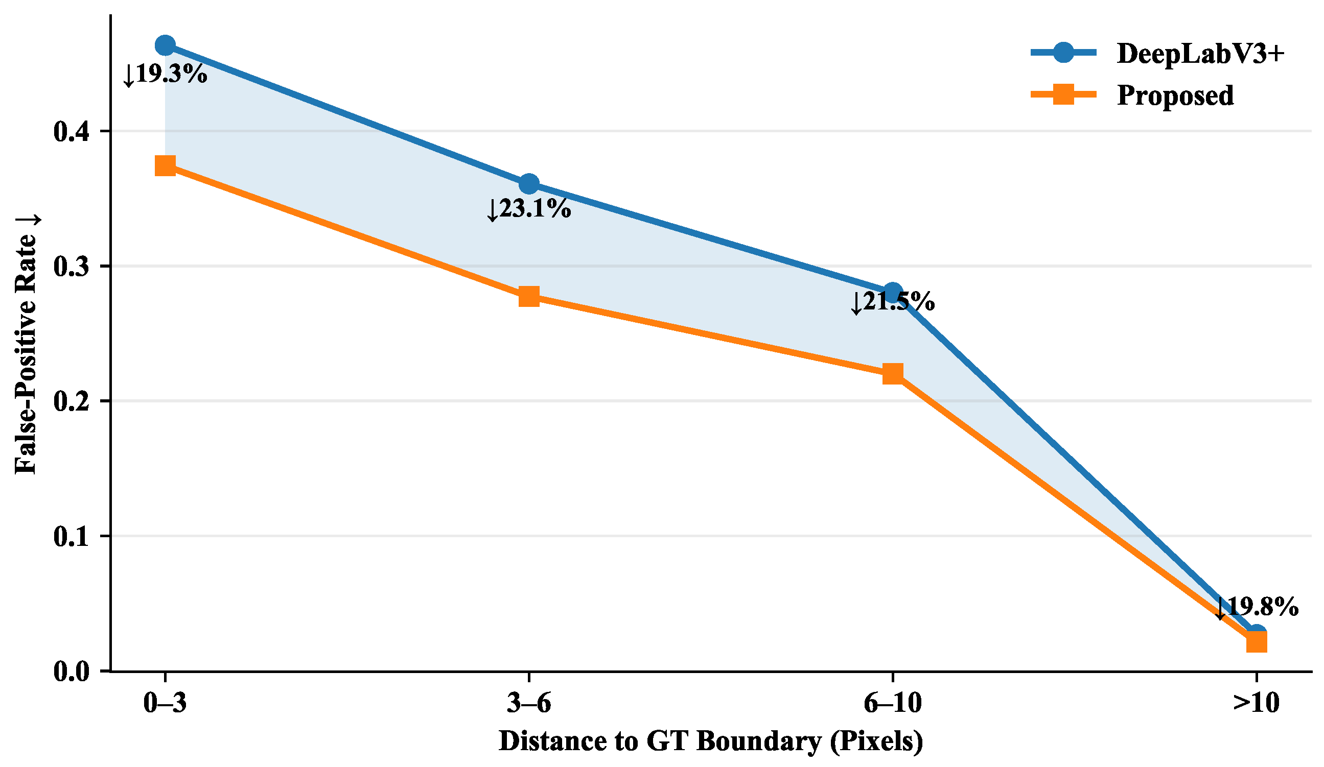
To examine whether false positives are suppressed beyond the immediate boundary region, we compute the false-positive rate of background pixels in different distance bins. Since this metric measures the proportion of true background pixels incorrectly predicted as foreground, lower values indicate stronger false-positive suppression.

As shown in Figure 5, the proposed method consistently reduces false positives across different distance bins. The reductions in near-boundary bins indicate that the method alleviates boundary over-expansion, which is consistent with the improvement in SD_3px. More importantly, the reductions in farther background bins show that the model also suppresses erroneous foreground activations in stable background regions, which explains the improvement in Precision. This result directly supports the design of FPL: instead of globally penalizing uncertain foreground responses, FPL focuses on non-boundary background regions where high foreground confidence is more likely to indicate a false positive.

4.9. Computational Cost and Inference Speed

Table 9. Computational cost and inference speed at $512\times 512$ resolution on a single RTX 3090 GPU with batch size 1. Latency is reported as mean ± standard deviation over 100 forward passes after 20 warm-up iterations and measures network inference only.

Method	Params (M)	FLOPs (G)	Latency (ms)	FPS
DeepLabV3+	45.670	112.825	$9.484\pm 0.012$	105.4
Proposed Method	46.878	153.660	$11.392\pm 0.009$	87.8

shows that the proposed method introduces limited parameter overhead but a moderate increase in FLOPs and latency. Compared with the DeepLabV3+ baseline, the parameters increase by only 2.6%, while FLOPs and latency increase by 36.2% and 20.1%, respectively, mainly due to the MSF and BGDA modules. Nevertheless, the proposed method still achieves 11.392 ms per image, or 87.8 FPS, at $512\times 512$ resolution on a single RTX 3090 GPU. This latency is below the time budgets of both 60 FPS and 30 FPS inference, suggesting that the method remains applicable to GPU-equipped industrial inspection workstations. Moreover, the boundary band and FPL are used only during training, so no additional boundary input or auxiliary boundary prediction branch is required during deployment. It should be noted that the reported speed measures network inference only; image acquisition, data transfer, visualization, post-processing, and deployment on embedded or CPU-only platforms require further investigation.

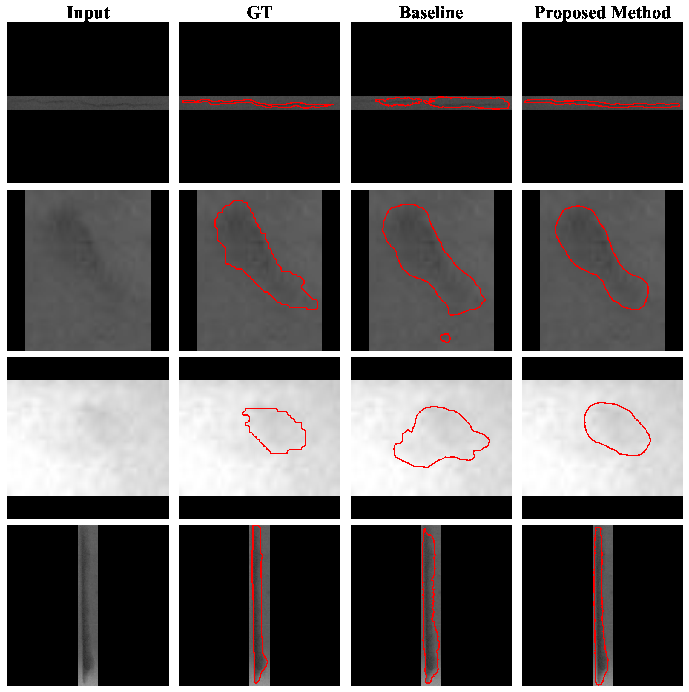
4.10. Qualitative Results

Figure 6 shows representative qualitative comparisons between the baseline and the proposed method. The selected cases include several typical segmentation challenges in weld radiographs, such as thin seam-aligned defects, low-contrast defect regions, blurred boundaries, and elongated narrow defects. In the first row, the baseline detects the main defect region but produces an over-expanded contour along the weld seam, especially on the right side of the defect. In contrast, the proposed method generates a thinner and more compact prediction that is closer to the ground-truth contour. This visual result is consistent with the improvement in Precision and SD_3px, indicating that the proposed method reduces boundary-induced foreground expansion.

In the second row, both methods roughly localize the main elongated defect, but the baseline introduces an isolated false-positive region below the defect. The proposed method removes this isolated background activation while preserving the main defect structure. This observation directly reflects the role of FPL, which penalizes overconfident foreground responses in stable non-boundary background regions. Therefore, the qualitative result supports the quantitative increase in Precision reported in Table 2 and Table 4.

The third row illustrates a small low-contrast defect with an ambiguous boundary. The baseline produces a larger and more irregular prediction, suggesting that weak grayscale transitions can easily lead to over-segmentation. The proposed method yields a more compact contour and suppresses surrounding background responses. Although some fine contour irregularities are smoothed, the overall prediction is closer to the defect extent and avoids excessive foreground expansion. This result suggests that BGDA helps regularize boundary-sensitive feature refinement rather than simply amplifying all weak responses.

The fourth row further shows the advantage of the proposed method for a long and narrow defect. The baseline prediction is relatively irregular and slightly expanded along the defect boundary, whereas the proposed method maintains a more continuous and narrower contour. This indicates that MSF helps retain weak elongated defect responses, while BGDA constrains the refined features around boundary-adjacent regions. Overall, the qualitative comparisons show that the proposed method improves segmentation quality mainly by reducing over-expanded contours and isolated false positives while preserving the main defect regions. These visual patterns explain why the proposed method achieves higher Dice, Precision, and SD_3px without relying on excessive foreground expansion.

5. Conclusions

This study investigates pixel-level weld radiographic defect segmentation, a relatively underexplored yet important task for automated non-destructive testing and quantitative weld-quality assessment. To address the challenges of weak defect boundaries, foreground–background imbalance, and defect-like background responses, we proposed a boundary-guided feature modulation framework with false-positive suppression. The proposed framework integrates multi-scale feature fusion, boundary-guided dual attention, and a false-positive suppression loss to jointly improve weak defect recovery, boundary localization, and background cleanliness. The boundary band is constructed from training annotations and is used only as a label-derived training-time regularization signal; during validation and testing, the model requires only the input radiograph and does not use any ground-truth mask, boundary band, or predicted boundary map.

Experimental results on a real-world industrial weld radiographic dataset demonstrate that the proposed method achieves better overall segmentation performance than representative CNN-based and Transformer-based baselines. In particular, the proposed method achieves a Dice score of $0.810\pm 0.003$, a Precision of $0.809\pm 0.004$, and a Surface Dice at 3 pixels of $0.394\pm 0.008$. Compared with conventional segmentation models, the proposed method produces more accurate defect masks, improves precision and boundary alignment, and effectively reduces false-positive activations in stable background regions while maintaining competitive recall. Image-wise paired statistical significance analysis further confirms that the main improvements in Dice, Precision, and SD_3px are statistically meaningful after multiple-comparison correction. The ablation study, loss comparison, qualitative visualization, and distance-based false-positive analysis further show that the performance gains are methodologically consistent with the proposed design: MSF helps recover weak defect responses, BGDA improves boundary-sensitive feature refinement, and FPL suppresses foreground leakage above a tolerated confidence margin in stable non-boundary background regions.

Despite these improvements, this study still has several limitations. First, the dataset was collected from an industrial inspection project and cannot be fully released because of confidentiality restrictions. This proprietary nature inherently limits direct external reproducibility. To partially mitigate this limitation and facilitate future research, we have made the source code publicly available at https://github.com/Xe7naga/BGDA (accessed on 20 June 2026) and provided comprehensive implementation details, enabling the community to readily apply and evaluate the proposed framework on their own datasets. Second, although the dataset contains diverse defect categories and imaging variations, the main experiments are still conducted on a single proprietary dataset. When applied to radiographic images acquired under different inspection procedures, equipment configurations (e.g., varying X-ray sources or exposure parameters), or industrial sectors, the images may exhibit significant domain shifts in contrast, noise levels, and weld morphology. We expect the proposed framework to maintain reasonable generalization capability for several reasons. Fundamentally, the physical manifestation of weld defects as local density variations remains consistent across different imaging setups, and the proposed multi-scale feature fusion and false-positive suppression mechanisms are specifically designed to capture these intrinsic local texture and contrast anomalies rather than overfitting to specific global image patterns. Furthermore, because the boundary guidance serves solely as a training-time regularization, it forces the network to learn robust internal feature representations without relying on external geometric priors during inference. This inherent independence from specific weld shapes or boundary configurations makes the model more resilient to morphological variations in cross-domain scenarios. Nevertheless, for scenarios with extreme distribution shifts, external validation on cross-domain datasets remains necessary, and techniques such as domain adaptation or lightweight fine-tuning may be required to further optimize performance. Third, extremely low-contrast defects, very thin elongated defects, and cases with severe defect-like background textures remain challenging. Future work will focus on cross-domain validation, multi-class weld defect segmentation, adaptive boundary modeling under more diverse imaging conditions, and practical deployment studies in industrial NDT workflows.

References

1. Wang, X.; Zscherpel, U.; Tripicchio, P.; D’Avella, S.; Zhang, B.; Wu, J.; Liang, Z.; Zhou, S.; Yu, X. A Comprehensive Review of Welding Defect Recognition from X-ray Images. J. Manuf. Process. 2025, 140, 161–180. [Google Scholar] [CrossRef] [Scilit]
2. Zhao, X.; Wu, J.; Zhang, B.; Wen, H.; Wang, X.; Li, Y.; Yu, X. SWRD: A Dataset of Radiographic Image of Seam Weld for Defect Detection. J. Nondestruct. Eval. 2024, 44, 50. [Google Scholar] [CrossRef] [Scilit] [PubMed]
3. Xu, H.; Yan, Z.; Ji, B.; Huang, P.; Cheng, J.; Wu, X. Defect Detection in Welding Radiographic Images Based on Semantic Segmentation Methods. Measurement 2022, 188, 110569. [Google Scholar] [CrossRef] [Scilit]
4. Elhendawy, G.A.; El-Taybany, Y. Machine Vision-Assisted Welding Defect Detection System with Convolutional Neural Networks. Int. J. Precis. Eng. Manuf. 2025, 26, 3185–3194. [Google Scholar] [CrossRef] [Scilit]
5. Wang, X.; He, F.; Huang, X. A New Method for Deep Learning Detection of Defects in X-ray Images of Pressure Vessel Welds. Sci. Rep. 2024, 14, 6312. [Google Scholar] [CrossRef] [Scilit] [PubMed]
6. Wang, Q.; Mei, J.; Jiang, W.; Zhu, H. SHDM-NET: Heat Map Detail Guidance with Image Matting for Industrial Weld Semantic Segmentation Network. Eng. Appl. Artif. Intell. 2023, 126, 106946. [Google Scholar] [CrossRef] [Scilit]
7. Zhang, B.; Wang, X.; Cui, J.; Wu, J.; Wang, X.; Li, Y.; Li, J.; Tan, Y.; Chen, X.; Wu, W.; et al. Welding Defects Classification by Weakly Supervised Semantic Segmentation. NDT E Int. 2023, 138, 102899. [Google Scholar] [CrossRef] [Scilit]
8. Yan, Z.; Ji, B.; Xu, H.; Fang, J. Interactive Defect Segmentation in Welding Radiographic Images Based on Artificial Features Fusion. NDT E Int. 2025, 151, 103305. [Google Scholar] [CrossRef] [Scilit]
9. Hu, M.; Hu, X.; Zhao, J.; Zhan, H. Weld Seam ROI Detection and Segmentation Method Based on Active–Passive Vision Fusion. Sensors 2025, 25, 7530. [Google Scholar] [CrossRef] [Scilit] [PubMed]
10. Ronneberger, O.; Fischer, P.; Brox, T. U-Net: Convolutional Networks for Biomedical Image Segmentation. In Medical Image Computing and Computer-Assisted Intervention–MICCAI 2015; Lecture Notes in Computer Science; Navab, N., Hornegger, J., Wells, W., Frangi, A., Eds.; Springer: Cham, Switzerland, 2015; Volume 9351. [Google Scholar] [CrossRef] [Scilit]
11. Chen, L.C.; Zhu, Y.; Papandreou, G.; Schroff, F.; Adam, H. Encoder-Decoder with Atrous Separable Convolution for Semantic Image Segmentation. In Computer Vision–ECCV 2018. ECCV 2018; Lecture Notes in Computer Science; Ferrari, V., Hebert, M., Sminchisescu, C., Weiss, Y., Eds.; Springer: Cham, Switzerland, 2018; Volume 11211. [Google Scholar] [CrossRef] [Scilit]
12. Wang, X.; Zhang, B.; Cui, J.; Wu, J.; Li, Y.; Li, J.; Tan, Y.; Chen, X.; Wu, W.; Yu, X. Image Analysis of the Automatic Welding Defects Detection Based on Deep Learning. J. Nondestruct. Eval. 2023, 42, 82. [Google Scholar] [CrossRef] [Scilit]
13. Urrea, C.; Vélez, M. Advances in Deep Learning for Semantic Segmentation of Low-Contrast Images: A Systematic Review of Methods, Challenges, and Future Directions. Sensors 2025, 25, 2043. [Google Scholar] [CrossRef] [Scilit] [PubMed]
14. Radi, D.; Abo-Elsoud, M.E.A.; Khalifa, F. Accurate Segmentation of Weld Defects with Horizontal Shapes. NDT E Int. 2022, 126, 102599. [Google Scholar] [CrossRef] [Scilit]
15. Zhou, Z.; Siddiquee, M.M.R.; Tajbakhsh, N.; Liang, J. UNet++: Redesigning Skip Connections to Exploit Multiscale Features in Image Segmentation. IEEE Trans. Med. Imaging 2019, 39, 1856–1867. [Google Scholar] [CrossRef] [Scilit] [PubMed]
16. Oktay, O.; Schlemper, J.; Folgoc, L.L.; Lee, M.; Heinrich, M.; Misawa, K.; Mori, K.; McDonagh, S.; Hammerla, N.Y.; Kainz, B.; et al. Attention U-Net: Learning Where to Look for the Pancreas. arXiv 2018, arXiv:1804.03999. [Google Scholar] [CrossRef] [Scilit]
17. Huang, H.; Lin, L.; Tong, R.; Hu, H.; Zhang, Q.; Iwamoto, Y.; Han, X.; Chen, Y.W.; Wu, J. UNet 3+: A Full-Scale Connected UNet for Medical Image Segmentation. In ICASSP 2020—2020 IEEE International Conference on Acoustics, Speech and Signal Processing (ICASSP); IEEE: Piscataway, NJ, USA, 2020. [Google Scholar]
18. Cao, H.; Wang, Y.; Chen, J.; Jiang, D.; Zhang, X.; Tian, Q.; Wang, M. Swin-Unet: Unet-like Pure Transformer for Medical Image Segmentation. In Computer Vision–ECCV 2022 Workshops. ECCV 2022; Lecture Notes in Computer Science; Karlinsky, L., Michaeli, T., Nishino, K., Eds.; Springer: Cham, Switzerland, 2022; Volume 13803. [Google Scholar] [CrossRef] [Scilit]
19. Xie, E.; Wang, W.; Yu, Z.; Anandkumar, A.; Alvarez, J.M.; Luo, P. SegFormer: Simple and Efficient Design for Semantic Segmentation with Transformers. arXiv 2021, arXiv:2105.15203. [Google Scholar] [CrossRef] [Scilit]
20. Ranftl, R.; Bochkovskiy, A.; Koltun, V. Vision Transformers for Dense Prediction. In 2021 IEEE/CVF International Conference on Computer Vision (ICCV); IEEE: Piscataway, NJ, USA, 2021. [Google Scholar]
21. Takikawa, T.; Acuna, D.; Jampani, V.; Fidler, S. Gated-SCNN: Gated Shape CNNs for Semantic Segmentation. arXiv 2019, arXiv:1907.05740. [Google Scholar] [CrossRef] [Scilit]
22. Marmanis, D.; Schindler, K.; Wegner, J.D.; Galliani, S.; Datcu, M.; Stilla, U. Classification With an Edge: Improving Semantic Image Segmentation with Boundary Detection. ISPRS J. Photogramm. Remote Sens. 2018, 135, 158–172. [Google Scholar] [CrossRef] [Scilit]
23. Ishikawa, H.; Aoki, Y. Boosting Semantic Segmentation with Semantic Boundaries. arXiv 2023, arXiv:2304.09427. [Google Scholar] [CrossRef] [Scilit]
24. Fu, J.; Liu, J.; Tian, H.; Li, Y.; Bao, Y.; Fang, Z.; Lu, H. Dual Attention Network for Scene Segmentation. In 2019 IEEE/CVF Conference on Computer Vision and Pattern Recognition (CVPR); IEEE: Piscataway, NJ, USA, 2019. [Google Scholar]
25. Wang, C.; Zhang, Y.; Cui, M.; Ren, P.; Yang, Y.; Xie, X.; Hua, X.S.; Bao, H.; Xu, W. Active Boundary Loss for Semantic Segmentation. Proc. AAAI Conf. Artif. Intell. 2022, 36, 2397–2405. [Google Scholar] [CrossRef] [Scilit]
26. Lin, T.Y.; Goyal, P.; Girshick, R.; He, K.; Dollár, P. Focal Loss for Dense Object Detection. arXiv 2018, arXiv:1708.02002. [Google Scholar] [CrossRef] [Scilit]
Figure 1. Overview of the proposed framework and representative qualitative comparison. (a) The proposed framework integrates multi-scale feature fusion (MSF), boundary-guided dual attention (BGDA), and false-positive suppression loss for boundary-aware weld defect segmentation. Boundary priors are used only during training, while inference requires only the input radiograph. (b) Qualitative comparison on a representative weld radiograph. Red contours denote the boundaries extracted from the ground-truth or predicted masks in the corresponding columns. The baseline model exhibits boundary over-expansion, whereas the proposed method produces a tighter contour and cleaner background prediction.
Applsci 16 06579 g001
Figure 2. Illustration of the boundary-band construction. A thin ground-truth boundary is dilated to form a narrow uncertainty band around the defect contour. The red contours visualize the extracted thin ground-truth boundary and its dilated boundary band.
Applsci 16 06579 g002
Figure 3. The proposed BGDA module. The module consists of channel attention, spatial attention, and SDR. During training, SDR uses the boundary band as a training-time prior to gate residual attention terms in both channel and spatial branches. During inference, the training-time boundary prior is not used, and the learned attention descriptors perform boundary-free residual refinement.
Applsci 16 06579 g003
Figure 4. Representative radiographic examples and corresponding pixel-level annotation masks of the seven defect categories in the weld radiographic dataset. Each column shows one defect category, where the upper row presents a cropped weld radiograph and the lower row presents the corresponding ground-truth mask. White regions in the masks denote annotated defect pixels. Columns (ag) correspond to Crack, Undercut, Porosity, Slag inclusion, Lack of fusion, Incomplete penetration, and Concavity, respectively.
Applsci 16 06579 g004
Figure 5. Distance-based false-positive analysis. Background pixels are grouped by their distance to the ground-truth boundary, and the false-positive rate is computed for each distance bin. Since this metric measures erroneous foreground predictions on true background pixels, lower values indicate better false-positive suppression. In the plot, the shaded region highlights the performance gap in false-positive rates between DeepLabV3+ and the proposed method, while the arrows and annotated percentages indicate the relative reductions achieved by our method. The proposed method consistently achieves lower false-positive rates across all bins.
Applsci 16 06579 g005
Figure 6. Qualitative comparison with DeepLabV3+. Red contours are overlaid only for visualization. In the GT column, the red contours denote the boundaries extracted from the manually annotated ground-truth defect masks. In the Baseline and Proposed Method columns, the red contours denote the boundaries extracted from the corresponding predicted binary masks after thresholding at 0.5. These contours are automatically extracted from the complete binary masks and are not manually selected local regions. The examples are selected to represent challenging cases with weak boundaries, low contrast, thin or elongated defects, and defect-like background textures. All quantitative metrics are computed on the complete test set rather than on these representative examples only.
Applsci 16 06579 g006