A Physics-Based Deep Learning Approach for Estimating Mechanical Properties of Layered Media Using Seismograms

Abstract

This research proposes a physics-based deep learning framework, developed as a proof-of-concept based on synthetic data, for estimating the mechanical properties of layered media—namely density (ρ), Young’s modulus (E), and top layer thickness (h₁)—using synthetic seismogram images generated via Finite Element Method (FEM) simulations. The dataset, comprising 5000 simulations, incorporates physical constraints and empirical density–modulus correlations. While a ResNet-style Convolutional Neural Network (CNN) extracts density and stiffness parameters from composite time–frequency images, the estimation of h1 utilizes a direct time-domain raw-signal approach to preserve spatial resolution. A 5-fold nested cross-validation scheme with internal Bayesian Optimization ensures rigorous model evaluation, further validated by normality assessments and bootstrap confidence intervals. Performance was tested against synthetic Gaussian noise (0% to 50%) and benchmarked against classical Full Waveform Inversion (FWI). The results demonstrate high predictive accuracy for shallow properties, with R² values reaching 0.96 for Young’s modulus and 0.83 for raw-signal thickness. The neural network model requires 0.035 s per inference compared to 180 s for the FWI approach, avoiding the local minima convergence issues typical of iterative inversion. The framework exhibits resilience under moderate noise levels (up to 30%), establishing a reliable baseline for future experimental validation.

1. Introduction

The profound knowledge of the physical and mechanical properties of the geological substrate is of paramount importance and unquestionable utility in any civil engineering, agricultural, or environmental undertaking [1]. Traditionally, estimating these geomaterial characteristics was an arduous and time-consuming process, relying on methodologies that often do not align perfectly with field reality or exhibit limited predictive capabilities [2]. Conventional approaches encompass a wide range of techniques, including (i) in situ tests and surveys (such as geophysical campaigns, various penetration tests, drilling and seismic tests, plate load tests, piezometers, inclinometers, extensometers, load cells, permeability tests, gravimetry, visible to near-infrared and mid-infrared spectroscopy, and magnetometry), (ii) laboratory tests, (iii) empirical relations, and (iv) numerical methods [3,4,5]. While well-established, these conventional methods face considerable challenges in modeling the complex nonlinearity inherent in geomaterial properties and the uncertainty arising from scarce data, often demanding significant computational resources.

In this context, machine learning (ML) methodologies emerge as a powerful alternative. Unlike traditional methods, which struggle with nonlinearity and complex interdependencies, ML approaches excel in discovering accurate and reliable nonlinear relationships between input variables and the geomaterial properties under study [6]. In recent decades, ML has revolutionized countless domains of human activity—from healthcare and finance to transportation and entertainment—demonstrating its eclectic applicability by finding innovative and versatile solutions for complex and continuously evolving challenges. In civil engineering, ML has catalyzed greater efficiency, accuracy, and safety, with applications ranging from analysis and design, project and construction management, geotechnical engineering, infrastructure maintenance and monitoring, materials research and development, traffic and transportation, and seismic analysis [7,8,9].

Regarding the specific focus of this research, it is pertinent to note that ML methods have successfully integrated vibration analysis across various civil engineering domains. Notable examples include evaluating the behavior and response of architectural structures or detecting damages and defects in these structures by triggering alerts when a significant difference between safety limits and real behavior is verified [10,11]. Geotechnical engineering, in particular, has benefited immensely from ML algorithms to predict soil and rock properties [12,13], map earthquake hazards [14], enhance foundation design [15], estimate settlements and bearing capacities [16], forecast slope stability issues [17], or assess liquefaction potential [18], to name just a few of the many applications of ML methodologies in this field.

Subsurface characterization, while being indispensable for site evaluation, represents an exceptionally difficult challenge in geotechnical practice. Geological processes are intrinsically complex and varied in space and time, culminating in unique scenarios with singular spatial variability in geomaterials. These, in turn, exhibit specific properties highly dependent on local conditions and geological history [19]. All these difficulties are further amplified by the necessity to interpolate material properties from scarce data, significantly increasing the uncertainty of traditional estimations. Fortunately, as the concept of big data transforms nearly every field of knowledge, geosciences have also benefited from this trend, allowing for the exploitation of spatial–temporal correlations (Tobler’s First Law of Geography) [20] and the inherent high dimensionality of geoscience data, which contain a vast number of potentially codependent variables. Deep learning (DL) architectures, such as Convolutional Neural Networks (CNNs), are particularly effective at exploiting these spatial–temporal correlations and automatically extracting hierarchical features from high-dimensional geoscience data with numerous interdependent variables [21].

Deep learning algorithms are widely applied in seismology to classify seismic events based on their type (e.g., natural earthquakes or human-induced explosions) and characteristics (e.g., local or distant events) [22]. In particular, the development of automatic recognition systems for volcanic microearthquakes is of extreme importance and utility, with the ultimate goal of correctly identifying imminent devastating eruptions, thereby enhancing data-driven decision-making processes and enabling timely, well-founded risk assessments to mitigate potential disasters. Wang and Teng [23] developed one of the earliest AI-based detectors, utilizing 50 waveforms to train Artificial Neural Networks (ANNs) with spectrograms as input. Since then, AI-based techniques have evolved for earthquake detection from scanned images of analog seismograms [24] or even from smartphone data [25] and acoustic sensing [22,26].

In recent years, the intersection of deep learning and computational mechanics has led to significant advances in physics-informed and physics-guided approaches for wave propagation and inverse problems. Among these, Physics-Informed Neural Networks (PINNs) have emerged as a prominent framework in which governing partial differential equations are incorporated directly into the training objective through residual-based constraints. Such methods have been successfully applied to wave propagation modeling and elastic-wave inversion problems, demonstrating their ability to incorporate physical knowledge into data-driven learning schemes under limited or noisy observations.

In parallel with these developments, alternative physics-guided strategies have also been explored, where physical consistency is introduced outside the optimization loop, typically during data generation or simulation stages. In this work, we adopt this latter perspective. Specifically, physically consistent wavefields are generated using finite element simulations constrained by realistic geomechanical parameter ranges and wave propagation physics. The resulting dataset is then used to train a Convolutional Neural Network for rapid inversion, without requiring the evaluation of governing equation residuals during training [27,28,29].

In an innovative approach aimed at overcoming the limitations of traditional methodologies, this research introduces a physics-based deep learning framework for predicting the physical and mechanical properties of layered media, specifically density, Young’s modulus, and top layer thickness. Unlike traditional data-driven inversion methods that operate purely on statistical correlations, the proposed physics-based deep learning framework offers distinct advantages in terms of robust optimization, physical consistency, and interpretability. A major bottleneck in classical iterative Full Waveform Inversion (FWI) is its significant vulnerability to local minima convergence, which frequently yields distorted subsurface profiles when initialized far from the true solution. The architecture developed herein bypasses this optimization pitfall through instantaneous neural mapping while explicitly embedding physical constraints into the learning pipeline. By incorporating empirical density–modulus correlations and physical velocity filters during data generation, the model is strictly bound to physically plausible parameter spaces, preventing the network from mapping arbitrary or physically impossible signal features to material properties.

This framework transitions from a theoretical model to a practical tool through a non-invasive protocol designed for geotechnical site characterization. The process involves a linear array of surface sensors designed to capture the wave propagation across the medium generated by a controlled transient point load.

Once the vertical displacement signals are collected, they are processed through two distinct pipelines. For the estimation of density and Young’s modulus, the signals are converted into velocity and merged into composite grayscale seismogram images integrating temporal and spectral features. Simultaneously, the framework utilizes the raw vertical displacement signals directly in the time domain to resolve the first layer’s thickness. This specific adaptation is necessitated by the fact that the 128 × 128 pixel resolution of the composite seismograms introduces pixelation that abstracts precise wave transit times. Initial evaluations using image-based CNNs to predict h1 resulted in insufficient accuracy, yielding absolute errors of approximately 4 m and an MAPE of 45%. By processing the raw signals, the framework preserves the temporal cues strictly necessary for accurate spatial resolution.

A ResNet-style CNN processes the images, while a specifically adapted architecture handles the raw-signal matrices to perform an instantaneous inversion of the soil properties. This automated workflow allows for the rapid estimation of soil properties while avoiding the local minima convergence issues typical of classical iterative inversion, performing inferences approximately five thousand times faster than traditional methods. To assess the robustness of the methodology, synthetic seismograms are subjected to varying levels of Gaussian noise, ranging from 0% to 50% of the pure signal’s standard deviation, prior to the training of the CNN models. Model performance is evaluated using metrics such as RMSE, MAE, R², MAPE, and R, supported by statistical validation encompassing normality assessments and 95% bootstrap confidence intervals.

This study is organized as follows: Section 1 provides an overview of recent developments in the research field; Section 2 details the development of the numerical model in MATLAB and the creation of synthetic seismogram datasets, addressing the boundary conditions and damping layer implementation within the FEM model; Section 3 presents the architecture of the CNN models, training methodology, and hyperparameter optimization; Section 4 presents the performance metrics and statistical analyses; and, finally, Section 5 presents the main conclusions and outlines avenues for future research.

2. Numerical Method

The Finite Element Method (FEM) stands as a robust numerical technique widely employed in engineering to address complex problems, particularly those involving structural dynamics and wave propagation [30]. In essence, the FEM discretizes a continuous domain into smaller, simpler elements—lineal triangles in this study—connected at nodal points where the governing equations of physics are approximated using interpolation functions. This method computes the stiffness (K), mass (M), and damping (C) matrices that describe the system’s dynamic behavior. The time-dependent solution is typically found using a time integration method, such as Newmark-beta or central difference, to calculate nodal displacements and velocities over time [31,32,33].

In this research, a dedicated FEM model was developed in MATLAB (version R2024b), building upon the foundational numerical model established by Albino et al. [34]. Although the finite element model employs a 2D configuration to enable the efficient generation of a vast dataset, the inherent limitations of this approach are acknowledged, namely its inability to capture the full complexity of 3D wave propagation.

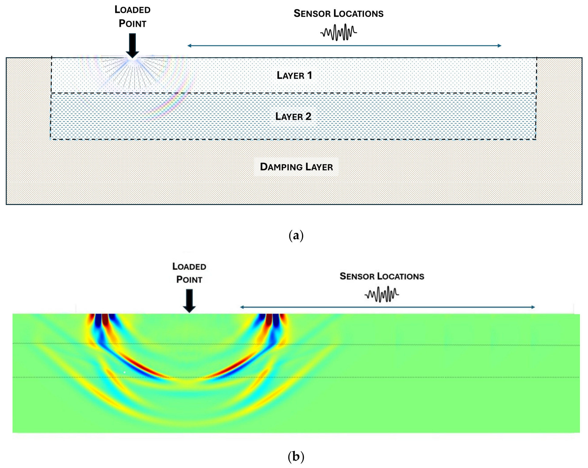
Figure 1 illustrates the schematic of the numerical model, comprising a two-layer soil profile of homogeneous materials with variable thicknesses. It should be noted that the underlying damping layer serves solely as an absorbing boundary condition, rather than a third physical stratum. To capture the propagating wavefield, a linear array of 10 surface receivers was implemented with a constant spacing of 3 m, starting at a distance of 10 m from the dynamic excitation source.

To ensure that the simulated material properties explore a realistic parameter space mimicking superficial geotechnical formations, an empirical relation established by Choi et al. (2020) [35] was adopted as a baseline. This relation links dry density (γ_d, in kN/m³) to the soil stiffness modulus (E, in MPa), as defined by Equation (1):

$$E=14.13{\gamma }_d-180.63$$

(1)

To cover a broad spectrum of shallow geomaterials, ranging from loose silts and soft clays to compacted granular layers, the targeted parameters were sampled across wider independent ranges, constraining mass density (ρ) between 1350 and 2040 kg/m³ and Young’s modulus (E) between 10 and 150 MPa. To avoid introducing rigid mathematical dependencies that do not reflect field heterogeneity, independent random sampling was introduced via a continuous stochastic perturbation factor varying uniformly between 0.7 and 1.3. This randomized ±30% scaling was applied directly during database generation (E = E_baseline × [0.7 + 0.6 × rand]).

This stochastic scattering decouples the strict functional link between the two physical properties, ensuring that the deep learning framework is trained on overlapping parameter distributions rather than an artificial deterministic formula, thus mirroring the natural physical scatter observed in empirical geotechnical prospecting. The relevant parameters and limit variation ranges for the FEM simulation are presented in

Table 1. Relevant parameters and limit variation ranges for the FEM simulation.

GEOMETRIC PARAMETERS
Parameter	Limit values
Thickness of Layer 1	[1 to 10] m
ELASTIC PARAMETERS
Parameter	Limit values
Young’s modulus (E)	[10 to 150] MPa
Poisson coefficient (µ)	[0.27 to 0.37]
PHYSICAL PARAMETERS
Parameter	Limit values
Density (ρ)	[1350 to 2040] kg/m3

.

To ensure a representative exploration of the parameter space, a uniform random sampling strategy was adopted. This approach enabled the generation of a diverse dataset of 5000 simulations, providing sufficient variability and coverage for training the deep learning models and enhancing their ability to generalize to unseen cases. Specifically, the generated database compiles the target geotechnical properties for each modeled layer alongside the resulting dynamic response—namely, the temporal evolution of vertical displacements at the 10 surface receivers. These synthetic seismograms constitute the raw input features that are subsequently processed into the time–frequency images and signal matrices used by the deep learning models.

3. Machine Learning

In the realm of civil and geotechnical engineering, traditional methods for characterizing subsurface properties often involve expensive and time-consuming in situ and laboratory tests or computationally intensive numerical simulations that frequently struggle to fully account for the inherent complexities and well-established nonlinear behavior of geomaterial properties across diverse geological conditions. As discussed by Pitilakis et al. [2] and Liu et al. [19], these conventional approaches face significant challenges in modeling the nonlinearity inherent in geomaterials.

Machine learning offers an effective alternative by discovering accurate and reliable nonlinear relationships within high-dimensional and interdependent datasets. According to Kohestani and Hassanlourad [6], these algorithms excel in finding innovative solutions to complex and continuously evolving challenges. The capacity of these methods has been significantly enhanced by advances in technology and computational infrastructure, allowing for the identification of intricate patterns in large-scale datasets such as the 5000 FEM-generated simulations used in this study. This approach plays a crucial role in predicting material properties, as demonstrated by Thai [36], Ercins [37], and Stergiou et al. [38]. Deep learning architectures, specifically Convolutional Neural Networks, are particularly adept at exploiting spatial–temporal correlations and automatically extracting hierarchical features from high-dimensional geoscience data. As highlighted by Karpatne et al. [21] and Mousavi and Beroza [22], these networks are essential for processing the complex signals typical of subsurface characterization.

3.1. Convolutional Neural Networks (CNNs)

Every computer vision system begins by capturing light reflected from an object and converting those optical signals into a digital image that a computer can process. Essentially, an image is represented as a matrix (or three matrices if color channels are separated) containing numerical values that correspond to intensity and color information [39]. CNNs are a specific type of neural network with a grid-like topology that has demonstrated remarkable success in processing image data. Among other characteristics, CNNs employ a mathematical operation called convolution, which acts as a filter to extract features from the input. This is achieved by convolving a raw signal, or image patch, with a weighing function (a kernel or filter) which assigns specific weights to neighboring values. The resulting smoothed signal, s(t), is given by Equation (2) [40]:

$$s\left(t\right)={\displaystyle \underset{-\infty }{\overset{\infty }{\int }}}h\left(a\right)v\left(t-a\right)da$$

(2)

Here, h(t) represents the raw signal and v(t) is the weighting function.

CNNs are built upon three fundamental principles: local receptive fields, weight sharing, and pooling. Unlike fully connected layers, which link every input pixel to each hidden unit—resulting in a large number of parameters—CNNs focus on small regions of the image (e.g., a 3 × 3 patch). This allows each hidden unit to learn localized features like edges or textures by computing the dot product between a filter (optimized via backpropagation) and the patch, ensuring that the network captures regional patterns rather than isolated pixel values. As these local receptive fields move across the image, they generate a feature map (essentially a matrix formed by the dot products plus a bias term). A nonlinear activation function, such as ReLU, is then applied, setting negative values to zero while retaining positive values. Pooling layers, like max-pooling (which selects the maximum value within a region), further reduce spatial dimensions by summarizing areas, making the model more resilient to small variations or shifts in the input image. This architecture not only speeds up training but also enables the construction of deep networks that excel in recognizing complex patterns [41,42]. 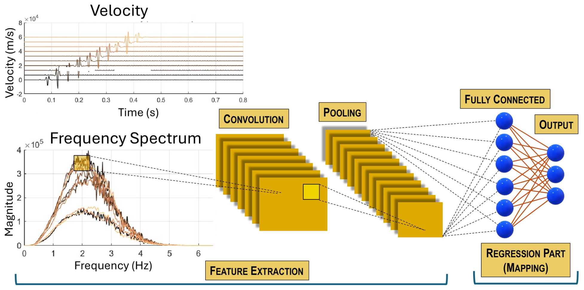Figure 2 illustrates a general representation of a CNN idealized for a regression model.

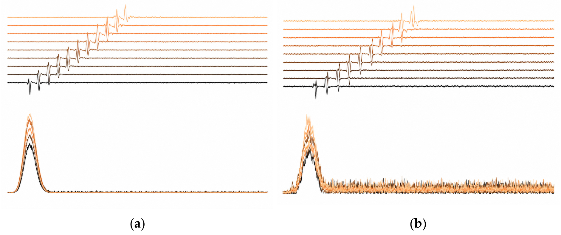
In this study, the predictive framework was implemented in MATLAB R2024b using two distinct data processing pipelines. For the estimation of density and Young’s modulus, the raw vertical movement signals from the ten surface sensors were converted into composite seismogram images. This involved calculating the velocity through time differentiation, followed by determining frequency components using Fast Fourier Transform (FFT). These temporal and spectral features were merged into single-channel grayscale images, resized to a uniform 128 × 128 pixel resolution, and normalized.

Figure 3 shows an example of these composite seismogram images.

For the estimation of h₁, the framework utilizes a direct raw-signal approach. The raw vertical displacement signals were structured into a numerical matrix of 4096 time steps by 10 sensor channels. This high-resolution matrix ensures the preservation of precise wave transit times necessary for accurate spatial resolution.

The targets were normalized using a Z-score method. For evaluation, predictions were converted back to their original physical units to ensure accurate error measurement. A 5-fold nested cross-validation method was used, ensuring zero data leakage by isolating the test set before any hyperparameter optimization.

Two distinct CNN architectures were employed. The image-based models utilized a ResNet-style architecture featuring a convolutional trunk with seven sequential blocks and skip connections. Each block includes a 2D convolutional layer (with filters increasing from 16 to 256), batch normalization, ReLU activation, and max-pooling. For the raw-signal model, a multi-input CNN architecture was developed. The primary branch processes the 4096 × 10 signal matrix through four convolutional blocks utilizing specialized [15 × 3] kernels and [4 × 1] max-pooling layers.

This branch is then concatenated with a secondary input containing the elastic meta-features (density and Young’s modulus) to provide physical context to the thickness inversion loop. To ensure methodological rigor and prevent performance overestimation, a clear distinction was maintained between the network training and testing phases within the nested cross-validation loop. During the training stage of the h₁ network, the meta-feature branch was supplied with the exact numerical ground-truth values. This approach acts as an auxiliary conditioning variable to stabilize the learning process, allowing the model to map the fundamental physical relationships between wave transit signatures and layer geometry under well-defined elastic contexts. During the independent testing and validation phase, the multi-input network was fed exclusively with the predicted parameters generated by the upstream image-based CNN models trained on that specific fold. No ground-truth material properties were available to the thickness model during evaluation. The global error metrics, standard deviations, and confidence intervals reported in Section 4 inherently incorporate the complete cascade of error propagation across the predictive pipeline. The combined features then pass through two fully connected layers (256 and 64 neurons) before the final regression output, validating that the h₁ model remains highly robust even when subjected to the degraded inputs of the prior cascaded stages. Additionally, a Random Forest (RF) regressor was implemented as a baseline for h₁ estimation. Unlike the CNN models, the RF approach relies on a vector of 70 handcrafted features extracted from the 10 sensor channels, including statistical moments (RMS, kurtosis, skewness) and Time-of-Flight (ToF) metrics. The model consists of an ensemble of 100 regression trees trained via bootstrap aggregation (Bagging), with all features sampled at each split to maximize the capture of physical correlations. To ensure comparability, the RF baseline followed the same 5-fold nested cross-validation protocol and Z-score normalization as the deep learning frameworks.

Thus, three separate CNN models were trained. For density and Young’s modulus, hyperparameters were fine-tuned using Bayesian Optimization within the inner cross-validation loop. The raw-signal convolutional model for h₁ parameter estimation utilized a fixed configuration of optimization hyperparameters, including a mini-batch size of 32, an L2 regularization factor of 1 × 10⁻⁴, and an initial learning rate of 1 × 10⁻³. This configuration was trained without an integrated Bayesian Optimization loop in order to manage the computational cost of the nested 5-fold cross-validation framework. Preliminary sensitivity analyses indicated that the model exhibits stable convergence behavior under reasonable variations in these hyperparameters, with negligible impact on validation error and consistently low mean absolute error for thickness estimation. Given this robustness, an additional automated hyperparameter optimization stage over the high-dimensional time-domain input space was not pursued due to the unfavorable computational cost–benefit trade-off.

Table 2. Optimal hyperparameters applied in the ML models when training for each target property.

Model	Hyperparameters
CNN (ρs, E)	Optimizer: Adam Max Epochs: 80 (final training) Mini Batch Size: 4 Validation Patience: Inf Initial Learn Rate: Bayesian Optimization Search [1 × 10−4, 1 × 10−2] L2 Regularization: Bayesian Optimization Search [1 × 10−5, 1 × 10−2] Learn Rate Schedule: piecewise Learn Rate Drop Period: 40 Learn Rate Drop Factor: Bayesian Optimization Search [0.1, 0.9]
Raw-Signal CNN (h1)	Optimizer: Adam Max Epochs: 80 Mini Batch Size: 32 Validation Patience: 15 Initial Learn Rate: 1 × 10−3 (fixed) L2 Regularization: Default 1 × 10−4 Learn Rate Schedule: piecewise Learn Rate Drop Period: 25 Learn Rate Drop Factor: 0.5
Baseline RF (h1)	Method: Bagging (Bootstrap Aggregation Learners: 100 Regression Trees (CART) Min Leaf Size: 1 NumVariablesToSample: 70 (All features per split) Feature Extraction: 70 Statistical/Time-of-Flight features Normalization: Z-score (Mean 0, Std 1) Cross-Validation: 5-Fold Nested CV

summarizes the final training configuration.

3.2. Statistical Metrics and Analysis

The performance of the predictive models was evaluated using a suite of standard statistical metrics, including Pearson’s correlation coefficient (R), coefficient of determination (R²), Root Mean Squared Error (RMSE), mean absolute error (MAE), and Mean Absolute Percentage Error (MAPE). All metrics were calculated after denormalizing the predictions back to their original physical units—kg/m³ for density, MPa for Young’s modulus, and meters for layer thickness—ensuring that the reported errors are directly interpretable in geotechnical terms. To guarantee the statistical significance of the results, the analysis incorporated the Lilliefors test, visually supported by Quantile–Quantile (Q-Q) plots, to assess the normality of the performance distributions. Uncertainty and model stability were quantified using bootstrap resampling with 1000 iterations to estimate 95% confidence intervals, which are represented as error bars in the consolidated performance charts. This comprehensive statistical framework ensures that the observed performance variations are solid and not the result of stochastic data partitioning.

4. Results

This section analyses the performance of the CNN models trained on the dataset of 5000 FEM simulations. The evaluation focuses on predictive accuracy, stability, and robustness under varying noise conditions. The performance metrics RMSE, MAE, R², MAPE, and R were determined through a 5-fold nested cross-validation scheme to assess the models’ capabilities across different properties and layers.

The statistical significance of these results was evaluated through a normality assessment (Lilliefors tests, supported by Quantile–Quantile plots, to evaluate the distribution of the performance metrics) and an uncertainty quantification (95% bootstrap confidence intervals, estimated via 1000 resampling iterations, to establish the stability and precision of the reported means).

While the image-based CNN accurately predicts material properties, estimating h₁ required a methodological shift. To preserve precise time-domain resolution, the methodology was adapted to process the raw signal directly. This direct approach employs a 15 × 3 scanning matrix over the time-domain data, conceptually mirroring the CNN’s spatial pixel-scanning mechanism, but explicitly retaining the raw temporal accuracy.

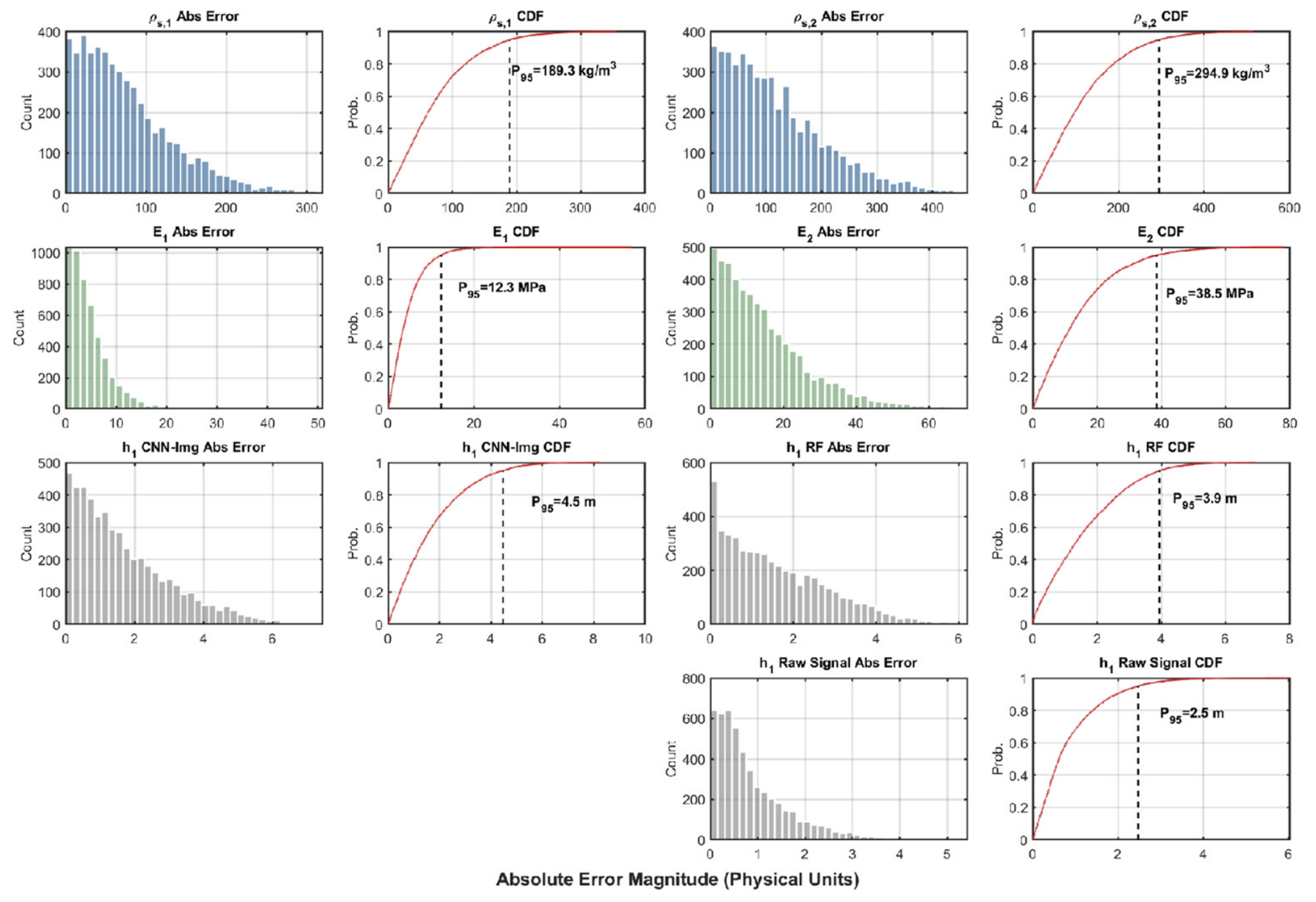
A Random Forest (RF) model was specifically included to establish a conventional machine learning baseline, demonstrating the intrinsic limitations of relying solely on classical feature-based predictions for this specific parameter. Figure 4 justifies this adaptation by presenting the absolute error histograms and Cumulative Distribution Functions (CDFs), allowing for a direct performance benchmark of the h₁ estimation across the CNN-Image, RF, and raw-signal methods.

4.1. Absolute Error Distribution and Methodological Comparison

To evaluate the predictive reliability of the trained models across the 5000 test simulations, a comprehensive analysis of the absolute error distributions was conducted. Figure 4 presents these error populations using histograms paired with their respective Cumulative Distribution Functions (CDFs). This probabilistic view highlights the 95th percentile error (P₉₅), establishing a practical confidence threshold for each parameter.

The absolute error distributions in Figure 4 demonstrate the CNN’s aptitude in extracting material properties, with error magnitudes heavily concentrated near zero. As anticipated by wave attenuation and geometric dispersion principles, predictive accuracy naturally degrades for deeper strata; the P₉₅ error increases from 189.3 to 294.9 kg/m³ for density and from 12.3 to 38.5 MPa for Young’s modulus between the first and second layers. The bottom panels empirically validate the methodological shift for estimating the first layer’s thickness (h₁). Because image-based and tabular feature extractions abstract critical wave transit times, the CNN-Image and Random Forest baseline yield higher P₉₅ errors of 4.5 m and 3.9 m, respectively. In contrast, the raw-signal approach significantly tightens the error distribution, achieving a superior P95 of 2.5 m. This maximum error boundary at the P95 level under high-noise conditions indicates that the method is not intended for high-precision geotechnical design tasks, such as final foundation dimensioning or slope stability safety analysis. Instead, the primary value of the proposed framework lies in preliminary geotechnical screening and large-scale subsurface reconnaissance. Given that the mean absolute error remains approximately 0.85 m, the model provides spatially distributed first-order estimates of h₁ suitable for mapping bedrock depth variations along extended linear infrastructures like highways, tunnels, and pipelines. In this context, the method enables rapid, non-destructive profiling and supports the optimization of subsequent high-resolution intrusive investigations, such as boreholes or Standard Penetration Tests. This places the approach within the same operational category as first-pass geophysical inversion techniques, which typically operate under comparable uncertainty levels in the absence of dense ground-truth constraints.

4.2. Evaluation Metrics—R, R², RMSE, MAE, and MAPE

This section details the quantitative performance evaluation of the ResNet-style CNN models trained on a dataset of 5000 FEM simulations. The results for R, R², RMSE, MAE, and MAPE metrics illustrate the model’s predictive capability and its variability across five independent training runs. For all performance visualizations, error bars represent the Standard Error of the Mean (SEM) calculated across the five cross-validation folds, ensuring the stability and repeatability of the learning process.

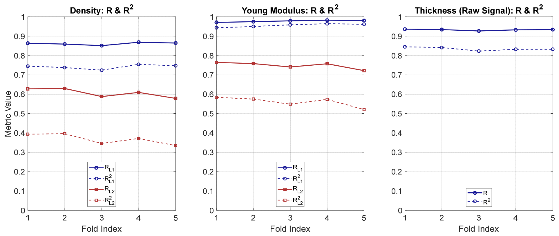
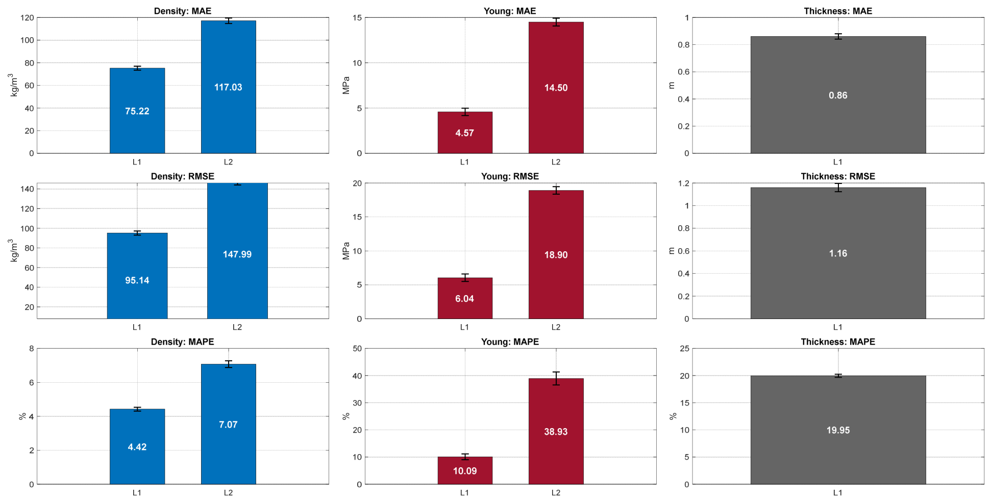
Figure 5 illustrates the correlation (R) and determination (R²) coefficients for all output parameters, presenting the evolution of R and R² metrics across the five cross-validation folds. Figure 6 and Figure 7 show the average values of RMSE, MAE, and MAPE across the independent training runs.

Figure 5 illustrates the Pearson correlation coefficient and coefficient of determination across the 5-fold cross-validation process. The results indicate strong and consistent predictive performance across all folds, with higher accuracy observed for Young’s modulus compared to density.

This difference in performance is consistent with both the data generation procedure and the underlying physics of wave propagation. Although a linear relationship between Young’s modulus and density is defined in Equation (1), a stochastic perturbation factor (0.7–1.3) was introduced during dataset generation to avoid a strictly deterministic mapping and to represent natural variability in geomechanical properties. This results in partially overlapping parameter distributions rather than an exact functional dependency.

From a physical perspective, seismic wave propagation is more sensitive to variations in elastic stiffness, which governs wave velocity and strongly influences travel time and phase characteristics. Density variations, while still relevant, have a comparatively weaker influence within the considered parameter range. This difference in sensitivity contributes to the higher predictive accuracy observed for Young’s modulus relative to density.

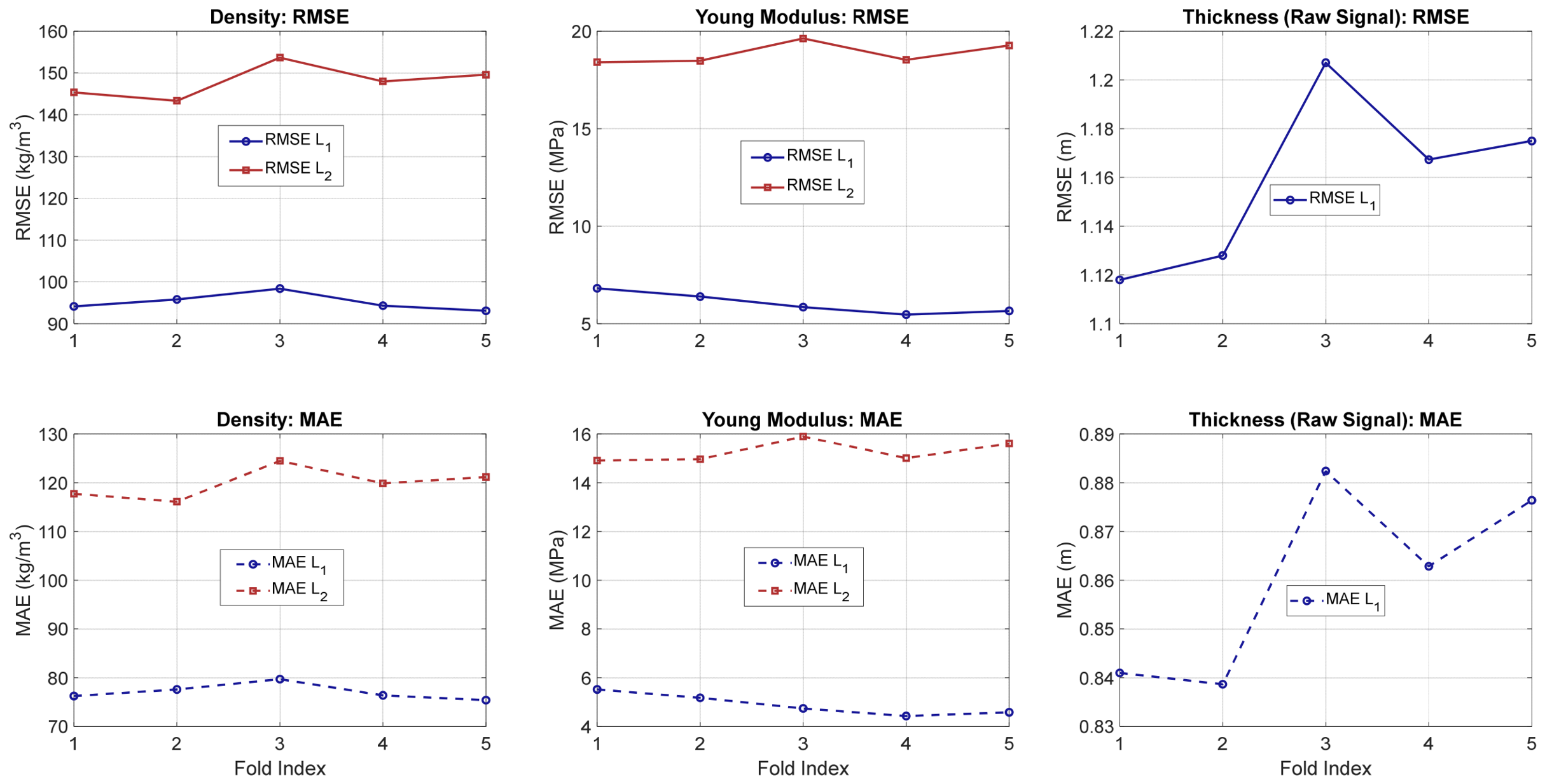
Consistent with the absolute error distributions previously discussed, predictive performance is superior for the first layer (L₁) compared to the second layer (L₂), where the observed performance degradation—with R² dropping below 0.60—reflects the combined effects of signal attenuation and geometric dispersion in deeper strata. Figure 6 shows the evolution of the RMSE and MAE metrics over the five independent training runs.

Analyzing Figure 6, and corroborating earlier statistical findings, the predictive accuracy for the first layer significantly outperforms that of the second layer. The L₁ RMSE for density and Young’s modulus remains tightly constrained beneath 100 kg/m³ and 7 MPa, respectively, whereas the L₂ errors climb to approximately 150 kg/m³ and 19 MPa. Additionally, the raw-signal methodology for estimating thickness yields a highly consistent MAE fluctuating marginally between 0.84 and 0.88 m across the folds. Again, the results demonstrate how signal attenuation and dispersion inherently reduce the resolution and predictability of deeper geological strata.

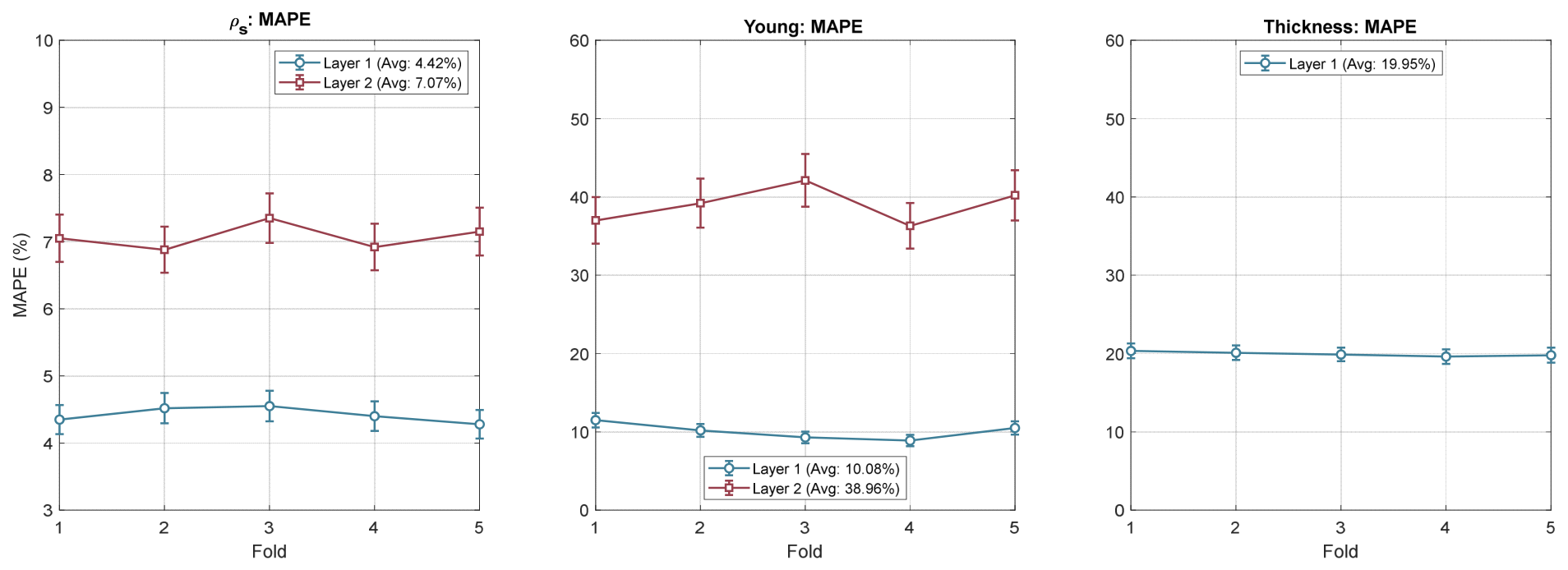
Figure 7 exhibits the solid cross-fold stability of the models. Density predictions are highly accurate, yielding a low 4.42% error for the first layer and maintaining a reliable 7.07% for the second layer. Young’s modulus estimations achieve a solid 10.08% error in L₁, before adjusting to 38.96% in L₂ as a natural physical response to expected wavefield attenuation and scattering. Coupled with a consistent 19.95% error for the raw-signal thickness (h₁) estimation, MAPE also validates the model’s overall proficiency in mapping complex material properties.

4.3. Statistical Analysis of the ML Models

This section details the statistical analysis conducted to evaluate the performance metrics of the CNN models. The primary objective was to ensure the reliability, interpretability, and statistical significance of the results presented in the previous sections.

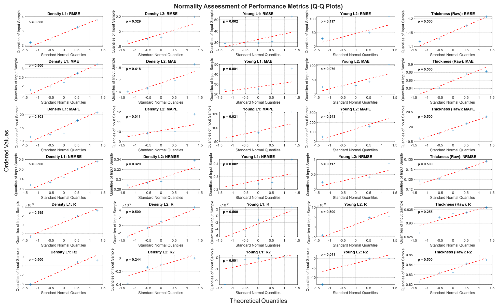
Figure 8 presents Quantile–Quantile (Q-Q) plots to assess the normality of the performance metrics across the 5-fold cross-validation framework.

To correctly interpret the data presented in Figure 9, it is important to recall that a distribution is considered normal when the majority of its values are symmetrically clustered around the mean, with fewer observations toward the extremes. Despite the inherent statistical sensitivity of hypothesis testing with a restricted sample size (N = 5 folds), the empirical quantiles predominantly align with the theoretical normal distribution references. While isolated deviations occur, yielding low p-values for specific metrics such as the first layer’s Young’s modulus, most error distributions demonstrate strong adherence to normality, frequently reaching the test’s upper confidence bound (p = 0.500). This assessment confirms the absence of extreme intra-fold biases, further substantiating the overall statistical reliability, consistency, and robustness of the training methodology.

Figure 9 and Figure 10 provide a comprehensive overview of the model’s predictive performance, displaying the mean values for key evaluation metrics: correlation coefficient (R), coefficient of determination (R²), mean absolute error (MAE), Root Mean Squared Error (RMSE), and Mean Absolute Percentage Error (MAPE).

To ensure statistical robustness and justify the presence of the error bars in these visualizations, a bootstrap resampling technique with a 95% confidence interval was applied. This method involves repeated resampling with replacement, allowing for the quantification of uncertainty and the assessment of result consistency across multiple training iterations. It demonstrates that the reported averages are stable and not biased by a specific data partition.

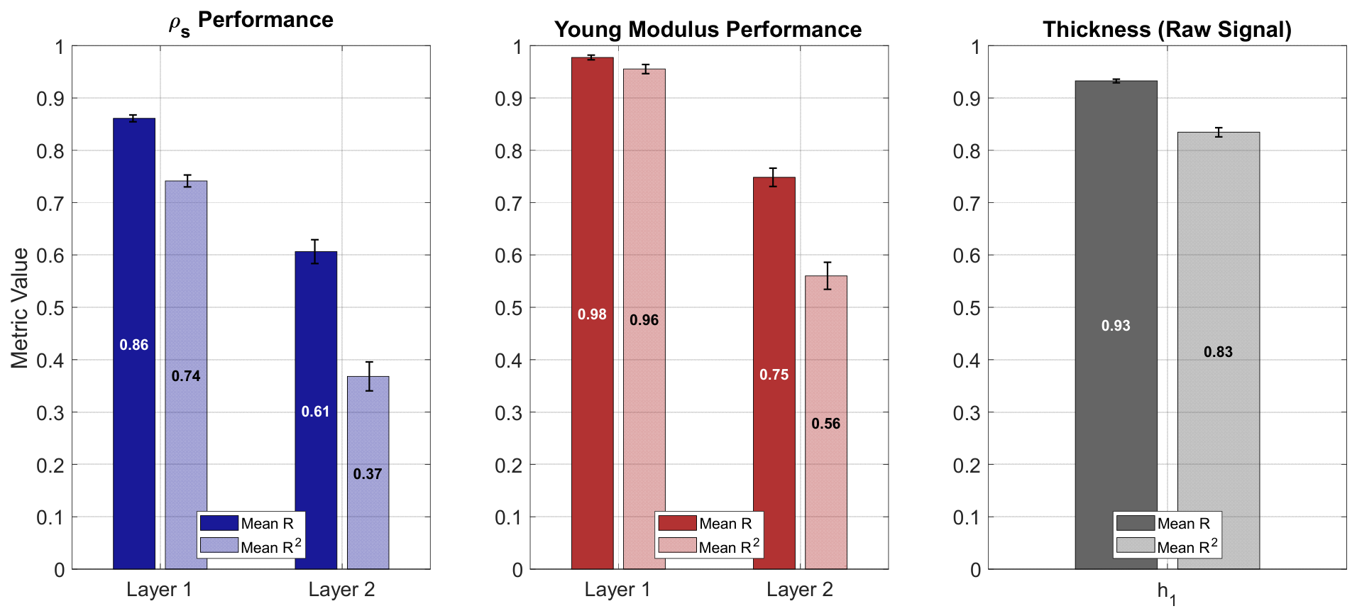
To quantify the statistical reliability of the predictive models, a bootstrapping technique was applied to compute the confidence intervals, which are represented by the narrow error bars in Figure 9. This figure displays the bootstrapped mean Pearson correlation and coefficient of determination, confirming a highly stable predictive performance across the evaluated parameters. The architecture demonstrates exceptional accuracy for surface-level characterization, achieving mean R² values of 0.96 for L₁ Young’s modulus and 0.83 for the raw-signal thickness (h₁) estimation. As physically anticipated by wavefield attenuation, the metrics naturally adjust for the deeper L₂, with density and Young’s modulus values reflecting the inherent geometric dispersion constraints of the propagating signal.

Figure 10 provides a detailed breakdown of the absolute and relative error metrics, including MAE, RMSE, and MAPE. To ensure the reliability of these performance indicators, the error bars displayed in the graphs represent the standard deviation (STD) derived from the bootstrap resampling process. This is considered to be essential to demonstrate that the model’s errors are stable across different training runs and data partitions, providing a clear measure of the precision and repeatability of the results.

Figure 10 provides a comprehensive synthesis of the mean performance metrics (MAE, RMSE, and MAPE) enhanced with bootstrapped confidence intervals. The narrow error bars across all evaluated parameters confirm the architecture’s statistical stability and high degree of reliability. The model delivers highly accurate characterizations for L1, highlighted by a minimal density MAPE of 4.42%. For the deeper L2, the performance metrics predictably adjust, such as Young’s modulus MAPE shifting to 38.93%, which accurately reflects the natural physical constraints of wavefield attenuation and geometric dispersion rather than a modeling deficit. These aggregated results validate the methodology’s proficiency in translating complex, depth-attenuated geophysical signals into reliable material profiles.

4.4. Analysis of the Noise Percentage Influence on CNN Model Performance

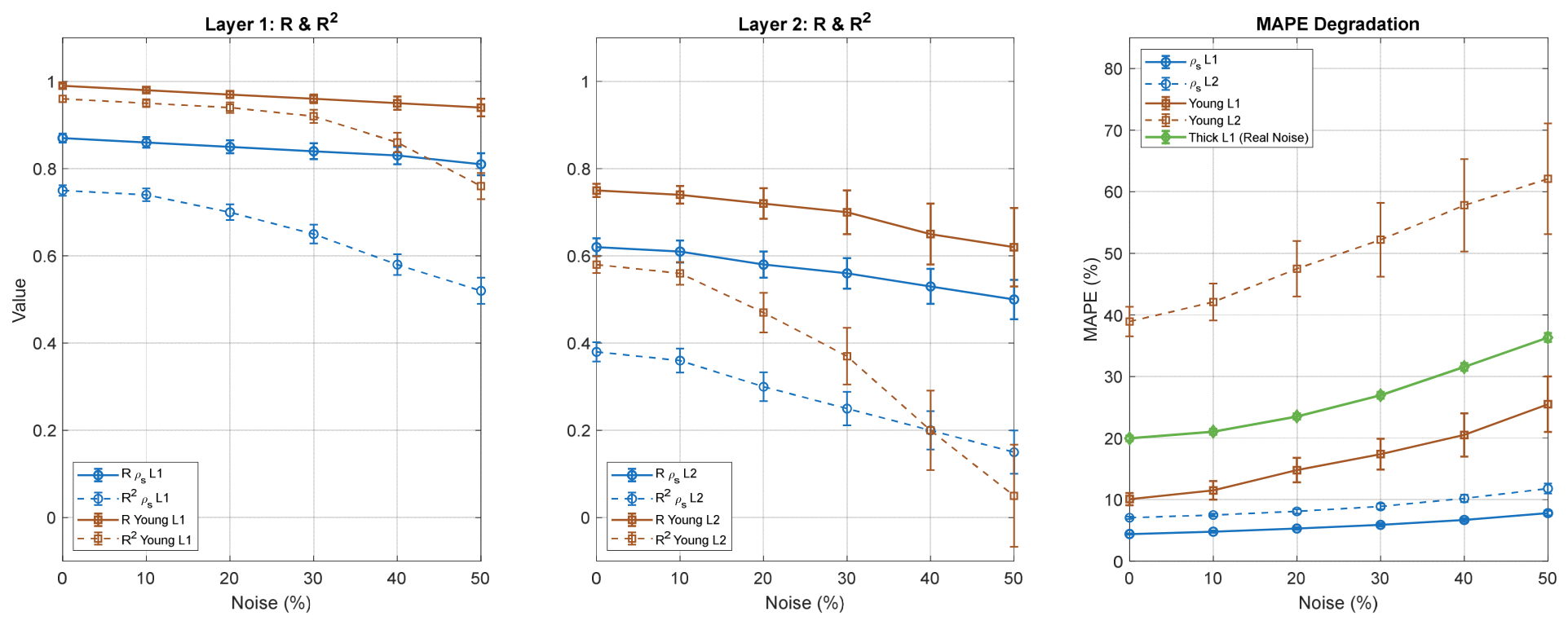
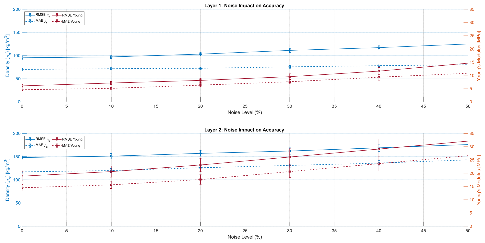
Figure 11, Figure 12 and Figure 13 collectively evaluate the robustness of the CNN models by illustrating the evolution of key performance metrics—correlation (R), coefficient of determination (R²), and various error measures—as increasing levels of Gaussian noise (from 0% to 50%) are introduced into the input seismic data. Specifically, Figure 11 focuses on how noise impacts the model’s linear relationship, explained variance, and percentage error across both layers.

Figure 11 demonstrates the architecture’s robustness evolution against varying levels of synthetic noise, testing its predictive limits up to a severe 50% interference threshold. The models demonstrate significant resilience, particularly for L₁, where the R and R² experience only a gradual and controlled decline despite significant signal degradation. Correspondingly, the MAPE for L₁ density exhibits exceptional stability, remaining tightly constrained below 10%, while Young’s modulus and raw-signal thickness errors scale linearly and maintain practical bounds even under maximum noise exposure. As anticipated by the physical principles of wave propagation, the deeper L₂ exhibits a more pronounced sensitivity to noise due to the inherently lower signal-to-noise ratio of the attenuated subsurface reflections.

Figure 12 delves into the model’s absolute and normalized error performance for density (ρ_s) and Young’s modulus as noise levels progressively increase from 0% to 50%.

Figure 12 expands on the noise sensitivity analysis by detailing the progression of absolute (RMSE and MAE) error metrics under increasing synthetic interference. For L1, the error magnitudes exhibit a controlled and gradual degradation. This indicates the network’s capacity to extract resilient features from contaminated surface-level reflections. As physically expected, L2 displays higher baseline errors and a steeper performance decay. This variance mirrors the compounded effects of wavefield attenuation and the inherently lower signal-to-noise ratio of secondary reflections, confirming that the model behaves in accordance with geophysical principles. Overall, these error dynamics show that the proposed methodology maintains practical parameter estimation under severe operational noise conditions.

To successfully bridge the “sim-to-real” gap and transition this framework to physical field campaigns, several real-world geomechanical factors must be systematically addressed. While this proof-of-concept relies on controlled 2D FEM simulations with idealized transient point loads, actual field environments introduce factors like spatial soil heterogeneity, uncertain absorbing boundary conditions, and source signature variations. In this study, high Gaussian noise thresholds (up to 50%) were actively integrated to serve as a numerical buffer against environmental and sensor-induced interference. For practical site deployment, a Transfer Learning (TL) strategy will be adopted: the network weights optimized on the comprehensive synthetic dataset will serve as a baseline, requiring only a limited set of experimental field measurements, such as borehole logs or Multichannel Analysis of Surface Wave (MASW) profiles, to perform fine-tuning. This localized calibration will adapt the deep learning model to specific 3D wave dissipation patterns and site-specific geological anomalies without requiring computationally prohibitive field training sets.

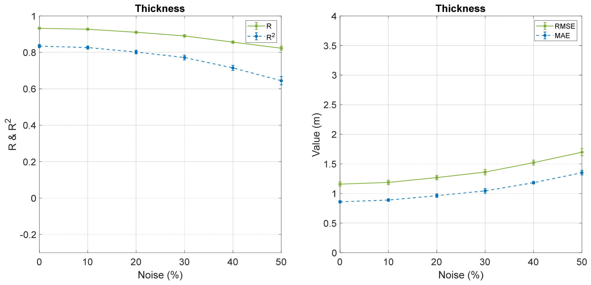
Figure 13 provides a focused analysis of the CNN model’s performance regarding Layer 1 thickness as noise levels scale from 0% to 50%.

Figure 13 shows the impact of synthetic noise on the first layer’s thickness (h₁ estimation derived from the raw-signal approach). The performance metrics display a gradual degradation as interference increases up to the 50% threshold. The R² decreases from approximately 0.83 at baseline to 0.64, while the absolute error metrics exhibit a proportional linear increase, with the MAE rising from 0.86 m to 1.35 m. The low variance across the cross-validation folds confirms stable model behavior under varying signal-to-noise ratios. These dynamics indicate that direct time-domain processing retains practical spatial resolution and predictive reliability even in highly contaminated operational environments.

4.5. Computational Efficiency Cost—Comparison with Full Waveform Inversion (FWI) Methodology

As demonstrated in recent studies regarding the application of machine learning in geotechnics [43], the practical viability of an inversion method depends not only on its accuracy but fundamentally on its computational cost and scalability.

This section compares the computational performance of the CNN model approach against a classical Full Waveform Inversion (FWI) method based on iterative optimization. The analysis is divided into two distinct phases, the Offline Phase (training/preparation) and the Online Phase (Real-time Inference).

To establish a baseline comparison, the conventional FWI routine was implemented via the bounded nonlinear least-squares optimization solver (lsqnonlin) in MATLAB, focusing on minimizing the raw residuals between the forward-modeled structural seismograms and the target surface array observations. To ensure consistency in the physical modeling, the same finite element forward modeling framework used for data generation was employed in the FWI forward simulations. The convergence criteria for this iterative inverse solver were defined with a maximum of 100 iterations, a function tolerance of 1 × 10⁻⁶, and a step tolerance of 1 × 10⁻⁶. To ensure a comprehensive search domain that encompasses the entire parameterized space with an operational margin, the numerical search bounds were specified in geomechanical units: bulk weight density ranged between 10 and 30 kN/m³ (encompassing the simulated 1350 to 2040 kg/m³ mass density range), Young’s modulus between 10 and 500 MPa, and the top layer thickness between 0.5 and 15.0 m. Computational execution times for both the FWI iterations and the neural network inferences were measured on the same computational hardware platform used throughout all experiments, utilizing a Dell Precision Tower 7910 workstation powered by an Intel Xeon E5-2699 v4 processor (2.20 GHz) equipped with 128 GB of RAM and an NVIDIA Quadro M2000 (4 GB) graphics card. While this benchmark ensures consistent and comparable computational conditions across methods, it is acknowledged that FWI performance remains highly sensitive to implementation details and convergence criteria, meaning the reported runtime should be interpreted as representative of this specific numerical setup rather than a general performance bound.

The hardware setup used in this research consisted of a Dell Precision Tower 7910 workstation powered by an Intel Xeon E5-2699 v4 processor (2.20 GHz), equipped with 128 GB of RAM and an NVIDIA Quadro M2000 (4 GB) graphics card.

Table 3. Comparison of computational costs: classical FWI vs. CNN model.

Process Phase	Classical FWI (Iterative)	CNN Model	Remarks
Model Training	N/A (0 h)	≈213 h	FWI has zero setup cost; CNN requires a significant upfront investment.
Inference Time (Single Case)	≈180 s (3 min)	0.035 s	The CNN model is approximately 5000 times faster.
Total Effort (5000 cases)	≈250 h	≈213 h + 3 min (Inference of 5000 cases)	Even including the training time, the CNN model is faster overall.
Marginal Cost	High (Linear)	Negligible	Cost for new cases is virtually zero, for the CNN model.

summarizes the total computational effort required for this study (involving a dataset of 5000 soil profiles). The CNN training time corresponds to a rigorous nested cross-validation process (5 Folds) combined with Bayesian Hyperparameter Optimization, totaling approximately 213 h of computation.

Table 3 compares the computational efficiency of the classical Full Waveform Inversion (FWI) approach and the proposed CNN model. While FWI requires zero upfront training, its inference cost of approximately 180 s per simulation accumulates linearly, totaling around 250 h to process the 5000 cases in this study. In contrast, the CNN demands a substantial initial training investment of 213 h. However, with an inference time of just 0.035 s per simulation, the trained model processes the entire dataset in under 3 min. This negligible marginal cost renders the deep learning approach overall more efficient for the scope of this project, demonstrating its practical superiority for processing large-scale datasets or continuous real-time monitoring scenarios.

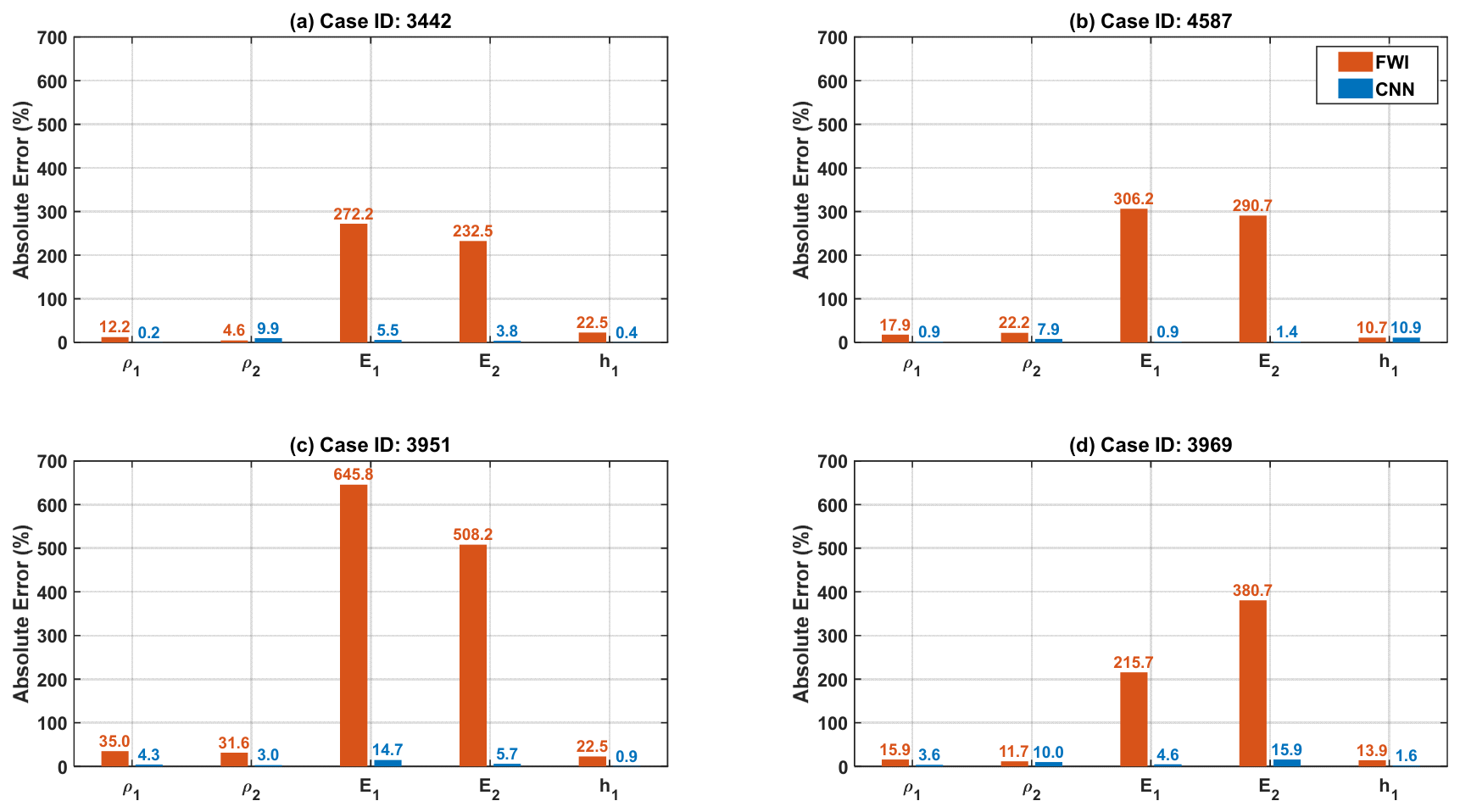
To complement the global assessment and elucidate the sources of the observed performance discrepancies, Figure 14 presents a detailed breakdown of the absolute error across physical parameters (ρ₁, ρ₂, E₁, E₂, h₁) for four selected representative cases.

Figure 14 illustrates a performance disparity between the classical FWI method and the proposed CNN model. The FWI approach yields high global errors, driven primarily by a specific vulnerability in estimating elastic moduli (E₁, E₂), where it frequently converges to local minima. FWI estimates densities (ρ₁, ρ₂) and the first layer’s thickness (h₁) with errors generally below 35%. While these deviations are typically higher than the CNN’s baseline, case 4587 presents a singular exception where FWI marginally outperforms the CNN in determining h₁ (10.7% versus 10.9%). Despite this isolated instance, the overall results confirm that the deep learning architecture captures the complex nonlinear relationships between waveforms and soil properties, decoupling the influences of stiffness, density, and geometry without the convergence limitations inherent to classical iterative methods.

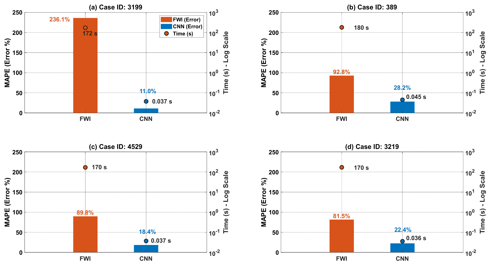
Figure 15 synthesizes the global efficiency and accuracy of both methods into a single dual-axis chart. The vertical bars (referenced to the left linear axis) depict the average error (MAPE), while the two discrete markers (referenced to the right logarithmic axis) indicate the computational time required per inversion.

The results show a clear divergence in performance. The FWI method requires approximately 180 s per case and results in higher error rates for these scenarios. In contrast, the CNN model reduces the processing time to 0.035 s while maintaining low error levels. This confirms that the computational speed of the neural network does not negatively impact its accuracy. The CNN proved to be both faster and more precise than the iterative approach.

4.6. Overall Considerations and Future Perspectives

The FEM simulation framework enabled the generation of a comprehensive dataset across a wide parametric space, facilitating training of the predictive models.

The use of a 2D finite element formulation introduces a dimensionality reduction in the full 3D elastic-wave propagation problem. In 3D media, wavefields generated by point sources exhibit spherical geometric spreading, whereas 2D simulations correspond to cylindrical line-source propagation. This leads to a fundamental difference in amplitude scaling and energy distribution between the two formulations.

Established elastodynamic theory and numerical benchmarks [44,45,46] show that the impact of this dimensionality reduction is strongly dependent on the type of observable considered. Kinematic features, including first-arrival travel times and phase structure, are primarily governed by the elastic velocity field and are comparatively robust to dimensionality reduction in layered isotropic media. In contrast, amplitude- and attenuation-related observables are highly sensitive to dimensionality due to geometric spreading effects and the absence of out-of-plane wave propagation in 2D simulations.

As a result, no single universal quantitative error bound exists for 2D–3D differences, as these depend on source–receiver geometry, frequency content, and heterogeneity complexity. Instead, the established classification in the literature distinguishes between kinematically stable observables and dynamically sensitive amplitude-related quantities.

Since the proposed learning framework is driven primarily by kinematic waveform features rather than absolute amplitudes, the 2D-generated dataset remains physically consistent for the intended inverse problem. A full 3D numerical benchmark is identified as future work for quantitative calibration of amplitude-related effects. To evaluate the generalization limits and robustness of the convolutional framework, the synthetic seismograms were subjected to severe Additive White Gaussian Noise (AWGN) levels, with standard deviations scaling up to 50%. It is important to emphasize that this represents a considerable simplification of physical ambient noise fields, which are inherently colored, non-stationary, and dominated by structured microseisms or cultural site noise. The utilization of AWGN serves as a conservative, worst-case numerical benchmark because white noise distributes its stochastic energy uniformly across the entire frequency spectrum and it directly contaminates the critical passband of the seismic source wavelet, imposing a harsher feature-extraction penalty than sparse out-of-band noise. In field deployment scenarios, this simplification might theoretically overestimate robustness if highly coherent, in-band non-stationary noise is present. However, in routine engineering seismology practice, this vulnerability is heavily mitigated during data preprocessing. Raw field records are standardly processed using zero-phase band-pass filters and trace normalizations designed to isolate the active source spectrum and attenuate out-of-band colored environmental components. The residual noise level is typically reduced in amplitude and bandwidth after preprocessing, partially mitigating the discrepancy between AWGN and field noise. Nonetheless, this study does not explicitly model colored or non-stationary noise processes, which may exhibit different coherence structures in field conditions. Incorporating such noise models remains an important extension for future work.

The models’ resilience to typical signal corruption suggests that the transition to experimental prospecting is computationally and physically feasible. Beyond these data corruption filters, an additional consideration concerns the model’s extrapolation capability outside the calibrated geomechanical ranges defined in Table 1. As a regression-based deep learning framework, the network is primarily trained to perform accurate interpolation within the bounded parameter space represented in the synthetic dataset. When applied to conditions outside this range, a degradation in predictive performance may occur due to distributional shift between training and unseen geomechanical scenarios. This limitation is inherent to supervised learning approaches trained on finite datasets and should be considered when deploying the model in new geological settings. In such cases, transfer learning may provide a practical adaptation strategy, where pre-trained convolutional feature extractors are retained and the final regression layers are fine-tuned using a limited amount of site-specific data. Structurally, a critical finding remains the decisive improvement in computational efficiency achieved by the framework. Although the initial investment requires approximately 63 h for database generation and 213 h for training (with our hardware and software setup), the resulting online inference phase performs a full parameter estimation in 0.035 s. This speed increase of over three orders of magnitude compared to classical FWI enables real-time monitoring and large-scale parametric studies that were previously computationally prohibitive. Future research will integrate Explainable AI (XAI) techniques, such as SHAP, to verify that the predictive logic aligns with physically sound wave propagation principles and focus on validating these models with experimental field data.

5. Conclusions

This research introduces a physics-based deep learning framework that transforms FEM-generated displacement signals into comprehensive property estimations for layered media. The results demonstrate that while a CNN effectively extracts density and stiffness parameters from composite time–frequency images, a direct time-domain raw-signal approach is required to accurately resolve the first layer’s thickness (h₁). The models achieve high accuracy for near-surface characterization, with Layer 1 Young’s modulus reaching a coefficient of determination (R²) of 0.96 and the raw-signal thickness estimation achieving an R² of 0.83.

A distinct performance gradient was observed across the physical strata, highlighting a fundamental physical boundary for surface-based seismic prospecting. While shallow parameters were predicted with high stability and precision, the predictive reliability visibly decays within the deeper stratum, where the R² values for Layer 2 properties drop below 0.60. This degradation is physically consistent with the natural geometric dispersion and scattering of secondary reflections at depth, which drastically diminishes the signal-to-noise ratio of waves returning from deeper layer interfaces. Consequently, while the framework establishes an exceptionally reliable baseline for near-surface characterization, its predictive capacity for deeper formations remains bound to these physical attenuation constraints, and interpretation at depth should be approached with appropriate engineering margins.

The reliability of these conclusions is supported by an exhaustive statistical validation scheme, including nested 5-fold cross-validation, normality assessments, and 95% bootstrap confidence intervals. Furthermore, the framework demonstrated robustness to synthetic Gaussian noise. Although performance for deeper features predictably declined under extreme interference, the direct time-domain approach for estimating h₁ maintained practical reliability, with its R² sustaining a value of 0.64 even at 50% noise. A comparative analysis with classical Full Waveform Inversion (FWI) revealed a decisive operational advantage: the machine learning pipeline reduced inference time from 180 s to 0.035 s while avoiding the local minima convergence issues inherent to iterative methods. By establishing the computational feasibility of using processed and raw seismograms for rapid characterization, future efforts will focus on bridging the sim-to-real gap through experimental field validation and integrating Explainable AI techniques to enhance model transparency.