Article

Pre-Event Estimation of County-Level Human Casualty Projections in Southwestern China Based on the Spatial Aggregation of Village-Scale Lethality Data

1
Key Laboratory of Seismic and Volcanic Hazards, China Earthquake Administration, Beijing 100029, China
2
Institute of Geology, China Earthquake Administration, Beijing 100029, China
3
Ningxia Seismological Bureau, Yinchuan 750001, China
4
Xinjiang Pamir Intracontinental Subduction National Observation and Research Station, Beijing 100029, China
5
China Earthquake Networks Center, Beijing 100029, China
*
Author to whom correspondence should be addressed.
Deceased author.
Appl. Sci. 2026, 16(12), 6257; https://doi.org/10.3390/app16126257
Submission received: 9 February 2026 / Revised: 11 April 2026 / Accepted: 14 April 2026 / Published: 22 June 2026

Abstract

An earthquake lethality model was employed to assess the casualty distribution in Yunnan, Guizhou, and Sichuan provinces, taking into account the ground motion acceleration with different 50-year exceedance probabilities. When the probability is 63%, fatalities are predominantly concentrated in central and south-western Yunnan, as well as central, southern, and western Sichuan. At a 10% probability, the peaks of the casualties are observed in southern, eastern, and central Sichuan. In Yunnan (excluding the northwest and southeast regions), the casualty density exhibits unevenness, whereas Guizhou experiences relatively low casualties (except in the eastern and western mountainous areas). Xichang incurs the most substantial losses, followed by Lancang. Xundian, Songming, and Dongchuan demonstrate a high propensity for fatalities, and the risk is relatively high in the vicinity of the Longjiang and Nujiang faults. If a destructive earthquake occurs near these areas within the next 50 years, the probability of a Level-I emergency response exceeds 10%. When the ground motion acceleration doubles (especially when the exceedance probability drops to 2% in 50 year and 0.1% in a year), the predicted number of casualties remains relatively stable. However, the grid of the casualty population exhibits a higher degree of spatial concentration of casualties, and the disaster-affected area expands. There exists no linear correlation between earthquake-induced fatalities and the ground motion level. When the 50-year exceedance probability decreases from 63% to 10%, the casualty rate may increase by several dozen times.

1. Introduction

The primary objective of pre-assessment is to identify counties with a high expected risk of casualties for emergency management departments, designating them as key areas of concern. This enables the coordination of resources to conduct risk management and emergency preparedness in a scientific and effective manner. The assessment encompasses various methods, including model-based evaluation, field surveys, expert assessments, and subsequent revisions.
Traditionally, pre-earthquake casualty assessments have focused on three main elements: earthquake risk, building vulnerability, and resident exposure. For instance, a vast region stretching from Sichuan’s Daofu to Yunnan’s Qiaojia, encompassing parts of Yunnan, Guizhou, and Sichuan, has been designated as a key risk area by the China Earthquake Administration (CEA). The 2008 Wenchuan earthquake resulted in $124 billion in indirect losses, which accounted for 40% of the direct losses, with the casualty count exceeding 80,000 [1]. Regarding vulnerability, building collapse/damage and secondary disasters are the primary contributors to casualties [2]. There exists a correlation between the number of casualties and the number of collapsed/damaged buildings [3,4]. The vulnerability level of buildings is primarily associated with the probability of different damage states under various earthquake magnitudes or intensity ranges [5], which is not directly related to the death of individuals. The so called lethal level refers to the comprehensive likelihood or level of multiple factors that lead to death due to building destruction, expressed in terms of the higher mortality rate at each intensity level [6]. Building on this, it is mainly associated with the disparity in buildings’ ability to cause casualties. In essence, the lethal level considers the probability of death under various intensities, factoring in the overall quantitative level of multiple factors in the affected area. It also accounts for situations such as “destruction without collapse, collapse without death,” meaning the potential for survivors in the reserve space [6]. The last factor is population exposure. With the steady advancement of urbanization in China, large and medium-sized cities have significantly increased their population concentration, making them more susceptible to the impact of earthquake risks. Enhancing the accuracy and efficiency of casualty assessments can provide valuable insights for decision-makers, insurers, real estate brokers, and other stakeholders. This helps them to adjust economic development models, enhance building resilience, scientifically refine disaster insurance strategies, and improve the operability of disaster insurance. The ultimate goal is to ensure the safety of people’s lives and property and to secure the long-term stable development of society.
The previous risk assessment was constructed based on a comprehensive analysis of historical earthquake data, vulnerability of buildings and secondary geological disasters, and the evaluation methods can be categorized into two groups. The first category is the empirical function method, which is based on seismic parameters and population density [7,8,9,10,11,12]. Among these [13], proposed a neural network model of seismic activity that considers factors such as intensity, seismic depth, fortification level, population density, etc. Ref. [14] used a vulnerability curve to express the relationship between seismic intensity and mortality across China and Western China. Certain researchers have proposed a probability model utilizing modified empirical mortality data [15,16], whereas other scholars have developed the Asian Earthquake Death Rapid Assessment Model (QAMECA), which incorporates earthquake intensity and additional factors [17]. However, the above method only utilizes the seismic parameters of historical earthquakes, rendering the model ineffective in areas lacking earthquake data and leading to inaccurate results. The second category is based on the vulnerability and lethality of buildings, constructing a model through the statistical fitting relationship between the vulnerability, lethality, and casualties of buildings, and using the regression of vulnerability function to assess casualties [18,19,20]. The vulnerability of buildings refers to their ability to withstand and recover from the impact of hazardous events [21]. These methods fully consider the impact of building damage on the number of deaths, thereby improving calculation accuracy. For example, certain scholars have identified principal determinants influencing casualty levels during seismic events, including building characteristics, occupancy rates, and timing of occurrence [22]. Other researchers have developed vulnerability functions for various structural types, which quantify the relationships among construction materials, extent of damage, and resulting fatalities [23]. Additionally, studies have employed GIS-based building damage datasets to support modeling and casualty estimation [4,24]. Based on the vulnerability of various buildings in Greece [25], estimated casualties by considering the collapse probability of buildings under the influence of factors such as intensity and occupancy rate. A study proposed the scale of the relationship between building damage and casualties, along with a corresponding casualty assessment methodology [26]. Research has introduced a classification system for building damage, categorizing it into total collapse and total destruction, and established a correlation between damage grade and mortality rate [27]. Scholars have developed a casualty estimation model based on a building vulnerability matrix [28]. Furthermore, some authors have constructed relationships between casualty distribution and explanatory variables, such as building type and degree of damage, leading to the development of a prototype global casualty assessment model [29]. Due to the lack of data accuracy, model inapplicability, and quantitative lethal effect assessment of casualty factors (such as building damage, secondary geological disasters, major hazard sources, falling objects, crowd congestion, non-structural partial damage, adverse evacuation caused by traffic damage, etc.), the accuracy and regional applicability of these assessments are, to varying degrees, insufficient to meet actual needs.
The survival rate of individuals trapped during earthquakes is typically nonlinear and inversely proportional to the duration of the pressure they endure. In response to the need for rapid and accurate assessment, new demands have emerged for seismic pre-assessment and risk assessment, including the distribution of earthquake-buried personnel, necessitating the exploration of new models and data. Since China’s accession to the WTO (World Trade Organization), the urbanization process has accelerated, and research on urban disaster assessment and management requires enhancement. Chinese scholars have conducted assessments of casualties or economic losses based on building vulnerability. Researchers have estimated the proportion of rural houses across diverse structural groups in China through a downscaling methodology that incorporates nonlinear regression, probabilistic risk prediction, and a cumulative probability model, thereby evaluating the vulnerability at the county level [30]. A separate study established an empirical vulnerability matrix for typical building groups within varying seismic intensity zones in Dujiangyan City [31]. By employing data mining and geoscience techniques, specifically support vector machines and association rule learning, investigators applied the seismic vulnerability index to Urumqi and verified its effectiveness [32]. Additionally, another research effort utilized the beta probability density function to derive the earthquake vulnerability matrix for rural areas in Weinan, revealing the distributions of the earthquake damage index and damage rate [33]. These previous assessment methods based on building lethality have limitations: (1) most existing methods rely on the vulnerability level of buildings, neglecting the diversity of building lethality and the influence of other factors. Historical earthquake analyses indicate that different regions may exhibit similar fractional intensity lethal levels under the combined effects of buildings, geographical environment, secondary disasters, and accidental factors, while the probability of death from buildings with similar vulnerability levels can vary significantly across different events [5,34,35]. In reality, a high building damage rate does not always correspond to a high mortality rate [36]. (2) In model construction and evaluation, if the analysis is based solely on the overall mortality rate in the affected areas rather than specific zones, its accuracy may be compromised, and it is challenging to capture the specific mortality characteristics of areas with varying residential densities and building structure types.
Thus, determining the lethality of a specific area is crucial. Addressing these shortcomings, someone conducted an effect analysis of lethal factors in various regions, constructed the lethal matrix for different factors in those regions, and established medium and long-term risk assessments, pre-earthquake assessments, and post-earthquake rapid assessments using quantitative methods [37]. Based on historical casualties, a rapid assessment matrix for casualties was constructed according to the anti-fatality level and the mortality rate of each intensity level [6,38,39,40]. The method is semi-empirical, and its origin has been explicitly delineated: the lethality theory, which is founded on historical earthquake data, represents a contribution introduced by the authors of reference [37], and it was initially developed as an extension of the model proposed by the aforementioned authors [41]. This study has conducted large-scale lethality analysis and casualty assessment in China, and valuable results have been obtained [37,38,39].
The existing empirical function approach constructs models by leveraging historical seismic data and seismic parameters (e.g., magnitude, earthquake depth, population density, etc.). However, its performance is less than ideal in regions with a dearth of seismic data, frequently resulting in inaccurate outcomes. Although the current regression analysis method of vulnerability functions enhances accuracy by establishing statistical fitting relationships among building vulnerability, lethality, and casualty numbers, fully taking into account the impact of building damage on fatalities, such methods are constrained by data accuracy, model applicability, and the quantitative assessment of lethal effects from multiple casualty-inducing factors (e.g., secondary geological hazards, major hazard sources, crowd congestion, non-structural damage, and evacuation difficulties caused by traffic damage). More crucially, most existing methods for assessing building lethality solely rely on building vulnerability levels, overlooking the diversity of building lethality and the influence of other factors. Moreover, existing models that only analyze the overall mortality rates in affected regions rather than in specific sub-regions lack in-depth studies on earthquake damage and casualty assessments at the community/village level for specific seismic risk areas. Their accuracy may be impaired, and they find it difficult to accurately reflect the unique mortality patterns in regions with varying residential densities and building structure types. In China’s seismic risk areas, research on evaluating earthquake disaster casualties under different seismic activity probability levels is also relatively limited.
In summary, the limitations of extant methods encompass the following:
(1)
Integrating household proportions across diverse building structures and fatality resistance levels to determine the regional overall fatality resistance threshold;
(2)
Converting seismic intensity vector data into grid format while preserving essential characteristics, pruning population grid data to align with regional boundaries, and ensuring coordinate system consistency;
(3)
Calculating matrices by overlaying seismic intensity, population distribution, and fatality levels, performing conditional grid allocation operations, and combining spatial analysis to aggregate casualty estimates for administrative regions, thereby achieving refined multi-source data integration and grid-level estimation.
In contrast, the method proposed in this study marks the initial endeavor to leverage data from the Seventh National Population Census [42,43,44,45] conducted by the National Bureau of Statistics for evaluating building-related casualties at the county level, enabling more refined casualty assessments at the district and county levels. The core methodology entails calculating the lethality levels of diverse building structures to obtain the overall lethality metrics for earthquake-prone regions. Lethality is, in essence, a parameter calibrated by means of historical mortality data. The lethality scale consists of 11 levels spanning from 0 to 1, which can be directly interpreted via casualty ratios with an error margin of ±50%. This suggests that lethality levels represent quantified parameters obtained from historical mortality data through calibration procedures. By integrating data on the resistance of building structures to lethality, population distribution patterns, and other relevant factors, we ascertain the casualty ratios for specific regions under given seismic intensity levels using the lethality/resistance matrix. The entire methodology hinges on a comprehensive analysis and calibration of historical mortality data. Although geographical conditions, secondary disasters, and accidental factors may impact the outcomes, this approach explicitly designates structural composition and lethality as the primary determinants. By collecting regional lethality data during surveys, post-earthquake casualty assessments can be carried out based on the regional lethality capacity and the population corresponding to intensity levels.
This method not only inherits the theoretical basis of the semi-empirical casualty rapid assessment matrix developed from the historical earthquake lethality theory [37], but also fills the methodological gaps in assessing casualties in community/village-level seismic risk areas and under varying earthquake activity probabilities; specifically, by integrating national census data, detailed seismic intensity zoning, and demographic distribution patterns with lethality matrix-based data processing techniques and evaluation models, it precisely reflects the casualty patterns across regions (e.g., Yunnan, Guizhou, and Sichuan provinces) within the updated intensity zoning frameworks, taking into account local housing structures and population distribution characteristics, achieves substantial improvements in assessment precision at the district and county levels, surmounting the previous model limitations in regional applicability and localized fine-scale evaluation, and addresses the research gaps encompassing substantial inaccuracies in lethal dose level assessment (±50%) and the absence of methodologies for converting county-level household statistical data into kilometer-scale fine-grained data. This model incorporates capabilities for data spatialization and refinement, emphasizing the spatialization of demographic and socio-economic variables along with precise, quantitative, and cyclically updated mortality metrics to enhance data accuracy, which distinguishes it from coarse-scale applications such as the HAZUS (Hazardous US, developed and maintained by the U.S. Federal Emergency Management Agency, is a standardized multi-hazard risk assessment methodology widely employed in seismological research for conducting detailed risk analyses and loss estimations associated with seismic events. This framework enables the quantitative evaluation of earthquake impacts, encompassing casualties, structural damage, economic losses, and infrastructure disruption. It thereby serves as an essential tool for informing disaster risk management strategies and enhancing emergency preparedness.) framework; it develops region-specific lethality matrices—including regional mortality and injury matrices—tailored to different geographical contexts, thereby overcoming the limitations of generalized empirical casualty functions; structured to evolve into a comprehensive multi-factor integration framework, it is capable of incorporating “secondary disaster-chain matrices,” “soft impacts derived from public sentiment,” “indirect economic losses,” and full-scale disaster-bearing structure data (e.g., proportions of brick-wood and earth-wood building types) to achieve end-to-end simulation, extending beyond HAZUS’s primary focus on direct casualties from single-event disasters; with dynamic spatiotemporal integration capabilities, it supports multi-temporal risk assessments based on “spatiotemporal population distribution,” advancing beyond static empirical functions to enable dynamic evaluation; and is designed to progress toward real-time social-sensing data fusion, allowing for the simulation of earthquake motion parameters (e.g., PGA, PGV) using rapid reporting data and real-time social sensing information to improve temporal relevance, a feature seldom integrated in frameworks such as HAZUS.
This research aims to examine the spatial distribution of earthquake-induced casualties within the Yunnan–Guizhou–Sichuan region. It will evaluate casualty patterns under diverse seismic probabilities and emergency response triggers. Furthermore, it will investigate the nonlinear relationship between ground motion intensity, (exemplified by Peak Ground Acceleration (PGA), and casualty rates, alongside the impacts of building structural characteristics. The research also seeks to enhance rapid assessment methodologies through the development of casualty matrices, analysis of secondary disasters, refinement of models, parameter simulation, dataset improvement, and dynamic mortality mapping for high-risk zones. The spatialization of demographic and socioeconomic data is implemented to enhance assessment accuracy. A nonlinear relationship is posited between casualties and PGA. The integration of remote sensing and machine learning techniques facilitates the generation of refined, quantitative risk layers. This research is anticipated to elucidate casualty distributions and delineate high-risk zones for regional seismic assessment. It will reveal correlations between ground motion parameters and casualties, as well as building impacts, to inform seismic design practices. Additionally, it will improve model accuracy and scalability for pre-disaster risk evaluation and comprehensive disaster simulation.
In this manuscript, we first describe the inputs used, such as national census data, intensity zoning, and population distribution. Next, we introduce our data processing method and evaluation model based on a lethality matrix. Finally, our results include the assessment of casualties in Yunnan, Guizhou, and Sichuan, based on the latest intensity zoning and considering the local housing structure/population distribution, and the assessment of casualties by district/county.

2. Data

2.1. Study Area and Earthquake Distribution

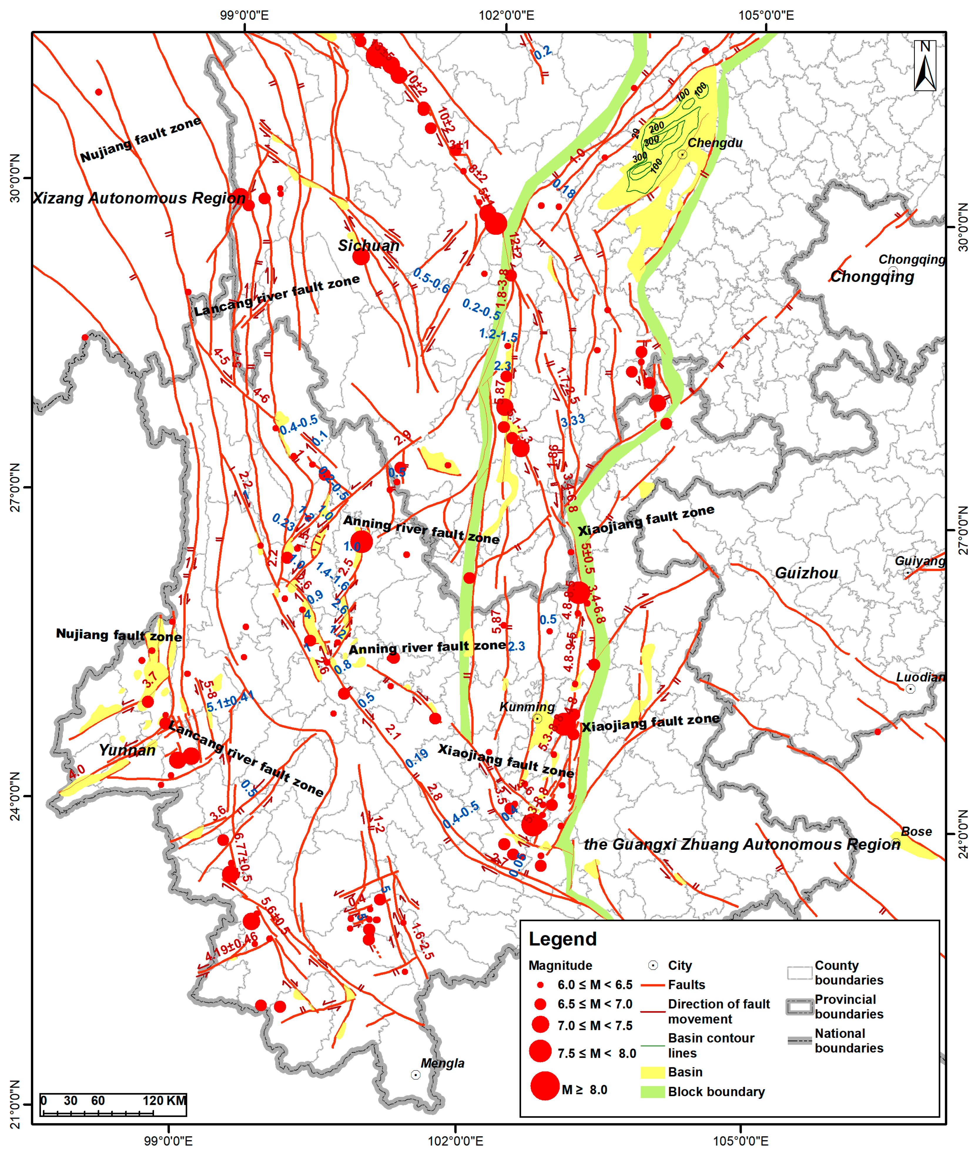
China is one of the countries with the highest number of earthquake casualties in the world. Three of the world’s top ten deadliest earthquakes have occurred in China. As a segment of the Eurasian seismic belt, the North-South Seismic Belt in China is crucial for strong earthquakes occurring in a roughly north-south direction [46,47,48]. Extending from Ningxia to Yunnan, through East Gansu and West Sichuan, and reaching as far as Mongolia in the north and Myanmar in the south, Yunnan, Guizhou, and Sichuan are situated at the southern end of this seismic zone. Nearly half of the earthquakes with a magnitude of 8 and above recorded in China have occurred within this zone, including the 8.0 magnitude Wenchuan earthquake [49,50]. Figure 1 illustrates the distribution of earthquake events with magnitudes of 5.0 and above in Southwest China. The catalog is available at CEDC (China Earthquake Data Center, website: http://data.earthquake.cn). The seismic catalog utilized in this study encompasses the regions of Yunnan, Guizhou, and Sichuan, incorporating both historical earthquake records and instrumentally recorded seismic data. This comprehensive dataset ensures that the temporal duration and spatial extent satisfy the prerequisites for regional seismic risk assessment. Consequently, it provides a robust foundation for constructing mortality/injury matrices, subsequent secondary disaster chain matrices, and dynamic risk assessment models. We consistently employ the M magnitude scale to quantify the magnitude of seismic energy release, making no distinction between Ms (surface wave magnitude, derived from surface wave amplitude) and Mw (moment magnitude, calculated from seismic moment). It is evident that the population density in Yunnan, Guizhou, and Sichuan is relatively high [51] (National bureau of statistics of China, 2025), historically experiencing frequent and destructive earthquakes [52,53,54]. Figure 1 shows the distribution of Richter earthquakes with magnitudes of 5.0 and above. According to the disaster assessment report from 1996 to 2022 [55], the historical earthquakes with magnitudes of 7.0 and above in Yunnan, Guizhou, and Sichuan in China by 2023 are detailed in Table 1.

2.2. Data Sources Used in This Study

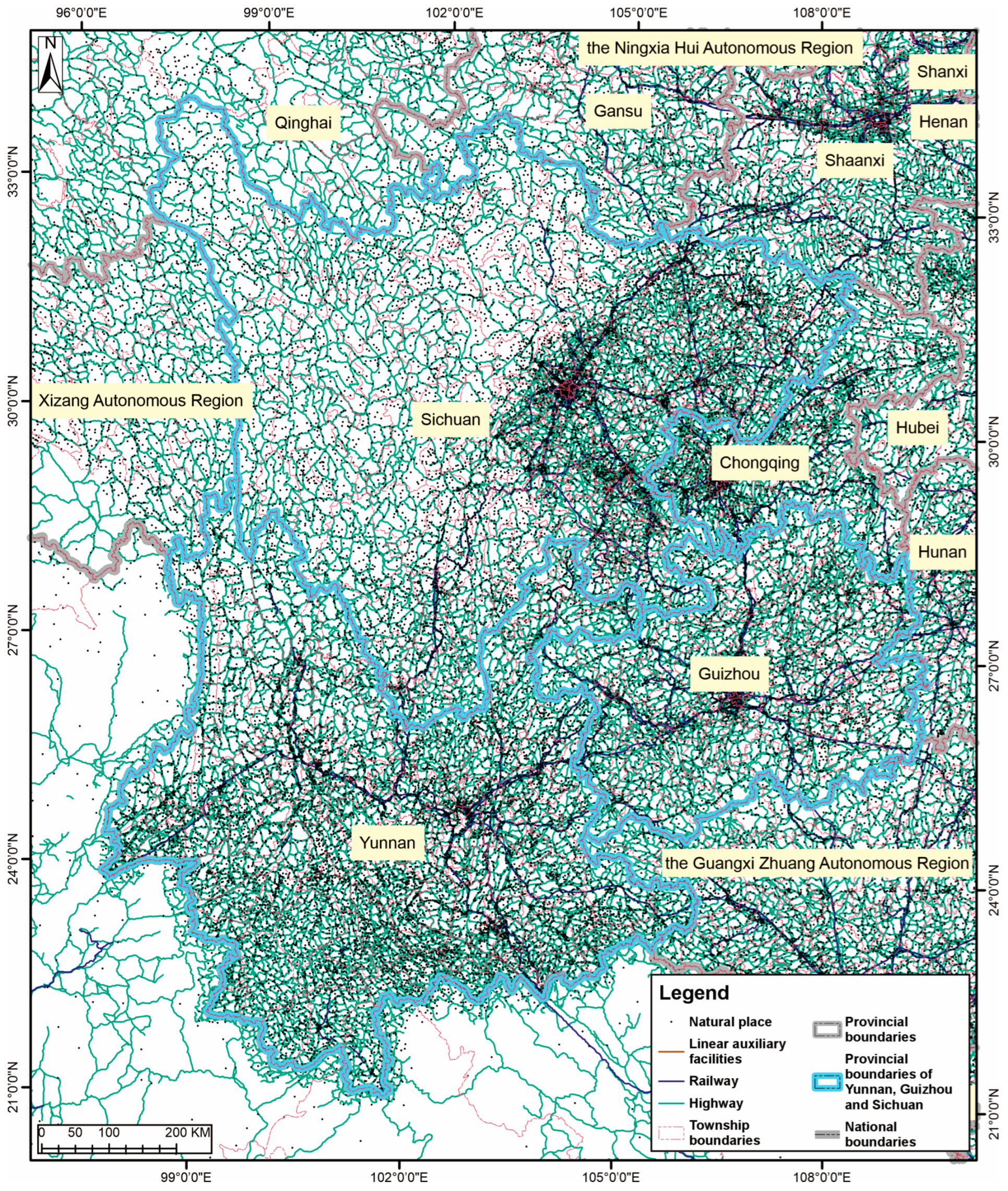
For this study, our foundational geographic information includes the boundaries of administrative divisions. We obtained the national basic geographic data for administrative divisions (version 2019) from the National Geographic Information Directory Service (NGISD), managed by the National Basic Geographic Information Center (NBGIC). We utilized these data, with a scale of 1:250,000, and the division data (version 2021) at a scale of 1:100,000, as our drawing framework (see Figure 2).
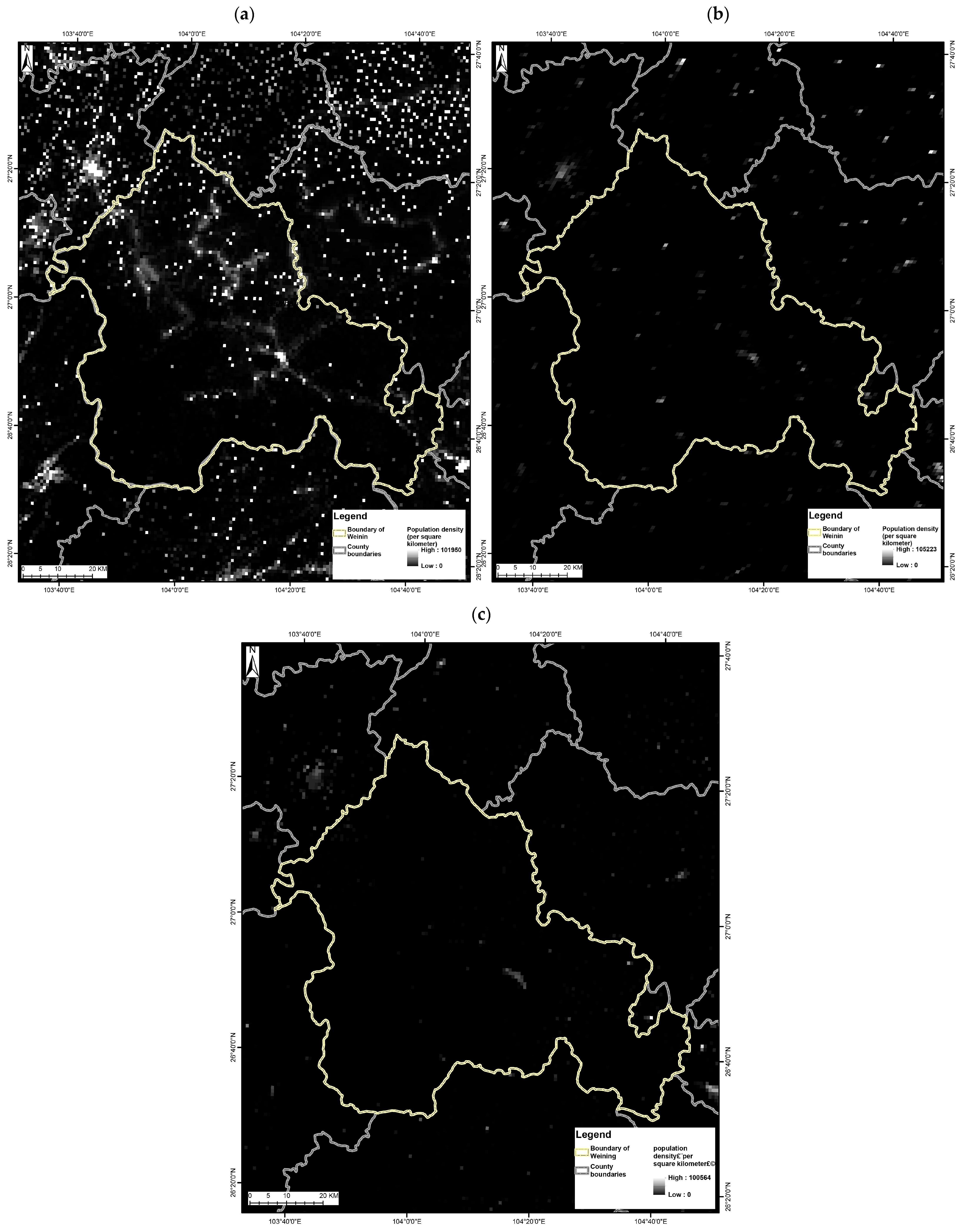
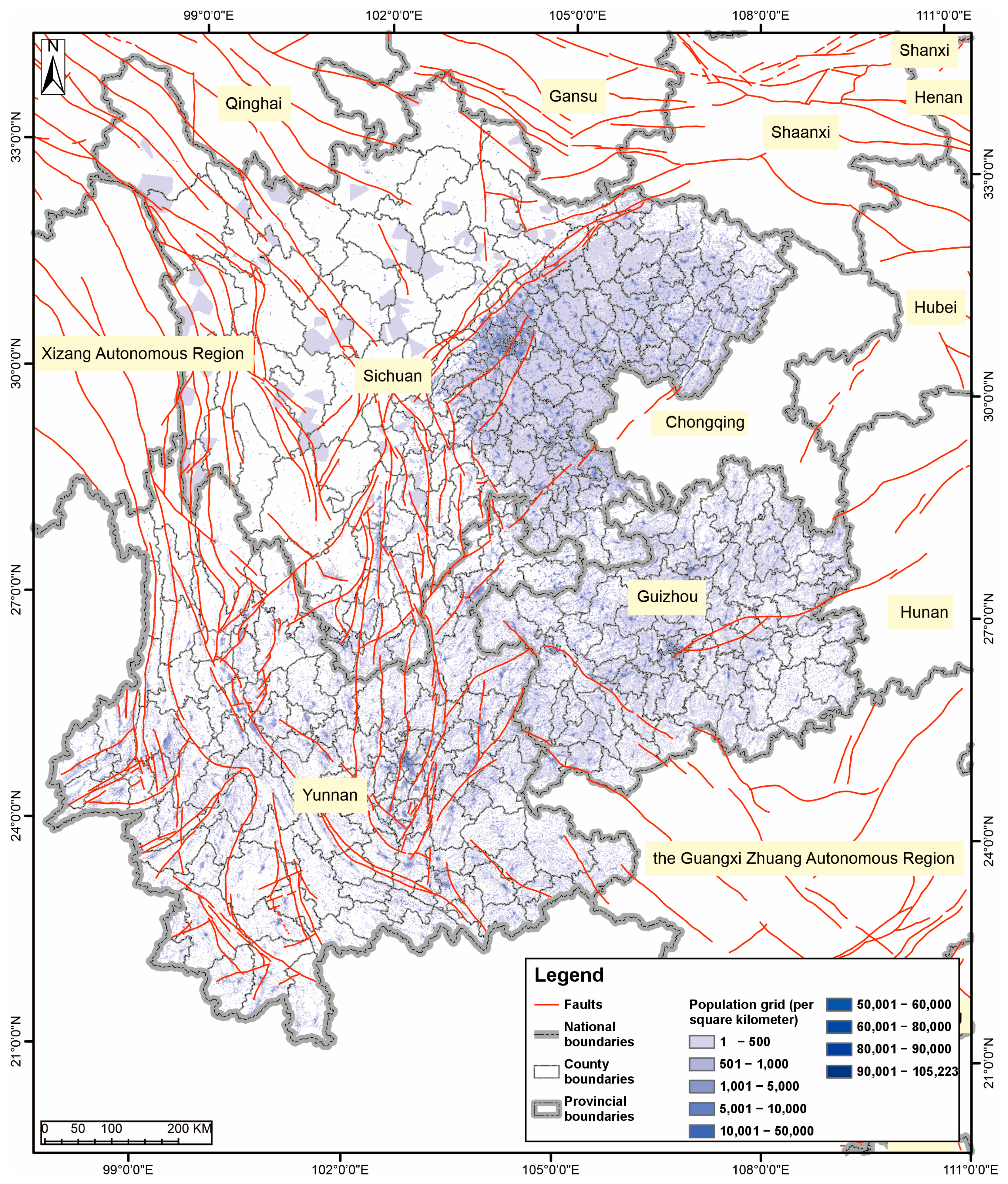
Upon comparison, it was discovered that the population density figures per square kilometer published by the European Space Agency (ESA) and the China Earthquake Administration (CEA) are quite similar. However, the population density data provided by China’s mobile terminal public services appears more varied. When compared with the recently released population data from the local government website as the benchmark, it indicates that the 2020 grid population data (https://ghsl.jrc.ec.europa.eu, accessed on 1 January 2024) published by ESA is more accurate to the actual figures (refer to Figure 3).
To validate the rationale for employing a 1 km × 1 km grid in computational analyses, we augmented the methodology with sensitivity analyses comparing grids of varying resolutions to enhance rigor. Four spatial resolutions (0.5 km, 1 km, 2 km, and 5 km) were evaluated based on multiple criteria: relative errors in total casualty counts across resolutions, alterations in high-density hotspot areas (e.g., regions exceeding 100 fatalities per km2), variations in spatial clustering patterns of casualties (e.g., patch sizes of high-risk zones), and root mean square errors (RMSE) between resolution outcomes and ground truth values (assuming the 0.5 km resolution as the finest reference). Results indicate that the 0.5 km resolution more accurately captures local variations in population and building distributions (e.g., urban neighborhoods and rural villages). By minimizing spatial averaging errors, it facilitates clearer identification of small-scale high-risk hotspots (e.g., densely populated residential areas in Xichang characterized by low seismic reinforcement rates). However, computational costs increase approximately three- to fivefold relative to the 1 km resolution. The 1 km resolution achieves an optimal balance between accuracy and efficiency: while casualty density distribution patterns align closely with those derived from the 0.5 km resolution, minor smoothing effects may occur in small hotspots (<0.5 km2). Relative errors in total casualty counts remain below 5% compared to the 0.5 km resolution. At a 2 km resolution, total casualty counts exhibit an 8–12% relative error relative to the 0.5 km resolution. High-density hotspot areas tend to merge, resulting in reduced spatial resolution (e.g., merging adjacent urban-rural regions in central Sichuan). At a 5 km resolution, total casualties are underestimated by 15–20% in complex terrains such as mountainous areas with scattered villages in western Yunnan. Spatial distribution patterns of casualties become significantly blurred, with high-risk zones overextended by 20–30% (e.g., merging multiple small high-risk grids into large contiguous areas). In urban or high-density regions (e.g., Xichang, Kunming), resolution reduction (from 0.5 km to 5 km) elevates errors (total casualty error range: 15–25%) due to loss of detailed population and building data. Rural or low-density areas (e.g., northwestern Yunnan) demonstrate lower sensitivity to resolution changes: errors remain below 10% at 2–5 km resolutions versus 0.5% at the 0.5 km resolution, as uniform population and building distribution reduces spatial averaging deviations. Sensitivity analysis suggests that optimal resolutions for localized detailed assessments range from 0.5 to 1 km, prioritizing accuracy in high-risk urban or complex areas. Resolutions of 2–5 km are more suitable for regional rapid screening. The 1 km resolution delivers optimal performance across most scenarios with errors below 5%, while the 0.5 km resolution maintains computationally manageable costs.
To validate the rationality of the ESA population grid dataset, we utilized county-level permanent resident population data from the 2020 Seventh National Population Census for Yunnan, Guizhou, and Sichuan provinces as the benchmark (official actual values), encompassing 197 county-level administrative units. Correspondingly, the ESA population grid data (2020 version) at 1 km resolution was aggregated to the county level via spatial overlay analysis in ArcGIS. Consistency and accuracy were assessed using the mean absolute error (MAE), root mean square error (RMSE), correlation coefficient (R2), and the proportion of counties with relative errors within 10%. The results, summarized in the accompanying Table 2, indicate a strong correlation between the ESA population grid estimates and the official census data, with R2 = 0.92. The MAE was 44,000 persons (approximately 5.3% of the average county population), the RMSE was 59,000 persons, and 82.3% of counties exhibited relative errors ≤10%. These error levels fall within the acceptable range for population spatialization studies, where thresholds commonly do not exceed 15%. Furthermore, the 1 km spatial resolution of the ESA grid data allows for a detailed representation of population distribution patterns. In summary, the adoption of ESA population grids is statistically well justified, both in terms of quantitative agreement with census data and the enhanced spatial granularity offered by the dataset.
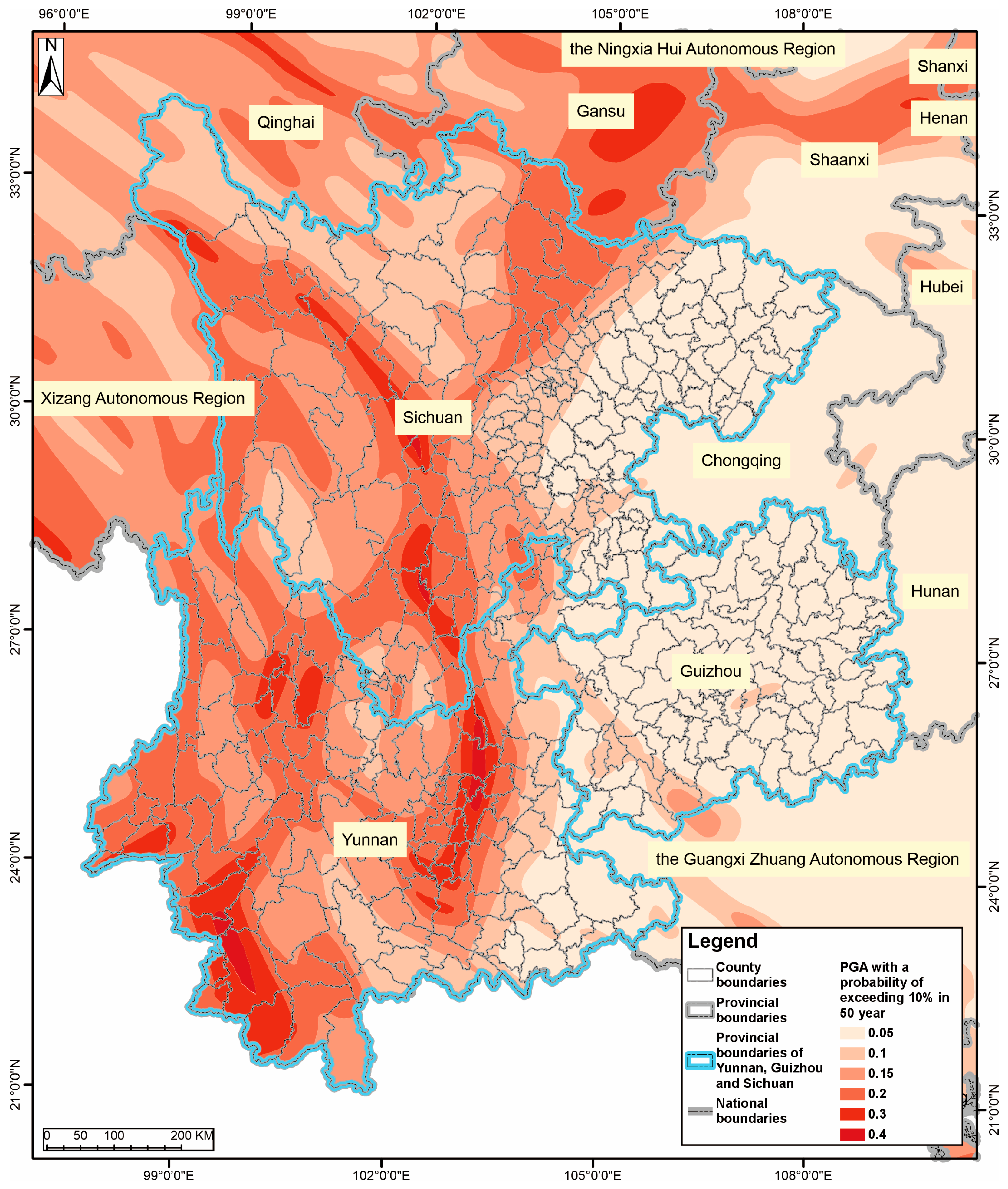
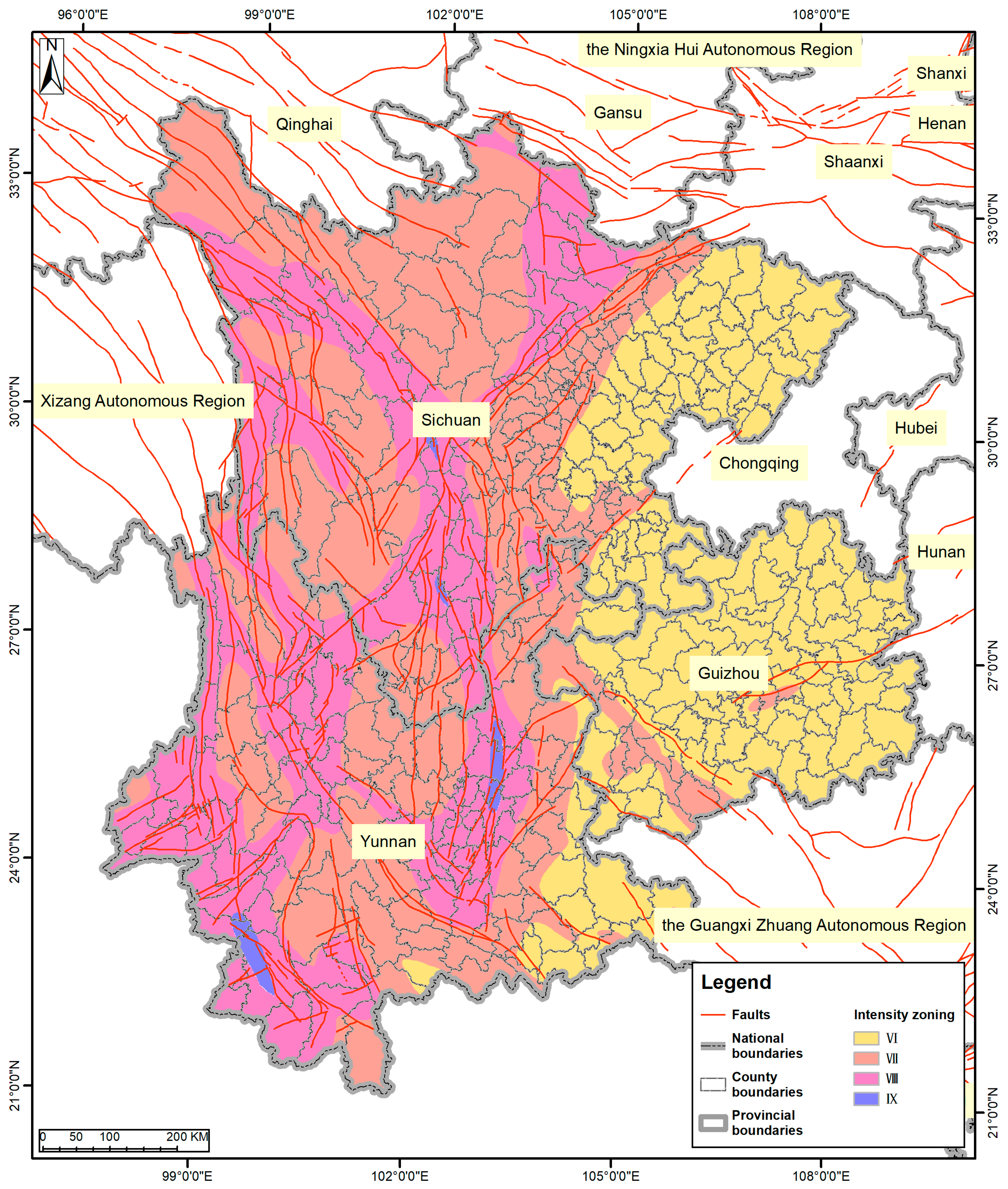
A standard [56] “Seismic Ground Motion Parameter Zoning Map of China” (GB 18306-2015) was released in 2016, detailing the basic ground motion PGA (peak ground acceleration) distribution (see Figure 4) and corresponding acceleration response spectrum characteristic period for class II sites in China, with a 50-year probability of exceedance of 10%. This standard also stipulates that the risk level of anti-collapse design parameters (rare ground motion) is not less than the 50-year exceedance probability of 2%, aligning with advanced countries in terms of earthquake prevention and disaster reduction. Utilizing the probabilistic seismic hazard analysis (PSHA) method proposed by [57], the zoning map employs active fault data (for instance, segmentation, length, and slip rate data of 243 fault segments from 130 faults, and paleoseismic data from 161 fault segments) to estimate the occurrence rate of large earthquakes. The PGA map is combined with the “Comparison table of site seismic peak acceleration and seismic intensity” (refer to Table 3), resulting in the 5th generation of seismic intensity zoning.
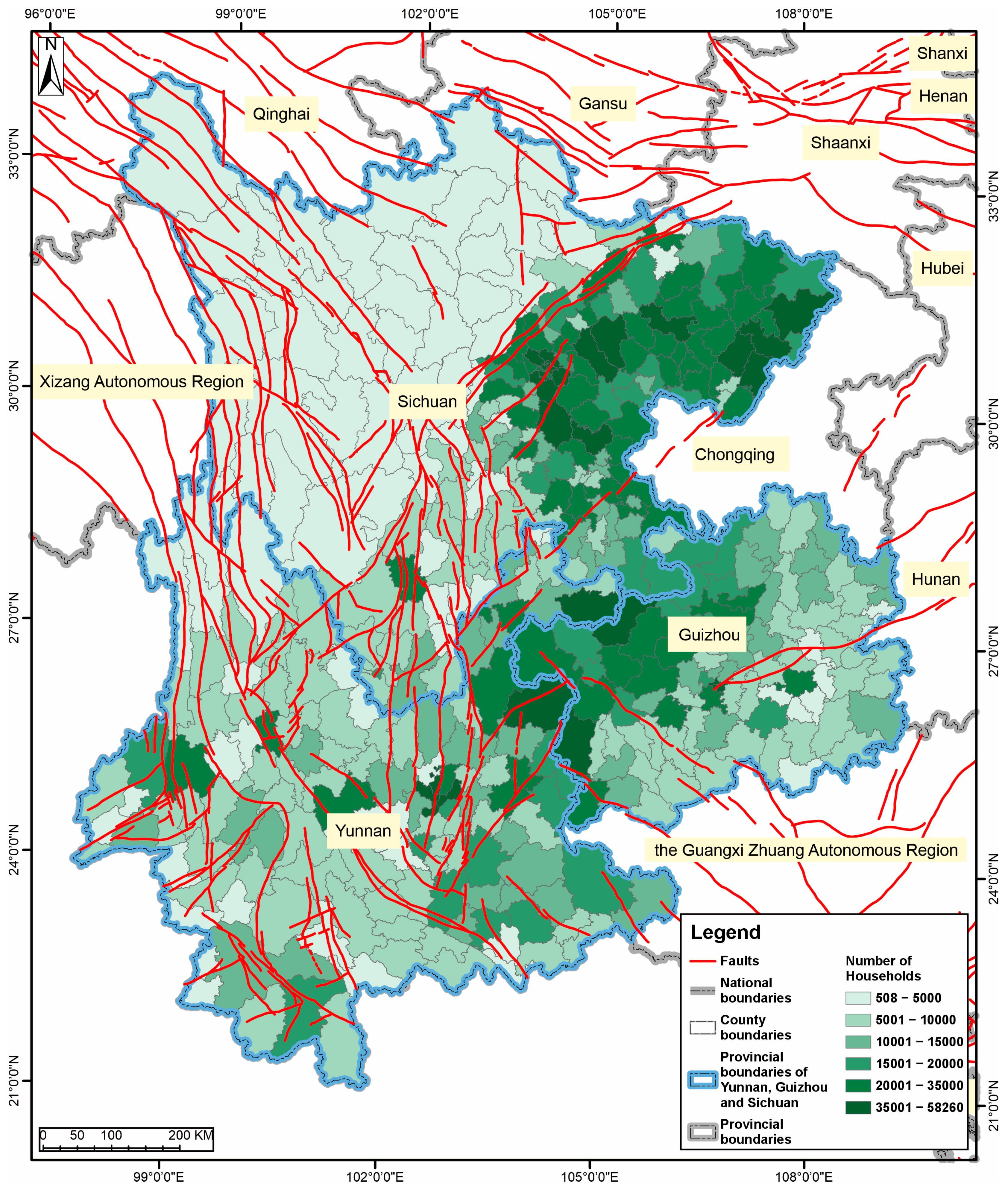
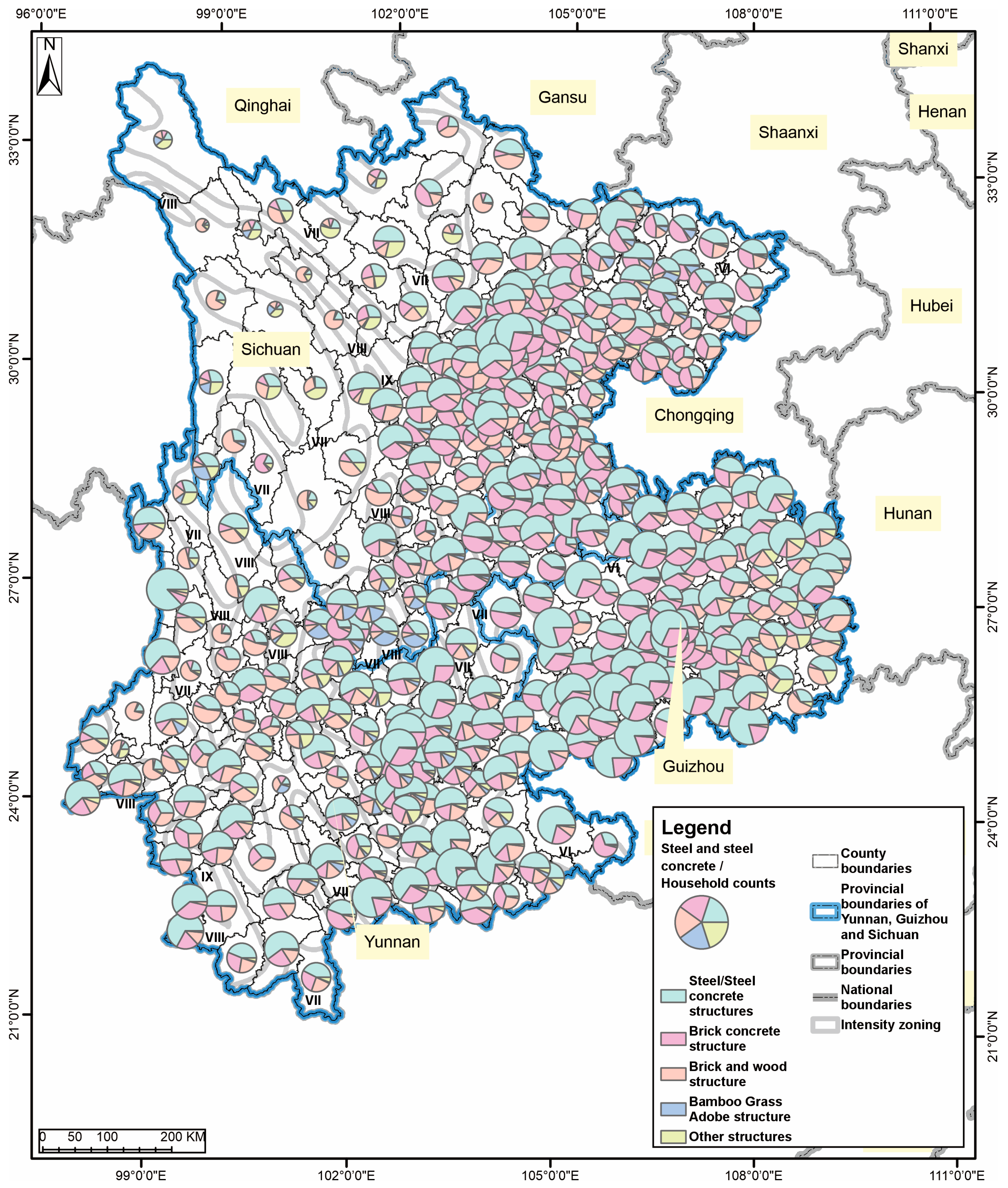
We utilized the household data from the census yearbook [51] (National Bureau of Statistics of China, 2025), which is categorized into five typical housing structure types or other attributes (refer to Figure 5 and Figure 6). The mapping relationship between building structure categories in the Seventh National Population Census Yearbook and the structural performance grades adopted in this study is established as follows: reinforced concrete structures correspond to the category designated as “reinforced concrete houses”; brick-concrete structures, brick-wood structures, and other masonry structures are collectively classified under “brick houses”; wooden structures correspond to “wooden houses”; earth-wood structures are mapped to “civil houses”; and bamboo, grass, or adobe structures correspond to the classification “bamboo/grass/adobe houses”. In the census yearbook, these families are classified into “summary”, “urban area”, “semi-urban area”, and “rural area” categories based on residence type, number of building floors, or bearing capacity type. Table 4, Table 5 and Table 6 present the counts and corresponding proportions of households classified by building structure in the urban, township, and rural areas of Chengdu City, Sichuan, China, based on data from the population census. Our data collection methods include: (1) obtaining permission to copy paper images [51,58]; (2) logging onto the official website of statistical institutions to request public information; (3) contacting the office of statistical institutions or the population division directly; (4) sending emails; and (5) employing other methods.
As shown in Figure 5, the residential distribution across the three provinces is uneven, with Sichuan being the most pronounced example. The residential density in the northeast is 2–10 times greater than that in the southwest. The Northeast Sichuan Plain is conducive to living and farming, resulting in relatively concentrated housing. In the central and western regions, as well as the northwest, the number of households in large areas ranges from 500 to 5000, while the southern region exhibits a more balanced distribution. Guandu District has 58,260 households, Chenghua District has 48,853, Shuangliu District has 46,757, and Jinniu District has 46,036, all exceeding 45,000. Notably, Xichang has the highest concentration of residents in the south with 27,361 households. The western part of Guizhou and northeastern Yunnan are flat and densely populated. The highest number of households in Yunyan District of Guiyang is 37,976, followed by 36,034 in Nanming District, 35,935 in Panzhou City of Liupanshui City, and 35,749 in Qixingguan District of Bijie City, all surpassing 35,000. In contrast, the residential areas in eastern and southern Guizhou are more scattered than those in the northwest, yet there are still some concentrated residential zones. Although the residential areas in Guizhou Province are predominantly in the northwest, the concentration is not as marked as in Sichuan. Among the three provinces, Yunnan has the most dispersed households, with the largest numbers in the western, central, and eastern counties, respectively: 58,260 in Guandu District of Kunming, 42,165 in Xuanwei City of Qujing, 38,867 in Wuhua District of Kunming, 37,675 in Zhenxiong County of Zhaotong, 35,901 in Xishan District of Kunming, and 34,461 in Panlong District of Kunming, all exceeding or nearing 35,000.
As depicted in Figure 6, the primary building structures in northeastern and southern Sichuan are reinforced concrete, with brick concrete and brick wood structures following. In the majority of the Chengdu Plain, over 50% of buildings are constructed with steel-concrete structures. Particularly in districts such as Jinjiang, Suining Hedong new area, Chengdu high tech Zone, and Deyang, the proportion of reinforced concrete houses exceeds 80%. In the Northeast of Sichuan, the prevalent building structure is brick concrete, followed by steel concrete. In areas such as Gong, Daocheng, and the West District of Panzhihua, the proportion of brick concrete structures exceeds 60%. In the mountainous regions of Western and Northern Sichuan, buildings are predominantly brick and wood structures, including civil structured and wood structures. Near the provincial boundaries of Gansu, Qinghai, and Tibet, over 60% of households are brick and wood. Specifically, in counties such as Daofu, Dege, and Baiyu, the proportion of brick and wood structures exceeds 60%, while the proportion of reinforced concrete ranges from 8.88% to 27.56%. In Huidong and Huili, the proportion of bamboo, grass and adobe houses exceeds 30%, with steel-concrete houses constituting 35.306% and 39.808%, respectively. In Lancang, Heishui, and Yajiang County, the proportion of civil structured and wooden houses exceeds 40%, while the proportion of steel-concrete structures is only 19.47%, 20.19%, and 25.86%. Overall, the total proportion of brick wood, civil, wood, bamboo, grass, and adobe structures in 41 counties in Sichuan exceeds 40%, and the provincial household ratio is 211,196/5,895,390, which equals 3.58%. Twenty-five counties, including Luhuo, Dege, and Xinlong, have a total proportion of brick, wood, civil, bamboo, grass, and adobe structures exceeding 50%. Notably, in eleven counties, including Luhuo, Dege, Xinlong, and Daofu, the proportion of reinforced concrete houses does not exceed 20%.
Figure 6 also depicts the distribution pattern of building structures in Guizhou Province. Drawing a north–south line from Guiyang, the provincial capital, reveals that most buildings in the western region are constructed from reinforced concrete and brick concrete. Notably, in the southwest, the proportion of brick wood, civil and wood structures is significantly lower. Specifically, in Guanshanhu, Bijiang, Wangmo, and Xingyi, over 80% of the houses are reinforced concrete. In Dafang, Xifeng, Xiuwen, Luodian, and Zhijin, more than 50% of the houses are brick concrete structures, and over 30% are steel concrete structures. On the eastern side of the line, reinforced concrete remains prevalent, but the proportion of brick wood, civil and wood structures has risen substantially, with some counties having more brick and wood houses than brick and concrete. In Congjiang, Danzhai, and Jinping, the proportion of brick and wood exceeds 40%, and the proportion of reinforced concrete exceeds 30%. Chishui is unique, with 14.38% of bamboo, grass, adobe, civil and wood structures, while steel concrete and brick concrete proportions are 34.78% and 41.63%, respectively. In Guizhou Province, Rongjiang, Jianhe, and Leishan have the highest proportions of civilian timber structures, all exceeding 20%. The proportion of brick timber structures is 23.873%, 24.98%, and 36.83%, respectively, and the proportion of steel-concrete structures is 38.13%, 40.60%, and 38.68%. Overall, except for Nayong, where the proportion of steel-concrete is 30.43%, and brick wood is 39.85%, and Congjiang, where the proportion of steel-concrete is 31.26%, and brick wood is 57.54%, the proportion of steel-concrete in other counties is more than 33%. The primary structures are steel-concrete and brick concrete, indicating that the overall level of building fortification design is relatively balanced. In Guizhou, there are 10 counties where the combined proportion of houses with brick, wood, civil, bamboo, grass and adobe structures exceeds 40%, including Congjiang, Rongjiang, Leishan, among others. The proportion of households in the province is 81,700/2,109,740 = 3.87%.
Except for a few counties in central and northern Yunnan, which are mainly brick and wood structure houses, other areas are predominantly reinforced concrete houses, followed by brick concrete and brick and wood structure houses. The proportion of brick and wood structures in nine counties, including Tengchong, Jianchuan, Longling, and others, exceeds 50%. The proportion of steel concrete in some counties, such as Fugong, Guandu, and Luchun, exceeds 70%. In some counties, civil structured houses and wooden structures also constitute a significant proportion. The proportion of civil structured and wooden houses in Yongsheng, Deqin, Lianghe, Wuding, and Nanhua County exceeded 20%, with the proportions in Yongsheng and Deqin reaching 35.936% and 30.719%, respectively. Overall, the proportion of residential houses, including wooden, bamboo, grass, and adobe houses, in 38 counties exceeded 40%, and the proportion of households in the province reached 434,527 out of 282,610, which is 15.38%. Among them, there are 23 counties, including Tengchong, Lianghe, Jianchuan, etc., where the proportion of brick wood, bamboo, grass and adobe structure houses exceeds 50%. Among these, the proportion of reinforced concrete houses in Tengchong, Lianghe, Jianchuan, and Jingdong does not exceed 20%.
Section 3.2 will introduce the anti-lethal level model, which is based on the results [18,52] (Xiwei, 2020; Gaochong et al., 2021). In this research, 52 historical fatal earthquakes from 1996 to 2010 were cited.

3. Methodology

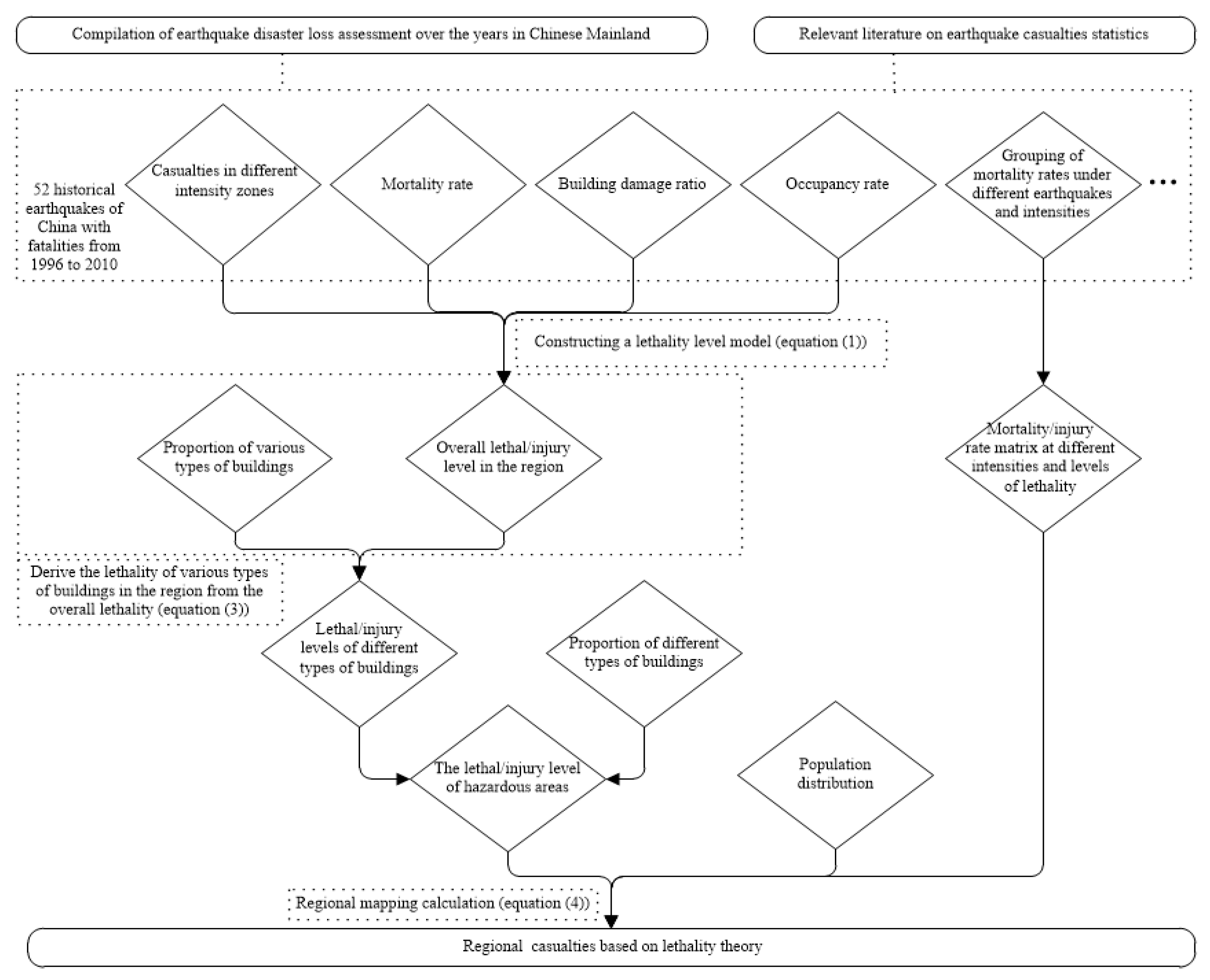
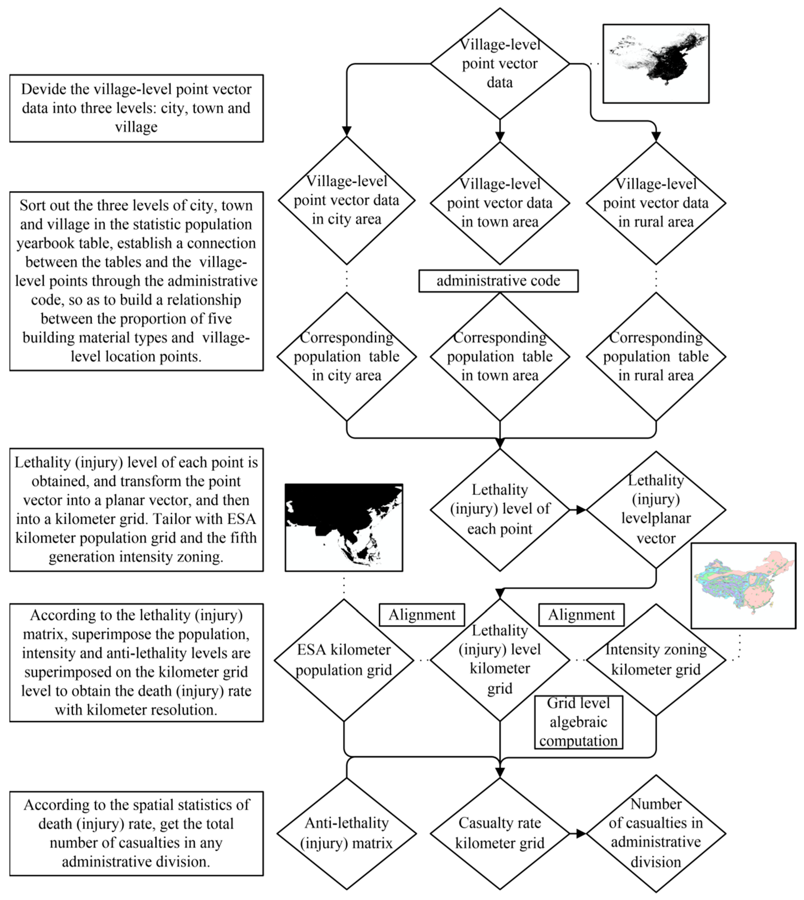
The specific steps of data preprocessing and region mapping calculation are shown in Figure 7: a rectangle represents the workflow, and a parallelogram represents the datum plane. After data preprocessing, the population, intensity zoning and anti-lethal level are superimposed according to the seismic matrix of historical earthquakes. Then, the mortality (injury) rate per kilometer grid in the intensity partition is determined by logical operation. On this basis, the kilometer level casualty rate spatial statistics were carried out to estimate the number of casualties in administrative divisions at all levels.

3.1. Data Preprocessing

The data point vectors of administrative villages are categorized into three groups based on their geographical positions. The urban and rural classification codes in the attribute table are defined according to the guidelines for the creation of statistical zoning codes and urban and rural zoning codes, as issued by the National Bureau of Statistics [59]. Each classification code consists of three digits, with the first digit “1” or “2” denoting urban or rural areas, respectively (refer to Table 7). In this document, data encoded as “111” and “112” are consolidated to represent urban areas, data encoded as “121”, “122”, and “123” are utilized to represent towns, and data encoded as “210” and “220” are employed to represent rural areas.
The Demographic Yearbook [58] classifies households by region, such as urban, township, and rural areas, and provides clear explanations (National Bureau of Statistics of China, 2022). Consequently, to map census data with building structure types, we categorize households based on the structure types outlined in the Yearbook, corresponding to the three administrative divisions of cities, towns, and villages. Next, we utilize the district/county administrative code to link the village/community vector data with the corresponding number of households for each building structure type. This connection allows us to establish a correlation between the locations of villages/communities and the distribution of housing types in these areas (see Figure 6), thereby aiding in the assessment of the local lethality of these locations.
This study integrates three categories of data aligned with kilometer-scale grid coordinates: demographic, intensity, and mortality datasets. Software including ArcGIS v10.2 was employed to conduct resampling of raw spatial data. Demographic data originate from the European Space Agency (ESA) kilometer-grid system. The construction of mortality kilometer grids follows a three-stage conversion procedure: from village- or community-level mortality polygon data to raster grids, and subsequently to kilometer-resolution grids. The overall workflow for generating kilometer-grid raster data from point vector data comprises three principal stages. First, point vectors are converted into polygon vectors (areal features) to facilitate the spatial dissemination of point attributes. The resulting polygons inherit all attributes from the original points (e.g., population size, administrative codes, total resources), with each polygon representing the unique attribute set of a corresponding village or community. Second, polygon vectors are transformed into raster data, with the target pixel size specified at the kilometer level during the vector-to-raster conversion. Resampling techniques are primarily applied during raster resolution transformation. When converting polygons to an initial raster dataset, a pixel size of 1000 m is designated. The core methodology involves discretely assigning attribute values from vector polygons to raster pixels using the Cell Center method: a pixel acquires the attribute value of the polygon within which its centroid is located; otherwise, a NoData value is assigned. To convert the initial raster data (e.g., higher-resolution data derived from polygons) into 1 km resolution grids, the ArcGIS v10.2 resampling algorithm applies the Nearest Neighbor method. This approach directly assigns the value from the source raster pixel corresponding to the center of each target pixel, without interpolation. The algorithm ensures computational efficiency while preserving all original raster attribute values, such as discrete attributes including village administrative codes and classification types. When polygonal feature attributes represent discrete data (e.g., township codes or land use type codes), the nearest neighbor method is optimal as it effectively prevents attribute distortion. The intensity zoning kilometer grid is generated from intensity vector surfaces using ArcGIS v10.2. During the conversion of vector surfaces to kilometer-grid raster data in ArcGIS, the core spatial sampling technique involves resampling with the default nearest neighbor method, which adopts the value of the source pixel closest to the target pixel centroid. This approach is suitable for discrete data types (e.g., land use categories and building classifications), as it preserves the original categorical attributes and prevents value distortion.
We summarize the grid alignment process steps for demographic, intensity, and mortality data as follows. (1) Establishing a unified spatial reference: employing the WGS84 longitude and latitude coordinate system with a grid resolution of 1 km × 1 km; defining grid coverage boundaries based on the study area extent (e.g., Yunnan, Guizhou, Sichuan) to prevent data clipping or overlap. (2) Collecting population data (from administrative unit statistics), lethality parameters, seismic intensity data (including PGA, PGV, and simulated China seismic intensity results), and building attribute data (e.g., type proportions and seismic resistance); standardizing data formats (such as Shapefile) and extracting spatial coordinate information. (3) Disaggregating administrative unit population data into 1 km grid cells based on remote sensing data and machine learning models (e.g., geostatistical regression): this achieves fine-grained population allocation from administrative units to grid units. (4) Resampling seismic motion parameter simulation results (e.g., PGA, PGV, typically in vector or high-resolution raster format) to 1 km grids: utilizing bilinear interpolation or Kriging interpolation methods to ensure spatial continuity of intensity parameters within grid cells; China seismic intensity data are transformed into rasterized intensity values in accordance with standards [56,60]. (5) Performing coordinate consistency checks on all data layers and correcting geometric deviations to ensure complete matching of grid boundaries and resolution, with an error tolerance of no more than 0.5 grid cells. (6) Integrating population density, intensity parameters, and building type proportions within unified grid units, ensuring precise spatial alignment among population distribution, lethal factors (specifically building vulnerability), and intensity parameters within the same grid unit. (7) Eliminating outliers, such as unreasonable grids with population density exceeding 5000 people/km2, to maintain data consistency.
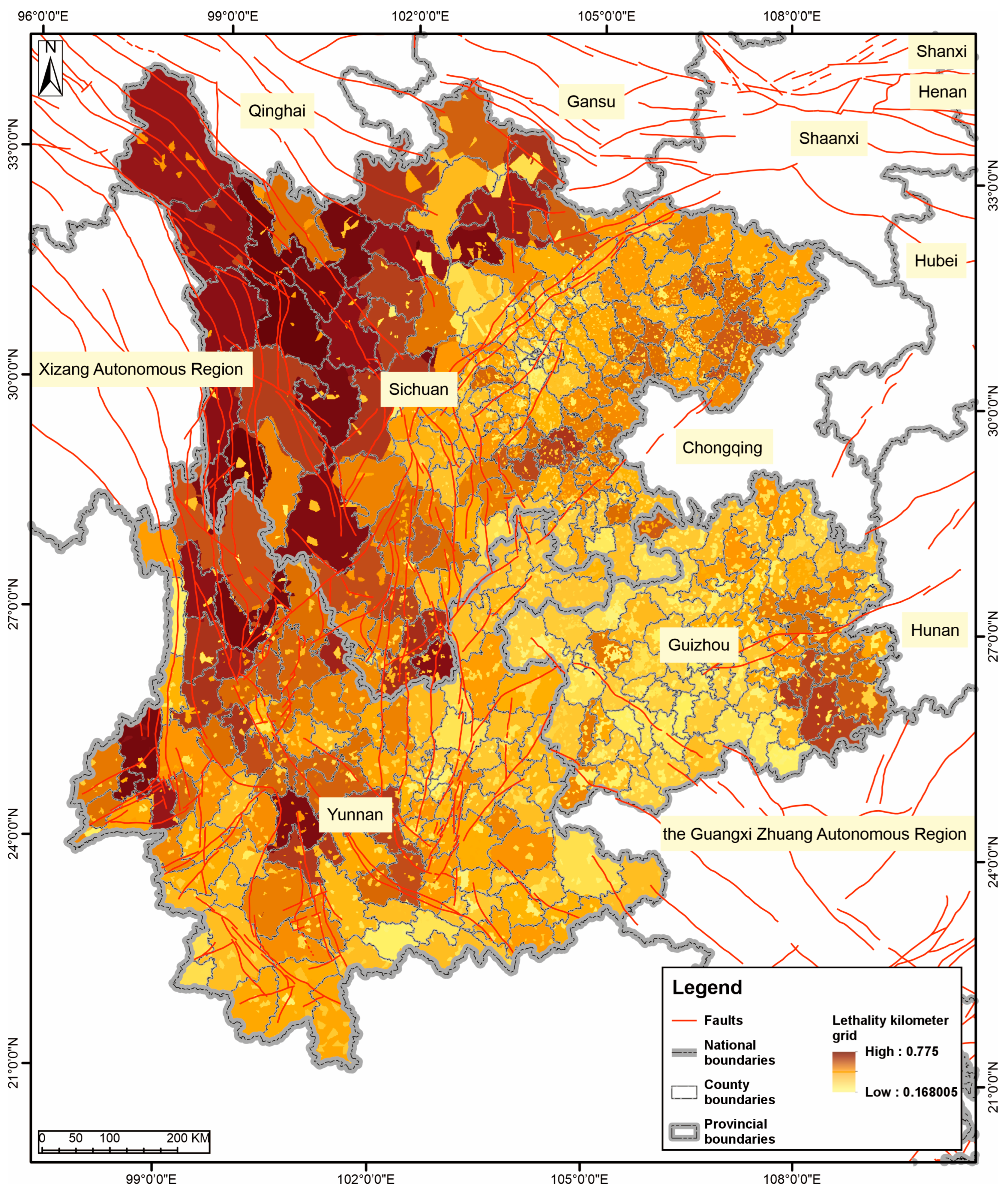
By analyzing the proportion of housing types at village points, the anti-lethal level of these villages/communities can be determined by proportionally weighting the anti-lethality of each structure type. Subsequently, the location of the village/community is converted into a Voronoi polygon surface vector through neighborhood analysis, and ultimately, it is transformed into a regular kilometer grid with a feature of lethality based on the pixel center principle. Furthermore, when the seismic intensity zoning in China is converted into a grid and tailored to the study area (Figure 8), the grid level is precisely aligned with the ESA population grid (Figure 9) and lethality grid (Figure 10) on a spatial scale of kilometers.
Seismic intensity zoning is closely related to the distribution of faults, which is inseparable from the methodology for determining seismic intensity zoning [56]. As illustrated in Figure 8, Kangding, Luding, and Xichang along the Xianshuihe fault, Anning River fault, and Zemuhe fault in central and southern Sichuan, as well as Songming, Yiliang, Xundian, and Dongchuan along the Xiaojiang Fault in eastern and southwestern Yunnan, and Lancang, Cangyuan, and Gengma along the Longling Lancang fault, are located within the IX seismic intensity zone (colored blue-purple), indicating a probability of occurrence exceeding 10% within a 50-year period.
High seismic intensity areas do not always align with regions of high population density. As illustrated in Figure 9, Panlong and Guandu are adjacent to Songming County, situated within the IX intensity zone and hosting the highest population density in Yunnan Province, reaching up to 100,000 people per square kilometer. However, counties such as Lancang, Cangyuan, and Gengma, also within the IX intensity zone, exhibit a relatively low population density, not surpassing 1000 people per square kilometer. A similar pattern is observed near the Xianshuihe fault in Sichuan, where the population density remains low, not exceeding 500 people per square kilometer. In contrast, the population is more concentrated near the Anning River and Zemu River, with the highest density occurring near the Zemu River, exceeding 17,000 people per square kilometer.
Chinese residents are predominantly concentrated in urban areas, with 63.89% residing in cities and towns, while the remainder is relatively dispersed across rural regions [58] (National Population Statistics Yearbook, 2022). The level of economic development determines that housing in urban areas has higher seismic performance, so high earthquake mortality often avoids areas with high population density. Our mortality model is primarily based on the proportion of local building structures and the lethal levels of each type. Consequently, the lethality of earthquakes is closely linked to the seismic fortification standards of local residences. The sparsely populated regions of Western Sichuan, Western Yunnan, and Eastern Guizhou exhibit high lethality, a fact that is illustrated in Figure 9 and Figure 10.

3.2. The Anti-Lethality/Anti-Injury Matric

Drawing upon the lethality theory, refs. [36,37] proposed a semi-empirical assessment method based on building vulnerability. The model is constructed via the statistical fitting of the relationship between building vulnerability and fatalities, and it does not belong to the category of empirical function methods that rely on parameters such as seismic parameters and population density. Figure 11 illustrates the Methodological flowchart depicting the construction of the lethality/injury matrix (vulnerability) and its interaction with intensity parameters (hazard) and human population (exposure) grids in this study. Through an analysis of historical records of fatalities in different seismic magnitudes and intensity zones across various regions of China, two relationship characteristics among seismic magnitude, intensity, and mortality rates were summarized:
(1)
There is a multiple-relationship characteristic between the mortality rates of adjacent intensity groups. In this study, by summarizing over 30 historical earthquakes in China, the earthquake mortality rate (ranging from 0% to 30%) and probability (ranging from 0% to 100%) were respectively employed as the horizontal and vertical axes. The probability of mortality rates occurring within the 0–30% range corresponding to seismic intensities from VI to XI degrees was fitted. An empirical multiple relationship of 2:4:14:32:39:32 was obtained based on the standard deviations between adjacent intensity groups. Subsequently, the mortality multiples for adjacent intensity groups (VI–VII, VII–VIII, VIII–IX, IX–X, X–XI) across all historical earthquakes from VI to VIII degrees were plotted on the horizontal axis, with probability on the vertical axis, to acquire the discrete distribution of mortality multiples (ranging from −20 to 50) and probabilities (ranging from 0% to 100%) for all historical earthquakes. This process facilitated the fitting of curve slopes, namely, the slope of the historical earthquake fitting curve.
(2)
The mortality rates of individuals at different seismic intensity groups demonstrate distinct exponential relationships and grouping phenomena. In this characteristic, by summarizing the relationship between intensity (from degree VI to XI) and mortality rate (0–3%) of over 40 historical earthquakes in China and normalizing the correlation curves, it was found that the normalized intensity–mortality rate curves of these historical earthquakes naturally clustered. This suggests that the mortality rates of historical earthquakes in China exhibit natural grouping phenomena across different intensity levels, which can be classified into 11 mortality rate groups; this constitutes the core of the theory: 11 lethality level classifications.
Following characteristic (2), it is logically inferred that there is a corresponding relationship between the slope of historical earthquake fitting curves, lethality level classifications, and mortality rates. Finally, refs. [36,37] constructed a matrix and evaluation model based on lethality level grades and intensity-specific mortality rates, which reflects the content of Equation (7).
By analyzing historical earthquakes, the overall anti-lethality level of a region can be evaluated. This theory establishes a field investigation lethality level model through field surveys. For example, geological and geomorphological factors are classified into three influencing elements: determining whether the study area contains faults, with the distances to fault zones being less than 50 km, greater than 50 km, or having no fault zones at all; identifying the presence of steep slopes (slope angle > 10 degrees), gentle slopes (slope angle < 10 degrees), or flat terrain (no slope gradients); and analyzing slope characteristics. Taking Equation (2) as an illustration, if the weight of the geological and geomorphological factor is ω i , the distribution of fault zones serves as a secondary geological and geomorphological factor with a weight of ω i j , while the presence of faults acts as a tertiary factor with a weight of ω j k .
The lethal level varies with seismic intensity, which is a relative index influenced by the type, proportion, material, quality, and construction method of the building structure. Fundamentally, the lethal level for each building type must be determined based on its specific influencing factors. For comparable buildings, the lethal value should fall within a specified range [36,37].
Upon acquiring the lethality level through field investigations, the lethality levels of diverse local buildings are inversely deduced from the overall lethality level. This procedure employs parameters including architectural structures, foundation types, construction dates, usage purposes, and the lethality levels of residential buildings within the surveyed region. The range of the anti-lethality level for each building type can be determined by constructing and solving a multivariate first-order formula (refer to Table 8).
By utilizing historical earthquake casualty data corresponding to various seismic intensities (linked to Peak Ground Acceleration and Peak Ground Velocity), we establish the correlation between mortality/injury rates and seismic intensity within the lethality matrix. Based on casualty patterns derived from historical earthquakes in distinct regions (e.g., Southwest and Northwest China), we calibrate region-specific lethality matrices. Through comparative analysis of actual historical earthquake casualties and model-predicted casualties, we iteratively optimize the parameters of the lethality matrix to improve the precision of casualty assessment. By leveraging historical seismic data, the validation of mortality coefficients was supplemented as presented in Table 9.
After identifying the factors influencing regional lethality and determining the weight ratio of each factor in the first and second levels of classification, the overall lethality model can be constructed using the weight ratio coefficients of each factor, as depicted in Equation (1) [6,41,61,62,63,64,65]. Furthermore, the regional lethal level coefficient adjustment model is presented in Formula (2) [6]. For the definition of each parameter, refer to [6,36,37,41].
In this model, the 11 levels of lethality ranged from 0 to 1. The anti-lethal/anti-injury matrix is generated according to the intensity levels VI to XI. Intuitively, the horizontal axis and the vertical axis represent the earthquake intensity and anti-lethal/anti-injury levels respectively, pointing to the unique casualty rate value. Therefore, to understand the lethal level of an area, we can directly refer to the casualty rate, and the error is guaranteed to be within ±50% [36,37].
l o g R D = 12.479 P t · ρ · R A · α 0.1 13.3
a d j u s t = i = 1 3 ω i · ω i j · ω j k 1

3.3. Calculation

Initially, we calculate the proportion of households residing in various building structures at the county/district level using the specific household numbers from the census data. Subsequently, we apply these ratios as coefficients and integrate them with the anti-lethal/anti-injury levels of each structure type to ascertain the county/district-level overall anti-lethal level. As outlined in Section 3.1, we link the anti-lethal/anti-injury table of each county/district to the village vector attribute based on the administrative code, ensuring that each village/community is assigned a distinct value. The primary objective when integrating data from various sources is to convert county-level household statistics into kilometer-level data. This conversion allows us to correlate the data with population density and intensity for further analysis. However, since the intensity division relies on plane vector data, it must be transformed into grid format while preserving its fundamental characteristics. It is crucial to maintain the consistency of the coordinate system and use the target area as a template. When creating a raster, accurate edge capture is essential. Additionally, because the population data are in grid format, they must be trimmed to fit the boundary of the target area. Emphasis should be placed on the coordinate system to ensure that the edges are aligned with the edges of other data by-products. After aligning the data, each grid becomes our target, allowing us to calculate the matrix by stacking earthquake intensity zoning (Figure 8), population distribution (Figure 9), and lethal level (Figure 10). Based on the mortality and population size corresponding to the overall lethal level in the region, the mortality/injury estimation model is established. The anti-lethality/anti-injury matrix introduced in Section 3.2 is then applied to perform the conditional allocation operation for each grid. If the criteria of earthquake intensity and lethality are met, the mortality/injury rate is determined. Finally, through spatial analysis, such as multiplication with the population, the number of casualties in each administrative region is estimated through aggregation.
The prepared data in this study of the logical operational approach regarding the casualty rate within grid cells comprises: spatial population data (e.g., 1 km × 1 km) measured in population density (people/km2), building structure types and their proportions (including brick, wood, earth, bamboo-straw adobe, brick-concrete, reinforced concrete, etc., presented as percentages); peak ground acceleration (PGA) of grid cells, China seismic intensity (in accordance with standards [56,60]), etc.; regional fatality/injury matrices: basic fatality matrices constructed based on study regions (such as the southwest and northwest) with seismic motion parameters (e.g., PGA, seismic intensity) as indices (%). Operational calculation steps include the following:
(1)
Acquire the peak ground acceleration (PGA) or seismic intensity values of grid cells via seismic motion simulation (in conjunction with rapid reporting information and real-time social perception data), which serve as key indices for matching regional fatality/injury matrices.
(2)
Based on the location area of the grid cell (e.g., a sub-region in Sichuan, Yunnan, Guizhou), access the corresponding “regional fatality/injury matrix” and utilize the seismic motion parameters obtained in Step 1 (e.g., PGA = 0.2 g or seismic intensity VIII degree) to retrieve the basic mortality rate of the grid cell (in percentage) L0.
(3)
Compute the structural fragility coefficient V according to the proportion of different building structures within grid cells:
V = i = 1 n ( P i × V i )
where P i denotes the proportion of structural types in category i (e.g., 30% for brick structures, hence P i = 0.3 ), and V i represents the fragility weight of category i structures (based on seismic performance surveys of regional buildings: V i = 1.5 for bamboo-wattle adobe houses and V i = 0.3 for reinforced concrete buildings, with higher values indicating greater fragility). The adjusted mortality rate is calculated as L 1 = L 0 × V .
(4)
Using spatialized population density data (D, people/km2) from grid cells, calculate the total population within the cell N = D × S (where S denotes grid area; e.g., S = 1 for 1 km2).
(5)
The casualty rate R (%) of the grid cell serves as a comprehensive metric that combines adjusted mortality rates and population distribution N e x p o s e d denotes the actual population exposed to seismic risk within the grid cell (with a default value of [value not provided N ], which can be adjusted according to diurnal population dynamics).
R = L 1 × N e x p o s e d N  
(6)
Considering the nonlinear relationship between casualties and Peak Ground Acceleration (PGA), a nonlinear correction coefficient K should be employed when PGA or seismic intensity surpasses the threshold (e.g., PGA > 0.3 g). (Based on historical data fitting, for instance,
K = 1 + 0.5 × ln ( P G A / 0.3 )
The final case mortality rate was adjusted by quation
L f i n a l = L 1 × K
The values are substituted into Step 5 to compute the casualty rate. The casualty rate R (%) of a grid cell denotes the proportion of estimated casualties within that cell relative to the total population.
In Equation (7), D d represents the number of deaths, m is the anti-lethal level, defined as 1 minus the lethal level, n represents the seismic intensity, and L m n and D m n correspond to the mortality rate and population size of the area with the intensity of n and the lethal level of M [6,61,64].
D d = m = 0 1 n = V I X I L m n · D m n

3.4. Sources and Validation of Casualty Estimation Errors: An Analysis of Allowable Error Thresholds

The uncertainty inherent in casualty predictions generated by models primarily originates from three categories of errors: data input errors, model parameter errors, and model structural uncertainties. Specifically:
(1)
Data input errors encompass spatialization inaccuracies in demographic data and imprecisions in building typology data. While spatialized population data can improve accuracy, contemporary population statistics frequently depend on administrative divisions (e.g., county-level units), resulting in uneven spatial distributions at grid scales (e.g., 1 km × 1 km). Assuming that interpolation errors for population density adhere to a normal distribution, a standard deviation σ 1 of approximately ±30% corresponds to common error ranges observed in remote sensing-derived population data (e.g., errors from nighttime light interpretation or sample surveys). In southwestern China, brick-wood and earth-wood structures constitute over 50% of the building stock, whereas reinforced concrete structures represent less than 20% (Conclusion 5). However, county-level statistical classifications may demonstrate ambiguity (e.g., indistinct boundaries between “brick-wood” and “earth-wood” structural categories), introducing errors in seismic performance parameters. A uniform distribution error range of ±25% σ 2 is assumed.
(2)
Model parameter errors, specifically the uncertainty associated with regional mortality/injury matrices. Existing matrix parameters are derived from limited samples (e.g., an insufficient number of historical earthquake cases), inducing biases in mortality-intensity relationships (such as those between peak ground acceleration and casualty rates). The standard error of parameter estimation is assumed to be σ 3 approximately ±30%, based on t-distribution errors arising from small-sample statistical inference.
(3)
Model structural uncertainties, which may involve the underestimation of secondary disasters and soft impacts. The model does not comprehensively incorporate secondary disasters such as landslides and rockfalls, nor does it account for indirect losses stemming from public opinion dynamics. These omissions may result in an underestimation of casualties by 10% to 20%. A systematic bias of σ 4 approximately ±20% is therefore assumed.
Applying the root mean square error propagation theory (which superposes independent error sources), the total standard deviation σ t o t a l is calculated as the square root of the sum of the squares of all individual error sources (Equation (8)):
σ t o t a l = σ 1 2 + σ 2 2 + σ 3 2 + σ 4 2
Upon substituting the aforementioned error values and accounting for the non-normal distribution of errors, as exemplified by the uniform distribution of parameter errors, the actual total error σ a l l range undergoes a slight narrowing, ultimately converging to ±50% (Equation (9)).
σ a l l = ( 0.3 ) 2 + ( 0.25 ) 2 + ( 0.3 ) 2 + ( 0.2 ) 2 = 0.09 + 0.0625 + 0.09 + 0.04 = 0.2825 0.53 , ( ± 53 % )  
By employing 10,000 Monte Carlo simulations, random sampling was executed for various error sources: population error ( N ( 0 ,   0.3 2 ) ), building data error ( U ( 0.25 ,   0.25 ) ) , parameter error ( N ( 0 ,   0.3 2 ) ) , and structural error ( N ( 0 ,   0.2 2 ) ) . The simulation results indicated that the 90% confidence interval for predicted casualties spanned a r [ 48.7 % ,   + 51.2 % ] ange encompassing ±50% of the total variation, thereby validating the rationality of the error margin. International earthquake casualty prediction models, such as FEMA HAZUS and the European SHARE model, typically demonstrate error margins of ±40% to ±60% in data-scarce developing countries, as evidenced by post-2008 Wenchuan earthquake model validation. The study area, encompassing Yunnan, Guizhou, and Sichuan, is characterized by low seismic resistance in buildings and sparse data availability. The ±50% error range obtained in this study is consistent with findings from comparable research.

4. Result

4.1. Casualty Assessment Under a Basic Ground Motion Level

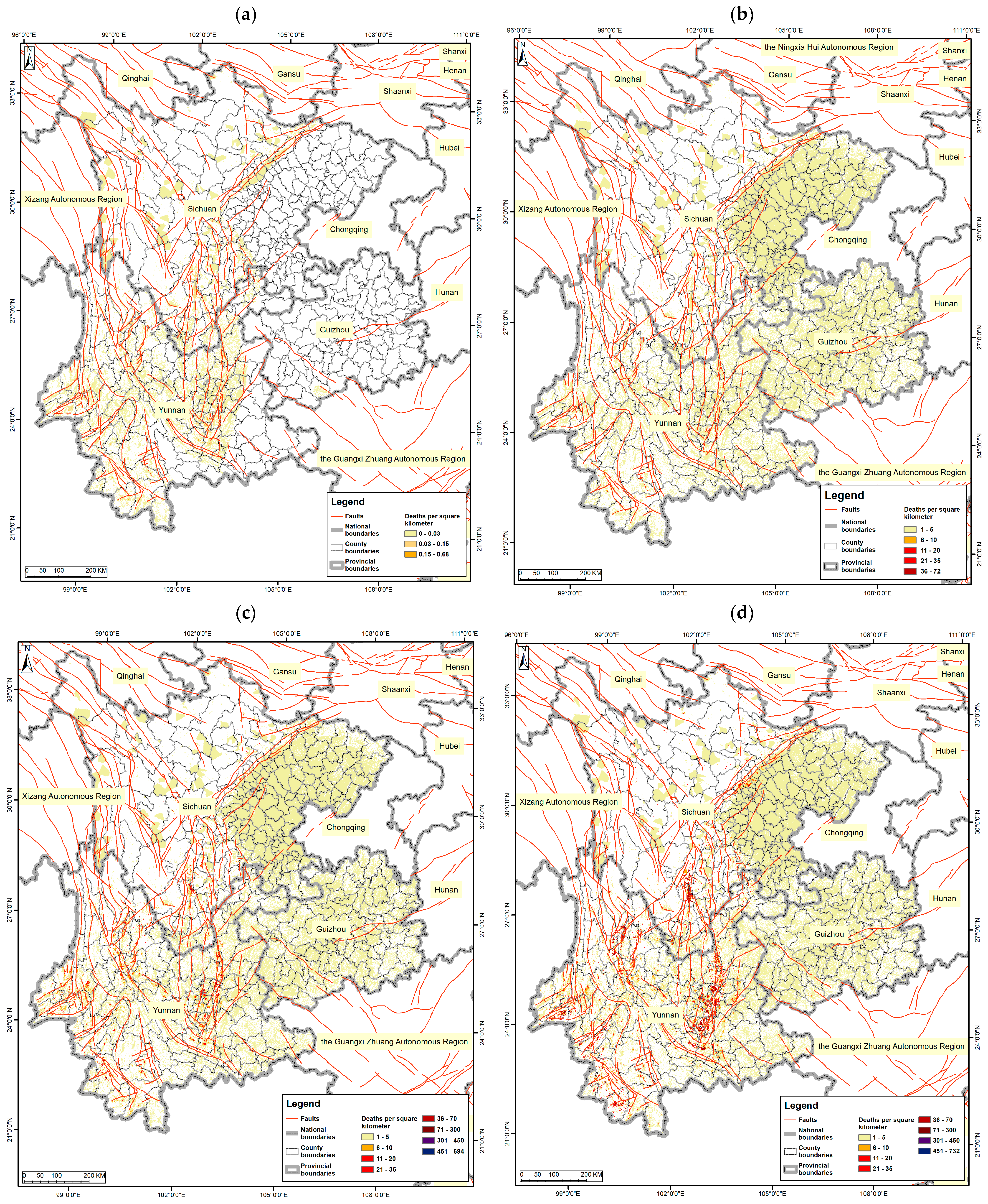
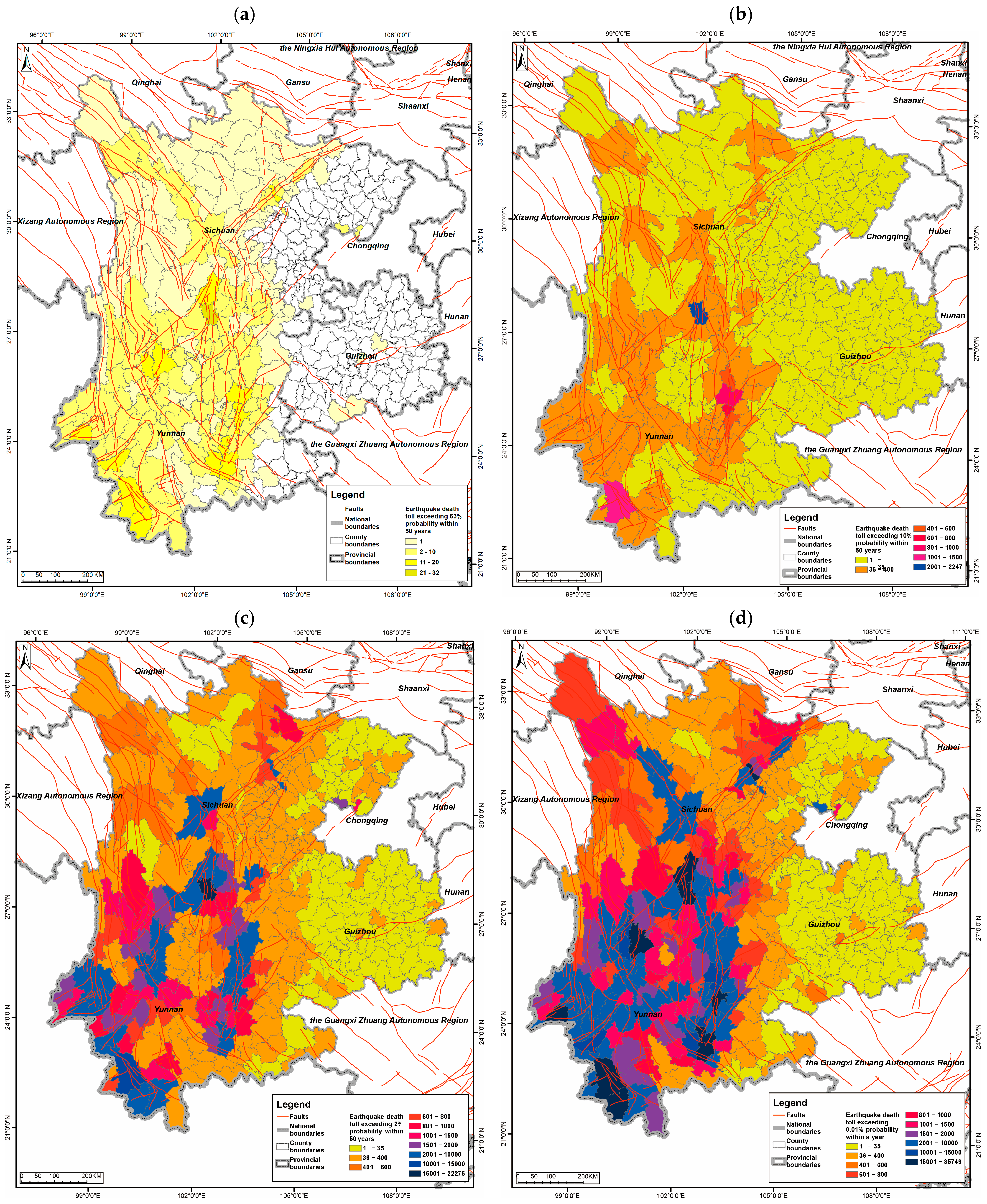
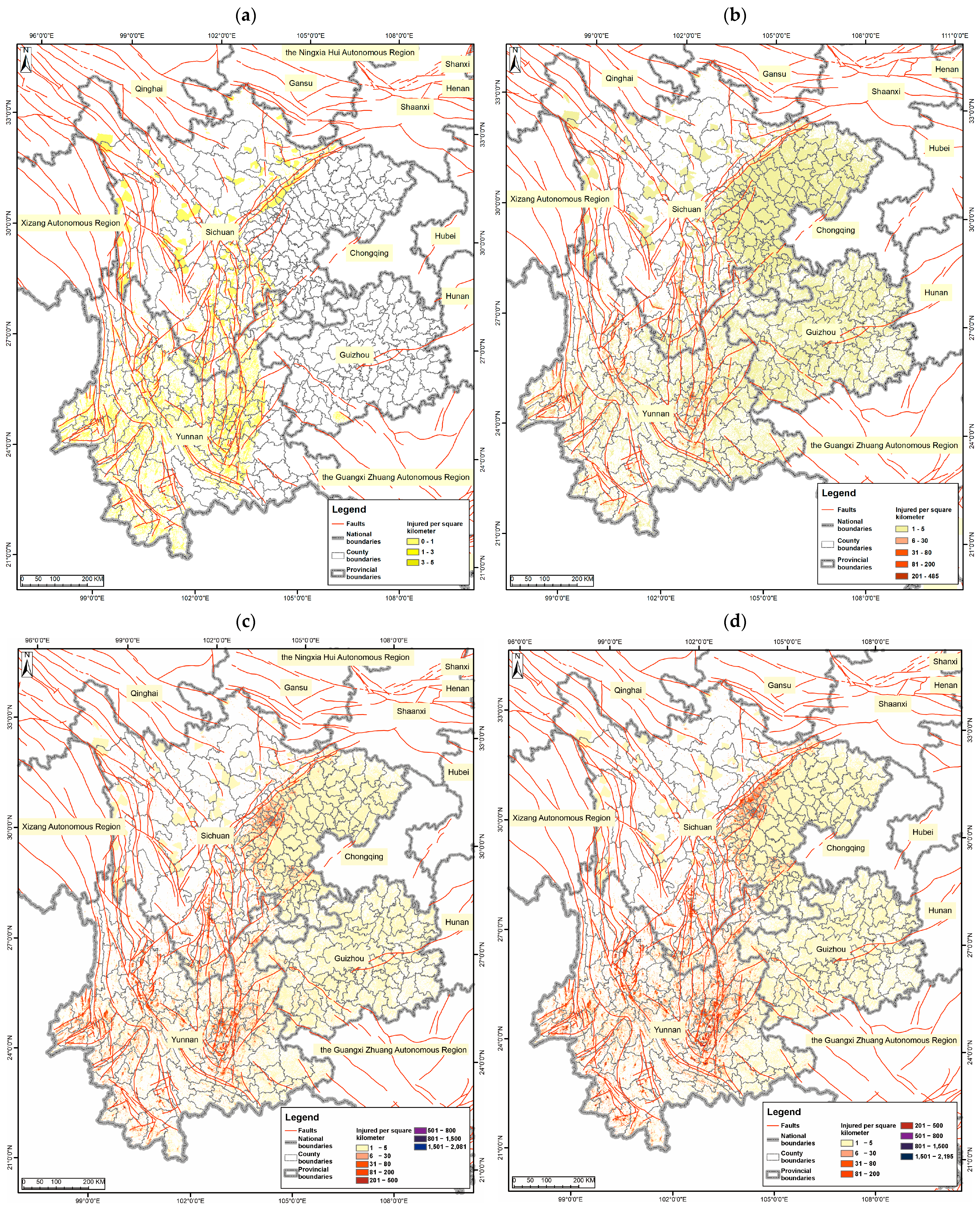
Our initial focus is on regions where casualties are concentrated, employing the method detailed in Section 3.3 to derive earthquake casualty assessments for southwestern China. Figure 12b and Figure 14b depicts the assessment of fatalities and injuries with a PGA probability exceeding 10% over a 50-year period. Upon comparing Figure 8, Figure 9, Figure 12b and Figure 14b, it becomes evident that since casualty numbers are calculated based on a population grid matrix, the distribution of casualties inherently relies on population density. Nonetheless, it is clear that the intensity of ground motion alone cannot fully dictate the density of casualties; the lethality level must also be taken into account. Thus, the distribution of casualties largely hinges on these fundamental factors: the intensity of the disaster, the resilience of the affected population, and the extent of population exposure.
Figure 12b and Figure 14b show macroscopically that the regions with the highest casualty density in Sichuan are located in the southern and central eastern areas. Given the vast territory and sparse population of the Chuanxi Mountain region, the distribution of casualties is extremely scattered. Apart from the northwest and southeast of Yunnan, where the casualty density per kilometer is relatively low due to sparse population or less fault activity, the distribution of casualties in other areas of Yunnan is uneven and varies significantly. With the exception of a few residents in the eastern and western mountainous regions, the distribution of residents in Guizhou is relatively even, and the casualty density is generally low, mostly between 1 and 5 per square kilometers.
To understand the distribution of county-level casualties in southwestern China, we utilized a regional geometric analysis method to obtain the total, ranking, average, and standard deviation of grid casualties within each county partition (Figure 13b and Figure 15b). Table 10 and Table 11 present the casualty assessment for various counties in southwestern China, indicating a probability exceeding 10% within the next 50 years.
When the 50-year PGA exceedance probability reaches 10%, Xichang is estimated to incur 2247 fatalities and 17,297 injuries. With a population of 817,282, this translates to a mortality rate of 0.27% and an injury rate of 2.12%. Lancang Lahu Autonomous County, with a population of 540,469, is projected to have 1243 deaths and 9863 injuries, resulting in mortality and injury rates of 0.23% and 1.82%, respectively. Counties with estimated death tolls ranging from 300 to 1000 include the Xundian Hui and Yi Autonomous Region, Songming, Dongchuan, and others. Three counties—Xundian, Songming, and Dongchuan—have a combined death toll of 2170, with individual counts between 500 and 999. 44 counties report 100–499 deaths, summing up to 7420 people. Additionally, 159 counties experience 10–99 deaths, totaling 5202 people. In 192 counties, there are fewer than 10 deaths, with a combined total of 578. Counties expected to have between 5000 and 9000 injured persons include Tengchong, Longyang, Xundian Hui and Yi Autonomous Counties, among others. In seven counties, 49,188 people have been injured, with the number of injuries ranging from 5000 to 9999: Lancang, Tengchong, Longyang, and others. The number of injured people in 47 counties ranges from 2000 to 4999, totaling 141,236 people. A total of 37,628 cases are reported in 26 counties. In 26 counties, 20,285 people are injured, with the number of injuries ranging from 500 to 999. In 65 counties, 14,553 people are injured, with the number of injuries ranging from 100 to 499. In 228 counties, 5746 people are injured, with the number of injuries being less than 100. By calculating the area of each county, we determine the death toll per square kilometer. Seven counties have a death toll exceeding 0.5 people per square kilometer, and 2 counties have a death toll exceeding 1 person per square kilometer, namely Xichang and Songming. The county with the highest number of injuries per square kilometer is still Xichang, with 20 people. There are three counties with a casualty density of 10–20 persons/km2: Wuhua, Panlong, and Songming, with Wuhua covering an area of only 255 km2. There are 101 counties with a casualty density of 1–9 persons/km2. Across Yunnan, Guizhou, and Sichuan, with a combined population of 179,196,903, the estimated fatalities are 18,861 and the estimated injuries are 285,938, leading to a total mortality rate of 0.011% and a total injury rate of 0.16%.
A Chinese national standard [66] GB/T 29425-2012, establishes the unified basis, activation conditions, and disposal requirements for the classification of emergency responses in China, thereby providing a consistent framework for action to governments and departments at all levels. This standard specifies that, as a category of natural disaster, earthquake events necessitate the classification of emergency response levels based on a comprehensive assessment of factors including casualties, property losses, social impact, and disaster relief capabilities, with casualties serving as the core criterion. Specific thresholds should be formulated through differentiated standards tailored to local conditions, such as economic development levels and disaster relief capacities; the standard does not separately prescribe explicit casualty thresholds for earthquakes. In light of this framework, and according to the National Earthquake Emergency Plan issued by the General Office of the State Council in 2020, earthquake disasters are categorized into four distinct levels: (1) particularly serious earthquakes that result in over 500 fatalities in key areas or those with a magnitude of 7.5 or greater; (2) major earthquakes causing 100–500 deaths or those with magnitudes ranging from 7.0 to 7.5 in key areas; (3) significant earthquakes resulting in 10–100 deaths or with magnitudes between 6.0 and 7.0 in key areas; and (4) general earthquakes causing fewer than 10 deaths or with magnitudes between 5.0 and 6.0 in key areas. The corresponding emergency response is classified into four grades: I, II, III, and IV. Based on our assessment and the earthquake emergency plan, we have identified counties with a likelihood exceeding 10% of reaching the first level of earthquake emergency response withover a 50-year period, including Xichang, Lancang, Xundian, Songming, and Dongchuan (refer to Table 10 and Table 11).

4.2. Earthquake Casualty Assessment with Various PGA Exceedance Probabilities

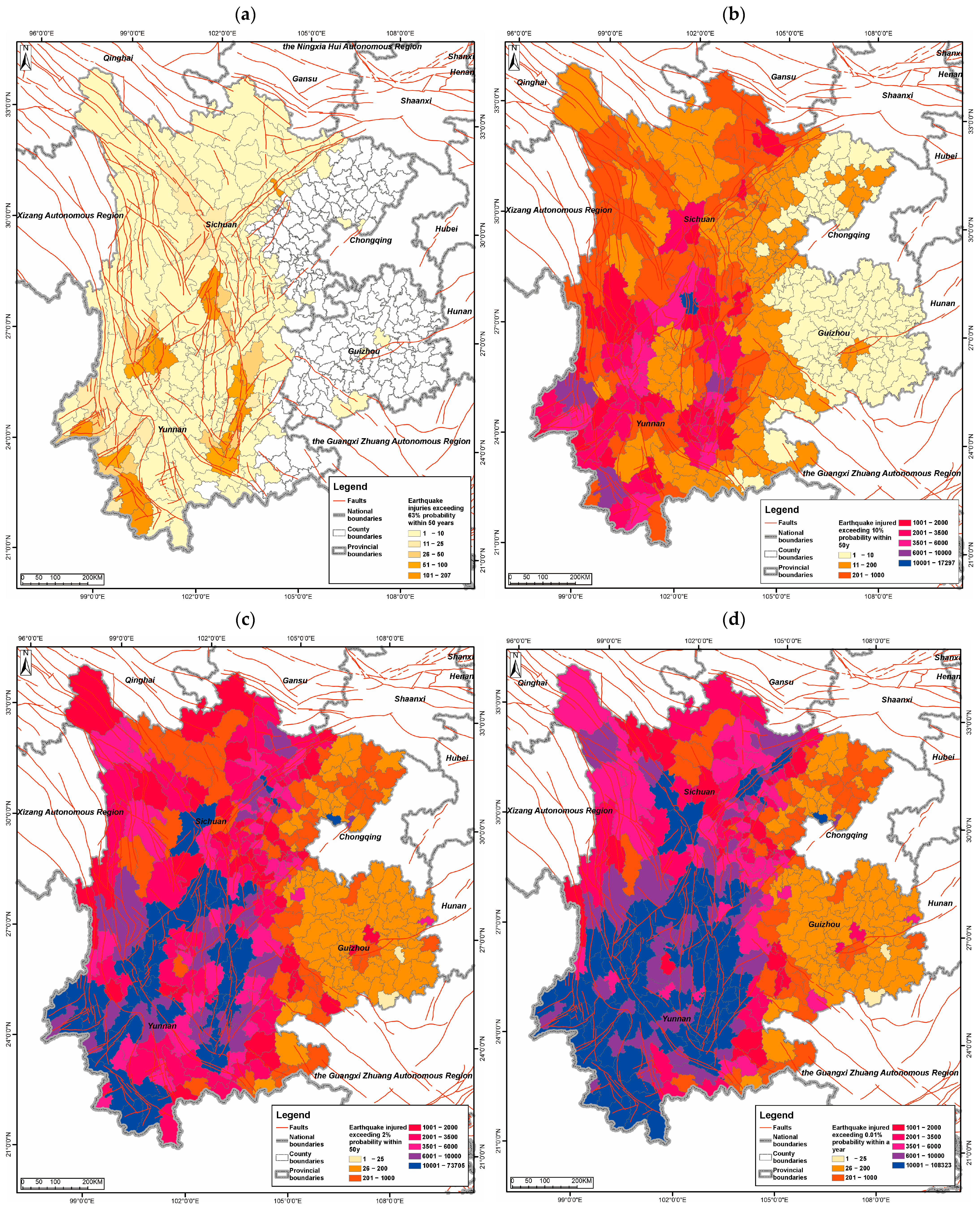
According to standard [56], ground motions with a 50-year probability of exceeding 10% are classified as basic ground motions. The peak acceleration of frequent ground motion should not be less than one-third of the basic peak acceleration of ground motion; the peak acceleration of rare ground motion should be 1.6-to-2.3 times the basic peak acceleration of ground motion; and the peak acceleration of extremely rare ground motion should be 2.7-to-3.2 times the basic peak acceleration of ground motion. By applying the mathematical relationship between basic ground motion and frequent ground motion (with a 50-year exceedance probability of 63%), rare ground motion (50-year exceedance probability of 2%), and extremely rare ground motion (1-year exceedance probability of 10−4), the basic ground motion PGA grid is transformed into grids representing frequent, rare, and extremely rare ground motion PGA values. Subsequently, the PGA grid is converted into an intensity matrix using the correlation between PGA and class II site intensity (Table 3). Utilizing the method outlined in this paper, the population, earthquake intensity, and the lethal level values for the provinces of Yunnan, Guizhou, and Sichuan were calculated on the grid, yielding earthquake fatalities number (Figure 12 and Figure 13), injuried number (Figure 14 and Figure 15) for probabilities of exceedance at 50 years (63%), 50 years (2%), and 1 year (10−4).
The estimated casualties for each county within the hazardous zones of Yunnan, Guizhou, and Sichuan, based on a ground motion level with a 63% probability over 50 years, indicate that fatalities are predominantly concentrated in almost all of Yunnan, a small region of Western Guizhou, and parts of central and northwestern Sichuan (Figure 13a and Figure 15a). Injuries are primarily found in several counties in Western and Eastern Yunnan, as well as in Central Sichuan. Quantitatively, the highest estimated death toll is 31 in Xichang City, with the death toll in other counties expected to be fewer than 20. The maximum estimated number of injuries is 206 in Xichang. Counties with over 100 injured people also include Yiliang, Lancang Lahu Autonomous County, Mangshi and others. The mortality and injury rates for Xichang City (population 817,282) are 3.79 × 10⁻⁵ and 2.52 × 10⁻⁴, respectively. With a ground motion level having a 63% probability over 50 years, the anticipated total number of fatalities and injuries in Yunnan, Guizhou, and Sichuan is 580 and 3052, respectively, which accounts for 3.24 × 10⁻⁶ and 1.7 × 10⁻⁵ of the total population of Yunnan, Guizhou, and Sichuan (179,196,903).
The estimated casualties for each county in the hazardous zones of Yunnan, Guizhou, and Sichuan, based on a ground motion level with a 2% probability over 50 years, indicate that the distribution of fatalities under this seismic probability is concentrated across nearly all of Yunnan, western Guizhou, and central and western Sichuan (Figure 13b and Figure 15b). The distribution of injuries in these three provinces exhibits a similar pattern. The estimated number of fatalities in Southeast Yunnan, northern Sichuan, Eastern Sichuan, and most counties in central and eastern Guizhou is projected to be fewer than 100, with the estimated number of injuries being less than 1000. It is projected that Xichang City (population 817,282) will have the highest number of fatalities at 22,275, followed by Lancang Lahu Autonomous County (population 540,469) with 12,486 fatalities. 6 counties, including Xundian Hui and Yi Autonomous County, Songming, Dongchuan, Tengchong, Qingbaijiang, and Yiliang are also expected to have over 5000 fatalities. There are 25 counties with a projected death toll ranging from 2000 to 5000. The highest number of injuries is projected for Xichang City at 73,704, followed by Lancang Lahu Autonomous County at 42,705. Counties with projected injury numbers ranging from 20,000 to 40,000 include Tengchong, Qingbaijiang, Longyang, Xundian Hui and Yi Autonomous County, Songming, Panlong, and Yiliang. There are 43 counties with projected injury numbers ranging from 10,000 to 20,000. Under the seismic ground motion level with a 2% probability over 50 years, it is anticipated that there will be 240,580 fatalities and 1,618,702 injuries in Yunnan, Guizhou, and Sichuan, which accounts for 0.13% and 0.90% of the total population of Yunnan, Guizhou, and Sichuan (179,196,903 people), respectively. The estimated mortality rates for Xichang City and Lancang Lahu Autonomous County are 2.73% and 2.31%, and the casualty rates are 9.02% and 7.90%.
The estimated casualties for each county in Yunnan, Guizhou, and Sichuan, based on a ground motion level with a one-year probability of occurrence of 10−4, indicates that the distribution of fatalities and injuries under this ground motion probability is comparable to that under a 50-year probability of occurrence of 2% (Figure 13c and Figure 15c). Apart from a higher number of casualties in the high-risk zones, the estimated number of fatalities at the county level in Southeast Yunnan, Northern Sichuan, Eastern Sichuan, and most counties in Central and Eastern Guizhou remains within 100, and the estimated number of injuries stays below 1000. In other words, for seismic background areas with low risk, even if the probability of high-intensity earthquakes is increased, the magnitude of casualties in these areas cannot be qualitatively altered. However, for high-risk areas, the increase in the casualty rate due to the rise in intensity is very evident. Under the earthquake ground motion level with a 1-year probability of occurrence of 10−4, the highest number of fatalities is still expected to be 35,749 in Xichang City, with 7 counties, including Lancang Lahu Autonomous County, Yiliang, Mianning, Mangshi, Yongsheng, Tonghai, and Shifang anticipating a death toll of 20,000 to 30,000. There are 9 counties with a death toll ranging from 10,000 to 20,000 and 17 counties with a death toll ranging from 5000 to 10,000. The highest number of injuries is expected to be 108,322 in Xichang City. Counties with injury numbers ranging from 50,000 to 70,000 include Lancang Lahu Autonomous County, Tonghai, Shifang, Yiliang, Mianning, Mangshi, Yongsheng, Menghai, and Jianshui, and 28 counties with injury numbers ranging from 20,000 to 50,000. Under the earthquake ground motion level with a one-year probability of occurrence of 10−4, it is anticipated that there will be 632,409 fatalities and 2,961,677 injuries in Yunnan, Guizhou, and Sichuan, which accounts for 0.35% and 1.65% of the total population of Yunnan, Guizhou, and Sichuan, respectively. The estimated mortality and casualty rates in Xichang were 4.37% and 13.25%, respectively.
Upon comparing the casualties kilometer grid (Figure 12 and Figure 14) with the number of casualties in counties (Figure 13 and Figure 15) of Yunnan, Guizhou, and Sichuan provinces under various exceedance probabilities, we can observe that the kilometer grid with a 63% exceedance probability over 50 years has a mortality rate of less than 1 person per kilometer, and the maximum number of injuries per kilometer is only 5, with most regions having fewer than 1 injury per kilometer. Fatalities are concentrated in central and southwestern Yunnan, central and southern Sichuan, and a small part of the western Sichuan, while the risk of casualties in northeastern and eastern Yunnan and most parts of Guizhou is very low. Secondly, under a 10% probability of exceedance over 50 years, the most severe lethal area, specifically Xichang city where the southern Sichuan, Anning River fault, and Zemu River fault intersect, has reached 72 deaths and 485 injuries per kilometer. However, areas with 10–70 deaths per kilometer are very sparse, and the entire three provinces face a risk of 10 deaths per kilometer. Wuhua, Panlong, Chenggong, Xishan, Anning, and Jiangchuan in Yunnan Province, located to the west of the Xiaojiang Fault, near the Longjiang fault and Nujiang fault, also have a high risk of casualties, resulting in 50–500 injuries per kilometer. Furthermore, if the 50-year exceedance probability is 2% and the 1-year exceedance probability is 10−4, as earthquake intensity increases, the area of casualties does not expand significantly, but the number of casualties increases within the kilometer grid of the aforementioned dangerous areas. The maximum number of deaths per kilometer under a 50-year exceedance probability of 2% and a 1-year exceedance probability of 10−4 is approximately 700, with little difference. However, under a 1-year exceedance probability of 10−4, the distribution of death points is notably dense. Evidently, when the preset intensity reaches this level, the number of earthquake fatalities per square kilometer does not exhibit a significant increase. However, the disaster-affected areas with this level of lethality expand substantially. This leads to a marked rise in the number of casualties presented by the expanded casualty grid and a denser distribution of the casualty grid. Additionally, the comparison of the estimated total casualties population in Yunnan, Guizhou, and Sichuan under the four exceedance probabilities indicates that after the exceedance probabilities were reduced by approximately 6 times, 5 times, and 4 times respectively, the estimated death toll in the three provinces increased by 33 times, 13 times, and 2.6 times respectively, from 580 to 18,861, to 240,580, and to the final 632,409; the number of injured people increased from 3052 to 285,938, then to 1,618,702, and finally to 2,961,677, an increase of 93 times, 5.6 times, and 1.8 times, respectively. It is clear that the growth rate of the number of casualties does not have an ordinary linear relationship with the growth rate of PGA exceeding probability, and the growth rate of the number of casualties caused by the change from a 63% to a 10% 50-year PGA exceeding probability is the largest, reaching dozens of times.
According to the national earthquake emergency plan issued by the General Office of the State Council of China [67], the study area lacks the conditions required for initiating a Level-I or Level-II response to earthquakes when the probability of exceeding the 50-year ground motion level is 63%. Table 12 indicates that, under this specified seismic intensity, the projected death toll across 162 districts and counties in Yunnan, Guizhou, and Sichuan is fewer than 100. Consequently, neither a Level I nor a Level II emergency response will be initiated. Assuming a 10% probability that the GPA will surpass the target threshold over a 50-year period, counties such as Xichang, Lancang Lahu Autonomous County and Yiliang have a death population ranging from 10 to 100 (Table 11), which could potentially trigger a Level-III response to earthquakes (Table 10). With a 2% probability of exceeding the 50-year ground motion level, 100 counties, including Xichang, Lancang Lahu Autonomous County, and Xundian Hui and Yi Autonomous County, may initiate a Level-I response to earthquakes in China, and 97 counties may also trigger a national earthquake emergency response of Level-II or higher (Table 13). With a ground motion level exceeding a 1-year probability of 10−4, the estimated death toll in 164 counties exceeds 500, including over 20,000 in Xichang City, Lancang Lahu Autonomous County, Yiliang, and others, and over 10,000 in Menghai, Jianshui, Xundian Hui and Yi Autonomous County, among others (Table 14).

5. Discussion

5.1. Discussion on Model Assumptions

In this section, we critically evaluate the foundational assumptions underpinning the model, which comprise deterministic hazard representation, linear aggregation of mortality rates, static population distribution, omission of diurnal occupancy fluctuations, and neglect of emergency response impacts. Deterministic modeling assumes a fixed seismic intensity distribution, thereby disregarding the inherent spatial variability of ground motion intensity across core seismic zones and attenuation regions—a factor widely emphasized in the literature as critical for accurate casualty assessment. Linear mortality aggregation fails to account for differential vulnerability across high-risk demographic groups (e.g., the elderly and children) and diverse structural typologies. These include brick, timber, civil, and bamboo/grass/adobe dwellings, which constitute over 50% of the building stock in certain counties within western Sichuan and Yunnan, as well as reinforced concrete structures with lower prevalence (<20%) in these regions. This approach simplifies fatality estimation into a uniform coefficient, despite the established need for era-specific and structure-type-specific vulnerability parameters.
The assumption of a static population distribution does not incorporate migratory populations driven by urbanization, where actual residential patterns often deviate significantly from registered demographic data. It also overlooks diurnal population fluctuations, leading to discrepancies between modeled population density and real-time spatial distributions, for instance, daytime concentrations in occupational and educational zones versus nighttime clustering in residential areas. The omission of diurnal occupancy rate variation exacerbates this limitation, as casualty estimates do not reflect temporal changes in population exposure. Finally, neglecting emergency response effects ignores the potential for casualty reduction through real-time integration of multi-source information and organized disaster relief operations, which could mitigate fatalities, particularly in regions with pronounced gaps in seismic fortification capacity (e.g., counties in western Guizhou where over 50% of structures consist of low seismic-resistant brick-concrete buildings).
The lethality model applied for casualty estimation appears to rely on deterministic inputs—such as fixed seismic intensity and static vulnerability coefficients—without incorporating stochastic variability in seismic hazard parameters (e.g., ground motion amplitude, duration) or structural response. This omission disregards uncertainties associated with earthquake occurrence (e.g., magnitude, epicenter location) and building performance, resulting in point estimates of casualties rather than probabilistic distributions. For instance, although the study references exceedance probabilities (e.g., 10% in 50 years), the core lethality model may not propagate these probabilistic hazard inputs through to casualty outputs, thereby limiting the representation of uncertainty in the results.
The model may assume linear relationships between input variables—such as peak ground acceleration (PGA) and population density—and casualty rates, which contradicts empirically observed nonlinear behavior. The text explicitly notes a “nonlinear relationship between casualties and PGA,” with casualties increasing several-fold as the 50-year exceedance probability decreases from 63% to 10%. Should the model aggregate lethality using linear function c a s u a l t y   c o u n t   =   α   ×   P G A   +   β   ×   p o p u l a t i o n   d e n s i t y , it would fail to capture this nonlinearity, leading to underestimation or overestimation of casualties under extreme PGA conditions or in regions of high population density.
Current casualty estimation methodologies predominantly rely on “registered demographic data,” which do not capture real-time or dynamic population movements. Urbanization-driven migratory patterns create systemic discrepancies whereby de facto residential distributions frequently diverge from official registered records, while demographic shifts—such as population growth and aging—are only partially accommodated through simplified “casualty rate calculation coefficients.” The model fails to incorporate spatiotemporal population dynamics, including rural-to-urban migration trends or seasonal labor mobility, leading to inaccurate population density inputs. For example, in counties experiencing substantial inflows of migrant workers, daytime population densities may surpass registered residential densities by a factor of 2–3; nevertheless, the model continues to rely on static registered data.
Diurnal population fluctuations—such as daytime concentration in commercial and educational zones versus nighttime clustering in residential areas—are not accounted for in the modeling framework. Although the importance of “considering diurnal population fluctuations” is emphasized, the model operates under the assumption of temporally invariant spatial occupancy. For instance, schools (characterized by high child occupancy during daytime) and workplaces (with high adult occupancy) would exhibit elevated casualty risks during specific periods; however, the use of static population data obscures these temporal variations, resulting in misestimated high-risk exposure windows.
Furthermore, the model does not integrate emergency response capacity—including rescue speed, medical resource availability, and evacuation efficiency—into casualty projections. While building vulnerability and secondary disaster risks are considered, critical post-earthquake response factors, such as time to reach affected areas and hospital bed capacity, which directly influence casualty outcomes, remain excluded. For example, regions with shorter emergency response durations (e.g., under three hours) typically experience 30–50% lower fatality rates; however, this mitigating effect is neither quantified nor incorporated into the lethality model, thereby overestimating potential casualties in areas with robust emergency response systems.

5.2. Discussion on the Nonlinear Relationship Between Injuries and Ground Motion

Table 15 presents the statistical analysis of the fluctuations in mortality rates across diverse intervals of the exceedance probability of the Peak Ground Acceleration (PGA) for 400 districts and counties, which constitutes the core components of the sensitivity analysis. Table 16 depicts the sensitivity disparities among various intervals of the PGA exceedance probability. Among the 400 districts and counties, 195 regions demonstrated identical mortality rates at both the 0.01% annual exceedance probability and the 2% 50-year exceedance probability, accounting for 48.75% of the total. These districts presented mortality ranges of 3–5376 cases at the 0.01% within—one-year exceedance probability threshold, with a mean mortality of 156 cases. Regions with unequal mortality rates exhibited mortality ranges of 15–35,749 cases at the same probability level, with an average of 3111 cases.
Stability analysis yielded the following results: when the number of fatalities was less than 50, stability was evident in 138 out of 143 cases (96.5%); for fatalities ranging from 50 to 200, stability was observed in 39 out of 54 cases (72.2%); for fatalities between 200 and 1000, stability was present in 11 out of 81 cases (13.6%); for fatalities ranging from 1000 to 5000, stability was found in 5 out of 88 cases (5.7%); and for fatalities exceeding 5000, stability was detected in 2 out of 34 cases (5.9%). The statistical attenuation ratios across probability intervals (lower values signify more significant attenuation) were as follows: from 0.01% to 2%: mean = 0.706, median = 0.995; from 2% to 10%: mean = 0.095, median = 0.100; from 10% to 63%: mean = 0.032, median = 0.006.
Further analysis was carried out on the structural threshold effect and the underlying causes of the stability phenomena. Table 17 presents the stability ratio of mortality intervals across districts. The threshold effect indicated that districts with a low number of fatalities (less than 50 cases) accounted for 35.8% and had relatively stable mortality trends, while districts with a medium number of fatalities (50–1000 cases), which constituted 33.8%, exhibited transitional characteristics. Districts with a high number of fatalities (more than 1000 cases), representing 30.5%, showed increased sensitivity to probability fluctuations. By comparing the mortality distribution patterns between stable and unstable districts, the mortality trends were plotted against probability variations (Figure 16). A comparative analysis of the characteristics of stable and unstable districts demonstrated distinct mortality distribution patterns in stable districts, along with an examination of the relationship between the mortality ratio and the absolute number of cases. It was determined whether stable districts were clustered in regions with a low number of fatalities, and high-fatality areas were analyzed. The results showed that among districts with less than 100 fatalities, 162 were stable and 8 were unstable. For districts with 1000 or more fatalities, there were 7 stable districts and 115 unstable districts. The mortality disparity between stable and unstable districts was statistically significant.
Concerning the existence of exposure saturation, this phenomenon suggests that regions with high mortality rates tend to reach a stable state owing to the limited population size. If exposure saturation exists, stable districts should cluster around high-mortality areas; conversely, under model constraints, stable districts should be concentrated in low-mortality regions. An analysis comparing exposure saturation with model constraints reveals that stable districts have a median mortality rate of 156 cases, while unstable districts have an average of 3111 cases. The median mortality rate shows a significant difference between the two groups: 27 cases in stable districts versus 1280 cases in unstable districts. High-mortality districts exhibit stability rates of only 5–6%, whereas low-mortality districts achieve a remarkable stability rate of 96.5%. These findings conclusively exclude exposure saturation as an explanatory factor, confirming that the observed stability patterns are a reflection of model constraints rather than inherent exposure saturation mechanisms.
Therefore, it is concluded that the sensitivity of the model—predicted mortality counts to PGA exceedance probabilities increases with probability levels, with the lowest sensitivity in low-probability intervals and the highest sensitivity in high-probability intervals. The study area presents distinct mortality stratification patterns, where counties with higher mortality show more pronounced responses to probability changes. The observed stability in casualty numbers under low exceedance probabilities is a result of model constraints rather than exposure saturation. At exceedance probabilities of the Generalized Pareto Distribution (GPA) of 0.1% and 2% within a 50-year period, 48.75% of the counties reported equivalent mortality levels, suggesting generally low mortality rates (mean: 156 deaths). Potential computational limitations or precision constraints in low-risk areas may account for why certain counties with low mortality figures appear identical across different probability scenarios, likely due to predefined minimum mortality calculation thresholds.

5.3. Spatial Distribution Analysis of Mortality Risk Associated with Population Density, Fracture Location and Lethality

5.3.1. Analysis of Mortality Risk Associated with Population Density

Regression analyses were conducted using Pearson correlation coefficients to investigate the relationships between the predicted mortality rates across 400 districts/counties under a 10% probability of exceeding the 50-year Global Precipitation Anomaly (GPA) threshold and their corresponding geographic coordinates (longitude and latitude) at the district level. The analysis yielded correlation coefficients of −0.4154 and −0.1797 between mortality rates and longitude and latitude, respectively, indicating a moderate negative correlation with longitude. Mortality rates were generally elevated in western regions compared to eastern regions, with high-risk areas (e.g., Cangyuan Wa Autonomous County) predominantly clustered in the west. A declining trend in mortality rates was observed with increasing longitude (eastward), whereas eastern regions consistently exhibited lower mortality rates with a more uniform spatial distribution. The weak negative correlation with latitude aligned with the correlation coefficient results, suggesting that east-west geographical disparities may exert a significant influence on mortality patterns. Mortality rates demonstrated a slight decreasing trend with increasing latitude (northward); however, this association was less pronounced than that for longitude, displaying no clear gradient patterns and scattered data distribution, which implies a limited effect of latitude on mortality rates. Figure 13b depicts the predicted fatalities for high-risk districts/counties under the scenario where the probability of exceeding 10% of the Ground Peak Acceleration (GPA) within a 50-year period is considered. Using the overall mean mortality rate of 0.0135% as a threshold, districts/counties were classified into high-risk (n = 106) and low-risk (n = 294) groups, with their spatial distributions illustrated in Figure 17.
Spatial analysis identified distinct characteristics of counties exhibiting elevated mortality rates:
(1)
Generally smaller population sizes. The average population in the high-mortality group was approximately 325,000, compared to about 492,000 in the low-mortality group. Counties with higher mortality rates tend to have smaller populations, which may reflect their frequent location in remote regions with constrained medical resources or more pronounced demographic aging, contributing to relatively higher mortality.
(2)
A marked westward and southward geographical distribution bias. Representative counties include Xichang City, Songming County, Lancang Lahu Autonomous County, Dongchuan District, Kangding City, and Cangyuan Wa Autonomous County. The mean longitude of the high-mortality group is 101.10°, whereas that of the low-mortality group is 104.95°, indicating a concentration in western regions. Concurrently, mortality rates are generally higher in these western areas compared to eastern ones. The average latitudes are 26.49° for the high-mortality group and 28.22° for the low-mortality group, confirming a southward spatial tendency. These counties are predominantly situated in plateau or mountainous zones, such as central-northern Yunnan and western Sichuan. Characterized by complex topography, limited transportation access, and significant ethnic minority populations, these regions may experience constraints in healthcare infrastructure or specific geographical challenges.

5.3.2. Mechanisms Underlying the Influence of Active Fault Zone Distribution on County-Level Mortality Rates

Figure 18 illustrates the active tectonic framework of the Yunnan-Guizhou-Sichuan region in southwestern China. By integrating the distribution of major active fault zones within the Yunnan-Guizhou-Sichuan region—including the Xiaojiang Fault Zone, Lancang River Fault Zone, Xianshui River Fault Zone, and Anning River Fault Zone—we sought to delineate and synthesize the spatial correlation between zones of elevated mortality and these tectonic structures. The analysis indicates that approximately 80% of high-mortality districts are situated directly within or in close proximity to major active fault zones under a 10% probability threshold for the Gross Proportion of Mortality (GPA).
(1)
High seismic mortality zones, exemplified by Dongchuan District, Songming County, and Xundian County, are situated within the core region of the Xiaojiang Fault Zone. The Xiaojiang Fault Zone represents a large-scale, intensely active left-lateral strike-slip fault system in southwestern China, constituting the southern segment of the Xianshuihe–Xiaojiang Fault System. This fault zone traverses northeastern Yunnan Province, extending from Qiaojia County at the Yunnan–Sichuan border in the north, southward through Dongchuan, Xundian, Songming, and Yiliang, and terminating in the Jianshui area, with a total length of approximately 400 km. The Xiaojiang Fault Zone truncates alluvial fans, fluvial terraces, and Late Quaternary strata, inducing left-lateral offsets of ridge lines and drainage systems, while generating tectonic landforms such as fault scarps and tectonic troughs. It also exhibits developed co-seismic surface rupture zones and controls the distribution of a series of Late Quaternary basins within its domain. Historically, this fault has experienced multiple major earthquakes with magnitudes ≥7.0, including the 1833 Songming M8.0 event and the 1887 Shiping M7.5 event, and remains seismically highly active [68,69,70]. Its northern segment (Qiaojia–Dongchuan section) connects with the Xianshuihe Fault Zone, currently displaying a left-lateral strike-slip rate of approximately 14–16 mm/a, representing the segment with the highest slip velocity. The recurrence interval for M7.5–8.0 earthquakes in the northern segment is estimated at 200–300 years. Since 2000 years BP, this segment has recorded 6–7 paleoseismic events, with an average recurrence interval of about 280 years. Considering the historical 1733 Dongchuan M7.5 earthquake, the elapsed time since the most recent paleoseismic event approximates 200 years. The central segment (Dongchuan–Songming section) currently exhibits a left-lateral strike-slip rate of about 12–14 mm/a, accompanied by minor vertical motion at approximately 1–2 mm/a. Major earthquakes of M ≥ 8.0 in this central region recur at intervals of roughly 300–400 years. The paleoseismic sequence includes strong events around 1833 years BP (corresponding to the historical M8.0 earthquake), 1480, 1120, 760, and 400 years BP, with an average inter-event interval of approximately 355 years. In the southern segment (Yiliang–Jianshui section), the present-day left-lateral slip rate from Yiliang to Chengjiang ranges between 8–10 mm/a, while the slip rate on branch faults near Jianshui decreases to 5–7 mm/a. Recurrence intervals for M7.0–7.5 earthquakes in the southern segment are approximately 150–250 years, whereas those for M8.0 events are around 400–500 years. The intervals between the 1970 Tonghai M7.7, 1887 Shiping M7.0, and 1799 Shiping M7.0 earthquakes were 83 years and 88 years, respectively, approaching the lower bound of the 150-year interval. For larger events such as paleo-earthquakes of ~M8.0 occurring approximately 1500, 1000, and 500 years BP, the recurrence intervals are about 500 years [71,72,73,74,75,76].
(2)
The Lancang Lahu Autonomous County and Cangyuan Wa Autonomous County, along with other high-mortality regions, are concentrated along the Lancang River fault zone. This fault zone experiences frequent seismic activity, such as the 7.6-magnitude double earthquake event in Lancang–Gengma in 1988. As a core component of the Sanjiang structural belt on the southeastern edge of the Qinghai-Tibet Plateau, the Lancang River fault zone extends NW-SE, traversing China’s Qinghai Province, Tibet Autonomous Region, and Yunnan Province, and extending into Myanmar, with a total length exceeding 1800 km. The Lancang River fault zone runs parallel to the Jinsha River fault zone and the Nujiang fault zone, collectively forming a “three belts enclosing two basins” tectonic pattern. The northern segment begins in the Yushu region of Qinghai Province and extends to Changdu City in Tibet Autonomous Region, with a predominant NWW orientation and SW dip, and a dip angle ranging from 50 to 70 degrees [68,69,70]. The northern segment is characterized by right-lateral strike-slip motion, with a horizontal slip rate of approximately 5–10 mm/year and a thrust slip rate of about 2–5 mm/year. Three to four paleoseismic events have been recognized in this segment. The third event took place approximately 900 to 700 years ago. The recurrence interval of strong earthquakes ranges roughly from 800 to 1300 years, with an average recurrence interval of about 1000 years. The middle segment extends from Changdu in Xizang to Lincang in Yunnan Province. It dips towards the southwest, with a dip angle ranging from 40 to 60 degrees, and exhibits prominent strike-slip and thrust deformation characteristics. The current right-lateral strike-slip rate can reach 10–15 mm/year, and the thrust slip rate is approximately 3–8 mm/year. This segment displays the highest level of activity, having experienced multiple earthquakes of magnitude 6 or above in history, such as the 7.0-magnitude earthquake in Lijiang, Yunnan in 1996. Three phases of paleoseismic events have been identified in the middle section, dating back approximately 2500, 1400, and 400 years, with time intervals of 1100 and 1000 years respectively, indicating an average recurrence interval of about 1050 years. The southern section extends from Lincang in Yunnan to Shan State in Myanmar. It features southwest-trending faults with dip angles ranging between 30° and 50°. Compared to strike–slip movements, the thrusting components are more pronounced. The right–lateral strike–slip velocity in this segment is approximately 5–8 mm/year, while the thrusting slip velocity ranges from 2–4 mm/year. Four to five paleoseismic events have been detected in the southern section, and the most recent one was the Lancang–Gengma earthquake sequence in 1988. The recurrence intervals of strong earthquakes generally fall within 500–1000 years, with an average of around 750 years. Since the major earthquake in 1988, the southern section has accumulated approximately 35 years of tectonic stress, presenting a risk of magnitude 7.0+ earthquakes in the coming centuries. The northern and middle sections experienced their most recent paleoseismic events approximately 300–800 years ago and are now entering a period of strong earthquake recurrence [69,73,77,78,79].
(3)
Xichang City, Kangding City, and other high-mortality regions in western Sichuan are situated in the vicinity of the Xianshuihe Fault Zone/Anninghe Fault Zone, which are crucial constituents of the China North–South Seismic Belt. The Xianshuihe Fault Zone extends approximately 430 km, trends at 310/320 degrees, and dips towards the northeast. This fault has disrupted diverse hydrographic systems, mountain ridges, alluvial fans, rock accumulations, gullies, and terraces, giving rise to fault scarps, slope troughs, and developing seismic surface fractures. The Xianshuihe Fault Zone is a large-scale left–lateral strike–slip fault at the northeastern boundary of the Sichuan–Yunnan rhomboid block, generally trending northwest–southeast with an overall length of about 350 km [68,69,70]. The northern segment (Luhuo–Daofu section) is the area most significantly influenced by the strike–slip movement along the Xianshuihe Fault Zone. It is primarily characterized by pure left–lateral strike–slip with feeble vertical uplift components. The left–lateral strike–slip rate generally falls within the range of 12 to 18 mm/a, with rates in the vicinity of Luhuo being approximately 14 to 16 mm/a and slightly higher in the Daofu region, reaching 16 to 18 mm/a. At least six paleoseismic events have been identified in this segment over the past 4000 years, with intervals spanning from 200 to 350 years and an average recurrence interval of about 250 years. The most recent paleoseismic event took place in the mid—17th century, approximately 320 years subsequent to the 7.6—magnitude Luhuo earthquake in 1973. The middle segment (Daofu—Kangding section) demonstrates both left–lateral strike–slip and thrust uplift characteristics. The left–lateral strike–slip rate is 8 to 12 mm/a, and the vertical uplift rates range from 2 to 4 mm/a, mainly concentrated in the Zeduo Mountain area north of Kangding. Four paleoseismic events have been identified in this segment over the past 3000 years, with intervals ranging from 300 to 400 years and an average recurrence interval of about 350 years. The most recent paleoseismic event occurred in the late 16th century, approximately 380 years after the 6.9-magnitude Daofu earthquake in 1981. The southern section (Kangding–Shi’an segment), adjacent to the southern end of the Longmenshan fault zone, shows continuously decreasing left–lateral slip rates, with vertical uplift components emerging as the dominant tectonic feature. The left–lateral slip rate in this segment is merely 5–8 mm/a, while the vertical uplift rates have increased to 3–5 mm/a, reaching 4–6 mm/a in certain areas near Shi’an. These rate variations reflect the gradual release of energy from the northeast-trending movement of the Sichuan–Yunnan block through both fault slip and crustal uplift mechanisms during the energy transfer process. Five paleoseismic events spanning the past 5000 years have been identified in this segment, with intervals ranging from 400 to 600 years and an average recurrence interval of approximately 500 years. The most recent paleoseismic event occurred in the early 14th century, about 380 years after the 7.75-magnitude Kangding–Luding earthquake in 1786. The Xianshuihe fault zone is among China’s continental fault systems with the fastest-rising activity [69,73,78,80,81,82,83].
(4)
The Anninghe Fault Zone, a crucial eastern branch of the Xianshuihe–Xiaojiang Fault Zone, traverses the southwestern part of Sichuan Province in a north—south direction. It commences near Shimian County, where it interfaces with the Xianshuihe Fault Zone, and extends southward through Mianning to the Huili area, covering a distance of approximately 350 km. This fault disrupts the mountain ridge water systems, penetrates through the Late Quaternary strata, alluvial fans, and gully terraces, giving rise to fault cliffs, fault-block lakes, and fault troughs accompanied by active seismic surface rupture. As a left-lateral strike-slip fault with thrust components, it stands as one of the principal earthquake-inducing structures in southwestern Sichuan [68,69,70]. The northern segment (Shimian–Mianning section) directly intersects with the Xianshuihe Fault Zone. Presently, it exhibits left-lateral slip rates ranging from 6 to 8 mm/a. Vertically, the thrust slip rates remain relatively low, at 1–2 mm/a. The most recent major earthquake in the northern segment occurred approximately 2000 years ago, with strong seismic recurrence intervals ranging from 1500 to 3000 years. The central segment (Mianning–Xichang) showcases the highest tectonic activity within the Anninghe Fault Zone. It has witnessed historical seismic events such as the 1536 Xichang earthquake of magnitude 7.5. Currently, the left–lateral slip rates here reach 8–12 mm/a, rendering it the fastest-moving region within the entire fault zone, with local rates up to 10–12 mm/a. The average vertical thrust rates are 2–3 mm/a. Major earthquakes in the central segment were recorded around 800, 1600, and 2400 years ago, with recurrence intervals ranging from 700 to 1000 years and an average interval of 800 years. The southern section (Xichang–Dechang–Huili) extends southward to connect with the Zemuhe Fault Zone. Currently, it exhibits a left-lateral slip rate of approximately 5–7 mm/a and a vertical thrust rate of about 1–2 mm/a. This segment has experienced two major earthquakes: the 1536 Xichang earthquake of magnitude 7.5 and the 1850 Xichang earthquake of magnitude 7.5. Notably, distinct paleoseismic co-seismic deformation traces have been identified at intervals of approximately 300 years, 800 years, 1300 years, and 1800 years, with an average recurrence interval of around 500 years and a concentration range of 400–600 years [69,73,78,84,85,86].
(5)
The Nujiang Prefecture, encompassing Lushui City and Fugong County (partially designated as high—mortality zones), is situated within the Nujiang Fault Zone, which is marked by intense seismic activity. As a critical component of the eastern Himalayan tectonic structure along the southeastern edge of the Tibetan Plateau, the Nujiang Fault Zone extends nearly north–south from Nagqu Prefecture in Tibet Autonomous Region through northwestern and southwestern Yunnan Province to Myanmar, spanning approximately 1500 km as a left-lateral strike–slip fault zone. Geologically, it consists of two primary orientations: a north–south trending section and a northeast-trending section. The fault system incorporates ductile thrust–shear zones, thrust faults, faulted basins, and thrust structures, along with serpentine–greenstone, serpentine-mixed rocks, deep-sea calcite deposits, Paleozoic metamorphic rocks, and Yanshanian granite intrusions. The Nujiang Fault Zone has experienced intricate tectonic evolution, encompassing the formation and expansion of an ocean basin during the Late Triassic–Middle Jurassic, subduction of oceanic crust accompanied by the development of an island arc in the Late Jurassic, early arc—continent collision and convergence from the Early Cretaceous to the Late Cretaceous, and the formation of faulted basins along with thrust–tectonic activity during the Himalayan period. From 1976 to 2014, a total of 14 earthquakes with magnitudes of 6 or above were documented. Significantly, on May 29, 1976, two potent earthquakes with Richter magnitudes of 7.3 and 7.4 occurred in Longling County, Baoshan City, Yunnan Province [68,69,70]. The northern segment (within Tibet Autonomous Region) exhibits left-lateral strike-slip velocities ranging from 5–10 mm/year, with average rates of approximately 7 ± 1 mm/year in Nagqu and 5 ± 0.8 mm/year in Nyingchi. Vertical movement rates show uplift of 1–3 mm/year in the northern segment, reflecting the fault zone’s dual thrusting and thrusting tectonic characteristics. Over the past three millennia, the northern section has undergone at least four ancient earthquakes with magnitudes of 7.5 or greater. The recurrence intervals are concentrated within the range of 700–900 years, with an average interval of approximately 800 years. The central section (northwestern Yunnan) is one of the most active segments along the Nujiang Fault Zone, demonstrating left—lateral slip rates spanning from 8 to 15 mm/yr. The Gongshan–Fugong section has an average left–lateral slip rate of 12 ± 1.2 mm/yr, while the Lushui section shows a relatively lower rate of 9 ± 1 mm/yr. The vertical uplift rates are within the range of 2–4 mm/yr, and in specific segments (e.g., in the vicinity of Gongshan), the rates can reach up to 3.5 ± 0.5 mm/yr. Historical records encompass the 1906 Lushui earthquake with a magnitude of 7.0 and the 1976 Longling earthquake with a magnitude of 7.3. Archaeological evidence of ancient seismic activity dating back approximately 1000 years and 400 years has been unearthed in the Fugong region, and the recurrence intervals of strong earthquakes are 400–600 years. The southern section (southwestern Yunnan and overseas areas) displays relatively weaker activity, characterized by left–lateral slip rates of 3–8 mm/yr (in the Longling—Mangshi section: 6 ± 1 mm/yr). Upon entering the territory of Myanmar, the slip rates of the fault zone decline to 3 ± 0.5 mm/yr, accompanied by vertical uplift rates of 1–2 mm/yr. Historical seismic data for the southern section is still scarce. The 1898 Myitkyina earthquake in Myanmar with a magnitude of 7.2 is associated with the activity in this region, and the recurrence intervals are estimated to be 600–800 years [68,69,73,78,87,88].
The spatial correlation between high-mortality counties and active fault zones essentially reflects the combined impacts of the lag in socioeconomic development under geological constraints. Fault zones not only present direct geological disaster risks but also indirectly raise regional mortality rates by restricting transportation accessibility, limiting the allocation of medical resources, and impeding economic growth. Our analysis reveals that the influence of fault zones on mortality rates does not solely originate from seismic events themselves (which cause limited short-term casualties), but rather from long-term geological, socioeconomic, and public health circumstances:
(1)
Geological hazards and environmental vulnerability. Areas adjacent to fault zones are susceptible to secondary disasters such as landslides and debris flows, which damage infrastructure (e.g., roads and medical facilities) and weaken emergency response capabilities. For example, landslide-induced traffic disruptions along the Lancang River Fault Zone in mountainous counties delay medical rescue operations. Fault zones are predominantly located in rugged mountainous regions such as the Hengduan Mountains and the Yunnan–Guizhou Plateau, where complex terrain, scarce arable land, and economic limitations jointly deteriorate residents’ nutritional status and health conditions.
(2)
Inadequate accessibility to medical resources. Most areas along the fault zone are remote mountainous regions with difficult road construction conditions, leading to a sparse distribution of medical facilities (such as hospitals and clinics). For instance, Cangyuan Wa Autonomous County is more than 200 km away from the nearest tertiary hospital, resulting in extended emergency response times. The complex geological conditions in fault-zone areas, high infrastructure construction costs, and relatively insufficient government investment in medical resources have collectively led to inadequate coverage of public health services.
(3)
Lagging economic and public health conditions. Most areas along the fault zone are populated by ethnic minorities (e.g., the Lahu and Wa ethnic groups), with a single industrial structure dominated by agriculture and low household income levels, making it arduous to afford high-quality medical services. Some regions suffer from poor sanitation conditions and weak disease prevention and control capabilities, resulting in high mortality rates of chronic diseases (e.g., cardiovascular diseases and respiratory diseases).
(4)
Population dispersion and aging. Counties with high mortality rates generally have populations below 300,000 and display dispersed residential patterns, making it difficult to achieve comprehensive coverage of medical resources. For example, Deqin County has a population of only 68,000 but needs to cover 7443 square kilometers of mountainous terrain. In some fault-zone areas, young adults migrate for employment, resulting in a high proportion of elderly residents left behind and an increased mortality rate due to chronic diseases.

5.3.3. Analysis of Mortality Risk Associated with County-Level Lethality

Previous research has evaluated building vulnerability mortality at the kilometer grid scale. We employed the average mortality rate across the kilometer grids of each county to characterize the overall mortality patterns. Subsequently, we examined the spatial relationship between county-level mortality rates and mortality rates. Calculations demonstrated a Pearson correlation coefficient of 0.1831 between mortality rates and the corresponding mortality rates across 400 counties, indicating a weak correlation. This implies that counties with relatively higher mortality rates tend to show a slight upward tendency in population mortality rates.
In regions with relatively higher mortality rates at the district/county level, the values range from 0.6 to 0.8, corresponding to mortality rates that are either extremely low or extremely high. This suggests that district/county-level mortality may not be the predominant factor determining the level of the ‘mortality rate’. The coefficient of determination R2 is approximately 0.033, suggesting that a single-dimensional mortality indicator cannot directly determine the overall mortality rate of a district/county.
Seismic mortality rates are influenced not only by direct earthquake—related factors such as lethality, population distribution, and fault locations but also by multiple non—negligible factors, including the population age structure (degree of aging), healthcare conditions, economic development levels, and lifestyle habits.
Based on the above analysis, we conclude that a higher population loss in areas such as Xichang and Lancang is positively correlated with population concentration, distance from major active faults, and regional fatality levels. The significant population loss may be a result of the influence of one or two of these factors or possibly their combined effects.

5.4. Sensitivity Analysis of Spatial Data Transformation Methods

The point-to-surface vector method employed in this study can utilize Voronoi polygon interpolation and inverse distance weighting (IDW). IDW operates on the principle that points closer to the prediction location exert greater influence; it estimates values at unknown points through a distance-weighted average of neighboring observations. This method is straightforward and computationally efficient, but it is susceptible to outliers, may produce artificial “bull’s-eye” effects, and does not provide quantifiable estimates of prediction error. Kriging, grounded in geostatistical theory, employs semivariance functions to model spatial dependence, yielding predicted values along with associated error variances. It is well-suited to datasets with regular spatial distribution; however, it requires substantial sample sizes, involves computationally intensive procedures, and its performance is contingent upon appropriate model parameter selection. The Natural Neighbor method constructs a dual Voronoi (Thiessen) polygon structure to perform area-weighted interpolation among adjacent points, thereby preserving local spatial characteristics and generating smooth boundaries. It is particularly effective for irregularly distributed data, though its capacity to represent densely sampled regions may be limited. Spline interpolation utilizes polynomial functions to generate smoothly continuous surfaces, making it suitable for modeling gradual terrain gradients; nevertheless, it may over-interpolate in sparsely sampled areas and is sensitive to anomalous data points. Voronoi (Thiessen) Polygon interpolation delineates the zone of influence for each sample point via perpendicular bisectors, ensuring uniquely defined boundaries for surface-vector conversion. This approach is effective for neighborhood analyses in contexts such as population distribution and resource allocation, resolving the ambiguous boundary issues often associated with IDW or spline methods. It supports local topological adjustments, which is advantageous for real-time updates with dynamic data, such as in earthquake emergency assessment scenarios. Furthermore, the method permits weighted extensions (e.g., weighted Tyson polygons) to incorporate multiple factors relevant to earthquake casualty prediction, a capability in which natural neighbor methods often struggle when integrating multi-source data. The clearly demarcated geographic units produced by Voronoi polygons facilitate administrative-level analysis and enable the mapping of casualty distributions to explicit spatial boundaries, thereby providing concrete spatial guidance for emergency resource allocation. In summary, Voronoi Polygon interpolation demonstrates distinct advantages in terms of spatial boundary clarity, efficiency in dynamic updates, and flexibility in multi-factor integration, rendering it particularly suitable for earthquake casualty prediction. Alternative methods such as IDW and Kriging perform adequately in specific scenarios but exhibit limitations in neighborhood representation and multi-source data fusion; consequently, they cannot fully substitute for the Voronoi Polygon approach in this context. In this study, village-level population data are transformed into polygon vectors via Voronoi tessellation, which precisely captures spatial heterogeneity in building structural types (e.g., reinforced concrete structures comprise over 80% in northeastern Sichuan, whereas brick–wood structures exceed 60% in western Sichuan). For example, in Lancang County, Yunnan Province, the Voronoi polygon boundaries align closely with actual village distributions, thereby mitigating the over-smoothing artifacts often encountered with Kriging interpolation in data-sparse regions. When post-earthquake casualty data are incorporated, the Voronoi polygon framework necessitates only localized adjustments to adjacent polygons, enabling rapid updates of county-level casualty distributions (e.g., the casualty assessment for Xichang City under a 10% probability of exceedance in 50 years was dynamically updated from 2247 to 2275 fatalities). Furthermore, Voronoi polygons facilitate the weighted superposition of building lethality coefficients (e.g., brick-wood structures with lethality thresholds ranging from 0.6 to 0.9) and population density to directly derive grid-level casualty rates (e.g., areas dominated by brick–wood structures in Daguan County, Yunnan, exhibited a mortality rate of 0.23%).
The sensitivity of Voronoi polygons in spatial data computation for earthquake casualty prediction scenarios is primarily manifested in three dimensions: (1) in densely populated regions (e.g., the Chengdu Plain, Sichuan), clustered settlement points generate Voronoi cells of reduced size, thereby facilitating granular differentiation of architectural typologies (e.g., zones with over 80% reinforced concrete structures versus brick–wood constructions). Conversely, in sparsely distributed areas such as the western Sichuan plateau, enlarged cell dimensions may obscure localized high-risk points (e.g., isolated brick-wood villages), resulting in smoothed risk assessments. Statistical biases in village-level building structure or demographic data directly propagate into weighting calculations. For instance, a 10% underestimation of the proportion of brick–wood structures in a village in Lancang County, Yunnan, may lead to an approximate 0.05% underestimation of the predicted mortality rate. (2) Weight distribution exerts a substantial influence on outcomes within mixed architectural units. A 10% variation in the ratio of brick–concrete structures (fatality thresholds: 0.25–0.7) to brick-wood structures (0.6–0.9) in northeastern Sichuan could induce mortality rate fluctuations of 0.1–0.3 percentage points. Failure to incorporate diurnal population mobility may yield exposure population estimation errors of 15–20% in urban–rural fringe zones. (3) Under low-probability scenarios (e.g., 63% exceedance probability at a 50-year return period), low-intensity seismic events (magnitude VI–VIII) generally produce mortality rates below 0.01%, reflecting high stability in outcomes (96.5% of cells exhibit errors below 5%). In high-probability scenarios (e.g., 2% exceedance probability at a 50-year return period), high-intensity earthquakes (magnitude IX and above) trigger pronounced mortality increases within high-risk units (e.g., Lancang County, Yunnan), with abrupt casualty rate variations occurring particularly in boundary regions. The sensitivity of Voronoi polygons arises from their rigorous geometric partitioning logic (perpendicular bisector boundaries) and localized weighting mechanisms; nevertheless, these characteristics also render them indispensable in terms of spatial boundary delineation clarity, multi-source data integration capacity, and real-time emergency response performance. Table 18 presents the sensitivity characteristics of typical spatial data transformation methods.

5.5. Impact of Structural Performance and Type Weight Changes Interaction on Casualty Estimation

The linear independence assumption employed in structural classification may lead to an underestimation of actual lethality by neglecting synergistic failure or suppression effects between structures. The seismic performance of building structures (e.g., masonry-wood, masonry–concrete, reinforced concrete) is not entirely independent of one another; rather, it exhibits spatial correlations and mechanical coupling during failure processes. Linear weighting systems may inadequately capture the following interdependencies:
(1)
Spatial synergistic failure effects. Buildings of different structural types within the same region may interact through collapse impacts and vibration amplification. For example, the collapse of highly vulnerable low-rise masonry–wood structures may crush adjacent masonry–concrete buildings. Under soft soil conditions, a concentrated distribution of civil engineering/bamboo straw structures can amplify ground motion, resulting in more severe damage to surrounding structures than would be predicted by independent assessments. Linear weighting merely aggregates the independent contributions of each structural type while ignoring such synergistic interactions, potentially leading to an underestimation of overall lethality.
(2)
Seismic performance correlations. Different structural types within the same county may share common influencing factors (e.g., construction quality, seismic design standards), leading to non-independent distribution patterns. In economically underdeveloped counties where masonry-wood and civil engineering structures dominate and generally lack seismic fortification measures, structural vulnerabilities often exhibit positive correlations. Linear weighting may fail to reflect the damage amplification caused by such “vulnerability clustering,” thereby underestimating lethality indices.
(3)
Oversight of suppression effects. High-performance seismic structures (e.g., reinforced concrete) may exert protective effects on adjacent vulnerable structures (e.g., by blocking debris or reducing localized vibrations). Assuming independent contributions in a linear weighting framework could therefore overestimate overall lethality.
Assuming the county-level fatality index formula is as Equation (10): w i represents the weight of the building category i , p i denotes the proportion of buildings in that category, the casualty count C and k denote coefficients related to seismic intensity and population density (Equation (11)).
L = ( w i p i )
C = k L
Considering a typical county as a case study, with construction type proportions specified as reinforced concrete (20%), brick–concrete (30%), brick–wood (30%), and earth–wood/bamboo straw (20%), the baseline weights are assigned as w r e i n f o r c e d   c o n c r e t e = 0.1 , w b r i c k c o n c r e t e = 0.3 , w b r i c k w o o d = 0.5 , and w c i v i l = 0.8 . The baseline   L = 0.42 , w i t h   C = 420 and k = 1000 .
(1)
For high-vulnerability structures, specifically brick–wood and earth–wood constructions, the following weight adjustments are posited: the weight coefficient for brick–wood structures is hypothesized to increase from 0.5 to 0.6, representing a 20% rise, while that for earth–wood structures is projected to increase from 0.8 to 0.9, corresponding to a 12.5% elevation. All other weight parameters remain unchanged. The calculation yields   L = 0.1 × 0.2 + 0.3 × 0.3 + 0.6 × 0.3 + 0.9 × 0.2 = 0.47 with C = 470, a 11.9% increase compared to the baseline. This finding indicates that the weights assigned to high-vulnerability structures exert the most significant influence on casualty estimation, as buildings within this category constitute a substantial proportion of the total structural inventory and demonstrate higher fragility. Consequently, adjustments to these weights typically result in a substantial elevation of casualty estimates.
(2)
Regarding variations in the weights of low-vulnerability structures (reinforced concrete), assuming that the reinforced concrete weight is reduced from 0.1 to 0.05 (a 50% decrease), while all other weights remain unchanged. The calculation yields L = 0.05 × 0.2 + 0.3 × 0.3 + 0.5 × 0.3 + 0.8 × 0.2 = 0.41 , with C = 410, representing a 2.4% reduction compared to the baseline. This indicates that structural weights associated with low vulnerability exert a negligible influence on the overall results, owing to their limited proportional representation and modest baseline magnitude, which consequently restricts their contribution to the composite index.
(3)
Concerning variations in structural weights for moderately vulnerable constructions (e.g., brick-concrete systems). Assuming the weight assigned to brick-concrete structures increases from 0.3 to 0.4 (a rise of 33%) while all other weights remain constant, the resulting computation yields: L = 0.1 × 0.2 + 0.4 × 0.3 + 0.5 × 0.3 + 0.8 × 0.2 = 0.45 , with C = 450, representing a 7.1% increase compared to the baseline. These findings indicate that the structural weight impact for moderately vulnerable structures is intermediate between those of high and low vulnerability levels. Owing to its comparatively substantial proportion (30%), the adjustment of weight exerts a discernible amplifying effect on the resultant outcomes.
(4)
Concerning multi-weight collaborative variation: Assuming an increase in the weights assigned to high-vulnerability structures (brick-wood: 0.5 → 0.6, earth-wood: 0.8 → 0.9) concurrently with a decrease in the weights for low-vulnerability structures (steel-concrete: 0.1 → 0.05). The calculation yields L = 0.05 × 0.2 + 0.3 × 0.3 + 0.6 × 0.3 + 0.9 × 0.2 = 0.46 , with C = 460, representing a 9.5% increase compared to the baseline. This finding indicates that during multi-weight collaborative adjustments, the dominant influence of high-vulnerability structures remains substantial, with the overall effect magnitude comparable to that observed under single high-vulnerability weight variations.
In summary, weight variations in high-vulnerability structures (e.g., brick–wood and earth–wood) exert the most pronounced influence on casualty estimation (exceeding ± 10%), followed by medium-vulnerability structures (e.g., brick–concrete), while low-vulnerability structures (e.g., steel–concrete) demonstrate the least impact. Should actual building structures exhibit positive spatial correlations—such as the clustering of vulnerable constructions—the conventional weighting framework may further underestimate casualty figures.

5.6. Simulation-Based Framework for Disaster Uncertainty Propagation

To mitigate the deficiency in uncertainty propagation within the integration of seismic intensity, population exposure, and lethality coefficients, a probabilistic framework employing Monte Carlo simulation was developed. Initially, a parameter uncertainty model was constructed, wherein probability distributions for key uncertain parameters were defined based on data characteristics and expert knowledge. Assume a lognormal distribution P G A L N ( μ P G A , σ P G A 2 ) , where μ P G A   a n d   σ P G A are derived from regional seismic hazard analysis (e.g., using ground motion prediction equations and historical earthquake records). We define Model spatial–temporal variability population exposure P with a truncated normal distribution P N ( μ P , σ P 2 ) , constrained by census data and diurnal population flow (e.g., higher variance in urban areas due to commuting). For each structure type (brick-wood, civil, reinforced concrete, etc.), define collapse probability (building structure vulnerability) as a function of PGA, e.g., logistic distribution P c o l l a p s e is shown in Equation (12).
P c o l l a p s e = 1 1 + exp ( ( α + β P G A ) )
where α and β are calibrated via empirical vulnerability curves. Assume a Beta distribution Lethality Coefficient L B e t a ( α L , β L ) for collapse-induced mortality rates, parameterized by historical casualty data (e.g., α L , β L ) estimated from post-earthquake field surveys). We than Incorporate dependencies between parameters PGA-collapse probability and population-exposure using copula functions: We build Positive correlation (higher PGA increases collapse risk) modeled via Gaussian copula with correlation coefficient ρ . Urban areas with high population density may have higher building density, so we use rank correlation to link population exposure and structural type proportions.
Monte Carlo simulation workflow includes sampling, casualty calculation (Equation (13)) and statistical analysis. By Sampling, we generate N(e.g., 104) random samples for each parameter, and draw P G A i L N ( μ P G A , σ P G A 2 ) , P i N ( μ P , σ P 2 ) , L i B e t a ( α L , β L ) , structure type proportions via multinomial distribution; compute P c o l l a p s e , i for each structure type, using sampled P G A i . For each sample i,
C a s u a l t i e s i = P i × k = 1 m ( P r o p o r t i o n k × P c o l l a p s e , k , i × L k , i )
where m means number of structure types, Proportionk means the proportion of structre type k.
Subsequently, we aggregate N casualty outcomes to derive the probability density function and cumulative distribution function of casualties, along with summary statistics including the mean, standard deviation, and key quantiles, to support risk-informed decision-making. This framework yields a probabilistic distribution of casualties, thereby superseding deterministic point estimates with probabilistic confidence intervals and facilitating a rigorous quantification of uncertainty inherent in disaster impact assessments.

5.7. Comparison of This Method with International Casualty Assessment Frameworks

Our method, akin to mainstream international frameworks (e.g., HAZUS-MH, PAGER, and ELER), adopts population exposure (density and distribution), building vulnerability (type and age), and seismic intensity (e.g., PGA) as core components, while also incorporating considerations of secondary disasters and indirect casualty risks, thereby reflecting the general logic underlying casualty assessment. Concurrently, the principal distinctions between the present approach and prevailing international methodologies reside in the following aspects:
(1)
In consideration of population dynamics and data timeliness, early iterations of HAZUS-MH relied primarily on static census data. Although recent updates have integrated dynamic adjustments, these often lack adaptability to migrant populations in developing regions undergoing rapid urbanization—such as mobile labor groups in southwestern China—frequently overlooking discrepancies between actual residential distribution and registered household data. In contrast, the proposed method explicitly acknowledges that “urbanization-driven migration leads to deviations between actual residence distribution and registration data,” and advocates for incorporating “real-time multi-source information” to address regional population dynamics, thereby mitigating the timeliness limitations inherent in existing international frameworks.
(2)
Regarding the region-specific building vulnerability customization, methods based on HAZUS typically employ vulnerability curves derived from building types common in Europe and North America (e.g., timber framing, steel structures), which exhibit limited applicability to traditional building typologies prevalent in many developing regions (e.g., bamboo, straw, or adobe dwellings; brick–wood hybrid structures). This discrepancy can introduce substantial bias in loss estimation. The present method focuses on the current building stock in southwestern China, where “brick, timber, adobe, and bamboo/straw structures collectively constitute over 50% of the inventory, while reinforced concrete buildings account for less than 20%.” By classifying buildings according to “construction era” and “structural type diversity,” and integrating spatial distributions of older buildings with demographic data, a regionally tailored vulnerability model is developed. This model demonstrates closer alignment with actual building conditions in southwestern China compared to internationally generalized frameworks.
(3)
In consideration of the methodological orientation of assessment models, international frameworks predominantly employ a chain-model approach structured as “building damage → casualties” (e.g., HAZUS transforms ground motion → building damage states → casualty ratios), emphasizing refinement of intermediate processes (e.g., structural damage mechanisms) and suitability for decomposing casualties within complex building systems. The method presented here employs a “lethality model” that simplifies intermediate damage estimation by directly correlating mortality rates with population density, seismic intensity, and high-risk demographic groups (e.g., the elderly and children). While this enhances computational efficiency, it may overlook differential impacts of varying damage levels on casualties and lacks the mechanistic explanatory depth characteristic of international frameworks.
(4)
Regarding the integration of probabilistic risk with emergency response: Whereas PAGER emphasizes rapid post-earthquake impact assessment and HAZUS focuses on long-term risk zonation, few frameworks directly link probabilistic risk metrics (e.g., casualties under different exceedance probabilities) to emergency response activation thresholds. The proposed method innovatively analyzes “fatalities corresponding to 10% and 2% probability of exceedance in 50 years, as well as 0.1% probability of exceedance in one year,” while quantitatively evaluating “the likelihood of triggering a Level I national emergency response” (e.g., in counties such as Xichang where the 50-year 10% exceedance probability threshold is surpassed). By directly coupling risk assessment with emergency preparedness planning, this approach enhances practical applicability and extends the implementation scope of international frameworks within risk management practice.
(5)
Regarding the weighting of population structure vulnerability: While existing methodologies incorporate demographic factors, they predominantly treat these as ancillary attributes of exposed populations, rather than explicitly defining “high-risk groups such as the elderly and children” as independent adjustment coefficients. The present approach explicitly establishes “population structure—specifically, (the proportion of elderly and children as high-risk groups—as an impact coefficient in casualty rate estimation,” thereby directly integrating sociodemographic characteristics into the model parameters. This refinement enhances the vulnerability dimensions of exposed populations and more prominently highlights population-specific risks compared to conventional international frameworks.
Our method constitutes a regionally customized probabilistic casualty assessment model, representing an adaptive optimization and practical extension of international assessment frameworks within a specific regional context, namely, the Southwest Seismic Belt of China. Tailored to the characteristics of China’s southwestern mountainous regions, where traditional buildings are densely distributed and population mobility is high, the model optimizes the integration of population dynamics, building vulnerability, and emergency response coordination. It thereby addresses limitations inherent in internationally standardized frameworks when applied to localized contexts in developing countries. Nevertheless, the method remains comparatively limited in terms of refined building damage mechanisms—such as casualty conversion across varying damage states—and model generalizability, which hinders direct application to other regions, in contrast to modular designs employed in mature international frameworks such as HAZUS.

5.8. Problems with Our Method and Some Corresponding Improvement Objectives

To facilitate rapid assessment, this study concentrates on Southwest China as the research area. It calculates the residential mortality rate on a kilometer grid using county-level load-bearing housing data from the seventh national census. The study integrates population data to estimate casualties, taking into account earthquake site effect assessments and residential building conditions, thereby providing a reference for rapid disaster assessment and auxiliary decision-making post-earthquake. Given that the anti-seismic capacity varies across different regions, even with similar intensity and population density, the casualty rate will differ significantly. Theoretically, a lethal level matrix can be calculated and graded for the entire country, with each region having its own grade range. The model accurately evaluates the lethality matrices of different levels nationwide. This method is not only applicable to the study area but can also be used to estimate earthquake-related fatalities in other seismic risk areas across China. Furthermore, it can be extended to estimate economic losses and other post-earthquake indicators.
Below are problems with our method and some corresponding improvement objectives:
(1)
We have compiled a significant amount of pre-earthquake assessment data nationwide, covering indicators of casualties and economic losses for specific regions and magnitudes. However, discrepancies between the actual magnitudes of future earthquakes and those estimated beforehand can lead to challenges during post-earthquake assessments. Data for seismic intensities VI, VII, and VIII were primarily used to construct the casualty model. In contrast, mortality data for intensities above VIII were limited, and data for intensities above X were nearly nonexistent. Furthermore, due to the lack of statistical data on casualties from secondary geological disasters in historical earthquake cases in China, it is impractical to include secondary geological disasters in the model construction. Additionally, in some national disaster assessment reports, the statistical methods for calculating building damage rates vary, resulting in the omission of relevant data. Consequently, due to the limitations of the original data, steel and stone (wood) structures were not included in the theoretical calculations.
(2)
Although China’s local statistics are traditionally reported from the grassroots level upwards, the village and community constitute the most fundamental tier of population statistics. Each village and community is required to maintain some basic data. However, it is known that the more granular the information, the less complete it tends to be. Provincial statistics bureaus typically publish official data only at the county levels, which are also the most valued and comprehensive. Consequently, the statistics on disaster-prone houses in most Chinese provinces, accessible through formal public channels, are limited to the county levels. Thus, the lethality at the village level in this paper is spatially distributed based on the lethality at the county levels, resulting in the actual spatial resolution of lethality being determined by the basic data at those levels. In the future, if China’s official statistics were to standardize and preserve statistical data on house types at the village level for record-keeping, or if such data could be obtained through field surveys, it would be possible to enhance the actual resolution of lethality to a smaller scale and achieve greater accuracy in lethality assessments.
(3)
Regarding the time coefficient factor, our model primarily relies on the direct definition provided by expert experience and related outcomes. We calculate the proportion of house types based on the distribution of houses as indicated in the statistical yearbook. If an actual earthquake occurs at night, this method will yield more accurate results, as most people are likely to be inside houses. However, if an earthquake strikes during the daytime, the population distribution in office buildings and other structures introduces some inaccuracies, suggesting a need for further research.
(4)
The mortality rate is influenced by secondary geological disasters, urban population density (which hinders timely evacuation), traffic congestion, the education level of the population, and their alertness, among other factors. Given the model’s applicability, the factors affecting mortality vary across different regions. Consequently, the lethality/injury matrix utilized in this paper requires localized adjustments, and the localization of the matrix can be explored based on the national lethality/injury matrix.
(5)
Considering the extensibility of the model, there is still room for improvement. The spatialization of population and socio-economic data can effectively enhance data accuracy. For the rapid assessment model, it is essential to thoroughly study the regional death/injury matrix (including the southwest, northwest, east, etc.), the secondary disaster chain matrix, and the refined assessment model (which provides the spatial distribution of casualties). In terms of rapid assessment of secondary geological disasters, beyond the casualties from residential collapses, attention should also be given to the assessment and management of other secondary disasters such as landslides and rolling stones. It is important to consider and analyze the soft impact of public opinion and indirect losses. For the earthquake impact field, it is necessary to simulate the distribution of ground motion parameters based on rapid report information and real-time social perception data, such as PGA, PGV (peak ground velocity), Arias intensity, and China earthquake intensity [56,60]. The thematic dataset of disaster bearing institutions can be improved. For earthquake pre-assessment, risk assessment, and risk zoning, fine, quantitative, and periodic lethal level (mortality score) layers can be realized in the risk area or test area, based on remote sensing and machine learning techniques. Combined with the spatio-temporal dynamic distribution of the population, multi-time dynamic seismic disaster risk assessment can be conducted in key areas. Building on seismic risk research, and incorporating refined full-factor disaster bearing body data, full-factor full-chain seismic disaster simulation, including casualty assessment, can be achieved.
(6)
Population growth, urban expansion, and the evolution of architectural structures constitute fundamental factors influencing the estimation of earthquake casualties. To enhance estimation accuracy, it is imperative to establish a dynamic framework that integrates real-time demographic data, develops multidimensional coupling models, and applies region-specific adjustment coefficients. As regional populations increase, population density within epicentral and seismically affected zones rises accordingly, thereby expanding the potential baseline for earthquake-related casualties. Accurate population density data are critical for casualty estimation, necessitating differentiation between core seismic zones and areas of diminishing intensity, as well as consideration of diurnal population fluctuations. Demographic shifts accompanying population growth influence the calculation coefficients for casualty rates, given that elderly individuals and children represent high-risk groups. Urbanization-driven migratory populations further complicate estimation, as actual residential distribution often diverges from registered demographic data, underscoring the need for models to incorporate real-time multi-source information. During urban expansion, developed areas increasingly extend into zones of high seismic hazard. Precise delineation of risk zones within urban built-up areas is essential, integrating geological and hazard assessment data. High-density building clusters elevate the risk of secondary disasters, and models should accordingly integrate projections of secondary disaster casualties. The development of complex infrastructure systems increases the potential for indirect casualties; thus, assessments should evaluate such risks based on seismic resistance capacity and population coverage. With the advancement of seismic design standards, newer construction types exhibit reduced collapse risks, thereby diminishing core earthquake casualties. Casualty estimation methodologies should classify buildings according to construction era and apply differentiated vulnerability coefficients. The diversity of building types necessitates tailored modeling approaches, while aging structures in urban environments continue to pose significant risks; their spatial distribution should therefore be analyzed in conjunction with demographic datasets.
(7)
The evaluation of statistical performance in earthquake casualty estimation models necessitates the application of quantitative metrics to assess prediction accuracy, reliability, and uncertainty. Core error measurement indicators include Mean Absolute Error (MAE), Root Mean Square Error (RMSE), and Bias. Classification performance metrics for the identification of high-risk areas comprise Accuracy, Precision, Recall, and the F1-score. Correlation and uncertainty are evaluated using the Pearson correlation coefficient, Spearman rank correlation coefficient, and Confidence Intervals. The current model lacks quantitative validation against key statistical performance metrics and primarily depends upon descriptive spatial distribution analyses. Input parameters such as “population density data” and “building vulnerability coefficients” contain inherent uncertainties, which may elevate MAE and RMSE values. For instance, a ±5% error in population density data can propagate to casualty estimation errors ranging from ±5% to ±10%. Bias cannot be directly evaluated under the existing framework, and assumptions regarding new construction types may introduce negative bias in newly developed urban areas and positive bias in older districts. To enhance model reliability, historical earthquake casualty data should be incorporated to calibrate input errors through the calculation of MAE, RMSE, and Bias. Metrics such as Precision, Recall, and the F1-score should be introduced to validate the accuracy of high-risk county identification. Confidence intervals and the Area Under the Curve (AUC) should be included to quantify prediction uncertainty and discriminative capacity. Spearman rank correlation tests can be employed to examine associations between “building structure proportions” and “predicted casualty density.” Furthermore, Spearman correlation analyses should be conducted to evaluate relationships among variables such as building structures, population density, and casualty outcomes, thereby strengthening model interpretability.

5.9. Implications for Earthquake Emergency Management Strategies

In order to translate research findings into managerial practices encompassing “risk identification, vulnerability reduction, precise response, and long-term governance,” thereby enhancing earthquake emergency management, we formulated the following strategies:
(1)
A dynamic risk priority assessment system should be established to identify core zones. A three-dimensional model is developed, designating areas with high casualty density as Primary Emergency Core Zones; counties experiencing over 300 fatalities under a 10% probability in 50-year periods as Secondary Emergency Priority Zones; and regions with concentrated casualties under lower probabilities as Highly Vulnerable Building Zones for retrofitting. Counties with over 50% vulnerable buildings are prioritized for seismic upgrades. Annual drills are implemented in high-risk counties, and quarterly consultations are conducted for 100 counties.
(2)
Engineering defenses and policy strategies should be strengthened. In Highly Vulnerable Building Zones, the Seismic Reinforcement Initiative for old buildings is implemented, with subsidies covering 30–50% of costs, aiming to achieve 70% retrofitting by 2025. The highest seismic standards are mandated for new constructions in areas with low reinforced concrete usage. In urban areas, high-density clusters are limited, and the construction of new schools and hospitals in high-risk zones is prohibited. In rural areas, seismic-resistant housing standards are promoted, and hazardous structures are to be eliminated by 2030.
(3)
Emergency resource allocation should be optimized to establish a dynamic and precise response system. Fifteen-minute supply depots are established in densely populated and fluctuating areas, equipped with supplies for the elderly and children. Mobile signaling and traffic data are utilized to generate real-time population heat maps, enabling the estimation of victims within one hour post-earthquake. Secondary disaster risks are addressed through integrated monitoring platforms in central-southern Sichuan and Guizhou, which generate high-risk lists within 30 min. Fatality and casualty zone probabilities are adopted as response criteria. An automated algorithm is developed to reduce decision-making time to 30 min.
(4)
Data integration and technology application should be promoted to establish a holistic risk governance system. Data from multiple authorities are integrated to create a Seismic Risk Map incorporating factors such as population density and building vulnerability. Based on PGA-casualty research, a 1 h post-earthquake casualty assessment model was developed to guide resource allocation. Seismic Emergency Smart Terminals are deployed in Primary Emergency Core Zones for early warning and grassroots reporting.
(5)
Seismic disaster prevention should be enhanced by incorporating the “Three-Dimensional Priority Evaluation Model” into the revised Seismic Disaster Prevention and Mitigation Law, thereby clarifying policies for high-risk zones. Seismic Emergency Resource Allocation Standards and a Special Fund for reinforcement projects are established. Building Vulnerability Reduction Rates and First-Level Emergency Response Timeliness are integrated into local government safety evaluations with a weight of at least 10%. A tri-provincial mechanism among Sichuan, Yunnan, and Guizhou is developed to share risk data, conduct joint drills, coordinate rescue efforts, and organize annual cross-provincial emergency drills.

6. Conclusions

(1)
The distribution of earthquake casualties in Yunnan, Guizhou, and Sichuan was determined using a lethality model. The casualty density is highest in the south and east of central Sichuan, with a more scattered pattern in the west. In Yunnan, the casualty density is low in the northwest and southeast, whereas in Guizhou, it is high in the eastern and western mountainous areas.
(2)
The casualty assessment results indicate that Xichang is the most severely affected, with Lancang also significantly impacted. When the exceeding probability exceeds 10% over 50 years, counties such as Xundian, Songming, and Dongchuan are projected to have a death toll of more than 300. As the exceeding probability increases to 2% over 50 years and 0.1% in 1 year, the fatalities are exclusively concentrated in Yunnan, western Guizhou, and central and western Sichuan.
(3)
With the increase in the intensity of ground motion, the maximum casualties per kilometer grid exhibit minimal variation, the casualties within the kilometer grid become more spatially concentrated, and the disaster-affected area expands. There is a nonlinear relationship between casualties and the PGA. The number of casualties increases several-fold when the 50-year probability of exceedance rises from 63% to 10%.
(4)
The likelihood of earthquakes hitting Xichang, Lancang, Xundian, Songming, and Dongchuan County, triggering a national level I emergency response within the next 50 years, exceeds 10%. During the same period, the probability of earthquakes in 100 counties causing a level I emergency response is greater than 2%. In the coming year, the chance of an earthquake in 146 counties resulting in a level I emergency response surpasses 0.5%.
(5)
In some counties of Western Sichuan and Yunnan, the total proportion of brick, wooden, civil, and bamboo/grass/adobe houses exceeds 50%, while the proportion of reinforced concrete houses is less than 20%. The proportion of civil and wood structure houses in some counties of northwest Yunnan exceeds 30%. In a few counties in western Guizhou, the proportion of brick–concrete structure houses exceeds 50%, reflecting a low seismic fortification capacity.

Author Contributions

Conceptualization, G.N. and C.X.; methodology, X.F.; software, X.F.; validation, N.Z., C.X. and G.N.; formal analysis, N.Z.; investigation, N.Z.; resources, X.F., N.X.; data curation, X.F.; writing—original draft preparation, N.Z.; writing—review and editing, N.Z., J.W.; visualization, N.Z.; supervision, X.F., J.W.; project administration, X.F.; funding acquisition, N.Z., X.F. All authors have read and agreed to the published version of the manuscript. Author Gaozhong Nie passed away prior to the publication of this manuscript. All other authors have read and agreed to the published version of this manuscript.

Funding

This research was jointly funded by the National Nonprofit Fundamental Research Grant of China, the Institute of Geology, China Earthquake Administration (IGCEA2633, IGCEA2106), the National Key Research and Development Program of China (2022YFC3003700), and the Key R&D Program Project of Ningxia Hui Autonomous Region (2024BEG02033).

Institutional Review Board Statement

Not applicable. This manuscript does not contain any studies with human or animal participants. There are no human participants in this manuscript, and informed consent is not required. All participants in this paper were informed and verbally agreed to the publication of the manuscript.

Informed Consent Statement

Not applicable.

Data Availability Statement

The data analyzed in this manuscript involve Personally Identifiable Information (PII), and so are not provided to protect the identities of those involved. The population data used for calculating lethality is sourced from the Global Human Settlement Layer (GHSL), accessible via the European Space Agency (ESA) at: https://human-settlement.emergency.copernicus.eu (accessed on 1 January 2025). National bureau of statistics of China: China Statistical Yearbook 2025. Beijing: Chinese statistics press, 2025 [51]. China Earthquake Administration (2023) 1996~2022 Disaster Assessment Report. Beijing: China Earthquake Press [55]. GB 18306-2015 (2015) Seismic Ground Motion Parameter Zoning Map of China [56]. National Bureau of Statistics of China, China Population Census Yearbook-2020. Beijing: China Statistics Press, 2022 [58]. National Bureau of Statistics of China (5 August 2009) Compilation Rules for Statistical Zoning Codes and Urban Rural Zoning Codes [N]. Beijing: Chinese statistics press [59]. GB/T 17742-2020 (2020) The Chinese seismic intensity scale [60]. GB/T 29425-2012 (2012) Basic Requirements for Classification of Emergency Response in Natural Disaster Relief [66]. General Office of the State Council of China (21 September 2012) [EB/OL] National Earthquake Emergency Plan [26 March 2024] [67].

Acknowledgments

The authors expressed their gratitude for the strong support from the CMEM, CEA, the Gansu and Qinghai Seismological Bureaus, Zhang Yingfeng from the EPCCEA for providing earthquake catalogs, and the village committees of affected areas for providing village formation information. They also extended their gratitude to Yongsheng Zhou from the Laboratory of Structural Physics at the Institute of Geology, China Earthquake Administration, for his valuable comments on the revision of this paper.

Conflicts of Interest

The authors declare no conflict of interest. The authors declare that they had no potential conflicts of interest with respect to the research, authorship, and/or publication of this manuscript.

References

  1. Akimov, A.; Gemueva, K.; Semenova, N. The seventh population census in the PRC: Results and prospects of the country’s demographic development. Her. Russ. Acad. Sci. 2021, 91, 724–735. [Google Scholar] [CrossRef] [Scilit]
  2. Alel, M.; Ramly, N.; Ghafar, M. Estimation of Life Casualties for Seismic Vulnerability Assessment in Bukit Tinggi, Pahang, Malaysia. In Proceedings of the Geocon 2013 Proceedings, Bahru, Malaysia, 28–30 October 2013. [Google Scholar]
  3. Alexander, D.E. Mortality and morbidity risk in the L’Aquila, Italy earthquake of 6 April 2009 and lessons to be learned. In Human Casualties in Earthquakes: Progress in Modelling and Mitigation; Springer: Berlin/Heidelberg, Germany, 2010; pp. 185–197. [Google Scholar]
  4. Allen, C.R.; Luo, Z.; Qian, H.; Wen, X.; Zhou, H.; Huang, W. Field study of a highly active fault zone: The Xianshuihe fault of southwestern China. Geol. Soc. Am. Bull. 1991, 103, 1178–1199. [Google Scholar]
  5. Badal, J.; Samardzhieva, E. Estimation of the Expected Number of Casualties Caused by Strong Earthquakes. Bull. Seismol. Soc. Am. 2002, 92, 2310–2322. [Google Scholar] [CrossRef] [Scilit]
  6. Badal, J.; Vazquez-Prada, M.; González, Á. Preliminary quantitative assessment of earthquake casualties and damages. Nat. Hazards 2005, 34, 353–374. [Google Scholar] [CrossRef] [Scilit]
  7. Ceferino, L.; Kiremidjian, A.; Deierlein, G. Regional multiseverity casualty estimation due to building damage following a Mw 8.8 earthquake scenario in Lima, Peru. Earthq. Spectra 2018, 34, 1739–1761. [Google Scholar] [CrossRef] [Scilit]
  8. Xia, C.; Nie, G.; Li, H.; Fan, X.; Yang, R.; Zeng, X. Comparative analysis of the earthquake disaster risk of cities in Eastern China based on lethal levels–a case study of Yancheng City, Suqian City and Guangzhou City. Geomat. Nat. Hazards Risk 2021, 12, 3224–3264. [Google Scholar]
  9. Xia, C.; Nie, G.; Fan, X.; Li, H.; Zhou, J.; Zeng, X. A new model for the quantitative assessment of earthquake casualties based on the correction of anti-lethal level. Nat. Hazards 2022, 110, 1199–1226. [Google Scholar]
  10. Cheng, J. Probability of the original time of earthquake affecting the casualty. J. Catastrophology 1993, 8, 78–85. [Google Scholar]
  11. Cheng, Y.-Z.; Tang, J.; Chen, X.-B.; Dong, Z.-Y.; Xiao, Q.-B.; Wang, L.-B. Electrical structure and seismogenic environment along the border region of Yunnan, Sichuan and Guizhou in the south of the North-South seismic belt. Chin. J. Geophys. 2015, 58, 3965–3981. [Google Scholar]
  12. Christoskov, L.; Samardjieva, E. An approach for estimation of the possible number of casualties during strong earthquakes. Bulg. Geophys. J. 1984, 4, 94–106. [Google Scholar]
  13. Coburn, A.W.; Spence, R.J.S.; Pomonis, A. Factors determining human casualty levels in earthquakes: Mortality prediction in building collapse. In Proceedings of the Tenth World Conference on Earthquake Engineering; Balkema: Rotterdam, The Netherlands, 1992. [Google Scholar]
  14. Cornell, C.A. Engineering seismic risk analysis. Bull. Seismol. Soc. Am. 1968, 58, 1583–1606. [Google Scholar] [CrossRef] [Scilit]
  15. Du, Y.; Ding, Y.; Li, Z.; Cao, G. The role of hazard vulnerability assessments in disaster preparedness and prevention in China. Mil. Med. Res. 2015, 2, 27. [Google Scholar] [CrossRef] [Scilit] [PubMed]
  16. Ferreira, M.; Oliveira, C.; de Sá, F.M. Estimating human losses in earthquake models: A discussion. In Human Casualties in Earthquakes: Progress in Modelling and Mitigation; Springer: Berlin/Heidelberg, Germany, 2011; pp. 255–266. [Google Scholar]
  17. Gao, X.; Ji, J. Analysis of the seismic vulnerability and the structural characteristics of houses in Chinese rural areas. Nat. Hazards 2014, 70, 1099–1114. [Google Scholar]
  18. Nie, G.; Xia, C.; Fan, X.; Li, H. Research on the lethal level of buildings based on historical seismic data. Chin. J. Geol. 2021, 56, 1250–1266. [Google Scholar]
  19. Goncharov, S.; Frolova, N. Casualty estimation due to earthquakes: Injury structure and dynamics. In Human Casualties in Earthquakes: Progress in Modelling and Mitigation; Springer: Berlin/Heidelberg, Germany, 2010; pp. 141–152. [Google Scholar]
  20. Guo, S.-L.; Liu, S.-Q.; Liu, B.-T.; Zhang, H.-Q.; Xie, F.-T. Evaluation of the degree of coordinated development of population, resource, environment and economy in contiguous areas of Sichuan, Yunnan and Guizhou, China. In 2012 International Conference on Management Science & Engineering 19th Annual Conference Proceedings; IEEE: New York, NY, USA, 2012. [Google Scholar]
  21. Hong, H.; You, J.; Tao, X. Comparative study of seismic damage induced by 2014 Ludian M S 6.5 and Jinggu M S 6.6 earthquakes in Yunnan Province. China Earthq. Eng. J. 2015, 37, 1013–1022. [Google Scholar]
  22. Hongqing, G. Characteristics of time distribution of earthquakes in China and its application. Earthq. Res. China 1989, 5, 64–70. [Google Scholar]
  23. Jaiswal, K.S.; Bausch, D.; Chen, R.; Bouabid, J.; Seligson, H. Estimating annualized earthquake losses for the conterminous United States. Earthq. Spectra 2015, 31, S221–S243. [Google Scholar] [CrossRef] [Scilit]
  24. Jaiswal, K.S.; Petersen, M.D.; Rukstales, K.; Leith, W.S. Earthquake shaking hazard estimates and exposure changes in the conterminous United States. Earthq. Spectra 2015, 31, S201–S220. [Google Scholar] [CrossRef] [Scilit]
  25. Hou, J.; Li, Y.; Song, L.; Lu, Y.; Yuan, Z. Cause analysis of M6. 6 Jinggu earthquake and M6. 5 Ludian earthquake in Yunnan in 2014. J. Catastrophology 2015, 30, 100–101. [Google Scholar]
  26. Li, S.-Q.; Chen, Y.-S.; Liu, H.-B.; Del Gaudio, C. Empirical seismic vulnerability assessment model of typical urban buildings. Bull. Earthq. Eng. 2023, 21, 2217–2257. [Google Scholar] [CrossRef] [Scilit]
  27. Li, X.; Li, Z.; Yang, J.; Li, H.; Liu, Y.; Fu, B.; Yang, F. Seismic vulnerability comparison between rural Weinan and other rural areas in Western China. Int. J. Disaster Risk Reduct. 2020, 48, 101576. [Google Scholar] [CrossRef] [Scilit]
  28. Liu, Y.; Li, Z.; Wei, B.; Li, X.; Fu, B. Seismic vulnerability assessment at urban scale using data mining and GIScience technology: Application to Urumqi (China). Geomat. Nat. Hazards Risk 2019, 10, 958–985. [Google Scholar] [CrossRef] [Scilit]
  29. Ceferino, L.; Kiremidjian, A.; Deierlein, G. Probabilistic Model for Regional Multiseverity Casualty Estimation Due to Building Damage Following an Earthquake; American Society of Civil Engineers: Reston, VA, USA, 2018. [Google Scholar]
  30. Mansouri, B.; Hosseini, K.A.; Nourjou, R. Seismic human loss estimation in Tehran using, G.I.S. In Proceedings of the 14th World Conference on Earthquake Engineering, Beijing, China, 12–17 October 2008. [Google Scholar]
  31. Miyakoshi, J.; Hayashi, Y.; Tamura, K.; Fukuwa, N. Damage ratio functions of buildings using damage data of the 1995 Hyogo-Ken Nanbu earthquake. In Proceedings of the 7th International Conference on Structural Safety and Reliability (ICOSSAR’97), Kyoto, Japan, 24–28 November 1997. [Google Scholar]
  32. Okada, S.; Takai, N. Classifications of structural types and damage patterns of buildings for earthquake field investigation. In Proceedings of the 12th World Conference on Earthquake Engineering, Auckland, New Zealand, 30 January–4 February 2000. [Google Scholar]
  33. Pomonis, A.; Kappos, A.; Karababa, F.; Panagopoulos, G. Seismic vulnerability and collapse probability assessment of buildings in Greece. In Human Casualties in Earthquakes: Progress in Modelling and Mitigation; Springer: Berlin/Heidelberg, Germany, 2010; pp. 153–170. [Google Scholar]
  34. So, E. Challenges in collating earthquake casualty field data. In Human Casualties in Earthquakes: Progress in Modelling and Mitigation; Springer: Berlin/Heidelberg, Germany, 2010; pp. 231–254. [Google Scholar]
  35. So, E.; Spence, R. Estimating shaking-induced casualties and building damage for global earthquake events: A proposed modelling approach. Bull. Earthq. Eng. 2013, 11, 347–363. [Google Scholar]
  36. Spence, R.; So, E.; Cultrera, G.; Ansal, A.; Pitilakis, K.; Costa, A.C.; Tönük, G.; Argyroudis, S.; Kakderi, K.; Sousa, M.L. Earthquake loss estimation and mitigation in Europe: A review and comparison of alternative approaches. In Proceedings of the 14th World Conference on Earthquake Engineering, Beijing, China, 12–17 October 2008. [Google Scholar]
  37. Spence, R.; So, E.; Scawthorn, C. Human Casualties in Earthquakes: Progress in Modelling and Mitigation; Springer Science & Business Media: Berlin/Heidelberg, Germany, 2011; Volume 29. [Google Scholar]
  38. Sun, B.; Zhang, G. Study on seismic disaster risk distribution of buildings in mainland China. China Civ. Eng. J. 2017, 50, 1–7. [Google Scholar]
  39. Tao, L.; Zhuo, Y. A county-level analysis of China’s population change: Insights from the 7th population census. Popul. Res. 2022, 46, 72. [Google Scholar]
  40. Wang, C.-Y.; Yang, W.-C.; Wu, J.-P.; Ding, Z.-F. Study on the lithospheric structure and earthquakes in North-South Tectonic Belt. Chin. J. Geophys. 2015, 58, 3867–3901. [Google Scholar]
  41. Wang, X.-S.; Lü, J.; Xie, Z.-J.; Long, F.; Zhao, X.-Y.; Zheng, Y. Focal mechanisms and tectonic stress field in the North-South Seismic Belt of China. Chin. J. Geophys. 2015, 58, 4149–4162. [Google Scholar]
  42. Wang, Z.; Zhao, D.; Wang, J. Deep structure and seismogenesis of the north-south seismic zone in southwest China. J. Geophys. Res. Solid Earth 2010, 115, jb007797. [Google Scholar]
  43. Wei, B.; Nie, G.; Su, G.; Sun, L.; Bai, X.; Qi, W. Risk assessment of people trapped in earthquake based on km grid: A case study of the 2014 Ludian earthquake, China. Geomat. Nat. Hazards Risk 2017, 8, 1289–1305. [Google Scholar] [CrossRef] [Scilit]
  44. Wen, X.-Z.; Ma, S.-L.; Xu, X.-W.; He, Y.-N. Historical pattern and behavior of earthquake ruptures along the eastern boundary of the Sichuan-Yunnan faulted-block, southwestern China. Phys. Earth Planet. Inter. 2008, 168, 16–36. [Google Scholar]
  45. Wu, J.; Li, N.; Hallegatte, S.; Shi, P.; Hu, A.; Liu, X. Regional indirect economic impact evaluation of the 2008 Wenchuan Earthquake. Environ. Earth Sci. 2012, 65, 161–172. [Google Scholar]
  46. Wu, S.; Jin, J.; Pan, T. Empirical seismic vulnerability curve for mortality: Case study of China. Nat. Hazards 2015, 77, 645–662. [Google Scholar] [CrossRef] [Scilit]
  47. Xia, C.; Nie, G.; Fan, X.; Zhou, J.; Li, H.; Pang, X. Research on the rapid assessment of earthquake casualties based on the anti-lethal levels of buildings. Geomat. Nat. Hazards Risk 2020, 11, 377–398. [Google Scholar] [CrossRef] [Scilit]
  48. Xia, C.; Nie, G.; Li, H.; Fan, X.; Yang, R. Study on the seismic lethal level of buildings and seismic disaster risk in Guangzhou, China. Geomat. Nat. Hazards Risk 2022, 13, 800–829. [Google Scholar] [CrossRef] [Scilit]
  49. Wang, H.X.; Niu, J.X.; Wu, J.F. ANN model for the estimation of life casualties in earthquake engineering. Syst. Eng. Procedia 2011, 1, 55–60. [Google Scholar] [CrossRef] [Scilit]
  50. Xiaowen, Z.; Maoyuan, Y. Prediction and reality of casualties caused by earthquake: Relationship between house damage and death toll. Earthq. Sci. Technol. Inf. 1998, 32–37. [Google Scholar]
  51. National Bureau of Statistics of China. China Statistical Yearbook 2025; Chinese Statistics Press: Beijing, China, 2025.
  52. Nie, G.; Xia, C.; Fan, X. Grading of anti-lethal level based on historical earthquake mortality data. Chin. J. Geol. 2020, 55, 1298–1314. [Google Scholar]
  53. Xu, J.; Wei, F.; Zhang, L.; Fang, H.; Li, H. Prelim inary study on evaluating the number of casualties and trapped victims by a earthquake—A case study of Zhangzhou City, Fujian Province. J. Seismol. Res. 2008, 31, 382–387. [Google Scholar]
  54. Liao, X.; Gao, C.; Han, S. Forecast of direct casualty caused by earthquake in the different time of a day. J. Nat. Disasters 1999, 8, 92–96. [Google Scholar]
  55. China Earthquake Administration. 1996~2022 Disaster Assessment Report; China Earthquake Press: Beijing, China, 2023. [Google Scholar]
  56. GB 18306-2015; Seismic Ground Motion Parameter Zoning Map of China. China Standards Press: Beijing, China, 2015.
  57. Xu, X.; Tan, M.; Liu, X.; Wang, X.; Xin, L. Stability and changes in the spatial distribution of China’s population in the past 30 years based on census data spatialization. Remote Sens. 2023, 15, 1674. [Google Scholar] [CrossRef] [Scilit]
  58. National Bureau of Statistics of China. China Population Census Yearbook-2020; China Statistics Press: Beijing, China, 2022.
  59. National Bureau of Statistics of China. Compilation Rules for Statistical Zoning Codes and Urban Rural Zoning Codes (5 August 2009); Chinese Statistics Press: Beijing, China, 2009.
  60. GB/T 17742-2020; The Chinese Seismic Intensity Scale. China Standards Press: Beijing, China, 2020.
  61. Yang, S.-X.; Yao, R.; Cui, X.-F.; Chen, Q.-C.; Huang, L.-Y. Analysis of the characteristics of measured stress in Chinese mainland and its active blocks and North-South seismic belt. Chin. J. Geophys. 2012, 55, 4207–4217. [Google Scholar]
  62. Yin, Z. A study for predicting earthquake disaster loss. Earthq. Eng. Eng. Vib. 1991, 11, 87–96. [Google Scholar]
  63. Yuan, H.; Gao, X.; Qi, W. Assessing the seismic risk of cities at fine-scale: A case study of Haidian district in Beijing. China Seismol. Geol. 2016, 38, 197–210. [Google Scholar]
  64. Zhang, Y.; Lin, Q.; Liu, Y.; Wang, Y. The quick assessment model of casualties for Asia based on the vulnerability of earthquake. Nat. Hazards Earth Syst. Sci. Discuss. 2018, 2018, 1–22. [Google Scholar] [CrossRef] [Scilit]
  65. Zhenwu, Z.; Wenli, L. Data quality of the 7th population census and new developments of China’s population. Popul. Res. 2021, 45, 46. [Google Scholar]
  66. GB/T 29425-2012; Basic Requirements for Classification of Emergency Response in Natural Disaster Relief. China Standards Press: Beijing, China, 2012.
  67. General Office of the State Council of China. National Earthquake Emergency Plan [26 March 2024]; General Office of the State Council of China: Beijing, China, 2024.
  68. Du, F.; Wen, X.; Zhang, P. Post-earthquake slip and deformation of the Luhuo section of the Xianshuihe fault zone. J. Geophys. Res. 2010, 53, 2355–2366. [Google Scholar]
  69. Han, Z.; Dong, S.; Mao, Z.; Hu, N.; Tan, X.; Yuan, R.; Guo, P. Geological and geomorphological evidence of Holocene activity and slip rate in the southern segment of the Xiaojiang fault zone. Seismol. Geol. 2017, 39, 1–19. [Google Scholar]
  70. He, H.; Ikeda Yasuro Song, F.; Dong, X. Left-lateral slip rate and tectonic significance of the late Quaternary period in the Xiaojiang fault zone. Seismol. Geol. 2002, 24, 14–26. [Google Scholar]
  71. He, H.; Yasuro, I. Discussion on the Late Quaternary Movement Characteristics and Patterns of the Anninghe Fault Zone. Acta Seismol. Sin. 2007, 29, 12. [Google Scholar]
  72. Li, G. Tectonic Activity of the Nujiang Fault Zone in Southwestern Yunnan Since the Quaternary Period; Institute of Earthquake Prediction, China Earthquake Administration: Beijing, China, 2008. [Google Scholar]
  73. Li, T.; Zhu, Y.; Yang, Y.; Xu, Y.; An, Y.; Zhang, Y.; Feng, S.; Huai, Y.; Yang, J. Comprehensive utilization of multiple crustal deformation observation data to calculate the current slip rate of the Xianshuihe fault zone. Geophys. J. China 2019, 62, 1323–1335. [Google Scholar]
  74. Li, C.; Gan, W.; Qin, S.; Hao, M.; Liang, S.; Yang, F. Study on current deformation characteristics of the southern section of the southeastern margin of the Qinghai-Tibet Plateau. J. Geophys. Res. 2019, 62, 4540–4553. [Google Scholar]
  75. Liu, X.; Yuan, D.; Zhang, B.; He, W.; Fang, L. Discussion on Holocene slip rate and strike-slip initiation time of Lancang Fault in southwestern Yunnan region. J. Seismol. Eng. 2016, 38, 413–422. [Google Scholar]
  76. Shen, J.; Wang, Y. Estimating seismic hazard of the Xiaojiang fault zone using fault slip rate. Seismol. Res. 1999, 22, 251–259. [Google Scholar]
  77. Shi, F.; You, W.; Fu, Y. Recent movement characteristics of the Xiaojiang Fault revealed by GPS data. Seismol. Res. 2012, 35, 207–212. [Google Scholar]
  78. Xu, S.; Cong, Z.; Pei, Z.; Meng, Z. Study on deep slip rate of Anninghe fault zone and surrounding areas using repeated earthquakes. J. Seismol. 2023, 45, 658–670. [Google Scholar]
  79. Tang, F.; Song, J.; Cao, Z.; Deng, Z.; Wang, M.; Xiao, G.; Chen, W. Motion characteristics of major fault zones around the eastern tectonic junction revealed by the latest GPS data. J. Geophys. Res. 2010, 53, 2119–2128. [Google Scholar]
  80. Wang, H.; Ran, Y.; Chen, L.; Liang, M.; Gao, S.; Li, Y.; Xu, L. Estimation of sliding rate in the southern segment of the Anninghe fault zone. Seismol. Geol. 2018, 40, 967–979. [Google Scholar]
  81. Wang, L.; Wang, Q.; Zhang, Y.; Wang, Y. Analysis of current movement characteristics of major fault zones in Yunnan region based on GPS. J. Disaster Prev. Sci. Technol. Coll. 2016, 18, 1–8. [Google Scholar]
  82. Wang, Y.; Wang, E.; Shen, Z.; Wang, M.; Gan, W.; Qiao, X.; Meng, G.; Li, T.; Tao, W.; Yang, Y. Inversion of current activity rates of major faults in Sichuan-Yunnan region based on GPS data constraints. China Sci. D Ser. 2008, 38, 582–597. [Google Scholar]
  83. Wang, Y.; Wang, M.; Shen, Z.; Shao, D.; Shi, F. Current displacement rate and seismic risk of the Nujiang Fault. Seismol. Geol. 2015, 37, 374–383. [Google Scholar]
  84. Wei, W.; Jiang, Z.; Wu, Y.; Liu, X.; Zhao, J.; Li, Q.; Dong, M. Study on Motion and Strain Accumulation Characteristics of the Xiaojiang Fault Zone. Geod. Earth Dyn. 2012, 32, 11–15. [Google Scholar]
  85. Wen, X.; Luo, Z.; Qian, H.; Zhou, H.; Huang, W. Segmental characteristics, geometric features and seismotectonic significance of the Holocene fault zone in the Xianshuihe River Basin. J. Seismol. 2011, 11, 362–372. [Google Scholar]
  86. Zhong, K.; Liu, Z.; Shu, L.; Li, F.; Shi, Y. Kinematic characteristics of Cenozoic strike-slip movement in the Lancang River fault zone. Geol. Rev. 2004, 50, 1–8. [Google Scholar] [CrossRef] [Scilit]
  87. Zhou, R.; He, Y.; Huang, Z.; Li, X.; Yang, T. Slip rate and strong earthquake recurrence interval of the Qian-Ning-Kangding segment of the Xianshuihe fault zone. J. Seismol. 2001, 23, 250–261. [Google Scholar]
  88. Zhou, R.; Li, X.; Huang, Z.; He, Y.; Ge, T. Average slip rate of the Late Quaternary in the Daliangshan fault zone, Sichuan. Seismol. Res. 2003, 26, 191–196. [Google Scholar]
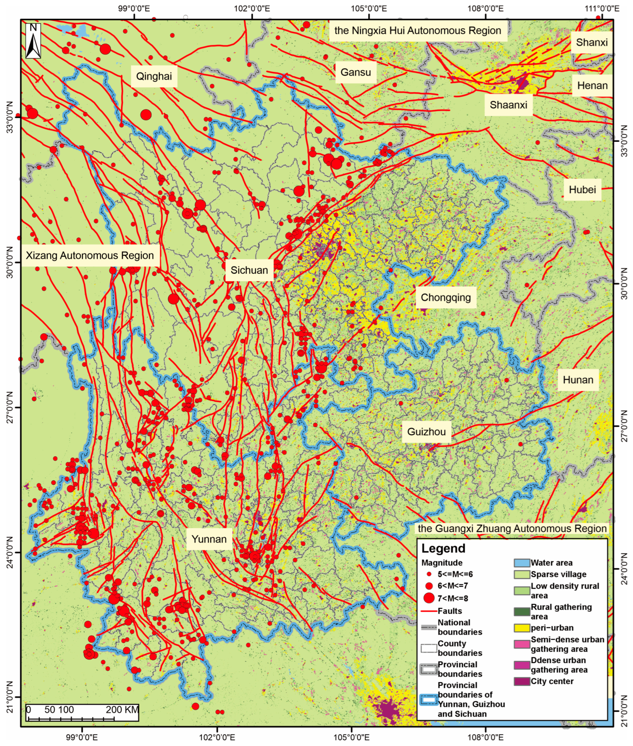
Figure 1. Distribution of settlements and historical earthquakes with a magnitude of M 5.0 or greater in southwestern China.
Applsci 16 06257 g001
Figure 2. Basic geographic information of Yunnan, Guizhou, and Sichuan provinces (partial display).
Applsci 16 06257 g002
Figure 3. Comparison of population grid data from three sources in Weining Yi Autonomous County, Guizhou Province: (a) 2021 population data from the Chinese mobile terminal public service ‘Cube Data Society’; (b) 2020 population data from the European Space Agency (ESA); (c) 2016 population data from the Institute of Earthquake Prediction, China Earthquake Administration (CEA).
Applsci 16 06257 g003
Figure 4. Distribution of PGA with a probability of exceeding 10% over 50 years in Yunnan, Guizhou, and Sichuan.
Applsci 16 06257 g004
Figure 5. Distribution of the residential building inventory by household size in Yunnan, Sichuan, and Guizhou provinces.
Applsci 16 06257 g005
Figure 6. The proportion fan diagram illustrating the distribution of households with various building structures across counties in southwestern China.
Applsci 16 06257 g006
Figure 7. The flowchart illustrates the procedures for data preprocessing and region mapping calculations. Dashed lines indicate correspondence or associative relationships, whereas solid unidirectional arrows denote directional output relationships.
Applsci 16 06257 g007
Figure 8. Seismic intensity zoning in Yunnan, Guizhou, and Sichuan with a PGA probability exceeding 10% over a 50-year period.
Applsci 16 06257 g008
Figure 9. Distribution of population in Yunnan, Guizhou, and Sichuan by 2020.
Applsci 16 06257 g009
Figure 10. The kilometer grid depicting the lethal level in Yunnan, Guizhou, and Sichuan with a PGA probability exceeding 10% over a 50-year period.
Applsci 16 06257 g010
Figure 11. Methodological flowchart depicting the construction of the lethality/injury matrix and its interaction with intensity parameters and human population grids in this study. Dashed-line boxes designate explanations of data types at the equivalent hierarchical level or illustrate processing content as indicated by adjacent black arrows, while solid unidirectional arrows represent directional output relationships.
Applsci 16 06257 g011
Figure 12. The estimated kilometer grid of earthquake fatalities in southwestern China with (a) a 50-year probability of occurrence of 63%; (b) a 50-year probability of occurrence of 10%; (c) a 50-year probability of occurrence of 2%; and (d) a one-year probability of occurrence of 10−4.
Applsci 16 06257 g012
Figure 13. The estimated earthquake fatalities by counties of southwestern China with (a) a 50-year probability of occurrence of 63%; (b) a 50-year probability of occurrence of 10%; (c) a 50-year probability of occurrence of 2%; and (d) a one-year probability of occurrence of 10−4.
Applsci 16 06257 g013
Figure 14. The estimated kilometer grid of earthquake injuries in southwestern China with (a) a 50-year probability of occurrence of 63%; (b) a 50-year probability of occurrence of 10%; (c) a 50-year probability of occurrence of 2%; and (d) a one-year probability of occurrence of 10−4.
Applsci 16 06257 g014
Figure 15. The estimated earthquake injuries by counties of southwestern China with (a) a 50-year probability of occurrence of 63%; (b) a 50-year probability of occurrence of 10%; (c) a 50-year probability of occurrence of 2%; and (d) a one-year probability of occurrence of 10−4.
Applsci 16 06257 g015
Figure 16. The predicted casualties in the districts and counties of Yun Gui Chuan varies with the probability of exceeding PGA.
Applsci 16 06257 g016
Figure 17. Spatial distribution of predicted mortality rates under a 10% GPA exceedance probability in 50 years: (a) districts with mortality rates exceeding 0.0135%; (b) districts with mortality rates below 0.0135%.
Applsci 16 06257 g017
Figure 18. Active tectonic setting of the Yunnan–Guizhou–Sichuan region, China.
Applsci 16 06257 g018
Table 1. Historical earthquakes above M7.0 in southwest China.
ProvinceCounty/CityYearMonthDayMagnitude (M)Longitude
(°)
Latitude
(°)
Depth (km)
YunnanYiliang150014≥7.0103.124.9-
Yongsheng15156177.75100.726.7-
JIianshui-quxi158889≥7.00102.824-
Nidu16527137100.625.2-
Dongchuan-Ziniupo1733827.75103.126.3-
Huaning1789677102.924.2-
Shiping-baoxiu17998277102.423.8-
Songming-yanglin183396810325-
Shiping188712167102.523.7-
Eshan191312217102.524.2-
Dali19253167100.425.7-
Gengma1941516799.423.6-
Lancang19411226799.922.7-
Menghai1950237100.121.7-
Tonghai1970157.8102.724.213
Daguan19745117.1104.128.214
Longling19765297.39924.524
Longling19765297.498.724.621
Gengma19881167.299.5523.1616
Lancang19881167.499.7922.9213
Yuulong1996237100.2227.310
SichuanDetuo1786610≥7.00102.229.4-
Leibo-Mahu12163177103.828.4-
Xichang15363197.5102.228.1-
Mao-diexi1713947103.732-
Kangding1725817101.930-
Kangding1786617.7510229.9-
Luhuo18161287.5100.731.4-
between Xichang and Puge18509127.5102.427.7-
Batang18704117.2599.130-
Daofu-qianning18938297101.530.6-
Shiqu-luoxu18963179832.5-
Daofu19048307101.131-
Luhuo19233247.310131.5-
Mao19338257.5103.431.9-
Litang19485257.3100.529.5-
Kangding19554147.5101.830-
Luhuo1973267.6100.731.311
Songpan19768167.2104.132.615
Pingwu19768237.2104.332.523
Wenchuan20085128103.43114
Lushan2013420710330.313
Jiuzhaigou2017887103.8233.220
Table 2. Comparative evaluation of permanent resident population data (officially reported statistics by the Seventh National Population Census) in the study area against ESA population grid data (2020).
IndexYunnanGuizhouSichuanTotal or Average of Three Provinces
Sample size (number of counties)12988183390
MAE (ten thousand people)4.23.85.14.4
RMSE (ten thousand people)5.75.26.85.9
R20.900.930.920.92
Proportion of counties with relative error ≤ 10%82.1%79.5%84.7%84.7%
Table 3. Comparison of PGA and seismic intensity for class II sites in China [56].
PGA of Class II Sites in China0.04 g ≤ amaxII < 0.09 g0.09 g ≤ amaxII < 0.19 g0.19 g ≤ amaxII < 0.38 g0.38 g ≤ amaxII < 0.75 gamaxII ≥ 0.75 g
Seismic intensityVIVIIVIIIIX≥X
Table 4. Number and proportion of households by building structures in urban areas of Chengdu City, Sichuan, China from the population census.
CountySteel and Steel–Concrete StructureBrick–
Concrete Structure
Brick–Wood StructureVegetation StructureOther StructuresSteel and Steel–Concrete Structure Proportion (%)Brick–
Concrete Structure Proportion (%)
Brick–Wood Structure Proportion (%)Vegetation Structure Proportion (%)Other Structure Proportion (%)
Chengdu509,335397,652105,657499912150.04%39.07%10.38%0.49%0.01%
Jinjiang33,78730,3463234141050.05%44.95%4.79%0.21%0.00%
Qingyang34,14328,2905609221050.02%41.44%8.22%0.32%0.00%
Jinniu46,03632,21013,263508150.03%35.00%14.41%0.55%0.00%
Wuhou42,40829,35812,545436050.04%34.64%14.80%0.51%0.00%
Chenghua48,85339,7708777166150.07%40.76%9.00%0.17%0.00%
Chengdu High-tech Zone38,64233,669481718050.09%43.64%6.24%0.02%0.00%
Long Quanyi38,19926,41811,545189350.03%34.60%15.12%0.25%0.00%
Table 5. Number and proportion of households by building structures in township areas of Chengdu City, Sichuan, China from the population census.
CountySteel and Steel–Concrete StructureBrick–
Concrete Structure
Brick–Wood StructureVegetation StructureOther StructuresSteel and Steel–Concrete Structure Proportion (%)Brick–
Concrete Structure Proportion (%)
Brick–Wood Structure Proportion (%)Vegetation Structure Proportion (%)Other Structure Proportion (%)
Chengdu27,55611,47630959716265.01%27.07%7.30%0.23%0.38%
Jinjiang00000
Qingyang00000
Jinniu00000
Wuhou00000
Chenghua00000
Chengdu High-tech Zone00000
Longquanyi District414415324847.42%47.54%3.67%0.46%0.92%
Qing baijiang707741343647.42%49.70%2.28%0.20%0.40%
Xindu205222890089.65%9.96%0.39%0.00%0.00%
Wenjiang444369340152.36%43.51%4.01%0.00%0.12%
Shuangliu35349141084.65%11.75%3.36%0.24%0.00%
Pidu569347782057.13%34.84%7.83%0.20%0.00%
Xinjin379200683258.13%30.67%10.43%0.46%0.31%
Jintang95652675147604676.56%21.41%1.18%0.48%0.37%
Dayi5718269949904363.82%30.13%5.57%0.00%0.48%
Pujiang276981332481270.53%20.71%8.25%0.20%0.31%
Tianfu New District00000
Eastern New District of Chengdu84131195834.01%53.04%7.69%2.02%3.24%
Du Jiangyan9186803122347.94%35.51%16.29%0.10%0.16%
Pengzhou11317991271154.93%38.81%6.17%0.05%0.05%
Qionglai88257258611043.00%27.89%28.57%0.05%0.49%
Chongzhou123741677221150.74%17.06%31.67%0.08%0.45%
Jianyang3343424051145.63%46.72%5.46%0.68%1.50%
Table 6. Number and proportion of households by building structures in rural areas of Chengdu City, Sichuan, China from the population census.
CountySteel and Steel–Concrete StructureBrick–
Concrete Structure
Brick–Wood StructureVegetation StructureOther StructuresSteel and Steel–Concrete Structure
Proportion (%)
Brick–
Concrete Structure Proportion (%)
Brick–Wood Structure Proportion (%)Vegetation Structure Proportion (%)Other Structure Proportion (%)
Chengdu50,04161,83730,216149495934.62%42.78%20.90%1.03%0.66%
Jinjiang00000
Qingyang00000
Jinniu00000
Wuhou00000
Chenghua00000
Chengdu High-tech Zone43152231419.28%68.16%10.31%0.45%1.79%
Longquanyi District3201764112211814.32%78.93%5.01%0.94%0.81%
Qingbaijiang10952926417301824.41%65.23%9.30%0.67%0.40%
Xindu24256387775153125.17%66.30%8.05%0.16%0.32%
Wenjiang3429228470134353.08%35.36%10.85%0.05%0.67%
Shuangliu75923162685105166.02%27.50%5.96%0.09%0.44%
Pidu39256095901354335.69%55.41%8.19%0.32%0.39%
Xinjin1469130975982041.21%36.72%21.29%0.22%0.56%
Jintang33558683100760720624.21%62.66%7.27%4.38%1.49%
Dayi328012433891205538.64%14.64%45.84%0.24%0.65%
Pujiang165310431806214236.21%22.85%39.56%0.46%0.92%
Tianfu New District301434446361211641.68%47.63%8.80%1.67%0.22%
Eastern New District of Chengdu108338518512364917.84%63.44%14.02%3.89%0.81%
Du Jiangyan316834751929143836.73%40.29%22.37%0.16%0.44%
Pengzhou345267333376105425.34%49.42%24.78%0.07%0.40%
Qionglai188119965628239419.55%20.74%58.49%0.24%0.98%
Chongzhou340721354991174732.15%20.15%47.10%0.16%0.44%
Jianyang54505155172830213042.69%40.38%13.54%2.37%1.02%
Table 7. Urban/rural zoning codes of China (CNBS).
Area ClassificationThe Main Urban AreaThe Urban–Rural Integration ZoneThe Town Center AreaThe Town–Rural Integration ZoneSpecial Township AreaThe Rural Central AreaVillage
Urban/Rural Zoning Codes111112121122123210220
Table 8. Range and influencing factors of lethal levels in buildings [18,52] (Nie et al. 2020, 2021).
Building Structure TypeInfluence FactorsLethal Level
Building TypeSecondary Classification
Steel structure Construction measures, foundation type, construction time, and purpose0.05–0.15
Frame structureFaConstruction measures, foundation type, construction time, height0.1–0.3
Fb
Timber structureWaConstruction measures, foundation type, construction time, structural style0.2–0.4
Wb
Brick-concrete structureBa (Fortified)Construction measures, foundation type, construction time, purpose, height0.25–0.7
Bb (Non-Fortified)
Brick-wood structureMaConstruction measures, foundation type, construction time, structural style0.6–0.9
Mb
civil structured Construction measures, foundation type, construction time, building materials0.7–0.95
Stone (wood) structure Wall type, foundation type, construction time, building materials0.55–0.9
Adobe structure Wall type, foundation type, construction time, building materials0.85–1.0
Table 9. Validation of this model using certain historical earthquakes in China [36,37].
Location of EarthquakeTime
(Year–Month–Day)
MagnitudeLethal GradeActual CasualtyCalculated CasualtyErrorPre-Estimated Casualty
Lancang Gengma, Yunnan6 November 19887.630%7487834.68%700–850
Ning’er, Yunnan3 June 20076.470%33.8729.00%0–5
Yushu, Qinghai14 April 20107.10%26982197−18.57%1800–3000
Lushan, Sichuan20 April 20137.080%196165−15.82%150–200
Min County-Zhang, Gansu 22 July 20136.640%95 + 598−2.00%85–120
Ludian, Yunnan3 August 20146.510%617596−3.40%550–700
Jinggu, Yunnan 7 October 20146.680%13.07precise 0–5
Jiuzhaigou, Sichuan8 August 20177.060%2925.9810.41%10–40
Table 10. List of counties and corresponding emergency response levels predicted for seismic deaths exceeding 10% probability over a 50-year period in southwestern China.
Predicted Death TollEmergency Response LevelCorresponding County Counts
2000~3000I1 (Xichang City)
1000~1999I1 (Lancang County)
500~999I3 (Xundian/Songming/Dongchuan)
100~499II44
10~99III159
1~10IV192
Table 11. List of counties corresponding to the predicted number of seismic injuries with a PGA probability exceeding 10% over a 50-year period in southwestern China.
Predicted Number of InjuredCorresponding County Counts
10,000~20,0001 (Xichang City)
5000~99997 (Lancang/Tengchong/Longyang/Xundian/Songming/Yiliang//Panlong)
2000~499947
1000~199926
500~99926
100~49965
0~100228
Table 12. List of counties and corresponding emergency response levels predicted for seismic deaths exceeding 63% probability over a 50-year period in southwestern China.
Predicted Death TollEmergency Response LevelCorresponding County Counts
500~I0
100~499II0
10~99III16
1~10IV102
Table 13. List of counties and corresponding emergency response levels predicted for seismic deaths exceeding 2% probability over a 50-year period in southwestern China.
Predicted Death TollEmergency Response LevelCorresponding County Counts
500~I100
100~499II97
10~99III176
0~10IV27
Table 14. List of counties and corresponding emergency response levels predicted for seismic deaths exceeding 10−4 probability over a one-year period in southwestern China.
Predicted Death TollEmergency Response LevelCorresponding County Counts
500~I164
100~499II66
10~99III143
0~10IV27
Table 15. Statistical analysis of mortality rate changes across different GPA exceedance probability intervals in 400 districts and counties.
Statistical IndicatorThe Probability of Exceeding the GPA Exhibits a Variation Spanning from 0.01% Within a One-Year Period to 2% Over a 50-Year PeriodThe Exceedance Probability of Generalized Pareto Distribution (GPA Exhibits a Variation Range Spanning from 2% Over a 50-Year Period to 10% Over a 50-Year PeriodThe Exceedance Probability of the GPA Exhibits a Variation Spanning from 10% Over a 50-Year Period to 63% Over a 50-Year Period
count400400400
mean−0.293573−0.91−0.97
std0.3617680.030.10
min−0.932491−1.00−1.00
25%−0.679755−0.93−1.00
50%−0.004870−0.90−0.99
75%0.000000−0.88−0.97
max0.000000−0.860.25
Table 16. Sensitivity differences across different PGA exceedance probability intervals.
PGA Exceedance Probability IntervalsAverage Rate of ChangeMedian Change RateSensitivity Characteristics
0.01% in 1 year → 2% over 50 years−29.4%−0.5%The lowest sensitivity was observed, with no changes in nearly half of the districts and counties.
2% over 50 years → 10% over 50 years−90.5%−90.0%Highly sensitive, with a sharp decline in mortality
10% over 50 years → 63% over 50 years−96.8%−99.4%Extremely sensitive, with near-zero mortality rates
Table 17. Stability ratio of predicted death rate intervals by district/county of Yun Gui Chuan.
Death Toll Range by District and CountyStability RatioStability Characteristic
<5096.5%extremely high stability
50–20072.2%Higher stability
200–100013.6%Low stability
>1000~5–6%Almost no stability
Table 18. Comparative analysis of the sensitivity of typical spatial data transformation methods.
Comparison DimensionVoronoi PolygonKrychkin MethodInverse Distance Weighting Method (IDW)Natural Neighborhood Method
parameter dependencyHigh (uniformity of dependency point distribution) <block index = “1396”>Highly elevated (requires fitting a spatial autocorrelation model)Medium (dependence distance attenuation parameter)Medium (depending on the topological relationship of adjacent points)
Parameter sensitivityLow (requires only point coordinates and weights)High (semi-variance function parameters have a significant impact)Medium (Power index selection affects results)Medium (neighborhood area weight calculation sensitivity)
Boundary effectHigh (clear boundary, significantly influenced by adjacent points)Low (smooth boundary for continuous surfaces)Medium (with “bull eye effect”)Low (Smooth boundary transition)
Dynamic update efficiencyHigh (adjust adjacent cells locally) <block index = “1396”>Low (global model recalculation)Medium (requires recalculating weights)Medium (reconstruction using dependent triangular network)
Disclaimer/Publisher’s Note: The statements, opinions and data contained in all publications are solely those of the individual author(s) and contributor(s) and not of MDPI and/or the editor(s). MDPI and/or the editor(s) disclaim responsibility for any injury to people or property resulting from any ideas, methods, instructions or products referred to in the content.