Reverse Automaton Modified Map Dimension Reduction for Stable Assisted Driving of Smart Trackless Rubber-Tired Vehicles

Abstract

Trackless rubber-tired vehicles are the important auxiliary transportation equipment in coal mines. The main difficulty of their unmanned driving is that the underground environment information is complex but the onboard computing resources for perception and measurement are limited. To solve this conflict, this paper establishes a lightweight map dimension reduction framework to assist in path planning. Firstly, motivated by the idea of image convolution, the framework using the simplicity kernel is proposed for the high-resolution grid maps, which can reduce planning time while retaining the useful map information. Secondly, the reverse automata based on the greedy strategy are designed to get suitable machine-selected key points, which can solve the problem that some self-selected key points become impassable because of the dimension reduction. Moreover, a Bezier smoothing method based on slope interpolation is presented to avoid the collision between the smooth path and obstacle grid caused by the small number of path points planned on the reduced-dimension map. Finally, comparison experiments and downhole map experiment are carried out and discussed. The results show that using the proposed method to assist path planning can reduce time by 99.77% and reduce the number of redundant path points by 79.60%, and using the improved smoothing method from the framework can avoid collision risks caused by fewer path points.

1. Introduction

Trackless rubber-tired vehicles (TRTVs) are the new transportation in the development of mine modernization for auxiliary transportation [1]. Their intelligence can free workers from high risk in the downhole. The latest intelligent TRTVs usually first plan the drivable routes offline, and then use autonomous obstacle avoidance algorithms to achieve autonomous decision-making during operation [2]. In the existing research, the real-time control [3,4] and decision-making that require a large amount of computing resources and power supply are widely studied. Nevertheless, due to the limitations of confined space and large amounts of flammable gas and dust, the TRTVs must be equipped with intrinsically safe or explosion-proof memory, sensors, and low-voltage processing units in the mine [5]. The system security and transportation efficiency, when only improving decision-making and control performance of TRTVs, are constrained by the hardware performance in the mine [6]. In addition, in special transportation work, the route of TRTVs often undergoes temporary changes due to semi-permanent tunnels and material accumulation. TRTVs generally need to quickly find a drivable path that can reach the task destination [7]. Therefore, considering the impact of planning on mining tasks and studying how to obtain a safe and smooth path in a short period would be an ideal strategy to retain more computing and memory resources for the real-time unmanned driving systems (i.e., the perception system, the decision-making and control system, etc.) in coal mines. This may further improve the safety and efficiency of transportation in complex environments such as underground.

In recent decades, scholars [8,9] have proposed some improved path planning algorithms for intelligent vehicles to address issues of low planning efficiency and high energy consumption in narrow or complex scenes. These strategies are commonly based on reinforcement learning [10], rapidly exploring random tree [11], swarm intelligence optimization algorithms [12,13], deep neural network [14,15], etc., which focus on the improvement of algorithms, but ignore the important impact of the environment map models [16]. The roof, floor and surrounding rock of the underground tunnel in the coal mines are rugged because of the long-term elastic–plastic deformation of argillaceous soft rock on deep confined space. The grid map [17] as the general map model is suitable for the coal mine to build the environment map. This model is widely used for various complex realistic conditions, and can define the obstacle information by setting grid values [18]. It also has many advantages, e.g., mature supporting technologies, high reliability, strong universality, etc. With the development of artificial intelligence technologies, the map models not only provide data for path planning, but also contain more information for intelligent decision-making, including the types of obstacles, the characteristics of the environment [19] and the location of TRTVs [20], etc., which are redundant and useless for path planning and increase the burden on the onboard computing cells and memory on TRTVs.

Currently, map downsampling is the primary method for reducing map scale in ground vehicle navigation. Typical solutions include environmental resampling and point-cloud-based dimensionality-reduction algorithms, such as Principal Component Analysis (PCA) and Linear Discriminant Analysis (LDA) [21]. However, these conventional downsampling methods suffer from evident limitations in underground mine scenarios. They require additional sensor data preprocessing, which increases sensor workload and overall computing latency. In addition, the traditional PCA or LDA point-cloud downsampling easily distorts local spatial features and erodes critical obstacle boundary information, which is intolerable for high-risk underground driving tasks. Most importantly, these methods cannot fundamentally reduce the resource occupancy of grid map data or adapt to the discrete grid characteristics required for mine path planning. Thus these solutions increase the workload and computing time of sensors, and cannot fundamentally alleviate the burden of power, computing cells and memory. In recent years, the image processing technology based on deep learning has developed rapidly. Inspired by its working idea on images, it is a possible alternative to reduce the amount of information irrelevant to path planning in the high-resolution static environment map model, so as to shorten the path planning time.

Although the map model processing method can improve the path planning efficiency of TRTVs, it may also bring security problems, especially collisions, to transportation routes [22]. The collision-free paths of TRTVs in mines are preferably planned far enough away from the obstacles for safety considerations. In fact, the conventional path planning methods [23,24] (e.g., A*, D*, etc.) just plan the path to bypass the impassable grid, which means that the planned passable path is alongside the edge of obstacles. Nevertheless, the working environment of TRTVs for mining often has many protrusions and other static objects [25], e.g., bolts, puddles, gangue in the coal mine environment. When the TRTV passes around these obstacles, the risk of TRTV scratching and colliding with obstacles may increase due to the mine roof falling off, instability of the tunnel floor, etc. The existing solutions are to use the envelope body or increase the vehicle volume in path planning to avoid corner collisions [26], but the underground roadway is long and narrow, and the use of the envelope body may greatly lead to planning failure.

To solve the above issues, in our previous work, a map dimension reduction framework for high-resolution 0–1 grid maps of TRTVs for planning was proposed, motivated by the idea of image convolution, with the goal of minimizing the impact of redundant information on planning, enhancing planning efficiency, and conserving resources for online perception and decision-making [27]. The proposed framework serves as a potential substitute for reducing the amount of information unrelated to path planning in the high-resolution static environment map model. In our recent research, we found that the early versions did not fully meet the path planning requirements of mining [28]. The basic high-resolution static grid map carried in TRTVs may also be a numerical map [18] used to define obstacle information rather than the 0–1 grid maps. In addition, despite planning a collision-free path on the dimensionality-reduction map, TRTVs face a safety risk from collisions with obstacle corners when traversing the smooth path [29], particularly in sections requiring continuous turns. Therefore, the map dimensionality-reduction framework was extended to numerical grid maps in this paper. The reverse automata and improved Bezier smoothing method were also proposed to compensate for the bugs that may be encountered when using dimensionality-reduction frameworks to assist path planning. The former is inspired by cellular automata, which can find passable grids around key grids that cannot be processed after map dimensionality reduction. The latter can reduce collisions between TRTV paths and obstacle corners caused by path planning algorithms. The dimensionality-reduction methods of simplicity kernel, the path safety, and the characteristics of dimensionality-reduction frameworks, etc., are discussed, using maps with typical downhole characteristics, e.g., meandering, dense obstacles, and small exits.

The main contributions of this paper are as follows.

• The map dimension reduction framework (MDRF) is proposed to assist in path planning. It is suitable for the working conditions of vehicles with limited onboard sensor performance and computing resources.
• The greedy strategy-based reverse automaton (GRA) is proposed to be applied to 0–1 and numerical grid maps, which can find passable grids and fix the issue of multiple machine-selected key points.
• A slope interpolation-based Bezier curve smoothing method (SIBS) is proposed to reduce the collision risk between smooth paths and obstacles caused by fewer path points planned on the maps using the MDRF.

The remainder of this paper is organized as follows. Section 2 briefly introduces the fundamental theories and preliminary techniques adopted in our work. Section 3 elaborates the proposed framework and corresponding improvement strategies. In Section 4, comparative experiments and comprehensive discussions are conducted to validate the superiority and feasibility of the proposed method. Finally, the conclusions and future prospects of this study are summarized.

2. Preliminaries

2.1. Convolution Principle

Deep learning [30,31] as a common image processing method has made great progress in the past decades. Its idea is to use convolutional neural networks to autonomously obtain and retain the feature information in images, wherein the convolution kernel and convolution processing play a crucial role. The convolution kernel can perform traversal convolution on the current image to reduce the image dimension and enhance the feature information of the current image. The principle of convolution and the convolution kernel are shown in Figure 1.

As can be seen from Figure 1, its working principle is to use the convolution kernel to traverse the two-dimensional matrix of the image. Starting from area 1, the convolution kernel and local image information are multiplied and summed one by one, and then convolution is performed on area 2 until the whole image processing is completed. The result is to output the convolved image. When the image is convolved, it is assumed that the original image dimension is $n\times m$, and the image matrix dimension after convolution is $(n-2)\times (m-2)$. By increasing the convolution depth, the matrix dimension can be reduced to the ideal level. This process can effectively reduce the dimension of the image, and retain different effective features of the image according to different convolution types. The grid map is also a matrix that contains fewer data features than images, and the reciprocating full coverage dimensionality-reduction type like convolution is suitable for map dimensionality reduction due to the physical significance (e.g., position and geodetic transformation, etc.) of grids. Therefore, inspired by this idea, the simplicity kernel is defined and MDRF is designed to reduce the dimension of the grid map.

2.2. Cellular Automata

Cellular automata (CA) [32] is a general term for a class of grid dynamic models. It was proposed by Von Neumann and used to simulate the phenomenon of machine learning. The model does not contain the specific physical formulas and functions, but consists of cells, cell states, evolution rules, etc. It has the capability to simulate the spatiotemporal evolution of complex dynamic systems. It can be expressed as:

$$A=(L_d,S,N,f),$$

(1)

where A represents a cellular automaton system. $L_d$ is the cell space, representing the dimension of the cell space. S represents the state of the cell, which is finite and discrete. N is the state set of cells in the neighborhood. f represents the evolution rule.

Stephen Wolfram’s research [33] has played a decisive role in promoting the development of CA. He introduced the theory of dynamics and the simplified structure of CA. In his theory, CA has the following five basic characteristics:

• Cells are distributed in the discrete cell space divided according to certain rules.
• The evolution of the system is carried out step by step with equal intervals of time, and the time variable is taken as the time point with equal step size.
• Each cell has a definite state, and the state of the cell can only take a finite number of discrete values.
• The state value of cell evolution at the next time is determined by the determined transformation rules.
• The transformation rule of each cell is only determined by the cell state in the local domain.

Due to the highly efficient evolutionary and discrete characteristics of CA, some scholars have applied it to robotics [34,35]. As shown in the existing literature, path planning based on CA requires knowing the grid information, the evolutionary starting point, the evolutionary range, the evolutionary rules and the evolutionary target points. However, in practical engineering applications of TRTVs, the last three conditions are usually unknown, so some improvements need to be proposed.

2.3. Bezier Curve

The Bezier curve was proposed by Paul de Casteljau [36], and then widely used in automobile appearance design by Pierre Bezier [37]. In theory, a Bezier curve can represent all lines and curves according to the number and position of control points. Taking advantage of its good continuity and the characteristics that just the head and tail control points are on the curve, it becomes advantageous to smooth the path of robots [38,39]. The Bezier curve is described by Equation (2):

$$P\left(u\right)={\displaystyle \sum _{i=0}^n}{B}_i^n\left(u\right)P_i,0\le u\le 1,$$

(2)

where u is the normalized time variable. $P_i$ is the i-th control point. $B_i^n\left(u\right)$ is the Bezier basis function as follows:

$$B_i^n\left(u\right)=\left[\begin{array}{c}n\\ i\end{array}\right]u^i{(i-u)}^{n-i},i=0,1,\cdots ,n.$$

(3)

It can be seen from Equation (2) that each point on the Bezier curve is the weighted sum of these control points, and the curve basis function is the weight value. For example, on the Bezier curves of third and fifth orders in Figure 2, it can be observed that the Bezier curve is completely contained in a polygonal convex hull composed of a series of control points, and just includes the head and tail control points on the curve.

3. The Map Dimension Reduction Framework

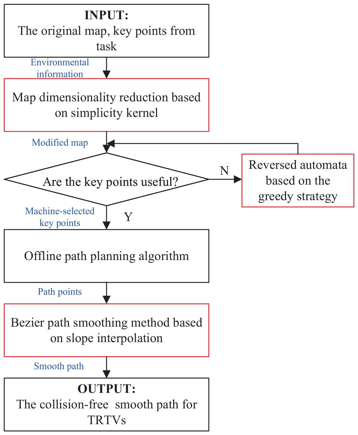
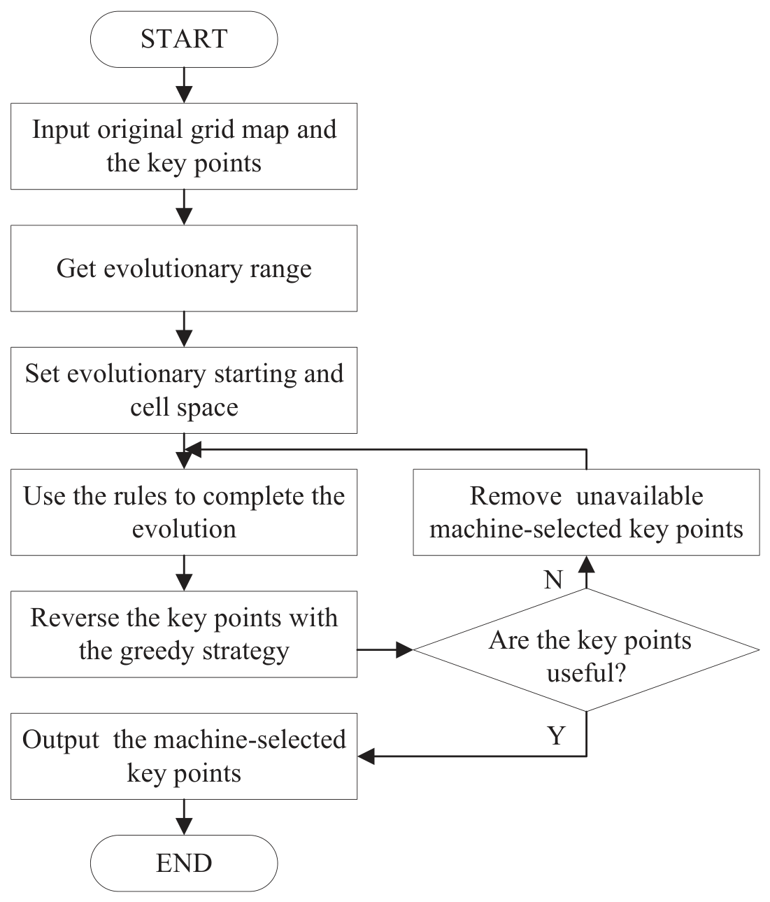
Figure 3 displays the flow chart of the proposed MDRF. First of all, MDRF, the major contribution, is used to rapidly reduce the dimension of the existing high-resolution grid map, and retain the effective feature information. Secondly, it is concurrently evaluated whether the dimension reduction has rendered the key points on the modified map unavailable. If the key points (start point, endpoint, and other important nodes) are unavailable, GRA is used to obtain the appropriate machine-selected points to participate in the path planning. After path planning, SIBS calculates a collision-free smooth path. It can modify the smooth path by incorporating a few smooth control points to prevent collisions with the corners of obstacles.

3.1. Map Dimension Reduction Framework Based on Simplicity Kernel

In order to shorten the path planning time and reduce computing power consumption, most of the current relevant strategies are to improve the path planning algorithms. Although such methods have achieved good results, they are still challenged in the face of increasingly refined environmental map models. Motivated by the idea of convolution and the convolution kernel applied in image processing, it is theoretically feasible to reduce the dimension of the environmental map model, which is also one aspect of the matrix, to shorten the path planning time. Therefore, the goal of MDRF is to use reasonable strategies to zoom in on the basic grid map and retain the environmental characteristics and physical properties of grids before path planning.

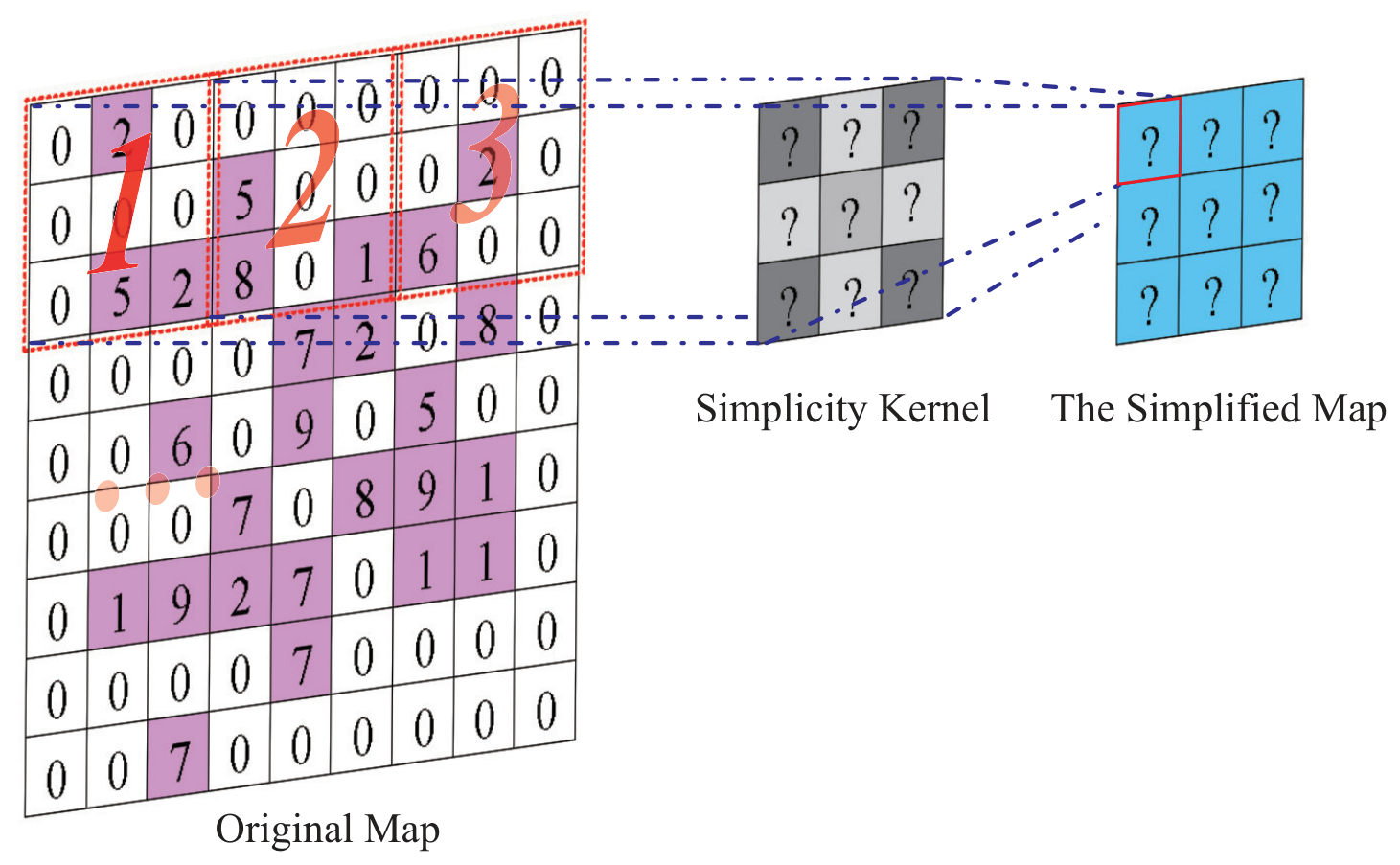
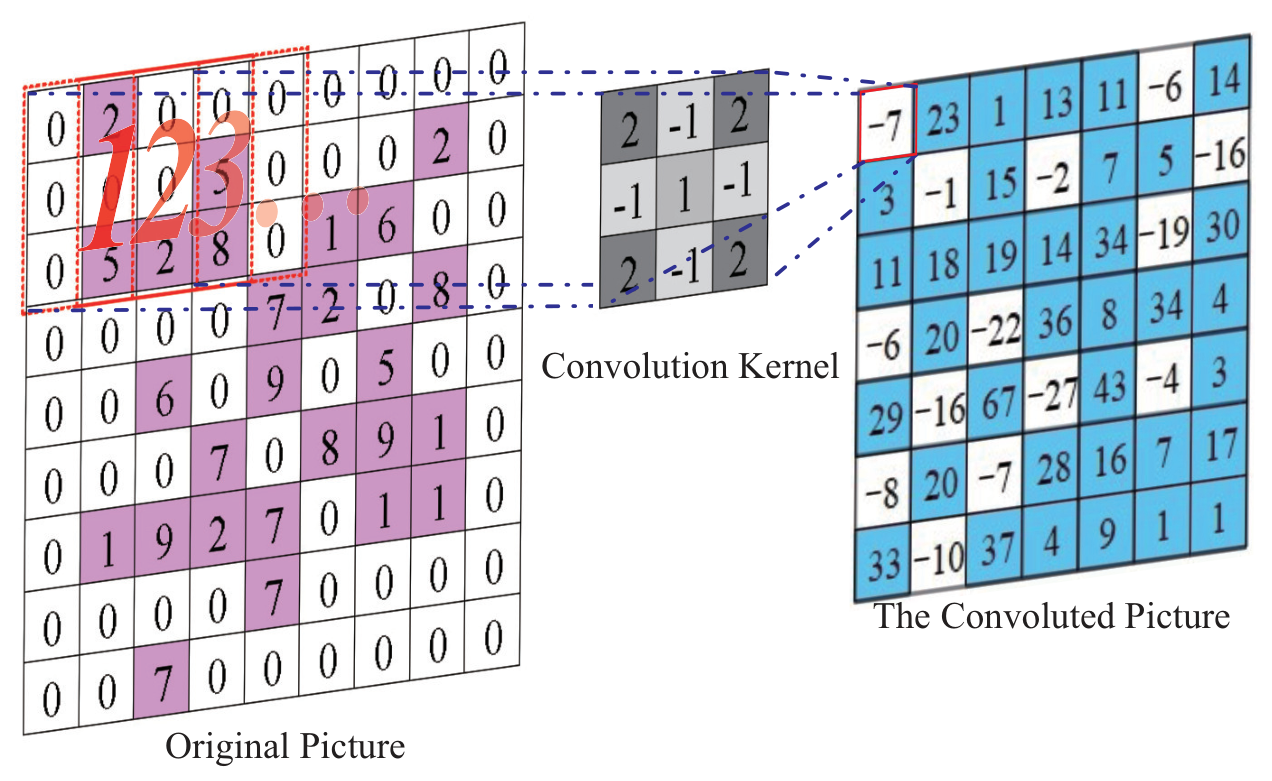
The principle of the simplicity kernel is shown in Figure 4. The simplicity kernel traverses the entire grid map from the top-left corner to implement map dimensionality reduction. Its core distinction from the standard convolution principle illustrated in Figure 1 lies in the sampling mode of the original grid data. After completing the downsampling operation for one group of map grids, the kernel selects the nearest non-overlapping grid set for subsequent dimensionality reduction. This mechanism enables proportional scaling of the overall grid map size while completely preserving the obstacle distribution information of each local region.

In the previous work [27], we adopted the method of preserving obstacle grids to preserve features of the 0–1 grid map when reducing the dimension. The simplicity kernel and its dimension reduction process are described by

$$g(i,j)=\max \left(\max \left(G(i:(i-s_1+1),j:(j-s_2+1))\right)\right),$$

(4)

where $g(i,j)$ is the maximal feature extraction function to obtain the reduced dimension map data. $G_{i:(i-s_1+1),j:(j-s_2+1)}$ represents neighborhood grid data in row i and column j of the grid on the basic map. $s_1$ and $s_2$ are the row and column size of the simplicity kernel, respectively.

In this paper, the dimensionality-reduction framework is extended to numerical maps. Numerical maps not only contain obstacle information, but also each grid has different values and meanings; thus, Equation (5) is first used to normalize, which normalizes each grid value to $[0,255]$.

$$GN(i,j)={\displaystyle \frac{(255-0)\times (M_{i,j}-M_{\min })}{(M_{\max }-M_{\min })+0}},$$

(5)

where $GN(i,j)$ represents the normalized function for the grid data in row i and column j. $M_{i,j}$ is the value of the grid in row i and column j. $M_{\max }$ is the maximal value of the numerical map, and $M_{\min }$ is the minimum. The normalized map uses the simplicity kernel as shown in Equation (6) for dimension reduction.

$$g(i,j)={\displaystyle \frac{1}{s_1\times s_2}}\sum G(i:(i-s_1+1),j:(j-s_2+1)).$$

(6)

3.2. Reverse Automata Based on the Greedy Strategy

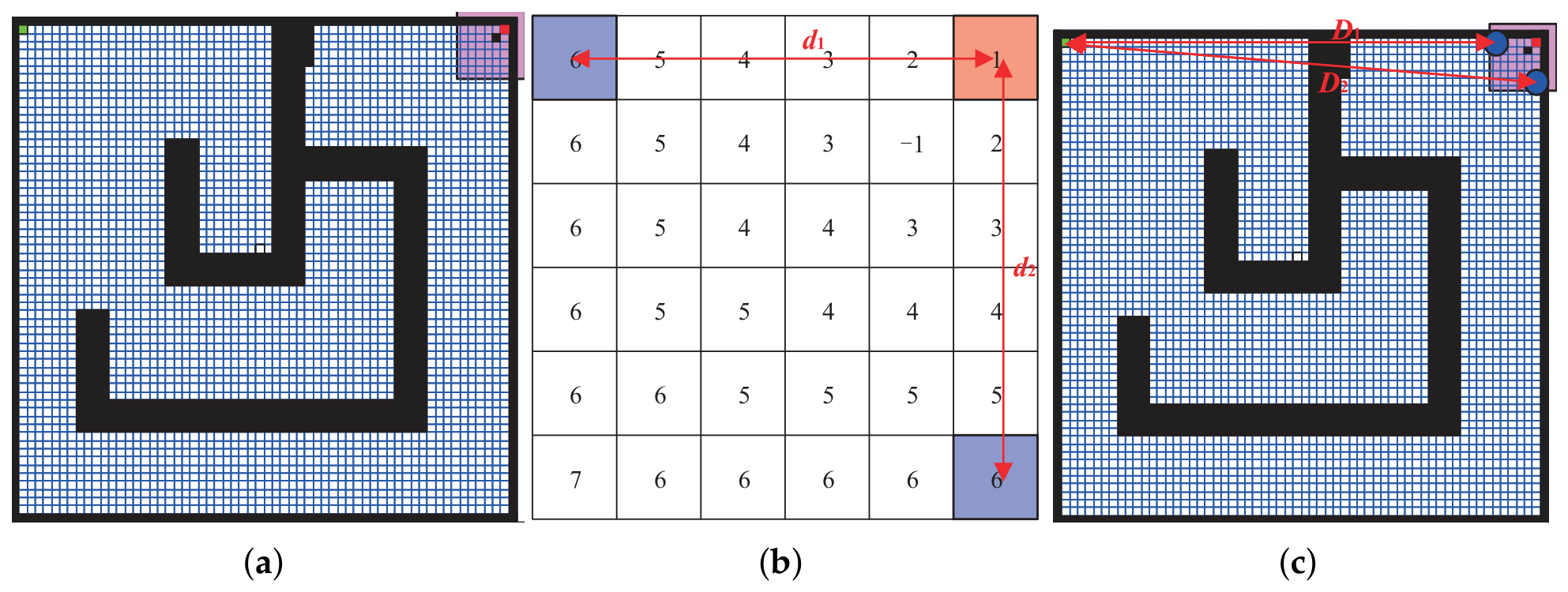
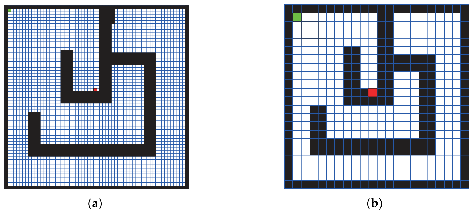
TRTVs need to determine the key-point (starting and end points of the path planning) according to the current position of the vehicle and the destination when assigned a task. However, after map dimension reduction by MDRF, these key points may be determined as impassable grids, resulting in failure of planning, as shown in Figure 5. The green cell is the current position of the vehicle, and the red cell is the position of the task. It can be observed that the red point is close to the edge of the obstacle. After the map dimension reduction, the location of the endpoint is judged to be impassable.

To solve this problem, GRA inspired by the principle of CA is proposed and its flow chart is shown in Figure 6. It can be used to obtain the machine-selected point when the key point is useless for planning after dimension reduction. The cell state, the evolutionary starting point, the evolutionary range, the evolutionary rules, and the evolutionary target points are five important parts of GRA, where the cell state can be obtained according to the grid information, i.e., the grids of the dimension-reduced map are served as the cells, and the invalid key point is set as the evolutionary starting point. The evolutionary range, the evolutionary rules, and the evolutionary target points need to be designed according to the grid maps’ characteristics.

To facilitate the final remapping of the path points onto the high-resolution map and ensure the integrity of the path, the evolutionary range needs to be as small as possible, but not smaller than the dimensionality-reduction size. The evolutionary range of GRA is selected according to the dimension reduction range corresponding to the simplicity kernel and the orientation of the key points on the whole map. The evolutionary range of GRA is selected based on the dimensionality-reduction range corresponding to simple kernels and the direction of key points on the entire map. It can be divided into nine cases exampled in Figure 7 using the 3 × 3 simplicity kernel.

The evolutionary rules and the evolutionary target points for the 0–1 grid map are designed as follows. Rule 1: the impassable grids are set as $-1$, and the evolutionary starting point (unavailable key point) is set as 1. Rule 2: the simplicity kernel size is set as a unit, and the neighborhood range surrounding the key point is taken. Rule 3: the evolution is started from the starting point. When the value of the neighborhood grid is less than the value of the center grid, the value of the neighborhood grid is increased by 1. Otherwise, the neighbor grid is not evolved. Rule 4: when the evolution is completed, the cell that is farthest from the evolutionary starting point in the evolution range with the minimal value is recorded. Rule 5: the cells with decreasing values are deduced backward from the minimal cell, and the shortest distance cell is reserved as the evolutionary target point (machine-selected point) by the greedy strategy and Euclidean distance. After a large number of experiments, some special cases are appeared as shown in Figure 8. It can be observed from Figure 8a that the endpoint is at the corner, which is the impassable grid after dimension reduction. After evolution by GRA, the evolutionary result can be encountered as shown in Figure 8b. It can be seen that two candidate key points with the shortest distancex to the endpoint appear, i.e., $d_1=d_2$. In response to this situation, Rule 6 is presented, i.e., the greedy strategy is used to calculate the Euclidean distance between these two candidate key points and another key point (i.e., the starting point in this case), and the candidate key point with the shortest Euclidean distance is selected as the final machine-selected point. As shown in Figure 8c, the Euclidean distance between the candidate key point in the upper-left corner of the evolutionary range and another key point is less than the Euclidean distance between the candidate key point in the lower-right corner of the evolutionary range and the starting point, i.e., $D_1<D_2$, so the candidate key point in the upper-left corner is selected as the final machine-selected point. The newly added rule is as follows.

Rule 6: if the evolutionary target points are still not unique after Rule 5, the Euclidean distance between these target points and another key point is calculated. The greedy method reserves the shortest evolutionary target point as the machine-selected point.

The elements of a numerical grid map are different from those of the 0–1 grid map. Therefore, the CA based on gray values proposed by Li et al. [40] is adopted to design the evolutionary rules of the numerical grid map and generate evolutionary target points. This CA defines the gray value $G_d^t(x,y)$ to reflect the continuous change of cell $(x,y)$ state, and is used to calculate the mutual evolution process of cities and villages. In this model, the development degree (i.e., gray value) increases in direct proportion to the development probability, and the total constraint coefficient value is given as follows.

$$\Delta G_d^t(x,y)=P_d^t(x,y)\times {\mathrm{CONS}}_d^t(x,y),$$

(7)

where the development probability is calculated by the conventional CA as follows.

$$P_d^t(x,y)=f(S{(x,y)}^t,N).$$

(8)

The development degree and the cell state of the next moment are calculated iteratively using (Equations (9) and (10)).

$$G_d^{t+1}(x,y)=G_d^{t+1}(x,y)+\Delta G_d^t(x,y).$$

(9)

$$S_d^{t+1}=\left\{\begin{array}{cc}\mathrm{developing}\hfill & \hfill G_d^{t+1}=1\\ S_d^t\hfill & \hfill G_d^{t+1}=0\\ \mathrm{partial}-\mathrm{developing}\hfill & \hfill \mathrm{otherwise}\end{array}\right..$$

(10)

Using its evolution principle for reference, the evolutionary rules of the GRA are designed to extend to numerical maps. Rules 1 and 3 are modified as follows, and the other four rules remain unchanged.

Rule 1: the impassable grids are set as $-1$, and the evolutionary starting point (unavailable key point) is set as 1. The values of other grids are normalized to the interval $[0,1]$ according to Equation (11).

$$GN(i,j)={\displaystyle \frac{(1-0)\times (M_{i,j}-M_{\min })}{(M_{\max }-M_{\min })+0}}.$$

(11)

Rule 3: the evolution is started from the starting point and evolves according to (Equations (7)–(10)).

3.3. Bezier Curve Smoothing Method Based on Slope Interpolation

Although the collision-free path can be planned on the dimension reduction map, the number of path control points obtained on the map used MDRF is less than the ones obtained on the basic map. As a result, the collision between the path and the edge of the obstacle may happen when calculating the smooth path, which has a collision safety risk when the TRTV is actually moving.

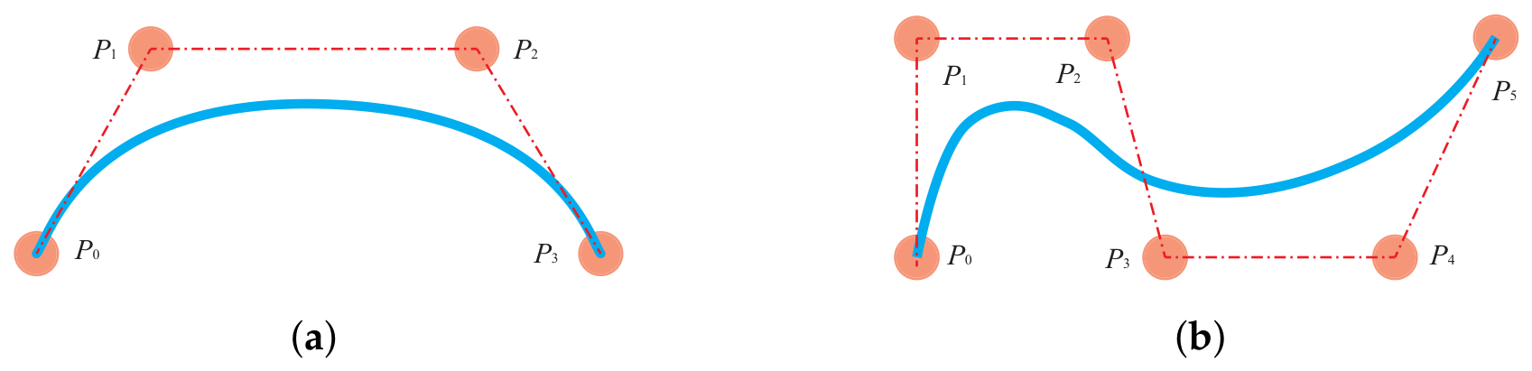
To solve this issue, SIBS is proposed based on the commonly used Bezier curve. When the slope between the path point and the other two path points on both sides is equal, the path point is maintained. Otherwise, the path point is defined as the slope distortion point, and two control points are inserted on both sides of the slope distortion point according to Equation (12) to achieve a smooth path to avoid obstacles:   

$$\begin{array}{cc}\hfill p_1\left(i\right)=& \left[\begin{array}{c}{P}_x^{\prime }(i-1)+\lceil {\displaystyle \frac{P_x^{\prime }\left(i\right)-P_x^{\prime }(i-1)}{2}}\rceil \\ P_y^{\prime }(i-1)+\lceil {\displaystyle \frac{P_y^{\prime }\left(i\right)-P_y^{\prime }(i-1)}{2}}\rceil \end{array}\right]\hfill \\ \hfill p_2\left(i\right)=& \left[\begin{array}{c}{P}_x^{\prime }\left(i\right)+\lceil {\displaystyle \frac{P_x^{\prime }(i+1)-P_x^{\prime }\left(i\right)}{2}}\rceil \\ P_y^{\prime }\left(i\right)+\lceil {\displaystyle \frac{P_y^{\prime }(i+1)-P_y^{\prime }\left(i\right)}{2}}\rceil \end{array}\right]\hfill \end{array},$$

(12)

where $P_x^{\prime }\left(i\right)$ and $P_y^{\prime }\left(i\right)$ are the coordinates of the $i\mathrm{th}$ control point. $p_1\left(i\right)$ and $p_2\left(i\right)$ represent the interpolated control points at both sides of the $i\mathrm{th}$ control point (slope mutation point). $\lceil \ast \rceil$ indicates the rounding-up function.

Its pseudo-code is shown in Algorithm 1, where N represents the number of path points after the path planning, $k_1$ and $k_2$ represent the slope of the lines connected by the $i\mathrm{th}$ path point.

Algorithm 1 The pseudo-code of SIBS

INPUT:  The planned path points including planned, starting and end point. OUTPUT:  The smooth path.   1:  FOR $i=2:N$ do   2:      $k_1=(P_y^{\prime }\left(i\right)-P_y^{\prime }(i-1))/(P_x^{\prime }\left(i\right)-P_x^{\prime }(i-1))$   3:      $k_2=(P_y^{\prime }(i+1)-P_y^{\prime }\left(i\right))/(P_x^{\prime }(i+1)-P_x^{\prime }\left(i\right))$   4:      IF $k_1\ne k_2$ then   5:          $p_1\left(i\right)=\left[P_x^{\prime }(i-1)+⌈(P_x^{\prime }\left(i\right)-P_x^{\prime }(i-1))/2⌉,P_y^{\prime }(i-1)+⌈(P_y^{\prime }\left(i\right)-P_y^{\prime }(i-1))/2⌉\right]$   6:          $p_2\left(i\right)=\left[P_x^{\prime }\left(i\right)+⌈(P_x^{\prime }(i+1)-P_x^{\prime }\left(i\right))/2⌉,P_y^{\prime }\left(i\right)+⌈(P_y^{\prime }(i+1)-P_y^{\prime }\left(i\right))/2⌉\right]$   7:      END   8:  END   9:  Use the Bezier to get the smooth path according to the optimal control points.

3.4. Algorithm Implementation and Spatial Feature Retention Mechanism

The developed MDRF downsampling strategy is designed to prioritize the preservation of obstacle spatial characteristics while moderately optimizing redundant information within traversable regions, thereby preventing the omission of critical spatial features and potential collision boundaries during map simplification. The specific mechanism for grid feature retention and collision point protection is elaborated below. In terms of obstacle feature preservation, the adopted mean-value fusion kernel performs weighted statistical calculation on local grid regions containing obstacle units during downsampling. Grid cells corresponding to underground obstacles, including anchor bolts, gangue piles, and tunnel protrusions, are assigned higher weights in the normalization and fusion process. This mechanism ensures that the geometric contours, boundary ranges, and corner characteristics of all obstacle objects are completely retained on the low-resolution map, without geometric distortion or missing of collision-sensitive boundary information. For valid driving regions, the mean-value-based downsampling method uniformly integrates the passability and topographic elevation data of numerical grid maps, maintaining the overall undulation characteristics and spatial continuity of underground tunnel environments. Different from maximum, minimum, and median filtering strategies that easily induce local grid extremum distortion, the mean-value scheme achieves stable and smooth map simplification while preserving the topological rationality of drivable channels. Furthermore, the combination of MDRF, GRA, and SIBS constructs a complete safety guarantee mechanism to eliminate potential collision risks introduced by dimensionality reduction. The GRA module revises invalid boundary path nodes generated during grid downsampling, while the SIBS algorithm supplements adaptive interpolation control points at obstacle corners and mutation regions to compensate for insufficient path constraints caused by sparse discrete waypoints. The overall pseudo-code of MDRF-GRA-SIBS framework is presented in Algorithm 2.

Algorithm 2 Overall pseudo-code of MDRF-GRA-SIBS framework

INPUT:  Original high-resolution grid map (0–1 or numerical map), vehicle start point S, target point T, simplicity kernel size K ($3\times 3$ or $5\times 5$) OUTPUT:  Safe and smooth collision-free driving trajectory.   1: % Step 1: Map dimension reduction preprocessing   2: IF input map is 0–1 grid map then   3:     Downsample original map using mean-value simplicity kernel via Equation (4), obtain dimension-reduced map $M_{dr}$   4: else IF then   5:     Normalize all grid values to $[0,255]$ via Equation (5). Downsample original map using mean-value simplicity kernel via Equation (6), obtain dimension-reduced map $M_{dr}$   6: END   7: % Step 2: Greedy reverse automaton (GRA) key-point correction   8: IF S or T is impassable on $M_{dr}$ then   9:     Initialize invalid key point as evolution starting point 10:     Determine evolution range based on kernel size and key-point position 11:     Iterate cell evolution via improved CA rules (Rule 1–Rule 6) 12:     Screen unique optimal machine-selected key points via Euclidean distance greedy strategy 13:     Update valid path planning key points S*, T* 14: END 15: % Step 3: Global path planning 16: Plan initial discrete path $P=\{p_1,p_2,...,p_n\}$ on $M_{dr}$ using A* algorithm or the other path planning method 17: % Step 4: Slope interpolation Bezier smoothing (SIBS) 18: FOR each path point $p_i$ in P do 19:     Calculate slope of adjacent path segments 20:     Identify slope distortion mutation points 21:     Insert dual interpolation control points via Equation (12) 22: END 23: Generate collision-free smooth trajectory via improved Bezier curve 24: % Step 5: Vehicle trajectory tracking control 25: Output optimized smooth trajectory to TRTV motion control module 26: Real-time obstacle avoidance and speed adjustment 27: Return final drivable trajectory

3.5. Complexity and Scalability Analysis

In this section, we will analyze the overall computational complexity and scalability of the MDRF and its auxiliary modules, GRA and SIBS, and compare them with the conventional path planning scheme based on original high-resolution grid maps.

Suppose, given an original grid map with a size of $N\times N$, the traditional A* path planning directly executed on the high-resolution map yields a time complexity of $O\left(N^2\log N^2\right)$, which is dominated by massive grid traversal and heuristic sorting operations. For downhole mine scenarios with dense grids and large map coverage, the tremendous growth of N may severely increase onboard computing overhead and cause obvious planning latency.

In contrast, the MDRF first downsamples the original map via a non-overlapping simplicity kernel with a size of $k\times k$. The downsampling process is a linear grid traversal operation with a time complexity of $O\left(N^2\right)$. After dimensionality reduction, the map scale is compressed to ${\displaystyle \frac{N}{k}}\times {\displaystyle \frac{N}{k}}$, which drastically reduces the search space for subsequent path planning. The A* algorithm implemented on the dimension-reduced map obtains a new planning complexity of $O\left({\left({\displaystyle \frac{N}{k}}\right)}^2\log {\left({\displaystyle \frac{N}{k}}\right)}^2\right)$.

For the auxiliary modules, the GRA correction performs local cellular evolution only within a limited neighborhood of invalid key points, rather than traversing the entire map, resulting in a constant-level complexity $O\left(1\right)$ for key-point revision. The SIBS smoothing module adaptively detects slope mutation points and inserts interpolation control points based on the initial discrete path points. Its computational overhead is linearly positively correlated with the number of path nodes, with a complexity of $O\left(M\right)$ ($M\ll N^2$), which can be completely neglected compared with the map planning overhead.

Synthesizing all modules, the overall time complexity of the proposed framework is $O(N^2+{\left({\displaystyle \frac{N}{k}}\right)}^2\log {\left({\displaystyle \frac{N}{k}}\right)}^2)$. Since the primary quadratic term is significantly compressed by the kernel downsampling operation, the proposed method achieves an extremely low computational burden compared with conventional full-resolution map planning. The reduction in computational complexity can be further verified by the substantial decrease in computational time presented in the experimental results in Section 4.

In terms of scalability, the simplicity kernel-based dimensionality reduction is a universal grid map preprocessing paradigm that is not limited to the 0–1 binary grid maps adopted in most mine navigation studies, but also can be seamlessly extended to numerical grid maps with elevation and terrain attribute values, which adapt to complex undulating underground roadway environments. Moreover, the kernel size is flexible and adjustable. The 3 × 3 and 5 × 5 kernels are adopted for downhole narrow and obstacle-dense scenarios in this paper, while larger or smaller kernel sizes can be configured according to map resolution and task requirements to balance planning accuracy and computational efficiency, enabling adaptive scaling for different scenario complexities.

Furthermore, the modular design of the entire framework ensures strong algorithm expansibility. The MDRF belongs to the map preprocessing module, GRA is the key-point correction module, and SIBS is used for path smoothing. Those three modulars are decoupled from the backend path planner. The proposed framework can be compatibly integrated with mainstream planning algorithms (A*, D*, RRT, etc.) rather than being restricted to a single algorithm, and can also be combined with advanced intelligent optimization and learning-based planners for further performance improvement. In addition, the lightweight preprocessing mechanism is hardware-agnostic and can be migrated to different trackless rubber-tired vehicles, unmanned ground vehicles, and other embedded navigation platforms with limited computing resources, demonstrating good application scalability and engineering generalization potential for intelligent mobile robot navigation tasks.

4. Experiment and Discussion

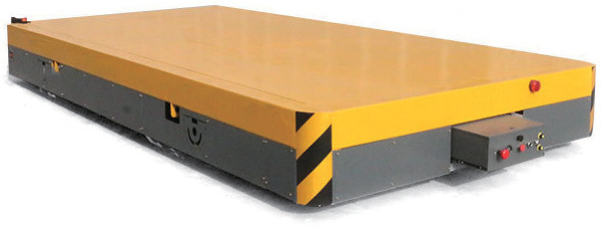
In order to verify the effectiveness of the proposed method, some experiments were organized. All experiments used the A* algorithm to plan a path. The trackless flat-handling rubber-tired vehicle shown in Figure 9 is one kind of small TRTV and is widely used in mines for handling auxiliary materials. The wheel base of this TRTV is 0.45 m, and the diameter of the four rubber wheels is 0.25 m. The length, width and height of the vehicle body are 1.20 m × 0.72 m × 0.39 m. The weight of the body is 200 kg and the theoretical load can reach 1.5 t. It can turn 360 degrees in place and climb a maximum of 20-degree slope under a light load.

The Manhattan distance shown in Equation (13) is used as the heuristic cost function in the path planning of Maps 1–6.

$$H\left(n\right)=D\times (\mathrm{abs}(n_x-goa{l}_x)+\mathrm{abs}(n_y-goa{l}_y)),$$

(13)

where $H\left(n\right)$ is the heuristic cost function. $(n_x,n_y)$ represents the coordinates of the current grid, and $(goa{l}_x,goa{l}_y)$ is the coordinates of the end point grid. D is the multiple parameter cost.

For the numerical case of Maps 7–12, the Manhattan distance is no longer the only heuristic cost, and the work done by gravity is another cost. The heuristic cost function is shown in Equation (14).

$$W\left(n\right)=\left\{\begin{array}{cc}{\displaystyle \frac{M\times g\times (G_n-G_{n-1})}{C}}\hfill & \hfill G_n>G_{n-1}\\ w\hfill & \hfill \mathrm{otherwise}\end{array}\right.,$$

(14)

where $W\left(n\right)$ is the heuristic cost function of gravity doing work. M is the weight and set in 200. g is the gravitational acceleration. $G_n$ is the height value recorded in the current grid, and $G_{n-1}$ is the height value of the previous grid. C is the normalized parameter, which is taken as 100 in this paper. w is the reward value, which is taken as $-5$ in this paper. If the height of the current grid is greater than that of the previous grid, it means that the vehicle needs to climb. At this time, the cost of gravity work of the vehicle is added to the cost of the path length. On the contrary, the vehicles are rewarded for going downhill and straight.

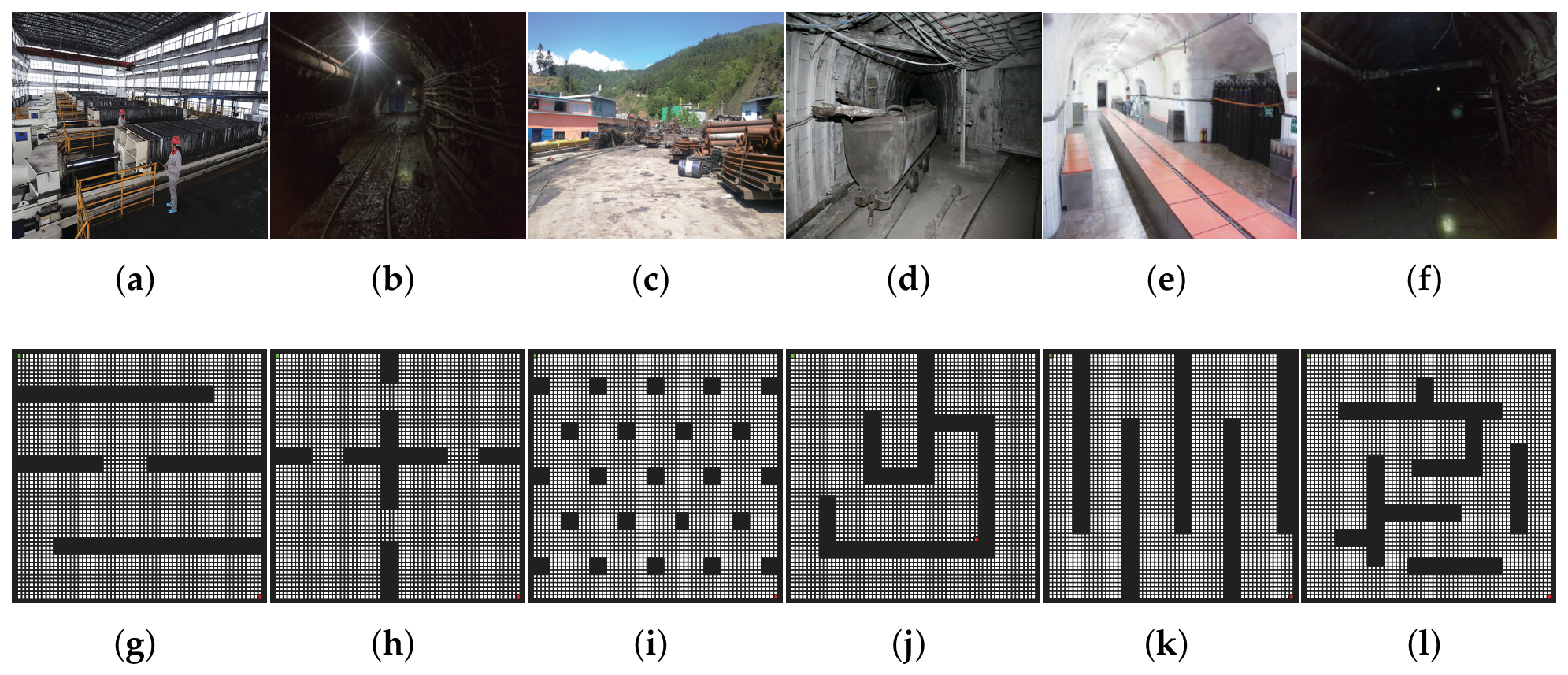
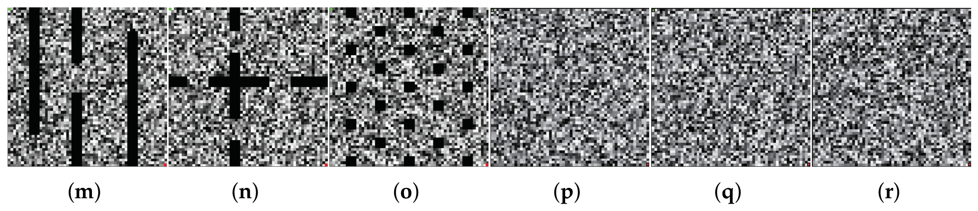
Twelve benchmark functions shown in Figure 10 with characteristics of TRTVs’ working environment are selected to test the performance of the algorithm. Figure 10a–f show the original scene of each column of the maps. Figure 10g–l are the 0–1 grid maps. The planning challenge of Map 1 in Figure 10g lies in the tortuous and constricted areas, which include small entrances and exits. Map 2 in Figure 10h can test whether the algorithm can find suitable exits and entrances in a short time. Map 3 in Figure 10i contains dense scattered obstacles, simulating bolts and anchors in the tunnel. Map 4 in Figure 10j has multiple dead-zone traps and concave spaces that are difficult to plan. Map 5 in Figure 10k shows the long and narrow tunnel that is frequently found in the working environments of TRTVs. The difficulty of Map 6 in Figure 10l is some concave spaces that are common in the underground parking yard. The others are the numerical benchmark grid maps that are divided into maps with certain obstacles and ones with irregular values, which reflect the rugged surface of the coal mine environment. In these benchmark maps, the green cell is the starting point of the vehicle, and the red cell is the end point of the task. The experimental platform and environment are shown in

Table 1. Experimental platform and environment.

Setup	Type
System	Windows 7
CPU	Intel(R) Core(TM) i5-7300HQ 2.50 GHz
RAM	8.00 GB
Software	Matlab R2014a

.

4.1. Discussion on the Performance of SIBS

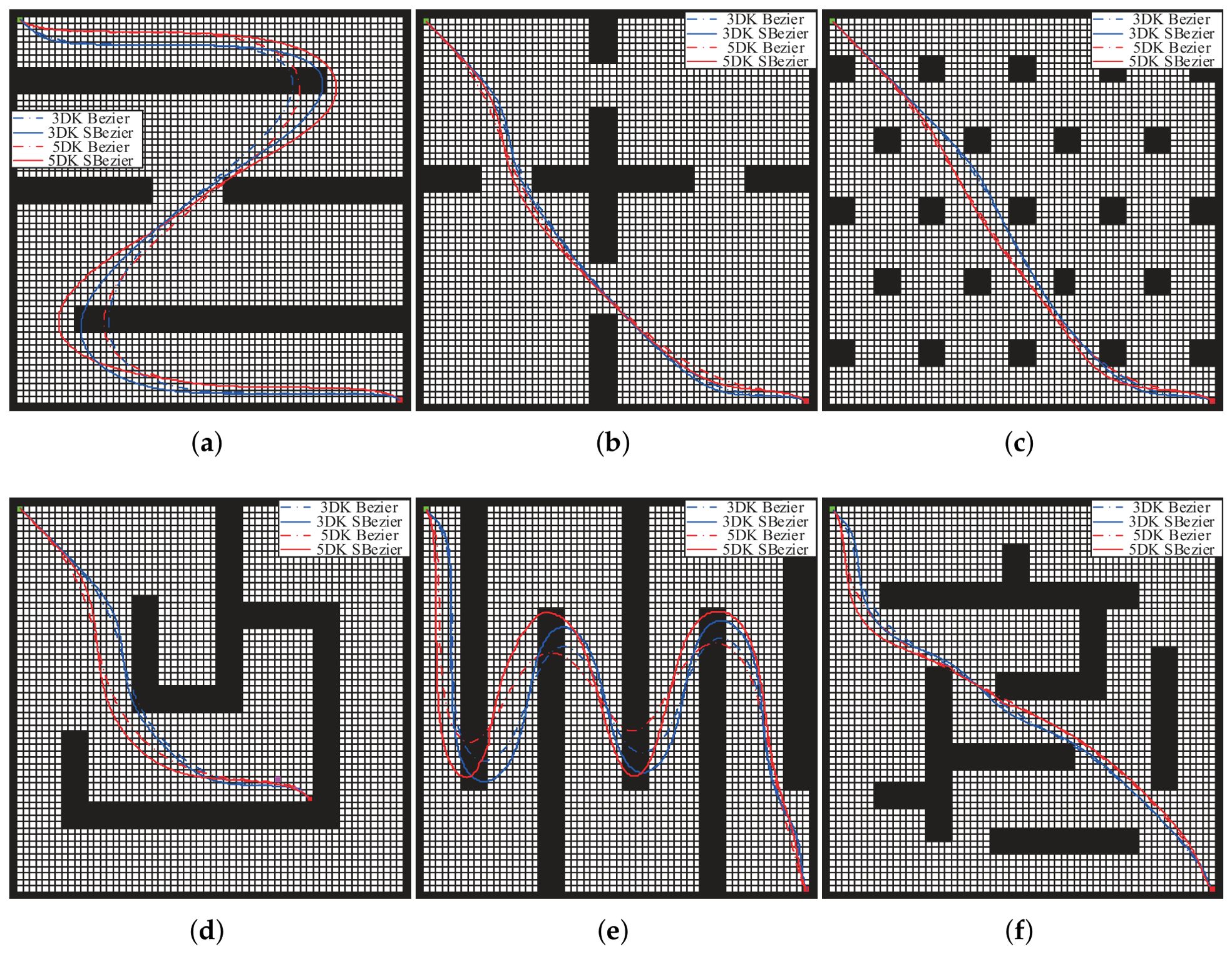
When using the shortest path as the cost function for path planning, the accessible path points planned by the algorithm are often close to the corners of obstacles resulting in frequent collisions with the smooth path. When using the proposed MDRF, this issue is further exacerbated due to fewer control points. To solve this problem, SIBS is proposed. In order to intuitively display the SIBS strategy, the comparative experiments are conducted on the six 0–1 benchmark maps. The experimental results are shown in Figure 11.

The dotted line is the result of path planning using Bezier curves, and the solid line shows the path smoothed by SIBS in Figure 11. It can be seen that the paths directly smoothed by Bezier curves have collision problems of varying degrees. However, after the SIBS is used for smoothing, the smooth path obtained has changed significantly and is collision-free in the cases except for the extremely circuitous map in Figure 11e, especially using MDRF with the 5 × 5 simplicity kernel.

4.2. Discussion on Feature Retention of Numerical Grid Map

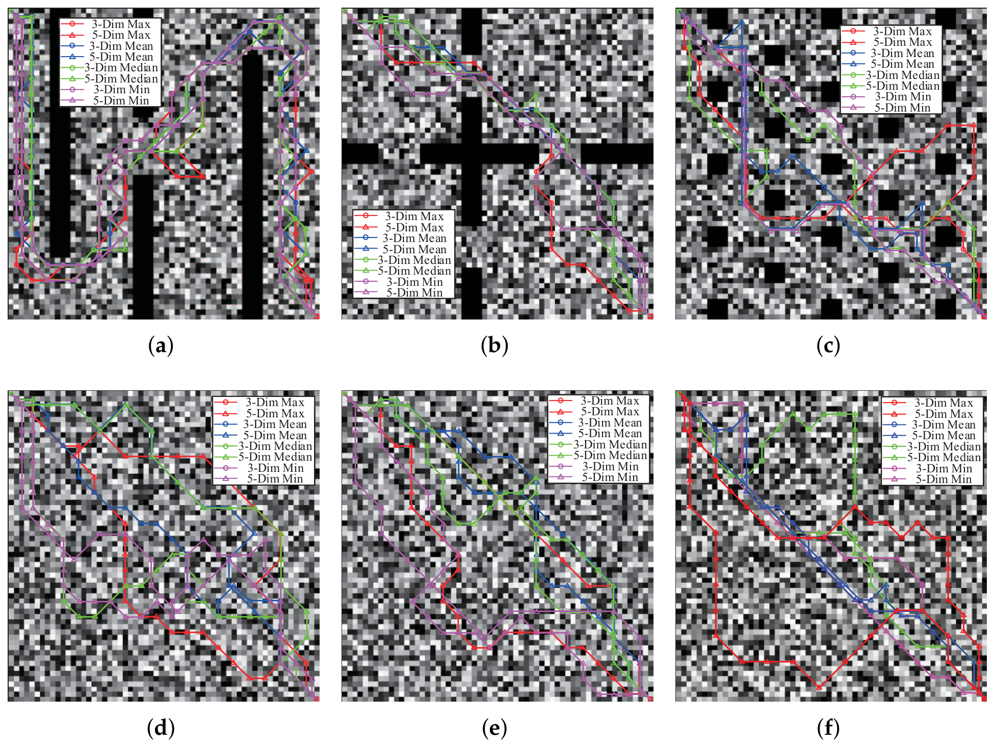
In this paper, the mean feature retention scheme in MDRF is used to reduce the dimension of the numerical grid map, but many feature retention schemes can be used in reality. In this section, the mean, the median, the maximal, and the minimal feature retention schemes are used for experiments to discuss the feasibility of different schemes. Figure 12 shows the experimental results on the six numerical grid maps, wherein the red, blue, magenta, and green smooth paths are planned on the map using MDRF with the maximal, mean, minimal, and median feature retention scheme, respectively. Two sizes of simplicity kernel are used under each scheme. It can be seen that the paths calculated with the mean value simplicity kernel have fewer twists, which means that the path length is shorter and more stable when the vehicle adopts those paths.

Table 2. Path planning cost for discussion on four feature retention schemes.

	Map 7		Map 8		Map 9		Map 10		Map 11		Map 12		Score
	$\mathit{DC}$ (m)	$\mathit{WC}$	$\mathit{DC}$ (m)	$\mathit{WC}$	$\mathit{DC}$ (m)	$\mathit{WC}$	$\mathit{DC}$ (m)	$\mathit{WC}$	$\mathit{DC}$ (m)	$\mathit{WC}$	$\mathit{DC}$ (m)	$\mathit{WC}$
3 MA	195.68	6518	104.23	4082	109.50	4137	99.98	3286	110.23	4562	110.23	4195	7
5 MA	104.23	7950	92.23	3695	143.44	4996	106.37	3978	92.23	3654	122.23	4494
3 MN	198.89	5980	98.23	3517	105.98	3545	104.23	3404	101.74	3827	102.47	3606	13
5 MN	204.65	7263	92.23	3695	122.23	4026	106.37	3017	95.15	3745	89.30	2771
3 MD	204.17	6153	102.47	3807	98.23	4186	125.74	4653	116.95	4276	124.71	4943	3
5 MD	203.44	7167	99.30	3655	122.23	3920	109.30	3575	92.23	3323	92.23	3074
3 MI	195.68	6556	96.47	3533	93.98	3629	134.23	5327	115.20	4284	86.95	2862	5
5 MI	196.37	6862	102.23	3828	108.08	3288	116.37	4326	105.15	3956	98.08	3658

shows the data results of the experiments, which can further display the effects of path planning with different feature retention schemes and simplicity kernels. Among them, MA, MN, MD, and MI represent the path planning using the maximal, mean, median, and minimal simplicity kernels, respectively. The prefixes 3 and 5 represent the 3 × 3 and 5 × 5 size of kernels. $DC$ is the path length cost and uses the meter as the unit of measure. $WC$ measures the sum of the difference between the vehicle going uphill. The size of the simplicity kernel is taken as the base for data observation, and the bold data is the best for each group of results. The “Score” is the number of wins recorded for each of the four feature retention schemes. It is obvious that the score of the mean feature retention scheme, especially the 3 × 3 mean simplicity kernels, is the highest, which is applicable to the path planning of almost every map. The maximal feature retention scheme is suitable for the numerical grid map without obstacles, and the minimal feature retention scheme is suitable for the numerical grid map with obstacles. The mean feature retention scheme is the most moderate among these four schemes. Therefore, the mean feature retention scheme is recommended and used in the final experimental comparison.

4.3. Comparative Experiments

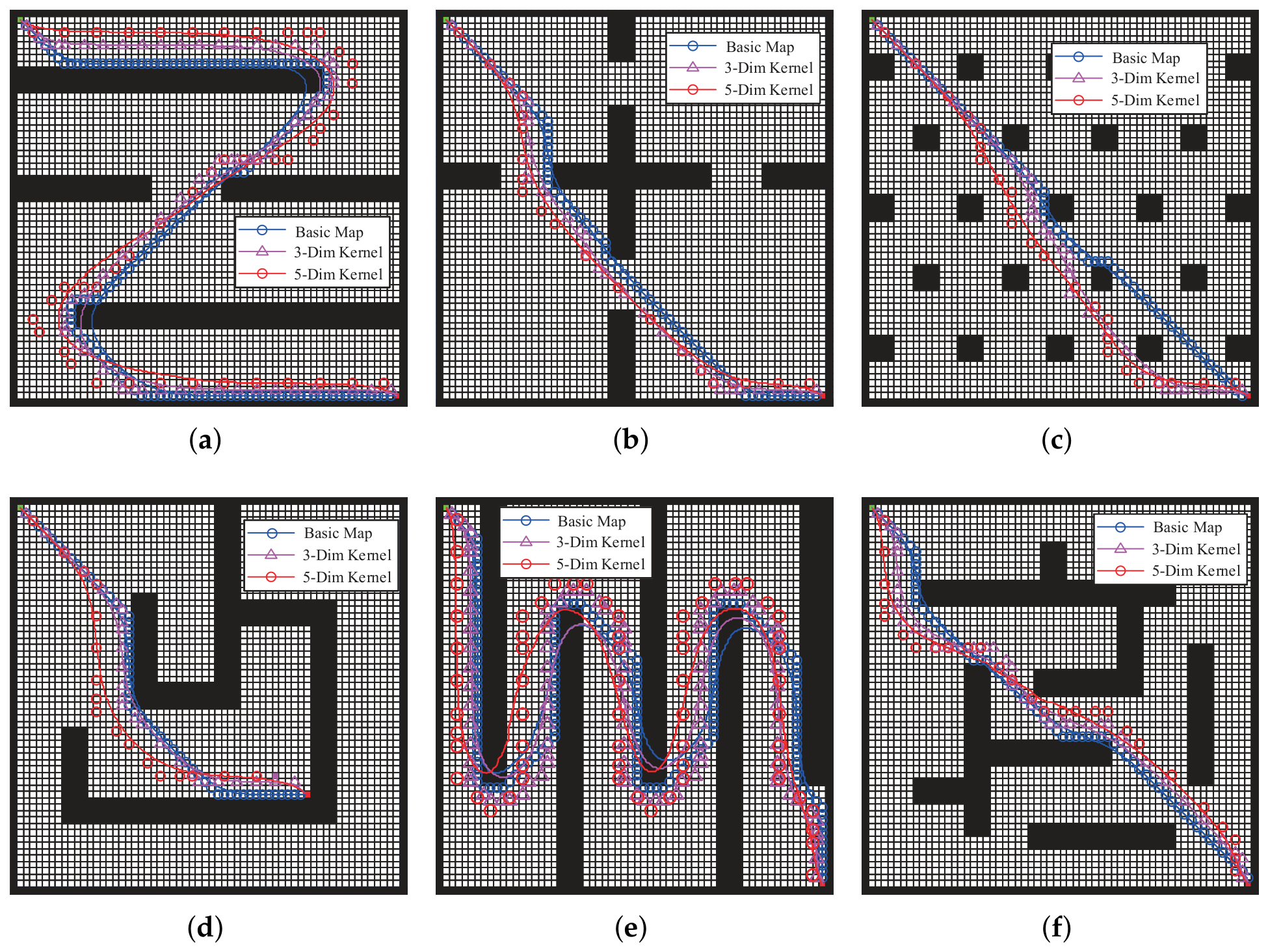
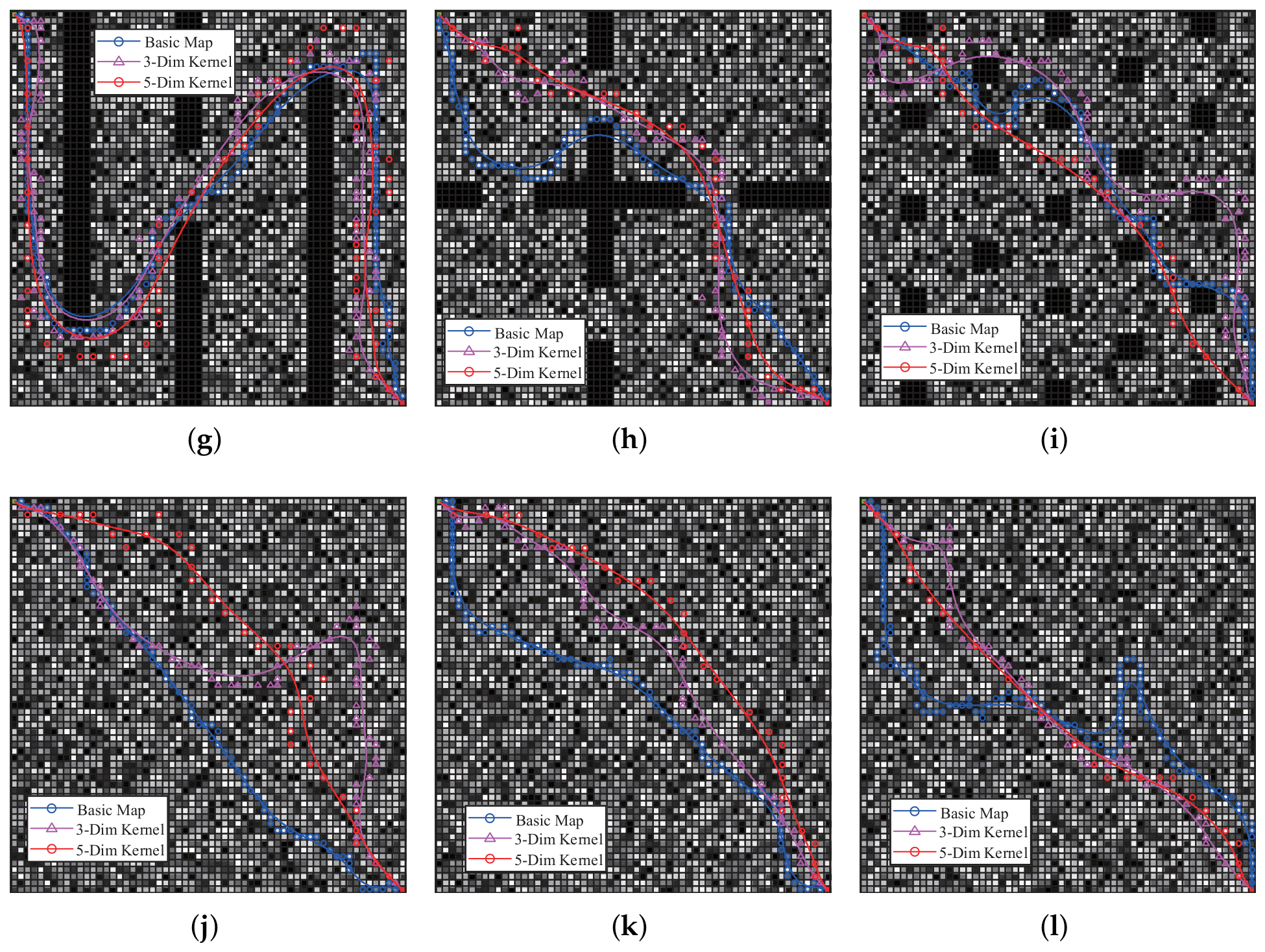
According to the above results, the basic benchmark map and the dimensionality-reduction maps are respectively used to conduct a complete experiment, and the sizes of the simplicity kernel are set as $3\times 3$ and $5\times 5$. The experimental results can be observed in Figure 13, wherein the legend, “Basic Map” denotes the planning results based on the original high-resolution map, while “3-Dim Kernel” and “5-Dim Kernel” correspond to the results of the proposed framework with 3 × 3 and 5 × 5 simplicity kernels, respectively.

In Figure 13a, the path planned on the basic map contains the largest number of control points among the three paths. Moreover, since the original path is close to obstacles, the smoothed path collides with the corners of the obstacles. On the 3 × 3 dimensionality-reduction map, the planned path possesses fewer waypoints than that on the basic map, while its smoothed path still collides with the corners of the first and last obstacles. By comparison, the path planned on the 5 × 5 dimensionality-reduction map achieves the optimal performance. Specifically, the red path has the fewest waypoints, and the corresponding smoothed path avoids all obstacle collisions. The advantages of the proposed MDRF method are also validated in the path planning results of other maps. Map 5 in Figure 13e is the most challenging one among these binary grid maps for path planning, which represents the typical winding tunnel scenarios in mine environments. The results in Figure 13e demonstrate that the path generated on the 5 × 5 dimensionality-reduction map outperforms those obtained from other maps. For the numerical grid maps with obstacles presented in Figure 13g–i, all smoothed paths planned on the dimensionality-reduction maps successfully avoid collisions with obstacle corners. Furthermore, Maps 10–12 correspond to the numerical grid maps displayed in Figure 13j–l. The paths planned on the 5 × 5 dimensionality-reduction map exhibit fewer twists and turns and better stability. In contrast, the paths generated on the basic map are extremely bumpy with numerous turns, resulting in multiple collisions on their smoothed trajectories.

The quantitative results are presented in

Table 3. Path planning cost for comparative experiments.

	Map 1		Map 2		Map 3		Map 4		Map 5		Map 6
	$\mathit{DC}$(m)	$\mathit{TC}$(s)	$\mathit{DC}$(m)	$\mathit{TC}$(s)	$\mathit{DC}$(m)	$\mathit{TC}$(s)	$\mathit{DC}$(m)	$\mathit{TC}$(s)	$\mathit{DC}$(m)	$\mathit{TC}$(s)	$\mathit{DC}$(m)	$\mathit{TC}$(s)
BM	166.95	17.36	90.47	0.75	85.78	0.41	71.84	0.41	206.47	20.59	88.71	1.19
3 DM	170.95	0.61	92.22	0.06	90.47	0.05	72.43	0.03	222.47	0.38	93.98	0.09
5 DM	186.37	0.08	92.22	0.02	92.23	0.01	73.58	0.01	229.30	0.06	95.15	0.02
	Map 7		Map 8		Map 9		Map 10		Map 11		Map 12
	$\mathit{DC}$(m)	$\mathit{TC}$(s)	$\mathit{DC}$(m)	$\mathit{TC}$(s)	$\mathit{DC}$(m)	$\mathit{TC}$(s)	$\mathit{DC}$(m)	$\mathit{TC}$(s)	$\mathit{DC}$(m)	$\mathit{TC}$(s)	$\mathit{DC}$(m)	$\mathit{TC}$(s)
BM	182.23	20.16	122.81	21.30	118.81	18.11	97.98	0.82	105.15	24.29	121.98	18.07
3 DM	198.89	0.67	98.23	0.31	105.98	0.48	104.23	0.69	101.74	0.34	102.47	0.12
5 DM	204.65	0.07	92.23	0.04	122.23	0.06	106.37	0.03	95.15	0.08	89.30	0.01

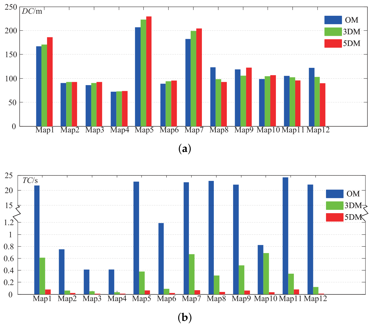
. BM denotes the results obtained from the basic map, while 3DM and 5DM correspond to the results on the 3 × 3 and 5 × 5 dimensionality-reduction maps, respectively. $DC$ represents the path length cost in meters, and $TC$ denotes the computational runtime cost in seconds. The results indicate that the basic map yields the shortest planned path length, whereas the 5 × 5 dimensionality-reduction map achieves the minimum planning runtime, with a runtime reduction of approximately $90\%$ across all 0–1 grid maps. Accordingly, the experimental results on 0–1 grid maps demonstrate that as the dimension of the simplification kernel increases, the path length cost increases slightly, while the planning time cost decreases significantly. For numerical grid map experiments, the 5 × 5 simplification kernel applied to basic maps achieves the optimal comprehensive path planning performance in terms of both path length and computational efficiency. The effectiveness and superiority of the proposed MDRF method can be further intuitively verified from the results in Figure 14.

4.4. Discussion on the Safety of the Path

Safety is necessary for the vehicle path planning in coal mines according to the relevant ongoing national standards [41], industrial standards [42,43] and local standards [44,45] of coal mine transportation and intelligent coal mine auxiliary transportation equipment management. There are obvious differences between the coal mine environment and the ground. The underground environment is of high gas concentration, limited space, easy collision, and low illumination, which makes the safety and lightweight requirements for TRTVs very high. Moreover, the occurrence of safety accidents makes it easy to cause large-scale chain disasters, so the optimal path length can only be used as one of the reference standards, and the safety of the planned path also needs to be evaluated.

From the above experiments’ results, it can be observed that the proposed method in this paper sacrifices the optimality of the path length in exchange for lightweight and planning time. The experiments in this section will discuss the safety of the planned path on the map after dimensional reduction using the proposed method.

From Figure 13a–f of the comparative experiments in Section 4.3, it is observed that the path planned on the basic maps is close to the obstacles, while the ones planned on the map using the method in this paper mostly obtain path points with a certain distance from obstacles. In the confined space of a deep well, multiple small and risky obstacles are not easy to detect around the conspicuous obstacles, e.g., puddles, anchor rod after a shadow, etc. Therefore, we hope that the path of the TRTVs can keep away from obstacles as far as possible while keeping the short length. The path planning on the map using the modification method just meets the requirements of mining vehicles, and the path length cost is slightly increased to less than $1\%$ as shown in Table 3.

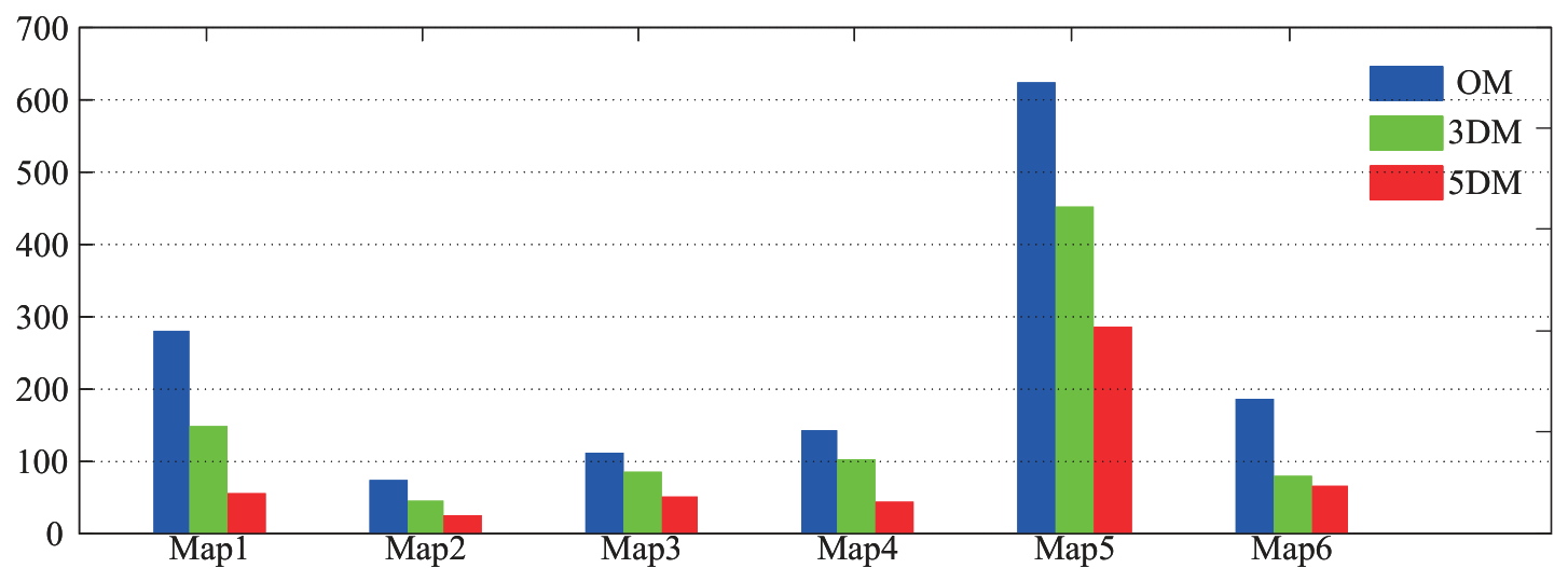
To scientifically determine whether the path is safe, the risk map evaluation method that we proposed in 2023 [2] is used to visually assess the safety of the path, and the risk value of each path is counted. The results are shown in

Table 4. The risk value of the path.

	M1	M2	M3	M4	M5	M6
BM	280	70	109	142	628	181
3 DM	146	46	94	101	449	91
5 DM	71	31	52	42	294	80

and Figure 15, wherein M1–M6 represent Maps 1–6 respectively. It is clear that the path planned on the map using 5 × 5 MDRF has minimal risk value.

4.5. Downhole Map Experiment

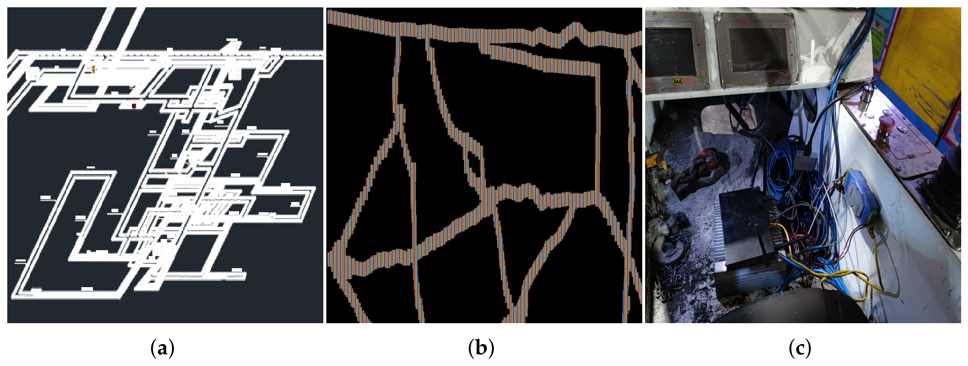
To further verify the feasibility of the proposed method, a downhole map obtained from the partial tunnel network of a mine in southwestern China was used as shown in Figure 16. The downhole tunnel network is often complex, generally consisting of a main transportation tunnel and multiple tunnels leading to the mining face. Temporary tunnels reaching the mining face frequently change with the progress of mining, so compared to ground roads, there is no regular pattern. The underground tunnel network usually includes multiple downhole parking lots. The map used this time includes the main transportation tunnel and some temporary tunnels. The hardware, computing units and industrial control computers were the ones used in our previous downhole experiments [5], as shown in Figure 16c. A customized industrial computer, model Tardetech TD-WUFO-8100G, was used. The CPU was Core i7-9700 with two 32 GB industrial RAM, one 512 GB industrial SSD, 24 G RTX-3090 GPU, etc., which are equipped with and packaged in an explosion-proof shell. CAN and high-speed Ethernet are used to achieve data and signal communication. The Ubuntu 20.04 operating system is used.

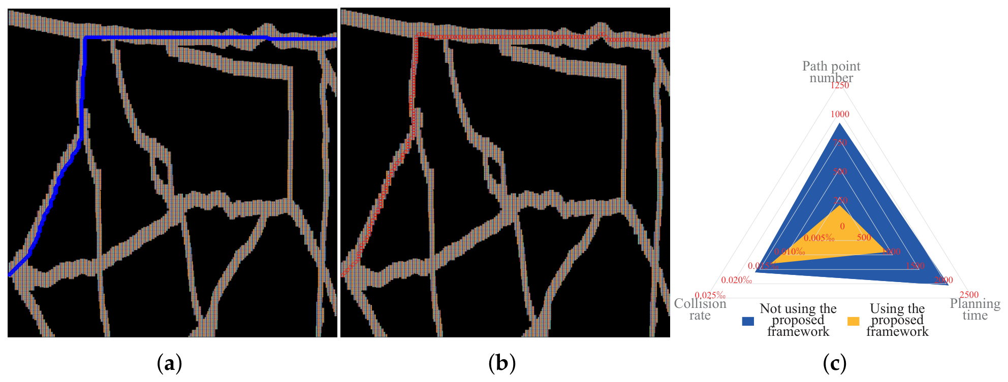
As shown in Figure 17, path planning based on the original map requires a planning time of 2058.4 s and generates more than 894 path points with obvious redundancy. In comparison, the planning method adopting the 5 × 5 simplification kernel only produces 180 path points within 4.7 s. Compared with the original map-based planning strategy, the proposed method reduces the planning time by 99.8% and cuts down redundant path points by 79.6%, which demonstrates a significant improvement in planning efficiency. Furthermore, two groups of path points are smoothed separately using the original Bezier algorithm and the improved smoothing method proposed in this framework. The total number of smoothing points is set to 10,000. The collision rate of the smoothed path is calculated by dividing the number of smoothing points located in obstacle grids by the total number of smoothing points. As illustrated in Figure 17c, the collision rate of the smoothed path points optimized by our proposed method is 0.13‰, while that obtained without the dimensionality-reduction framework is 0.16‰. This indicates that the proposed framework effectively eliminates potential collision risks by optimizing the number of smoothing reference points.

5. Conclusions

This work targets the efficiency and safety improvement of intelligent coal mine TRTVs by optimizing grid map representations, and proposes a multi-scale dimensionality-reduction framework to eliminate redundant map information and accelerate path planning. Designed for the limited onboard computing resources of underground vehicles, MDRF adaptively downsamples high-resolution maps to support reliable TRTV navigation. Evaluations on twelve benchmark maps confirm that MDRF reduces planning time by more than 90% while ensuring safe and smooth paths. Among four designed feature retention schemes for the simplification kernel, the mean-value scheme achieves the most balanced performance. Practical tests on real downhole mine maps further demonstrate that the proposed method reduces planning time by 99.8% and redundant path points by 79.6%. Equipped with an improved smoothing strategy, the framework effectively avoids collision risks caused by insufficient path reference points. Owing to its adaptability to environments with limited sensor precision, power supply, and computing resources, MDRF serves as a universal preprocessing module that can be seamlessly combined with mainstream planners such as A* and RRT. Future work will explore advanced feature retention strategies to boost dimensionality-reduction accuracy and extend the current framework to 3D mine maps for wider engineering applicability.