Research on a Dynamic Prediction Method for Rainstorm Disaster Chains Based on LLM-Optimized Sliding Window and Dynamic Bayesian Network

Abstract

Rainstorm-induced disaster chains are characterized by high suddenness, immense destructive power, and complex chain propagation mechanisms. Traditional static assessment methods rely on fixed parameters and struggle to depict the dynamic evolution of such disasters. Existing dynamic models are mostly based on predefined structures and lack the capability to integrate multi-source data and quantify uncertainty, thereby constraining the accurate prediction of rainstorm disaster chains. To address these issues, this study proposes a rainstorm disaster chain prediction model (SW-DBN) that integrates a large language model (LLM)-optimized sliding window mechanism with a dynamic Bayesian network (DBN). The model first performs dynamic segmentation and feature extraction on multi-source time-series data through the sliding window mechanism and constructs an LLM-driven module for semantic understanding of multi-source information and latent parameter mining. By leveraging the LLM’s in-depth analysis of data pattern variations within the window, the model excavates latent parameters, adaptively adjusts the DBN network topology, and feeds back to optimize the window width and sliding step, thereby maintaining adaptive alignment between the sliding window’s feature extraction and the dynamic evolution of the disaster chain. Ultimately, the cascade propagation process of the rainstorm disaster chain is modeled, reasoned, and validated through the DBN, forming an integrated prediction framework of “perception–reasoning, dynamic regulation, and cascade verification.” A case study in the Xi’an area demonstrates that the proposed model can effectively simulate the temporal evolution of rainstorm disaster chains. The average prediction accuracy for four key types of disaster nodes reaches 84.8%, representing an improvement of 7.5 percentage points over the standard DBN model, with clear advantages in early warning timeliness for critical nodes. The proposed model provides technical support for the probabilistic prediction of rainstorm disaster chains and disaster prevention decision-making, featuring both dynamic adaptability and interpretability.

1. Introduction

Against the backdrop of global climate change, the frequency and intensity of extreme rainfall events have been continuously increasing [1], inducing secondary disasters such as landslides, debris flows, flash floods, and waterlogging with growing frequency, and these disasters exhibit pronounced compounding and chain evolution characteristics [2,3,4,5]. Rainstorm disaster chains are highly sudden and destructive, with cascade propagation processes characterized by strong temporal coupling and high state uncertainty [5,6].

Regarding the prediction of rainstorm disaster chains, existing studies have explored approaches such as multi-hazard coupling analysis and dynamic probabilistic graphical modeling [7,8,9]. In disaster chain modeling, Bayesian Networks (BNs), owing to their ability to structurally express multi-factor dependencies, have been used for constructing static disaster chain structures and identifying key factors [8,10,11]. To further characterize the temporal evolution of disasters, dynamic Bayesian networks (DBNs) extend static structures into a dynamic reasoning framework by introducing time slices and state transition mechanisms [12,13,14]. However, traditional static risk assessment methods, which rely on fixed parameters and structures, find it difficult to capture the continuous propagation of disasters over time. Although existing dynamic models enhance temporal modeling capability by incorporating time slices, most define state transition relationships based on predefined structures or expert experience, lacking the ability to deeply analyze and adaptively integrate implicit evolution patterns from real-time rainfall variations and multi-source heterogeneous monitoring data. This results in limited prediction accuracy and update efficiency in complex dynamic scenarios [14,15,16].

Large language models (LLMs) possess powerful semantic parsing and data mining capabilities, enabling them to extract latent parameters from multi-source time-series data. They have already shown potential in disaster chain relationship identification and rapid disaster assessment [17,18,19,20]. For example, Zhou et al. [19] used LLMs to extract multi-hazard events related to tropical cyclones from official disaster records, successfully identifying chain relationships such as precipitation–flood–storm surge. Wang et al. [20] combined LLMs with crowdsourced data to achieve rapid estimation of earthquake-induced casualties, verifying the feasibility of LLMs in disaster probabilistic reasoning. In the broader context of temporal prediction, recent studies have demonstrated that fusing temporal and contextual features from heterogeneous urban datasets can substantially improve prediction accuracy. For example, Balderas-Díaz et al. [21] proposed a context-aware framework that integrates temporal and contextual features for traffic volume prediction, achieving competitive performance through direct feature fusion. The proposed SW-DBN model focuses on rainstorm disaster chain prediction, where explicitly capturing causal relationships among cascading events is essential. To address this, the model introduces LLM-driven causal structure mining, which extracts latent parameters from multi-source time-series data and dynamically updates the DBN topology and conditional probability tables. However, how to organically integrate the data mining strengths of LLMs with the temporal probabilistic reasoning capability of DBNs, overcome the limitations of static assessment and dynamic models with predefined structures, and construct a rainstorm disaster chain prediction method that can integrate multi-source information and possesses dynamic adaptive ability remains an urgent problem in the field of disaster prevention and mitigation.

To address this, the paper proposes a rainstorm disaster chain prediction model (SW-DBN) that integrates an LLM-optimized sliding window mechanism with a DBN. The model segments multi-source time-series data through the sliding window, employs the LLM to mine latent parameters for adaptively adjusting the DBN network topology and feeding back to optimize window parameters, and then conducts reasoning and validation of the cascade propagation process through the DBN, forming an integrated framework of “perception–reasoning, dynamic regulation, and cascade verification.” This model provides methodological support that combines dynamic adaptability and interpretability for the dynamic prediction of rainstorm disaster chains.

2. Materials and Methods

2.1. Study Area and Data

2.1.1. Study Area

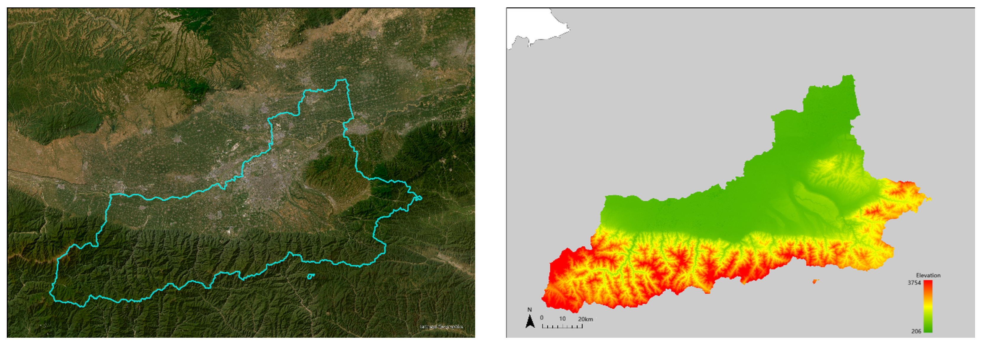
Xi’an is located at the northern foot of the Qinling Mountains, with a distinctive geomorphological pattern characterized by “steep terrain in the south and flat terrain in the north.” The southern mountainous area is dominated by loess hills, valley terraces, and mountains [22], where intense rainfall can easily trigger geological disasters such as flash floods, landslides, and debris flows. The northern urban area sits on a plain basement but is influenced by micro-undulating terrain formed by multiple east–west trending slopes, leading to concentrated water accumulation in low-lying areas and a prominent risk of waterlogging [23,24]. The region has a warm temperate semi-humid continental monsoon climate with uneven spatiotemporal distribution of precipitation. Summer rainstorms are frequent and intense, with highly concentrated short-duration heavy rainfall events. This geographic pattern causes geological disasters in mountainous areas and urban waterlogging to often occur simultaneously or in chains, forming compound disaster chains that significantly amplify disaster impacts. The Xi’an area is shown in Figure 1.

Driven by intense rainfall, the Xi’an area predominantly develops typical compound disaster chains such as “rainstorm–landslide–debris flow,” “rainstorm–flash flood–waterlogging,” and “rainstorm–waterlogging–infrastructure damage.” Among these, the loess landslide–debris flow disaster chain and the flash flood–waterlogging chain are particularly prominent, making the region a representative case for studying rainstorm disaster chains.

2.1.2. Data

To support the LLM in semantic parsing of rainstorm disaster chain evolution patterns and latent parameter mining, this study, drawing on the analysis of 85 typical disaster events from 2016 to 2023 by Zhao et al. [9] and considering the regional characteristics of rainstorm disaster chains in Northwest China, collected multi-source spatiotemporal data. In accordance with the input requirements of the LLM and the principle of data synergy and fusion, the data are categorized into three types: meteorological time-series data, spatial background data, and disaster semantic data.

The meteorological time-series data consist of two tiers: (1) approximately 1.35 million hourly monitoring records from 188 high-density rainfall stations in the Xi’an area since July 2025, providing fine-grained spatial coverage for the most recent period; and (2) historical daily and hourly rainfall records at the district/county level from 2007 to June 2025, obtained from the China Meteorological Administration through online data services, which provide coarser but sufficient temporal context for long-term disaster chain pattern mining, covering key indicators such as hourly rainfall and cumulative rainfall, thereby providing high-temporal resolution input for dynamic parsing through the sliding window. The spatial background data include derived attributes such as slope and aspect generated from a 30 m resolution DEM of the Xi’an area, combined with information on 4190 river segments, water supply networks, municipal roads, bridges, drainage outlets, reservoirs, and other infrastructure, along with prior information on 569 disaster risk points and 632 geological hazard potential points. Together, these characterize the regional hazard-prone environment and the spatial pathways of disaster chain propagation. The semantic disaster data include 896 structured disaster event records and 123 unstructured text disaster reports spanning nearly two decades, providing a knowledge reference for semantic understanding and latent parameter mining within the LLM’s sliding window. After uniform spatial registration, the above data were used to construct continuous multivariate time series at an hourly scale, with missing values and outliers handled by linear interpolation and Kriging interpolation, respectively.

2.2. Methods

2.2.1. Overall Framework of the SW-DBN Model

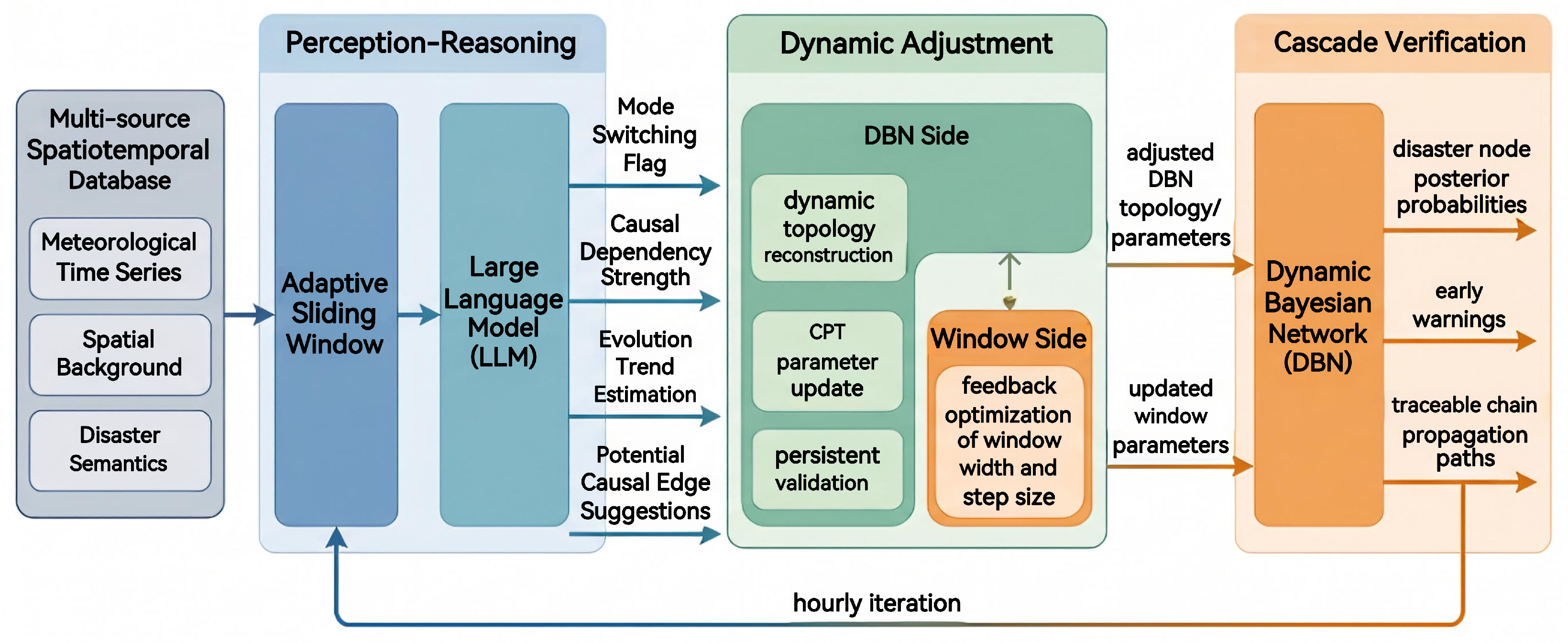
To address the challenges of strong multi-source information heterogeneity, distinct temporal phasing, and complex cascade propagation mechanisms during the evolution of rainstorm disaster chains, this paper proposes a dynamic prediction model for rainstorm disaster chains that integrates an LLM-optimized sliding window mechanism with a dynamic Bayesian network (SW-DBN). The model operates along a three-stage pathway of “perception–reasoning, dynamic regulation, and cascade verification.” In the perception–reasoning stage, the model takes a multi-source database as input, dynamically segments meteorological time-series, spatial background, and disaster semantic data through an adaptive sliding window, and invokes the LLM to deeply parse data pattern variations within the window, thereby mining four types of latent parameters: pattern switching indicators, causal dependency strengths, evolution trend estimates, and potential causal edge suggestions. In the dynamic regulation stage, these latent parameters are received, and bidirectional adaptive adjustment is performed. On the DBN side, pattern switching indicators and causal dependency strengths are used to dynamically reconstruct the network topology, update conditional probability table parameters, and screen potential causal edges through persistence validation; on the window side, the window width and sliding step are feedback-optimized based on evolution trend estimates. In the cascade verification stage, based on the adjusted DBN topology and parameters, a dynamic Bayesian network incorporating state nodes such as landslide, debris flow, flash flood, and waterlogging, along with evidence nodes such as temporal drivers and spatial background, is constructed to output posterior probabilities for each disaster node, early warning signals, and traceable chain propagation paths. These three stages iterate cyclically on an hourly basis, with the data flow and functional coupling among modules illustrated in Figure 2.

2.2.2. Data Processing and Database Construction

The multi-source data collected in this study, encompassing meteorological time-series, spatial background, and disaster semantic data, provide the foundation for constructing the SW-DBN model. However, the raw data suffer from issues such as multi-source heterogeneity, spatiotemporal inconsistency, missing values, anomalies, and semantic unstructuredness. Specifically, data formats including hourly rainfall records from meteorological stations, river network vectors, DEM rasters, disaster point coordinates, and unstructured text vary considerably, making direct integration difficult. Spatiotemporal resolutions from different sources are mismatched: rainfall data are point-based hourly records, whereas geological hazard potential points are static coordinates, and disaster event texts lack precise timestamps. Some rainfall stations experienced data loss due to communication disruptions during extreme rainfall, and individual monitoring records exhibit abrupt jumps caused by sensor malfunctions. Moreover, chain propagation descriptions in news reports and disaster investigation reports are difficult to directly use for probabilistic modeling and must be converted into structured information.

To address these issues, this study systematically preprocessed the raw data. In the spatial dimension, vector and raster data such as DEM, rivers, and infrastructure were uniformly projected to the WGS84 coordinate system and resampled to a 30 m × 30 m grid. Meteorological station data were interpolated using inverse distance weighting to generate grid-aligned areal data, and the coordinates of disaster risk points and potential hazard points were spatially joined and assigned to the nearest grid cells. In the temporal dimension, a continuous time series was constructed with an hour as the basic time step. Single-point missing intervals of less than three consecutive hours were filled using linear interpolation, while missing segments exceeding three hours were backfilled using Kriging interpolation with data from neighboring stations after spatial estimation. Outlier detection employed $3\sigma$ principle: values exceeding the historical mean for the same period by ±3 standard deviations were flagged as outliers and treated as missing values. In the semantic dimension, for the 896 structured historical disaster records, fields such as disaster type, occurrence time, triggering conditions, and chain propagation paths were directly extracted to construct a disaster event relationship table. For the 123 unstructured texts, a hybrid NER-RE pipeline was employed. Named Entity Recognition was performed using a BERT-BiLSTM-CRF architecture fine-tuned on a disaster-domain annotated corpus, extracting four entity types: disaster type (e.g., landslide, debris flow, flash flood, waterlogging), location (administrative district, geographic feature), time expression, and triggering condition (e.g., heavy rainfall, soil saturation). The fine-tuned model achieved an entity-level F1 score of 0.91 on a held-out test set of 30 manually annotated reports. For Relation Extraction, a two-stage approach was adopted: first, rule-based pattern matching with 12 hand-crafted dependency templates (e.g., “X triggered Y,” “X transformed into Y,” “due to X, Y occurred”) was applied to extract high-confidence causal pairs; second, a BERT-based sentence-pair classifier was used to verify candidate relations from reports where rule-based extraction produced incomplete results, with only relations scoring above a confidence threshold of 0.8 being retained. All extracted triples were manually reviewed by two annotators (inter-annotator agreement: Cohen’s $\kappa =0.87$), and disagreements were adjudicated by a third senior expert. The final knowledge graph contains 423 verified causal triples. The extracted causal pairs were formed into standardized chain descriptions such as “rainstorm → landslide” and “landslide → debris flow,” which were stored in a disaster knowledge graph.

After preprocessing, a dedicated multi-source spatiotemporal database for the SW-DBN model was constructed. This database comprises three sub-databases: the meteorological time-series sub-database stores hourly rainfall, cumulative rainfall from 188 stations, and the interpolated grid sequences; the spatial background sub-database stores static and quasi-static layers such as 30 m resolution DEM, slope, aspect, river buffer zones, drainage outlet density, road networks, risk points, and potential hazard points; and the disaster semantic sub-database stores the structured disaster event table and the disaster chain knowledge graph, supporting LLM prompt-based retrieval. The three sub-databases are linked through unified grid codes and time indices to enable associative queries, providing data input for the adaptive sliding window in the perception–reasoning stage.

In addition to the data stored in the database, a candidate causal edge set ${\mathcal{E}}_{candidate}$ was also constructed to constrain the initial search space of DBN structure learning, thereby avoiding spurious connections with inverted causality such as “waterlogging → rainfall.” In its initial state, it includes four basic types of causal relationships: rainfall triggering (e.g., “rainfall → landslide,” “rainfall → waterlogging”), disaster type transformation (e.g., “landslide → debris flow”), hydrological conveyance (e.g., “flash flood → waterlogging”), and disaster amplification (e.g., “waterlogging → infrastructure failure”).

2.2.3. Perception–Reasoning: Adaptive Sliding Window and LLM Latent Parameter Mining

The perception–reasoning stage is built upon the multi-source spatiotemporal database and consists of the collaborative operation of an adaptive sliding window and LLM-based latent parameter mining. In this stage, an adaptive sliding window is constructed with the current moment as the reference point. Hourly rainfall and cumulative rainfall are extracted from the meteorological time-series sub-database; static attributes such as slope, aspect, distance to rivers, and drainage outlet density are extracted from the spatial background sub-database; and historical disaster event chain records and the knowledge graph are extracted from the disaster semantic sub-database. The multi-source information within the window is encapsulated into structured text blocks and, together with disaster knowledge data, organized into a prompt template, which is then input into the DeepSeek-R1-14B model to mine four types of latent parameters: pattern switching indicators, causal dependency strengths, evolution trend estimates, and potential causal edge suggestions. The initial window length and step size are set based on the temporal statistical characteristics of rainstorm events within the study period and are subsequently optimized through feedback from the dynamic regulation stage.

During the sustained rainfall phase of a rainstorm disaster chain, monitoring indicators change gently, whereas abrupt shifts occur at the disaster triggering stage. A fixed time window struggles to accommodate both types of characteristics: an overly wide window smooths out abrupt change signals, causing prediction delays, while an excessively narrow window amplifies noise, triggering false alarms. Taking a typical rainstorm disaster chain in Xi’an on 16 September 2025 (hereinafter referred to as the “Xi’an 9.16 Rainstorm Disaster Chain”) as an example: when a fixed 6 h window was used, the first three hours of the window prior to sustained rainfall contained a large amount of steady data, which overwhelmed the information of the subsequent sharp increase in rainfall intensity, causing the model’s predicted peak of landslide occurrence probability to be delayed by approximately two hours relative to the actual occurrence time. In contrast, when a fixed 2 h window was used, random fluctuations during the steady phase frequently triggered pattern switching, leading to repeated reconstruction of the DBN topology, wasted computational resources, and reduced prediction stability. Therefore, there is a need for an approach that can adaptively adjust the window length according to the intensity of data changes and employ the LLM to mine latent parameters from the multi-source data within the window that are difficult to extract using conventional statistical methods. Hence, the evolution process of a rainstorm disaster chain is represented as a multi-source observation time series:

$$\mathcal{X}=\left\{x_1,x_2,\dots ,x_T\right\}$$

(1)

Here, $x_t$ denotes the multi-source observation information set at time t, specifically including the hourly rainfall $R_t$ and cumulative rainfall $C_t$ from the meteorological time-series sub-database, static attributes from the spatial background sub-database (such as slope G, distance to river $D_{river}$, drainage outlet density $D_{drain}$, etc.), and the disaster state records from the previous time step (binary states of landslide, debris flow, flash flood, and waterlogging). To enable adaptive window adjustment and subsequent LLM parsing, the multi-source heterogeneous observations $x_t$ are uniformly represented as a vector, where numerical monitoring data are normalized as $v_t^{num}$, disaster state records are represented as a binary vector $v_t^{state}$, and static spatial attributes as $v^{spatial}$. Thus, the structured representation at time t can be written as $x_t=[v_t^{num};v_t^{state};v^{spatial}]$. The change intensity indicator between adjacent moments is defined as

$$S_t=1-sim(x_t,x_{t-1})$$

(2)

Here, $sim(·)$ denotes the cosine similarity. A large $S_t$ indicates significant differences between adjacent moments, suggesting that the system may be in a disaster triggering or rapid evolution phase; a small $S_t$ indicates relatively stable system changes.

The window length is dynamically adjusted using an exponential decay strategy based on the change intensity:

$$L_t=\mathrm{round}\left(L_{min}+(L_{max}-L_{min})·e^{-\lambda S_t}\right)$$

(3)

Here, $\lambda >0$ is the decay coefficient that controls the sensitivity of the window length to the change intensity. $L_{min}$ and $L_{max}$ denote the minimum and maximum window lengths, respectively. The initial values of $L_{min}$, $L_{max}$, and $\lambda$ are set based on the temporal statistical characteristics of rainstorm events within the study period: $L_{min}$ references the typical duration of a single short-duration heavy rainfall event, $L_{max}$ references the average impact duration of a complete rainstorm process, and $\lambda$ is calibrated using the change intensity distribution of historical events such that when $S_t$ takes the historical mean, the window length output by Formula (3) approximates ${\displaystyle \frac{L_{min}+L_{max}}{2}}$. Accordingly, the context at time t can be expressed as

$$W_t=\{x_{max(1,t-L_t+1)},x_{max(1,t-L_t+2)},\dots ,x_t\}$$

(4)

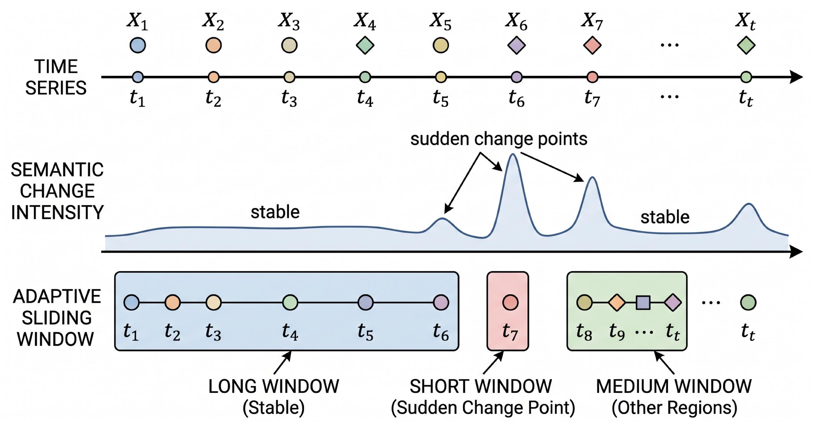
As shown in Figure 3, each window $W_t$ constitutes a context unit with semantic integrity.

Corresponding to the window length, the sliding step $H_t$ determines the interval between the start times of two adjacent windows. An excessively large step may cause information jumps between windows, potentially missing critical evolution stages, whereas an excessively small step increases computational redundancy. This study sets the initial step $H_0=3$ h, which is subsequently feedback-optimized by the dynamic regulation stage based on the evolution trend. After the inference of the current window is completed, the start time advances by the step size to $t+H_t$, entering the next round of perception–reasoning, thereby forming continuous temporal coverage.

After the window is constructed, the time-series numerical records, disaster state sequences, and spatial attributes for the corresponding period within it are uniformly encapsulated into a structured text block $T_t$. $T_t$ is then organized together with historical disaster records and news report texts from the disaster knowledge data into a prompt template, which is input into DeepSeek-R1-14B for in-depth parsing [25]. Upon receiving the prompt, the model first identifies the phasing of the rainfall process within the window, then compares the current multivariate evolution trajectory with typical chain triggering patterns by referencing the historical disaster chain case database and finally generates four types of latent parameters according to a predefined output format. Through this parsing, the LLM obtains the following latent parameters from the window data that are difficult to directly acquire using conventional methods:

(1)

Pattern switching indicator ${\delta }_t\in 0,1$: indicates whether the system has entered a new evolution phase.

(2)

Causal dependency strength ${\rho }_{ij}^{\left(t\right)}\in [0,1]$: infers the closeness of causal associations between disaster nodes under the current window context.

(3)

Evolution trend estimate ${\tau }_k^{\left(t\right)}\in \mathrm{rising},\mathrm{stable},\mathrm{declining}$: provides the future tendency of disaster state nodes, used for feedback optimization of window parameters in the dynamic regulation stage.

(4)

Potential causal edge suggestions ${\mathcal{E}}_t^{new}$: identifies potential causal relationships not yet included in the candidate structure set ${\mathcal{E}}_{candidate}$ but supported by the window data patterns.

To ensure the LLM-derived latent parameters are formally grounded and numerically compatible with DBN computation, each parameter type undergoes a constrained derivation pipeline. For the pattern switching indicator ${\delta }_t$, the LLM compares the current window’s rainfall intensity trend and disaster state vector against a predefined set of phase-transition templates extracted from historical disaster events, outputting a binary decision with a confidence score; ${\delta }_t$ is set to 1 only when the confidence exceeds 0.8, otherwise it defaults to 0. The causal dependency strength ${\rho }_{ij}^{\left(t\right)}$ is obtained through a semantic-to-numerical mapping: the LLM first evaluates the co-occurrence frequency, temporal precedence, and physical mechanism plausibility of each candidate edge within the window context, then projects the qualitative assessment onto a $[0,1]$ scale via a structured scoring rubric with five ordinal levels (very weak = 0.1, weak = 0.3, moderate = 0.5, strong = 0.7, very strong = 0.9), with intermediate values produced by linear interpolation. Evolution trend estimates ${\tau }_k^{\left(t\right)}$ are derived from the slope direction and magnitude of the disaster node’s posterior probability trajectory within the window, discretized into three categories based on a minimum slope threshold ${\theta }_{slope}$. Potential causal edge suggestions ${\mathcal{E}}_t^{new}$ are generated only when the LLM identifies a statistically anomalous co-variation pattern between two nodes that cannot be explained by existing edges, and the suggestion is required to cite specific data evidence (e.g., rainfall runoff anomalies, sensor readings) from the window in its reasoning trace. All outputs are validated against a JSON schema before acceptance; any parameter violating type, range, or format constraints is rejected and re-queried. This formalized pipeline ensures that LLM outputs are not free-text opinions but constrained, verifiable numerical parameters suitable for DBN integration.

The above four types of latent parameters, after formalized encoding, are simultaneously passed to the dynamic regulation stage: ${\delta }_t$, ${\rho }_{ij}^{\left(t\right)}$, and ${\mathcal{E}}_t^{new}$ are used for adaptive adjustment of the DBN topology and parameters, while ${\delta }_t$ and ${\tau }_k^{\left(t\right)}$ are used for feedback optimization of the window width and sliding step. Through the LLM’s in-depth parsing of window data patterns, latent evolution features that are difficult to explicitly model using traditional statistical methods can be extracted, thereby significantly improving the model’s depiction accuracy and prediction precision for the evolution process of rainstorm disaster chains.

2.2.4. Dynamic Regulation: Latent Parameter-Driven Bidirectional Adaptive Adjustment

The dynamic regulation stage receives the four types of latent parameters output by the LLM in the perception–reasoning stage and performs adaptive adjustment in two directions. On the DBN side, the pattern switching indicator ${\delta }_t$ triggers dynamic reconstruction of the network topology, the causal dependency strength ${\rho }_{ij}^{\left(t\right)}$ is used to revise the conditional probability table (CPT) parameters, and potential causal edge suggestions ${\mathcal{E}}_t^{new}$ are screened through a persistence validation mechanism. On the window side, ${\delta }_t$ and the evolution trend estimate ${\tau }_k^{\left(t\right)}$ jointly determine the adaptive updating of the sliding window width and step size. Different evolution phases correspond to different parameter configurations: for example, during the sustained rainfall phase at the early stage of a rainstorm, ${\delta }_t=0$, the DBN topology remains static, and the window width is large to capture steady trends; in the disaster triggering phase, ${\delta }_t$ is set to 1, and both the DBN topology and window parameters are rapidly adjusted to accommodate the abrupt characteristics of cascade propagation. This latent parameter-driven bidirectional adjustment mechanism enables the model to break free from the constraints of predefined structures and dynamically adapt to the phased evolution of disaster chains, thereby improving prediction accuracy and response speed.

• Adaptive Updating of DBN Topology and CPT Parameters

At the topological level, an active edge set $A_t$ is maintained in parallel with the candidate set. Initially, $A_0$ contains the minimal edge set with the highest statistical support from historical disaster frequency in the candidate set, and it is subsequently updated dynamically as the evolution progresses. Topology updating is triggered by ${\delta }_t$; when ${\delta }_t=1$, the active edge set $A_t$ is reconfigured according to ${\rho }_{ij}^{\left(t\right)}$ and an activation threshold ${\theta }_{\rho }$. The update rule is as follows:

$$A_t=\left\{\begin{array}{cc}\{(i,j)\in {\mathcal{E}}_{\mathrm{candidate}}|{\rho }_{ij}^{\left(t\right)}\ge {\theta }_{\rho }\},\hfill & {\delta }_t=1\hfill \\ A_{t-1},\hfill & {\delta }_t=0\hfill \end{array}\right.$$

(5)

Here, ${\theta }_{\rho }\in (0,1)$ is determined by the distribution of ${\rho }_{ij}$ values from time periods corresponding to known causal edges in historical disaster events. When ${\rho }_{ij}^{\left(t\right)}\ge {\theta }_{\rho }$, the edge $i\to$ j is activated and incorporated into the current DBN structure; otherwise, it is suppressed. When ${\delta }_t=0$, the topology remains unchanged.

In addition to dynamically switching edges within the candidate set, the potential causal edge suggestions ${\mathcal{E}}_t^{new}$ output by the LLM in the perception–reasoning stage include edges not pre-defined in the candidate set but whose existence is suggested by the window data patterns. These are evaluated through a persistence validation mechanism to determine whether they should be incorporated. A confidence counter $c_{u\to v}$ is maintained for each suggested edge. When the count accumulates to $N_{confirm}$ over $T_{confirm}$ consecutive time slices, the edge is formally added to ${\mathcal{E}}_{candidate}$. If the counter does not increase for $T_{expire}$ consecutive time slices, it decays to zero and the suggested edge is removed. Here, $T_{confirm}$ is set to half the average duration of typical rainstorm events (18 h), $N_{confirm}$ is set to one-third of $T_{confirm}$, and $T_{expire}$ is set to twice $T_{confirm}$.

To prevent the LLM from introducing spurious, non-physical, or hallucinated causal relationships into the DBN structure, a multi-layered safeguard mechanism is employed. First, at the structural level, all activated causal edges must ultimately reside within the candidate set ${\mathcal{E}}_{candidate}$, which is initialized from established geophysical principles, for example, rainfall can trigger landslides, but waterlogging cannot cause rainfall, and is dynamically expandable through the persistence validation mechanism, which is the described below. Edges that violate fundamental directional causality, such as debris flow → rainfall, are permanently excluded regardless of LLM suggestions, while plausible new edges are admitted into ${\mathcal{E}}_{candidate}$ only after sustained empirical confirmation. Second, at the semantic level, the LLM prompt explicitly instructs the model to justify each suggested edge with specific observational evidence from the window data, for example, anomalous sensor readings or temporal precedence patterns, and edges without concrete evidence citations are rejected. Third, at the temporal level, the persistence validation mechanism, which requires $N_{confirm}$ confirmations over $T_{confirm}$ consecutive time slices, filters out transient LLM hallucinations that lack sustained empirical support across multiple windows. Fourth, the activation threshold ${\theta }_{\rho }$, calibrated on known causal edges from historical events, provides a quantitative gate: only edges with dependency strength exceeding the threshold are activated. Together, these four layers, structural constraint, semantic justification, temporal persistence, and quantitative thresholding, form a defense-in-depth strategy against LLM-induced causal artifacts.

It is important to distinguish between two fundamentally different types of edge activation governed by distinct mechanisms and time scales. The persistence validation with $T_{confirm}=9$ h applies exclusively to new causal edge suggestions ${\mathcal{E}}_t^{new}$ that lie outside the pre-defined candidate set ${\mathcal{E}}_{candidate}$. These are novel, previously unrecognized edges (e.g., “landslide → flash flood” via channel blockage) hypothesized by the LLM based on anomalous data patterns. The 9 h confirmation window serves as a safety filter ensuring that only edges with sustained empirical evidence across multiple consecutive windows are formally added to ${\mathcal{E}}_{candidate}$ for future events—it does not delay or block real-time disaster warnings. In contrast, edges already present in ${\mathcal{E}}_{candidate}$ (e.g., “rainfall → landslide,” “rainfall → flash flood”) are activated instantly when ${\delta }_t=1$ and ${\rho }_{ij}^{\left(t\right)}\ge {\theta }_{\rho }$, which occurs as soon as the LLM detects a phase transition, typically within 1–2 h of the triggering rainfall. The early warning system operates continuously at every hourly time step using the currently active edge set $A_t$, computing posterior probabilities for all disaster nodes regardless of whether new edges are being validated. Thus, $T_{confirm}$ governs the controlled expansion of the model’s structural knowledge over multiple events, not the real-time warning latency for the current event.

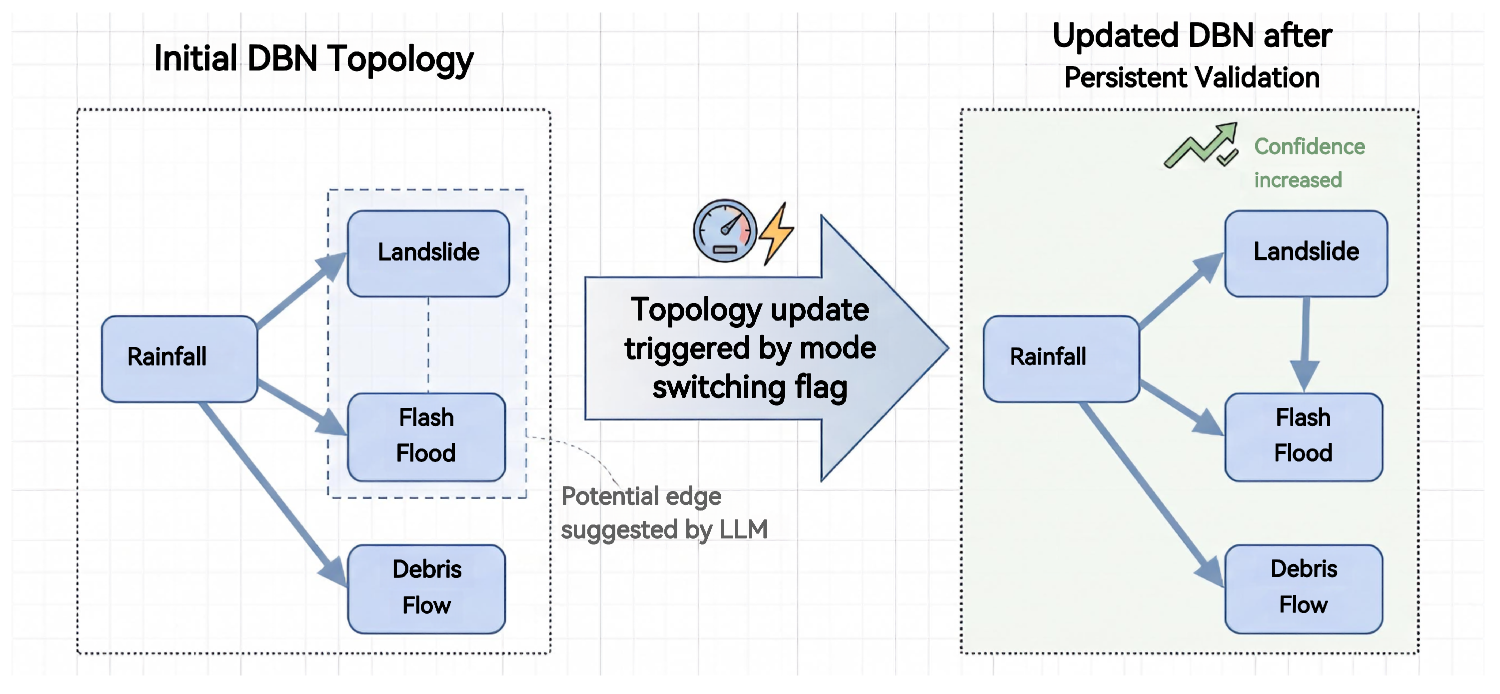
Taking the Xi’an 9.16 Rainstorm Disaster Chain as an example, the practical effect of dynamic DBN topology reconstruction is illustrated. The initial DBN was preconfigured with basic edges such as “rainfall → landslide,” “rainfall → flash flood,” and “rainfall → debris flow,” but did not include “landslide → flash flood.” In conventional understanding, flash floods are typically triggered directly by short-duration heavy rainfall; whether the landslide in this event influenced the subsequent flash flood formation required the LLM to identify through analysis of window data. On the day of the event, short-duration heavy rainfall intensified continuously from the morning onward. When parsing the window data at the fourth hour, the LLM captured the following anomalous signals: the hourly rainfall increase was significant, but channel hydrological monitoring data showed that the downstream water level rise was lower than the historical average under equivalent rainfall intensity. After comprehensive analysis, the LLM inferred that there was localized channel blockage, and the blocking material most likely originated from an upstream landslide or collapse, thus outputting “landslide → flash flood” as a potential causal edge suggestion. As window data continued to be input, the confidence level of the suggested edge gradually accumulated. By the ninth hour, the channel monitoring data exhibited an abrupt change, with the water level rising sharply within a short period, ultimately validating the blockage assessment from the preceding windows. The “landslide → flash flood” edge was formally activated, thereby expanding the DBN from a simple structure focusing only on “rainfall → flash flood” to a complete cascade reasoning network of “rainfall → landslide → flash flood”. The DBN topology reconstruction driven by LLM latent parameters is shown in Figure 4.

At the parameter level, during the dynamic evolution of rainstorm disaster chains, the CPT parameters of the DBN typically rely solely on frequency statistics from historical monitoring data. When data are sparse or the evolution phase switches, purely data-driven maximum likelihood estimation is prone to overfitting or delayed response to abrupt changes. The causal dependency strength ${\rho }_{ij}^{\left(t\right)}$ output by the LLM encapsulates domain prior knowledge within the current window context. By injecting it into Bayesian estimation in the form of pseudo-counts, an adaptive balance between data and prior can be achieved. The causal dependency strength ${\rho }_{ij}^{\left(t\right)}$ is injected into CPT learning as a prior. For the conditional probability of a state node j given that its parent node i is in the active state, a prior pseudo-count is introduced:

$${\alpha }_{j|i}^{\left(t\right)}={\alpha }_0·{\rho }_{ij}^{\left(t\right)}+{\alpha }_{min}$$

(6)

Here, the value of ${\alpha }_0$ is determined by the likelihood on the validation set; ${\alpha }_{min}=0.1$. The prior pseudo-counts are updated with ${\rho }_{ij}^{\left(t\right)}$ at each time slice and passed to the cascade verification stage. Specifically, a linear mapping is used to convert ${\rho }_{ij}^{\left(t\right)}\in [0,1]$ into pseudo-counts ${\alpha }_{j\mid i}^{\left(t\right)}\in [{\alpha }_{min}$,${\alpha }_0+{\alpha }_{min}]$, where ${\alpha }_0$ controls the relative weight of the prior: the larger ${\alpha }_0$, the stronger the influence of the LLM prior on the posterior estimate; ${\alpha }_{min}$ ensures that a weak prior is retained even when ${\rho }_{ij}^{\left(t\right)}=0$, thus avoiding the zero-probability problem. By selecting ${\alpha }_0$ through maximizing the log-likelihood on the validation set, the optimal fusion ratio between the prior and the data can be quantified without introducing subjective bias. This mechanism allows the CPT parameters to be updated with ${\rho }_{ij}^{\left(t\right)}$ at each time slice. When the disaster chain is in a stable phase, the model primarily trusts the observed data; when strong causal signals emerge during rapid evolution phases, the prior weight is automatically increased, thereby achieving instant injection of domain knowledge while maintaining statistical robustness, and providing more accurate probabilistic inputs for the subsequent cascade verification.

Still taking the Xi’an 9.16 rainstorm disaster chain as an example, in the early stage of the rainstorm, the cumulative rainfall was low, and the antecedent soil moisture had not yet reached saturation. After parsing the window data, the LLM output a causal dependency strength of ${\rho }_{rain,\mathrm{landslide}}^{\left(t\right)}\approx 0.18$ for “rainfall → landslide.” At this point, the prior pseudo-count was small, the CPT parameters of the landslide node were primarily driven by actual monitoring data, and the model’s posterior estimate of landslide probability remained at a low level. As the rainfall continued, the hourly rainfall gradually increased and the cumulative rainfall exceeded a critical threshold. The LLM detected the triggering of the pattern switching indicator ${\delta }_t$, and after re-evaluation, ${\rho }_{rain,\mathrm{landslide}}^{\left(t\right)}$ rose to 0.73, substantially increasing the prior pseudo-count and greatly boosting the prior probability of the landslide node under rainfall conditions. As a result, the DBN raised the landslide probability to the warning threshold well before the actual event.

2.

Feedback Optimization of Sliding Window Width and Step Size

The evolution of a disaster chain is a dynamically changing process, with different phases imposing different requirements on the window. For example, during a stable phase with sustained rainfall but no disaster triggering, a wider window should be used to capture macro trends and suppress noise; during a rapid evolution phase with sharply increasing rainfall intensity or imminent disaster occurrence, the window needs to be rapidly shortened to enhance sensitivity to abrupt change signals. To this end, this study utilizes the outputs of the perception–reasoning stage, ${\delta }_t$ and ${\tau }_k^{\left(t\right)}$, which are passed to the dynamic regulation stage. Based on Formulas (7) and (8), $L_{\max }$ and $H_t$ are sequentially updated. The updated parameters are then passed to the perception–reasoning stage at the next moment, where they are used to recalculate the window length $L_t$ and window content $W_t$. The new window data in turn drive the LLM parsing again, forming a positive reinforcement loop of “perception → regulation → re-perception.”

First, by adjusting the upper bound $L_{max}$ of the window length, the window calculation at the next moment can be influenced, thereby achieving the purpose of dynamically adjusting the sliding window size. The correction rule is as follows:

$$L_{max}^{\left(t\right)}=\left\{\begin{array}{cc}max(L_{min},L_{max}^{(t-1)}-\Delta L),\hfill & {\displaystyle \frac{\left|\{k\mid {\tau }_k^{\left(t\right)}\ne \mathrm{stable}\}\right|}{K}}\ge {\theta }_{\tau }\hfill \\ min(L_{max}^{\left(0\right)},L_{max}^{(t-1)}+\Delta L),\hfill & \forall k,{\tau }_k^{\left(t\right)}=\mathrm{stable}\hfill \\ L_{max}^{(t-1)},\hfill & \mathrm{otherwise}\hfill \end{array}\right.$$

(7)

where K denotes the number of disaster nodes (taken as 4 in this study), ${\theta }_{\tau }=0.5$, $\Delta L=1$ h, $L_{\max }=12$ h, and $L_{min}=2$ h. When the evolution trend of more than half of the nodes is non-stable (i.e., rising or declining), $L_{max}$ is reduced, thereby further compressing the window width on top of the exponential decay in Formula (3) to make the model more focused on rapidly changing periods. When all nodes are stable, $L_{max}$ gradually recovers to its initial value, and the window width increases accordingly.

Second, the adaptive update rule for the sliding step size $H_t$ is as follows:

$$\begin{array}{c}\hfill H_t=\left\{\begin{array}{cc}\max (H_{\min },H_{t-1}-\Delta H),\hfill & {\delta }_t=1\hfill \\ \min (H_{\max },H_{t-1}+\Delta H),\hfill & {\delta }_t=0\mathrm{and}\forall k,{\tau }_k^{\left(t\right)}=\mathrm{stable}\hfill \\ H_{t-1},\hfill & \mathrm{otherwise}\hfill \end{array}\right.\end{array}$$

(8)

Here, $H_{min}=1$, $H_{max}$ is set to one-quarter of the average duration of rainstorm events, and $\Delta H=1$ h. When the perception–reasoning stage detects a pattern switch (${\delta }_t=1$), the step size is immediately reduced so that the next window samples data from the rapid evolution phase more densely. When the evolution trends of all disaster nodes are stable (${\tau }_k^{\left(t\right)}=\mathrm{stable}$) and there is no pattern switch, the step size is gradually increased to reduce the computational burden during stable periods. In all other cases, the step size remains unchanged.

Regarding the concern that the adaptive window may expand to $L_{max}=12$ h during prolonged stable rainfall, potentially smoothing critical saturation signals: the model employs three complementary mechanisms that jointly prevent the loss of critical transition information. First, the cumulative rainfall $C_t$ is explicitly tracked as a monotonic input feature within every window regardless of its instantaneous length. Even in a 12 h window, the cumulative rainfall values at the tail hours faithfully reflect the total water input and the approach toward soil saturation, and the LLM directly analyzes $C_t$ trends alongside other multivariate signals in the structured text block $T_t$. Second, the pattern switching indicator ${\delta }_t$ is derived from the LLM’s holistic analysis of the full multivariate state vector—including $C_t$, hourly rainfall intensity $R_t$, and the disaster state vector—rather than depending solely on the inter-time-slice similarity $S_t$. When the LLM detects that $C_t$ is approaching critical thresholds learned from historical disaster events (e.g., the 85 typical events in the knowledge base), it can independently set ${\delta }_t=1$, triggering Formula (7) to compress $L_{max}$ and sharpen the window focus regardless of the $S_t$-based exponential decay. Third, the exponential decay mechanism of Formula (3) ensures that even during extended windows, recent observations at the tail of the window carry proportionally greater influence in the LLM’s context due to their temporal proximity to the prediction target. These mechanisms together ensure that the model does not miss soil saturation transitions, and the empirical results in Section 3 (MWLT = 4.6 h, recall = 83.0%) confirm that the adaptive window achieves effective early detection of disaster precursors.

2.2.5. Cascade Verification

After the perception–reasoning and dynamic regulation stages, the DBN topology $A_t$ and the prior pseudo-counts ${\alpha }_{j\mid i}^{\left(t\right)}$ that are adapted to the current evolution state have been obtained. This section constructs a dynamic Bayesian network based on the above inputs to perform probabilistic reasoning and model validation for the rainstorm disaster chain.

Let the time slice length be $\Delta t=1$ h. Within each time slice t, a static Bayesian network $B_t$ is constructed. The DBN node set consists of state nodes $S_t$ (landslide, debris flow, flash flood, waterlogging, with binary states) and evidence nodes $E_t$. The evidence nodes are divided into two categories: temporally driven evidence, which serves as exogenous input; and spatial background evidence, which is treated as static nodes and assigned values only in the initial time slice. The causal dependencies within the same time slice are determined by the active edge set $A_t$ output from the dynamic regulation stage. Different time slices are connected through the state transition network $B_{\to }$, where the conditional probability of a state node at time t + 1 depends on the evidence nodes within the same time slice and the state nodes in the previous time slice that have causal associations with it. The joint probability distribution of the entire DBN is decomposed as follows:

$$P\left(X_{1:T}\right)={\displaystyle \prod _{t=1}^T}\prod _{X\in X_t}P(X\mid \mathrm{Pa}\left(X\right))$$

(9)

where Pa(X) denotes the set of parent nodes of node X, and parent nodes can come from the same time slice or the previous time slice.

CPT parameters are estimated using Bayesian estimation, with ${\rho }_{ij}^{\left(t\right)}$ output from the dynamic regulation stage injected as a prior. For the conditional probability of state node j given its parent configuration ${\mathbf{pa}}_j$, using the prior pseudo-counts ${\alpha }_{j\mid i}^{\left(t\right)}$, the maximum a posteriori estimate is

$${\widehat{\theta }}_{j|{\mathbf{pa}}_j}^{\left(t\right)}={\displaystyle \frac{N_{j|{\mathbf{pa}}_j}+{\alpha }_{j|i}^{\left(t\right)}}{M_{j|{\mathbf{pa}}_j}+2{\alpha }_{j|i}^{\left(t\right)}}}$$

(10)

This estimate relies on data frequencies when samples are sufficient, and shrinks toward the LLM prior when they are sparse.

After completing the DBN construction and parameter estimation, real-time monitoring data within the current window are input as evidence, and exact inference is performed using the junction tree algorithm to output the dynamic prediction results of the disaster chain. The inference process mainly includes: evidence input (observed values from the current time slice), forward propagation (computing the posterior probabilities of each state node for the next h hours), warning determination (issuing a warning when the posterior probability exceeds the threshold ${\theta }_{warn}=0.5$), and chain path tracing (tracing back along the directed edges of the DBN to identify the complete causal chain from hazard factors to disaster consequences). Model validation adopts an event-wise chronological split (detailed in Section 3.1): rainstorm events are assigned to training, validation, and test sets by their occurrence dates without fragmentation, ensuring temporal isolation and preventing information leakage across splits. The training set is used for CPT learning, the validation set for threshold and hyperparameter calibration, and the test set for evaluating the model’s prediction accuracy and early warning timeliness. Compared with traditional static BNs or fixed-structure DBNs, the network structure of the proposed model is driven in real time by LLM latent parameters, the CPT parameters integrate semantic priors, and the inference results feature both probabilistic quantification and causal interpretability. For a complete overview of all key parameters used in the SW-DBN model, please refer to

Table A1. Key parameters and hyperparameters of the SW-DBN model.

Parameter Name	Symbol	Value	Description
Minimum window length	$L_{\min }$	2 h	Adaptive window lower bound
Initial maximum window length	$L_{\max }^{\left(0\right)}$	12 h	Adaptive window initial upper bound
Decay coefficient	$\lambda$	Calibrated by historical events	Window sensitivity to change intensity
Minimum sliding step	$H_{\min }$	1 h	Sliding step lower bound
Maximum sliding step	$H_{\max }$	4 h	≈1/4 of avg. rainstorm duration, rounded to integer
Step adjustment	$\Delta H$	1 h	Per-step adjustment
Window upper bound adjustment	$\Delta L$	1 h	$L_{\max }$ per-update adjustment
Unstable trend threshold	${\theta }_{\tau }$	0.5	Trigger $L_{\max }$ compression threshold
DBN edge activation threshold	${\theta }_{\rho }$	Determined on validation set	Causal edge activation threshold
Confidence counter confirmation period	$T_{\mathrm{confirm}}$	9 h	Confirmation time window
Confidence counter confirmation times	$N_{\mathrm{confirm}}$	3	Required confirmation counts
Confidence counter expiration period	$T_{\mathrm{expire}}$	18 h	Expiration time window
CPT prior pseudo-count coefficient	${\alpha }_0$	Maximized log-likelihood on validation set	LLM prior weight coefficient
Minimum CPT prior pseudo-count	${\alpha }_{\min }$	0.1	Prevent zero-probability
Early warning threshold	${\theta }_{\mathrm{warn}}$	0.5	Posterior probability warning threshold

in Appendix A.

3. Results

3.1. Experimental Environment

(1)

The experimental hardware configuration is detailed in

Table 1. Experimental hardware configuration.

Item	Model/Specification
CPU	Intel Xeon Silver 4216 × 2
Memory	64 GB RAM
GPU	NVIDIA GeForce RTX 3090
Storage	1 TB NVMe SSD

.

(2)

The core software environment used in this experiment is detailed in

Table 2. Experimental software environment.

Software Name	Version
Ubuntu Server	22.04
Python	3.13.12
PyTorch	2.9.0
DeepSeek	R1-14B
PostgreSQL/PostGIS	15.14/3.6

.

3.2. Evaluation Metrics

To comprehensively evaluate the performance of the SW-DBN model in the dynamic prediction of rainstorm disaster chains, this paper constructs an evaluation index system from two dimensions: prediction accuracy and early warning timeliness.

3.2.1. Prediction Accuracy Metrics

For the prediction of occurrence probabilities of key disaster nodes such as landslides, debris flows, flash floods, and waterlogging, the posterior probabilities output by the model are compared with the actual disaster occurrence states. Let the total number of test samples be N, with actual disaster occurrences regarded as positive examples and non-occurrences as negative examples. The model’s prediction results are categorized into: true positive (TP), false positive (FP), true negative (TN), and false negative (FN). The following metrics are defined:

(1)

Accuracy (ACC)

$$ACC={\displaystyle \frac{TP+\mathrm{TN}}{N}}$$

(11)

Accuracy measures the model’s overall discriminative ability for all samples. In this paper, the average accuracy across the four nodes—landslide, debris flow, flash flood, and waterlogging—is used as the final accuracy.

(2)

Precision (P)

$$P={\displaystyle \frac{\mathrm{TP}}{TP+FP}}$$

(12)

Precision reflects the proportion of samples predicted by the model as disaster occurrences that actually occurred, indicating the reliability of the prediction results.

(3)

Recall (R)

$$R={\displaystyle \frac{\mathrm{TP}}{TP+FN}}$$

(13)

Recall measures the model’s ability to capture actual disaster events, reflecting the risk of missed alarms.

(4)

F1-Score (F1)

$$F1=2\times {\displaystyle \frac{P\times R}{P+R}}$$

(14)

The F1-score is the harmonic mean of precision and recall, providing a comprehensive evaluation of the model’s predictive balance.

(5)

AUC-ROC The area under the receiver operating characteristic curve (AUC-ROC) is adopted as an overall performance metric independent of threshold selection. An AUC value closer to 1 indicates a stronger ability of the model to distinguish between disaster occurrence and non-occurrence.

3.2.2. Early Warning Timeliness Metrics

The core value of rainstorm disaster chain prediction lies in issuing early warnings in advance to buy time for emergency response. This paper introduces the mean warning lead time (MWLT) to evaluate the model’s early warning timeliness.

For the i-th actual disaster event, let $t_{warn,i}$ be the moment when the model first raises the disaster occurrence probability to the threshold $\theta =0.5$, and $t_{occur,i}$ be the moment when the disaster actually occurs. The warning lead time is then

$$\Delta t_i=t_{\mathrm{occur},i}-t_{\mathrm{warn},i}$$

(15)

The mean over all test events is then taken as

$$MWLT={\displaystyle \frac{1}{M}}{\displaystyle \sum _{i=1}^M}\Delta t_i$$

(16)

where M is the total number of actual disaster events in the test set. The unit of MWLT is hours, and a larger value indicates more timely warnings from the model.

To ensure the fairness of comparison results across different models, this study applies consistent data partitioning, input features, prediction targets, and evaluation metrics to all models.

Experimental samples are constructed with a time step of 1 h, with inputs being the multi-source observation data within the current sliding window, and the prediction targets being the occurrence probabilities of the four types of state nodes—landslide, debris flow, flash flood, and urban waterlogging—over the next n hours.

Considering the pronounced temporal continuity of rainstorm disaster chains and the need to prevent temporal leakage in early-warning tasks, this study adopts an event-wise chronological split over a study period spanning two decades (2007–2026). The samples are partitioned by complete rainstorm event boundaries into training, validation, and test sets in proportions of approximately 70%, 15%, and 15%, respectively. Specifically, the training set covers January 2007 to December 2020, the validation set covers January 2021 to December 2023, and the test set covers January 2024 to December 2026. Each split contains complete rainstorm events without fragmentation, and no event spans across split boundaries. For the pre-July 2025 period, coarser district/county-level rainfall data are used; from July 2025 onward, high-density station-level rainfall records are available. The positive/negative sample counts per disaster node in each split are reported in

Table 3. Data split statistics: date ranges and per-node positive/negative sample counts.

Split	Date Range	Landslide (Pos/Neg)	Debris Flow (Pos/Neg)	Flash Flood (Pos/Neg)	Waterlogging (Pos/Neg)
Train	2007–2020	152/7600	7/350	346/17,300	95/4750
Validation	2021–2023	33/1650	1/50	75/3750	21/1050
Test	2024–2026	33/1650	1/50	75/3750	21/1050

. All LLM prompts, knowledge base retrievals, and latent parameter extractions are restricted to using only information from the training period and earlier, with strict temporal isolation from validation and test periods.

The training set is used for model parameter learning, the validation set for threshold selection and prior weight calibration, and the test set exclusively for final performance evaluation. To prevent information leakage from the test period into the LLM’s reasoning process, strict temporal isolation is enforced. The disaster knowledge base used for LLM prompt construction contains only historical disaster reports and event records whose occurrence dates precede the start of the test period. Any disaster report, news article, or structured record with a timestamp later than the validation period’s end date is excluded from the knowledge base. The LLM prompt template references only the multi-source observations within the current sliding window and the temporally isolated knowledge base; no future or test-period outcomes are included. For the sliding window mechanism, the window at any time t uses only observations up to time t, and the LLM’s causal inference is based exclusively on patterns visible within this backward-looking window. This temporal isolation protocol ensures that the LLM cannot “peek” into the test period when generating latent parameters, thereby guaranteeing a realistic evaluation of the model’s predictive capability. For SW-DBN, the activation threshold, upper and lower bounds of the window length, sliding step size, and CPT prior pseudo-count weights are all determined on the validation set and kept fixed during the testing phase.

It should be noted that MWLT is calculated only for models with temporal prediction capability. Since a static BN lacks a temporal transition structure and cannot output rolling updated warning lead times, its MWLT is denoted as N/A.

3.3. Comparative Experiments

To comprehensively evaluate the performance of the proposed SW-DBN model in the dynamic prediction of rainstorm-induced disaster chains, this paper conducts comparative experiments against seven representative baseline models (static BN, standard DBN, LSTM, RF, TCN, transformer, and CP-DBN) on the Xi’an study area dataset under identical training, validation, and test set partitions. All models adopt consistent input features, prediction time scales, and evaluation metrics to ensure the comparability of experimental results. The selected comparison models span traditional static risk assessment, dynamic probabilistic graphical models, classical machine learning methods, and deep learning temporal prediction models, specifically including

• Static Bayesian Network (Static BN): Represents the traditional static risk assessment method, where the network structure and parameters do not evolve over time.
• Standard Dynamic Bayesian Network (Standard DBN): Serves as the baseline method for dynamic probabilistic graphical models, with a network structure adopting a predefined chain topology and parameters learned solely from monitoring data through maximum likelihood estimation, without incorporating any external knowledge or feature optimization strategies.
• Long Short-Term Memory Network (LSTM): A classical variant of recurrent neural networks adept at capturing temporal dependencies. This paper constructs a two-layer LSTM network, with the input being the multivariate time-series sequence within the sliding window and the output being the occurrence probabilities of the four disaster nodes—landslide, debris flow, flash flood, and waterlogging—for the next hour. The hidden layer dimension is set to 128, with Dropout (0.2) applied to prevent overfitting.
• Random Forest (RF): A classical ensemble learning model widely used in disaster risk assessment. To adapt to the temporal prediction task, dynamic monitoring data such as meteorological and hydrological variables from the past 24 h are concatenated with static environmental factors as a feature vector to directly predict the disaster occurrence state. The Random Forest contains 200 decision trees with a maximum depth of 15.
• Temporal Convolutional Network (TCN): A non-recurrent temporal model using dilated causal convolutions to capture long-range dependencies. The TCN is configured with 4 residual blocks; a kernel size of 3; and dilation rates of 1, 2, 4, 8, and 128 hidden channels trained with the same input window and prediction horizon as LSTM.
• Transformer: A self-attention-based temporal model. The transformer encoder is configured with 4 attention heads, 2 layers, a feed-forward dimension of 512, and positional encoding for the temporal dimension. It takes the same multivariate time-series input as LSTM and TCN.
• Adaptive DBN with Statistical Change Point Detection (CP-DBN): A non-LLM adaptive DBN baseline where the pattern switching indicator ${\delta }_t$ is derived from a CUSUM (cumulative sum) change point detection algorithm applied to the rainfall intensity time series, instead of the LLM. The DBN topology is adjusted using the same candidate edge set, but causal strengths are computed from purely data-driven correlation coefficients rather than LLM priors. This baseline isolates the contribution of the LLM component by replacing it with a statistical alternative.
• SW-DBN: The complete SW-DBN model proposed in this paper.

To ensure fair comparison, all baseline models underwent systematic hyperparameter optimization using the same validation protocol. For the standard DBN, the number of time slices was tuned over 2, 3, 4, 6, 8, 12 and the structure learning algorithm compared between hill-climbing and Tabu Search. For LSTM, a grid search was conducted over hidden layer dimensions 64, 128, 256, number of layers 1, 2, 3, dropout rates 0.1, 0.2, 0.3, 0.5, learning rates ${10}^{-3}$, $5\times {10}^{-4}$, ${10}^{-4}$, and batch sizes 32, 64, 128, with early stopping (patience = 10) on validation loss. For Random Forest, the number of trees was tuned over 100, 200, 300, 500, maximum depth over 10, 15, 20, None, and minimum samples per split over 2, 5, 10, using 5-fold time-series cross-validation on the training set. For TCN, the kernel size was tuned over 2, 3, 5, the number of residual blocks over 2, 3, 4, 6, hidden channels over 64, 128, 256, dropout over 0.1, 0.2, and learning rate over ${10}^{-3}$, $5\times {10}^{-4}$, ${10}^{-4}$, with early stopping (patience = 10). For transformer, the number of attention heads was tuned over 2, 4, 8, encoder layers over 1, 2, 3, 4, feed-forward dimension over 256, 512, 1024, dropout over 0.1, 0.2, 0.3, and learning rate over ${10}^{-3}$, $5\times {10}^{-4}$, ${10}^{-4}$, also with early stopping. For CP-DBN, the CUSUM detection threshold was tuned over 0.5, 1.0, 1.5, 2.0 standard deviations and the detection window length over 3, 6, 9, 12 h, with the correlation method compared between Pearson and Spearman correlations for computing data-driven causal strengths. All hyperparameter selections were finalized on the validation set and kept fixed during test set evaluation. To address class imbalance, LSTM, RF, TCN, and transformer all employed weighted loss functions (inverse class frequency) computed from the training set only. Random seeds were fixed at 42 for all models to ensure reproducibility.

All model input features undergo the same standardization processing, with normalization parameters for continuous variables computed solely from the training set and applied to the validation and test sets. All models are evaluated on the same test set, and the experimental results are detailed in

Table 4. Performance comparison of different models for rainstorm disaster chain prediction in the Xi’an study area.

Model	ACC, %	P, %	R, %	F1-Score, %	AUC-ROC	MWLT, Hour
Static BN	68.2	65.1	60.3	62.6	0.71	N/A
Standard DBN	77.3	74.5	72.8	73.6	0.83	2.8
LSTM	79.8	77.2	76.5	76.8	0.86	2.4
RF	75.6	73.8	71.2	72.5	0.80	1.9
TCN	81.2	79.5	80.8	80.1	0.87	2.5
Transformer	82.4	80.8	81.5	81.1	0.88	2.7
CP-DBN	80.5	78.2	79.0	78.6	0.85	3.5
SW-DBN	84.8	83.5	83.0	83.3	0.89	4.6

.

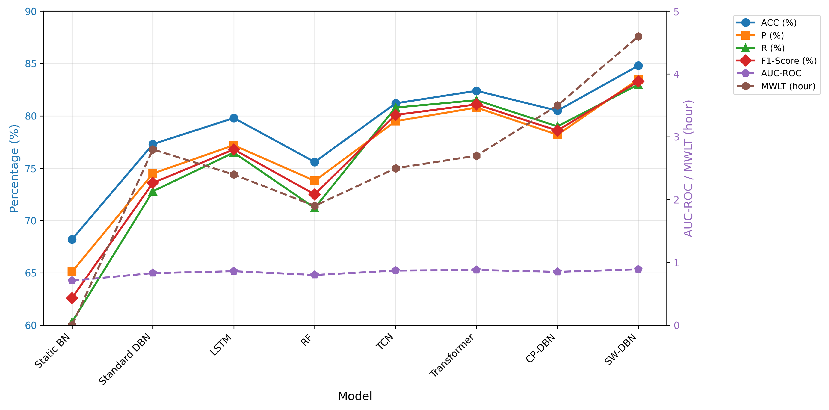
As can be seen from Table 4, the static BN performed the worst across all metrics (accuracy 68.2%, AUC-ROC only 0.71), confirming the fundamental deficiency of static methods in characterizing the temporal evolution of disaster chains. After introducing time slices and a state transition mechanism, the standard DBN achieved an accuracy improvement to 77.3% and an MWLT of 2.8 h, indicating that dynamic modeling provides a significant gain for rainstorm disaster chain prediction. As a purely data-driven model, LSTM outperformed the standard DBN in accuracy (79.8%) and AUC-ROC (0.86), but its MWLT was only 2.4 h, lower than that of the standard DBN. This is because LSTM is insensitive to early weak signals, often leading to a sharp probability rise only when a disaster is imminent, resulting in a smaller warning lead time, whereas the DBN, relying on the causal graph structure, can gradually increase probabilities in advance based on physical mechanisms. The TCN and Transformer models achieved accuracies of 81.2% and 82.4%, respectively, demonstrating the advantages of deep temporal architectures over classical machine learning for capturing nonlinear dependency patterns. However, as purely data-driven models without causal priors, their MWLT values (2.5 h and 2.7 h) remained below that of SW-DBN, consistent with the LSTM observation that black-box models tend to react only at the late stage of disaster evolution. The CP-DBN, which replaces the LLM component with statistical CUSUM change point detection, achieved an accuracy of 80.5% and an MWLT of 3.5 h. The 4.3 percentage point accuracy gap between CP-DBN and SW-DBN quantifies the net contribution of the LLM-driven semantic reasoning over purely statistical alternatives, while the 1.1 h MWLT improvement confirms that LLM priors enable earlier detection of disaster precursors.The overall performance of the RF model ranked only above the static BN among the baseline models, with an accuracy of 75.6% and an MWLT of merely 1.9 h, indicating that conventional machine learning methods struggle to adequately capture the high-dimensional temporal dependencies of disaster chains.

The proposed SW-DBN model achieved the best results across all evaluation metrics: accuracy reached 84.8%, an improvement of 7.5 percentage points over the standard DBN; recall reached 83.0%, demonstrating the model’s strong capability to capture actual disaster events; the F1-score was 83.3%, indicating a good balance between precision and recall; AUC-ROC reached 0.89, showing the strongest ability to distinguish between disaster occurrence and non-occurrence; and MWLT reached 4.6 h, representing an improvement of 1.8 h and 2.2 h over the standard DBN and LSTM, respectively, demonstrating a clear advantage in early warning timeliness. These advantages are attributable to the closed-loop framework of “perception–reasoning, dynamic regulation, and cascade verification”: the adaptive sliding window focuses on critical evolution phases, the LLM latent parameters inject causal structural priors into the DBN, the dynamic regulation mechanism enables adaptive updating of the topology and window parameters, and the framework ultimately outputs chain prediction results that combine high accuracy with interpretability. To provide a more granular assessment,

Table 5. Per-node performance of SW-DBN with bootstrap 95% confidence intervals.

Node	Precision	Recall	F1	AUC	FAR (%)	MAR (%)	MWLT (h)
Landslide	85.2	84.5	84.8	0.91	12.3	15.5	5.2
Debris flow	82.8	81.2	82.0	0.88	14.0	18.8	4.8
Flash flood	83.5	82.0	82.7	0.89	13.2	18.0	4.2
Waterlogging	84.5	85.0	84.7	0.90	15.5	15.0	4.0
Macro Avg	84.0	83.2	83.6	0.90	13.8	16.8	4.6
Overall ACC	84.8% (95% CI: 82.1–87.5%)
Overall AUC	0.89 (95% CI: 0.86–0.92)

reports the per-node precision, recall, F1, AUC, false alarm rate (FAR), missed alarm rate (MAR), and MWLT for the SW-DBN model on the test set. FAR is defined as FP/(FP+TN) and MAR as FN/(TP+FN). Bootstrap 95% confidence intervals (1000 resamples) are reported for overall ACC and AUC. Statistical significance of the SW-DBN’s improvement over the strongest baseline (transformer) was assessed using McNemar’s test for per-node classification outcomes and DeLong’s test for AUC comparisons. McNemar’s test was applied to the hourly binary predictions on the test set (total of 21,890 samples), yielding $p=0.003$, indicating a statistically significant improvement at the $(\alpha =0.01)$ level. DeLong’s test gave $p=0.008$, confirming that the AUC gain is not due to chance.

A radar chart comparing the performance of each model is shown in Figure 5.

3.4. LLM Output Quality Evaluation

To validate the reliability of the LLM-derived latent parameters, an independent evaluation was conducted by comparing the LLM outputs against expert-labeled causal chains from 85 historically verified disaster events [9]. Three domain experts in geological hazards and hydrology independently labeled the causal relationships (pattern switching moments, causal edge strengths, and evolution trends) for a subset of 20 representative events drawn from the training period. The LLM was then prompted with the same multi-source window data for these events (using identical prompt settings, decoding parameters, and JSON validation rules as in the main experiments), and its outputs were compared against the expert consensus labels.

Table 6. LLM output quality evaluation against expert-labeled chains.

Output Type	Accuracy/Agreement	Precision	Recall	F1
Pattern switching (${\delta }_t$)	0.87	0.84	0.82	0.83
Causal strength (${\rho }_{ij}$) MAE	0.12	-	-	-
Evolution trend (${\tau }_k$)	0.82	0.79	0.76	0.77
Causal edge suggestions	0.76	0.72	0.69	0.70

Note: “-” indicates that the metric is not applicable for this output type. For causal strength (${\rho }_{ij}$), only the mean absolute error (MAE) is reported because it is a continuous error metric, not a classification metric; therefore, precision, recall, and F1 are not defined.

summarizes the evaluation results.

The results show that the LLM achieved 87% agreement with experts on pattern switching detection (${\delta }_t$), with F1 = 0.83, demonstrating reliable identification of phase transitions in the rainstorm disaster chain. Causal strength estimation (${\rho }_{ij}$) showed a mean absolute error of only 0.12 on the $[0,1]$ scale, confirming that the five-level ordinal rubric produces numerically well-calibrated outputs. Evolution trend prediction (${\tau }_k$) reached 82% accuracy (F1 = 0.77), with most errors occurring at trend inflection points where even experts showed disagreement. Causal edge suggestions exhibited the lowest agreement (76%, F1 = 0.70), with the primary error sources being rare disaster chain patterns not well represented in the knowledge base (e.g., compound chains involving infrastructure cascades) and ambiguous terminology in unstructured reports. The two false-positive edge suggestions were both filtered out by the persistence validation mechanism before reaching the DBN structure. These results confirm that the LLM-derived parameters, when constrained by the formalized pipeline described in Section 2.2.3, produce outputs that are broadly consistent with domain expert judgment, with the persistence validation providing an additional safety layer for the noisiest output type.

3.5. Ablation Experiments

To quantitatively evaluate the individual contributions of each core module in the SW-DBN model and further verify the sources of performance improvement, this paper designs ablation experiments under the same data partitioning, input features, and evaluation metrics as the comparative experiments. All models are based on the same DBN architecture, with the following variants constructed by retaining or removing specific modules:

(1)

Baseline: Standard DBN without any optimization modules.

(2)

Model A: Baseline + adaptive sliding window, DBN structure remains static.

(3)

Model B: Baseline + LLM latent parameters, fixed window.

(4)

Model C: Baseline + sliding window + LLM latent parameters, dynamic regulation disabled.

(5)

Model D: The complete SW-DBN model proposed in this paper.

The experimental results are shown in

Table 7. Ablation experiment results of the SW-DBN model on the Xi’an study area.

Model	ACC, %	P, %	R, %	F1-Score, %	AUC-ROC	MWLT, Hour
Baseline	77.3	74.5	72.8	73.6	0.83	2.8
Model A	80.1	77.8	78.5	78.1	0.85	3.8
Model B	82.1	80.2	79.5	79.8	0.87	3.9
Model C	83.8	82.5	81.9	82.2	0.88	4.3
Model D	84.8	83.5	83.0	83.3	0.89	4.6

.

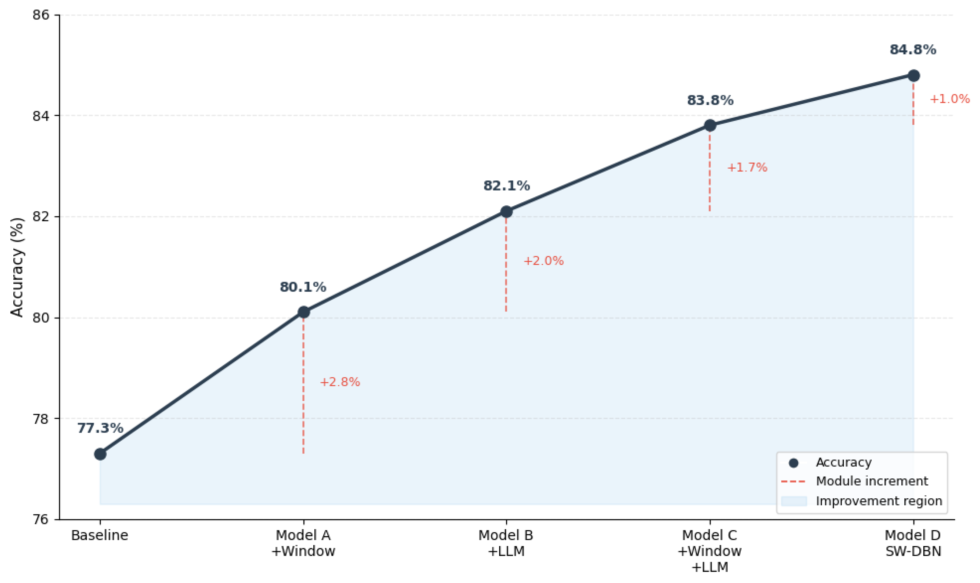
As shown in Table 7, the introduction of any single module yielded significant improvements. Compared to the baseline, Model A (with the adaptive sliding window) improved accuracy by 2.8 percentage points, recall by 5.7 percentage points, and MWLT by 1.0 h. AUC-ROC was increased from 0.83 to 0.85, verifying the improvement in early perception capability brought by the dynamic window. Model B (with LLM latent parameter mining) improved accuracy by 4.8 percentage points, extended MWLT by 1.1 h, and raised AUC-ROC to 0.87, indicating that the LLM causal prior contributes most significantly to improving the model’s predictive logic. Model C (with both the sliding window and LLM latent parameters, but without dynamic regulation) further improved accuracy by 1.7 percentage points over Model B, with AUC-ROC rising to 0.88, reflecting the synergistic effect of the sliding window and the LLM; however, without dynamic regulation, the latent parameters could not be adaptively updated along with the evolution. Model D (the complete SW-DBN) further introduced the dynamic regulation mechanism on top of Model C, improving accuracy by 1.0 percentage point (from 83.8% to 84.8%), AUC-ROC from 0.88 to 0.89, and MWLT by 0.3 h (from 4.3 to 4.6 h). Using the latent parameters inferred by the LLM, the dynamic regulation mechanism reconstructs the DBN topology online, updates CPT parameters in real time, and optimizes the window parameters via feedback. This enables the model to adaptively match the phased evolution of the disaster chain, resulting in a further performance leap over Model C. The contribution trends of each module to the model performance are illustrated in Figure 6.

3.6. Sensitivity Analysis of Sliding Window Parameters

The adaptive sliding window is a central component of the proposed SW-DBN model, and its behavior is governed by three key parameters: the minimum window length $L_{min}$, the initial maximum window length $L_{max}^{\left(0\right)}$, and the decay coefficient $\lambda$ (see Formula (3)). To quantify how these parameters influence prediction performance and warning lead time, a sensitivity analysis was conducted by varying each parameter independently while holding the others at their default values.

Table 8. Sensitivity analysis of sliding window parameters.

Parameter	Value	ACC (%)	MWLT (Hour)
$L_{min}$ (h)	1	83.2	4.1
	2 (default)	84.8	4.6
	3	84.3	4.4
	4	82.5	3.8
$L_{max}^{\left(0\right)}$ (h)	6	81.8	3.5
	8	83.4	4.0
	10	84.2	4.4
	12 (default)	84.8	4.6
	16	84.5	4.3
$\lambda$	0.1	82.4	3.2
	0.3	83.9	4.1
	0.5 (default)	84.8	4.6
	0.7	84.3	4.9
	1.0	83.6	4.6

reports the sensitivity of ACC and MWLT to variations in $L_{min}$, $L_{max}^{\left(0\right)}$, and $\lambda$.

The results reveal three key patterns. First, ACC remains stable within $L_{min}\in [1,3]$ (83.2–84.8%) but degrades noticeably at $L_{min}=4$ (82.5%), confirming that an overly wide minimum window smooths out critical abrupt change signals during disaster triggering phases. Second, $L_{max}^{\left(0\right)}$ exhibits a concave relationship with performance: values below 10 h restrict the window’s ability to capture complete rainstorm evolution cycles (ACC 81.8% at 6 h), while excessive values (16 h) only marginally degrade MWLT (from 4.6 to 4.3 h) due to the adaptive contraction mechanism. Third, MWLT is most sensitive to $\lambda$, peaking at 4.9 h when $\lambda =0.7$ (faster window contraction), but with a 0.5 percentage point ACC penalty relative to the default $\lambda =0.5$, indicating a precision–timeliness trade-off. These findings confirm that the default parameter values selected from historical event statistics represent a reasonable trade-off between predictive accuracy and warning lead time, and that the adaptive nature of the window mechanism provides robustness against moderate parameter misspecification.

4. Discussion

The performance advantages of the SW-DBN model can be attributed to the synergistic effect of its three core modules.

The adaptive sliding window dynamically couples the window length with the evolution rhythm of the disaster chain, avoiding the information redundancy of a fixed window during stable periods and the response lag during abrupt change periods, thereby enabling the model to capture precursor signals of disaster triggering earlier.

The contribution of LLM-based latent parameter mining is the most significant. By parsing multi-source data patterns within the window, the LLM extracts four types of latent parameters—pattern switching indicators, causal dependency strengths, evolution trend estimates, and potential causal edge suggestions—thereby injecting domain knowledge of disaster chains into the probabilistic graphical model in a computable form. Among them, the persistent discovery mechanism for potential causal edges endows the model with the capability to autonomously learn new causal associations, which is difficult to achieve with traditional DBNs and purely data-driven models.

The dynamic regulation mechanism is the key to achieving a holistic leap in performance. By using the latent parameters output by the LLM to reconstruct the DBN topology online, revise CPT parameters in real time, and feed back to optimize window parameters, the model maintains structural adaptation and parameter stability during phase transitions in the evolution of the disaster chain. Ablation experiments show that the introduction of dynamic regulation further improves prediction accuracy and early warning timeliness on the basis of the synergy between the sliding window and the LLM, verifying the core value of the closed-loop feedback mechanism.

Significant synergistic reinforcement exists among the three modules: the sliding window provides high-quality context units for the LLM, the LLM’s latent parameters provide decision-making grounds for dynamic regulation, and dynamic regulation in turn optimizes the next round of window perception, forming a positive reinforcement loop of “perception–reasoning, dynamic regulation, and cascade verification.”

The SW-DBN model outputs time-varying probabilistic predictions and causal chain paths for rainstorm disaster chains, which can be naturally integrated with automatic control systems for urban drainage and sewer networks. For instance, the model’s node-level posterior probabilities (e.g., the waterlogging probability exceeding ${\theta }_{warn}=0.5$) can serve as trigger signals for real-time control of pumping stations, sluice gates, and storage tanks. The MWLT metric, which quantifies the time between warning issuance and disaster occurrence, directly informs the feasible time window for control actions. Furthermore, the causal chain tracing capability of the DBN allows operators to identify which upstream disaster nodes (e.g., flash flood, debris flow) are most likely to propagate into urban waterlogging, enabling targeted preventive interventions such as pre-emptive drainage or traffic diversion. Control-oriented approaches for mitigating combined sewer overflows, such as finite-state machine control optimized by simulated annealing [26], provide relevant frameworks for translating probabilistic disaster-chain predictions into operational decision rules. Future work may explore the coupling of SW-DBN output with model predictive control for sewer networks, forming a closed-loop “predict–control–feedback” system for urban flood resilience.

Although the LLM component functions as a semantic reasoning module whose internal representations are not fully transparent, the proposed SW-DBN framework provides multiple mechanisms for emergency-management users to trace, verify, and trust the model’s causal explanations. First, every LLM-derived parameter is accompanied by a structured reasoning trace in the prompt output: for each causal edge suggestion, the LLM is required to cite specific data evidence (e.g., sensor readings, rainfall anomaly patterns) from the current window, enabling human experts to audit the justification. Second, the DBN’s graphical structure itself serves as an interpretable white-box interface: once the LLM parameters are injected, all subsequent probabilistic reasoning follows well-defined Bayesian rules on an explicit causal graph, and the inference results are fully decomposable along the directed edges. Third, the chain path tracing mechanism (Section 2.2.5) allows users to backtrack from a predicted disaster consequence to its root hazard factors step-by-step, producing human-readable causal chains such as “rainfall → landslide → debris flow.” Fourth, the persistence validation mechanism for new causal edges ensures that only LLM suggestions consistently supported across multiple consecutive time windows are incorporated, reducing the risk of acting on transient model hallucinations. Together, these design choices transform the LLM from an opaque black box into an auditable parameter generator embedded within a transparent probabilistic graphical reasoning framework.

Regarding the choice of baseline models in the comparative experiments, we acknowledge that spatio-temporal graph neural networks such as spatio-temporal graph convolutional network (STGCN) and Graph WaveNet represent a valuable direction for benchmarking, as they can jointly model spatial topology (river networks, road networks) and temporal dynamics. The current comparative experiment was designed as a multi-paradigm evaluation spanning static assessment (static BN), dynamic probabilistic graphical models (standard DBN), classical machine learning (RF), deep temporal architectures (LSTM, TCN, transformer), and statistical change point detection (CP-DBN), with the goal of isolating the contributions of causal modeling and LLM-driven semantic reasoning. We recognize that STGCN and Graph WaveNet, which natively capture spatial correlations in graph-structured time series, could provide a more challenging benchmark for the spatial-topology aspect of disaster chain prediction. However, constructing a spatial adjacency graph from the river/road topology of the Xi’an area is a non-trivial task requiring careful engineering of graph edge definitions, and these models do not natively model the causal dependency structure among disaster nodes (e.g., landslide → debris flow) that is central to our framework. Incorporating STGCN and Graph WaveNet as baselines, along with the necessary spatial graph construction, is planned as a dedicated future work.

This study still has the following limitations. First, the reliability of LLM parsing highly depends on the design of prompts and the completeness of the disaster knowledge base, which may lead to misjudgments under rare disaster chain patterns or non-standard terminology descriptions. Future work may explore domain ontologies and retrieval-augmented generation methods to improve robustness. Second, some thresholds (such as the activation threshold, upper and lower bounds of window parameters, and confidence counter periods) are set based on statistics of historical events, and their applicability needs to be further verified when extreme events exceed the range of historical distributions. Third, the discretization of continuous variables in the DBN may introduce information loss, and future work may consider hybrid DBNs or continuous-node modeling.

5. Conclusions

This study proposes a dynamic prediction model for rainstorm disaster chains, SW-DBN, which integrates a large language model (LLM)-optimized sliding window mechanism with a dynamic Bayesian network (DBN). The model operates along a three-stage closed-loop pathway of “perception–reasoning, dynamic regulation, and cascade verification.” In the perception–reasoning stage, multi-source time-series data are segmented through an adaptive sliding window, and the LLM is invoked to mine four types of latent parameters: pattern switching indicators, causal dependency strengths, evolution trend estimates, and potential causal edge suggestions. In the dynamic regulation stage, these latent parameters are used to perform bidirectional adaptive adjustment—on the DBN side, the network topology is reconstructed and the conditional probability table parameters are updated; on the window side, the window width and step size are feedback-optimized. In the cascade verification stage, probabilistic reasoning is conducted based on the adjusted DBN, outputting posterior probabilities of disaster nodes and chain propagation paths. Experiments with the Xi’an area as the study region show that:

• The SW-DBN model achieves leading performance in the dynamic prediction of rainstorm disaster chains, with an average accuracy of 84.8% across four disaster nodes—representing improvements of 7.5, 2.4, and 4.3 percentage points over the standard DBN, transformer, and CP-DBN, respectively. Its MWLT of 4.6 h exceeds the best non-LLM baseline (CP-DBN: 3.5 h) by 1.1 h, and more than doubles that of LSTM (2.4 h). Per-node evaluation with bootstrap 95% confidence intervals and McNemar’s test ($p=0.003$) confirms that these gains are statistically significant. The LLM output evaluation against expert-labeled chains further validates the reliability of the semantic reasoning component, with 87% agreement on phase detection and a causal strength MAE of 0.12.
• Ablation experiments verify the individual effectiveness and synergistic effects of the three modules—adaptive sliding window, LLM latent parameter mining, and dynamic regulation—which form a positive reinforcement loop, with dynamic regulation being the key link in achieving the holistic performance leap.
• SW-DBN organically integrates the semantic parsing and knowledge mining capabilities of LLMs with the temporal probabilistic reasoning capability of DBNs, providing quantified probabilistic predictions of disaster chains and traceable causal propagation paths, thereby offering technical support that combines dynamic adaptability and interpretability for disaster prevention and mitigation decision-making.

Future work will focus on directions such as domain ontologies and retrieval-augmented generation methods, as well as hybrid DBNs for handling continuous variables.

References

1. Li, R.; Qi, S.; Wang, Z.; Fu, X.; Gao, H.; Ma, J.; Zhao, L. Research on the Heavy Rainstorm–Flash Flood–Debris Flow Disaster Chain: A Case Study of the “Haihe River ‘23·7’ Regional Flood”. Remote Sens. 2024, 16, 4802. [Google Scholar] [CrossRef]
2. Yu, Z.; Zhan, J.; Yao, Z.; Peng, J. Characteristics and mechanism of a catastrophic landslide-debris flow disaster chain triggered by extreme rainfall in Shaanxi, China. Nat. Hazards 2024, 120, 7597–7626. [Google Scholar] [CrossRef]
3. Huang, C.; Cai, Q.; Zhang, Y.; Li, M.; Zhong, L. Discrimination of Debris Flow Types and Evaluation of Landslide Sediment Supply Capacity: A Case Study of the Jiuzhai Valley Meizoseismal Area Postearthquake. Int. J. Geomech. 2025, 25, 05025009. [Google Scholar] [CrossRef]
4. Xiong, J.; Zeng, L.; Tang, C.; Chen, H.; Chen, J.; Tang, C.; Gong, L.; Chen, M.; Zhang, X.; Shi, Q. Chain effects of landslide activity intensity decay on landslide sediment transfer and debris flow activity. Can. Geotech. J. 2026, 63, 1–24. [Google Scholar] [CrossRef]
5. Mihu-Pintilie, A.; Stoleriu, C.C.; Urzică, A. UAV and field survey investigation of a landslide triggered debris flow and dam formation in Eastern Carpathians. Front. Earth Sci. 2024, 12, 1403411. [Google Scholar] [CrossRef]
6. Wang, Y.; Gao, G.; Zhai, J.; Liu, Q.; Song, L. Evolution characteristics of the rainstorm disaster chains in the guangdong–hong kong–macao greater bay area, china. Nat. Hazards 2023, 119, 2011–2032. [Google Scholar] [CrossRef]
7. Wang, Z.; Quan, H.; Zhu, W.; Jin, R.; Jin, G.; Cui, Y. The susceptibility assessment of rainstorm disaster chains in the Tumen River Basin based on Convolutional Neural Network and Bayesian Network. KSCE J. Civ. Eng. 2025, 30, 100411. [Google Scholar] [CrossRef]
8. Huang, L.; Chen, T.; Deng, Q.; Zhou, Y. Reasoning disaster chains with Bayesian network estimated under expert prior knowledge. Int. J. Disaster Risk Sci. 2023, 14, 1011–1028. [Google Scholar] [CrossRef]
9. Zhao, X.; Qu, Z.; Zhang, J.; Sha, Y. Risk assessment and mitigation strategies for rainstorm-induced disaster chains in Northwest China. Nat. Hazards Rev. 2025, 26, 04024050. [Google Scholar] [CrossRef]
10. Lu, Y.; Qiao, S.; Yao, Y. Risk assessment of typhoon disaster chain based on knowledge graph and Bayesian network. Sustainability 2025, 17, 331. [Google Scholar] [CrossRef]
11. Zhang, L.; Wang, W.; Guo, Q.; Liu, X.; Wang, Z. Research on Scenario Evolution and Emergency Decision-Making Analysis for Earthquake Disaster Chain. Nat. Hazards Rev. 2026, 27, 04026004. [Google Scholar] [CrossRef]
12. Zhu, L.; Ma, J.; Wang, C.; Defilla, S.; Yan, Z. Sensitivity analysis of coastal cities to effects of rainstorm and flood disasters. Environ. Monit. Assess. 2024, 196, 386. [Google Scholar] [CrossRef] [PubMed]
13. Sohail, A.; Arshad, A.; Naqvi, R.A.; Zhang, Y. A Hybrid Dynamic Bayesian Network for Flood-Driven Health Vulnerability: Integrating Local Knowledge and Spatial Data. Pure Appl. Geophys. 2026, 183, 1947–1959. [Google Scholar] [CrossRef]
14. Huang, J.; Wang, Z.; Sun, D.; Wang, H. Scenario deduction for urban rainstorm-induced waterlogging disaster chain based on dynamic Bayesian network. Reliab. Eng. Syst. Saf. 2025, 267, 111881. [Google Scholar] [CrossRef]
15. Luo, S.; Yuan, D.; Wei, B.; Hu, Y.; Xu, F. Dam multi-source heterogeneous monitoring data fusion and synchronization method based on time series analysis. Eng. Struct. 2025, 338, 120623. [Google Scholar] [CrossRef]
16. Zhao, K.; Guo, C.; Cheng, Y.; Han, P.; Zhang, M.; Yang, B. Multiple time series forecasting with dynamic graph modeling. Proc. VLDB Endow. 2023, 17, 753–765. [Google Scholar] [CrossRef]
17. Pedroso, D.F.; Almeida, L.; Pulcinelli, L.E.G.; Aisawa, W.A.A.; Dutra, I.; Bruschi, S.M. Anomaly detection and root cause analysis in cloud-native environments using large language models and Bayesian networks. IEEE Access 2025, 13, 77550–77564. [Google Scholar] [CrossRef]
18. Mukanova, A.; Milosz, M.; Dauletkaliyeva, A.; Nazyrova, A.; Yelibayeva, G.; Kuzin, D.; Kussepova, L. LLM-powered natural language text processing for ontology enrichment. Appl. Sci. 2024, 14, 5860. [Google Scholar] [CrossRef]
19. Zhou, Y.; Liu, P. Assessing multi-hazards related to tropical cyclones through large language models and geospatial approaches. Environ. Res. Lett. 2024, 19, 124069. [Google Scholar] [CrossRef]
20. Wang, C.; Engler, D.; Li, X.; Hou, J.; Wald, D.J.; Jaiswal, K.; Xu, S. Near-real-time earthquake-induced fatality estimation using crowdsourced data and large-language models. Int. J. Disaster Risk Reduct. 2024, 111, 104680. [Google Scholar] [CrossRef]
21. Balderas-Díaz, S.; Guerrero-Contreras, G.; Muñoz, A.; Rodríguez-Fórtiz, M.J. Fusing temporal and contextual features for enhanced traffic volume prediction. In Proceedings of the World Conference on Information Systems and Technologies; Springer Nature: Cham, Switzerland, 2024; pp. 74–84. [Google Scholar]
22. Liang, S.; Chen, D.; Li, D.; Qi, Y.; Zhao, Z. Spatial and temporal distribution of geologic hazards in Shaanxi Province. Remote Sens. 2021, 13, 4259. [Google Scholar] [CrossRef]
23. Feng, L.; Qi, W.; Xu, C.; Yang, W.; Yang, Z.; Xiao, Z.; Chen, Z.; Li, T.; Shao, X.; Gao, H.; et al. Landslide research from the perspectives of Qinling mountains in China: A critical review. J. Earth Sci. 2024, 35, 1546–1567. [Google Scholar] [CrossRef]
24. Wang, X.; Hu, S.; Lian, B.; Wang, J.; Zhan, H.; Wang, D.; Liu, K.; Luo, L.; Gu, C. Formation mechanism of a disaster chain in Loess Plateau: A case study of the Pucheng County disaster chain on August 10, 2023, in Shaanxi Province, China. Eng. Geol. 2024, 331, 107463. [Google Scholar] [CrossRef]
25. Xie, C.; Gao, H.; Huang, Y.; Xue, Z.; Xu, C.; Dai, K. Leveraging the DeepSeek large model: A framework for AI-assisted disaster prevention, mitigation, and emergency response systems. Earthq. Res. Adv. 2025, 5, 100378. [Google Scholar] [CrossRef]
26. Jean, M.È.; Morin, C.; Ossa Ossa, J.E.; Duchesne, S.; Pelletier, G.; Pleau, M. Optimal distribution of green and grey infrastructures coupled with real time control of the sewer for combined sewer overflows control as an adaptation measure to climate change. Urban Water J. 2024, 21, 419–435. [Google Scholar] [CrossRef]
Figure 1. Research area: Xi’an, located at the northern foot of the Qinling Mountains, displaying the spatial distribution and elevation heatmap of administrative boundaries.
Applsci 16 06232 g001
Figure 2. Overall framework of the SW-DBN model: Perception–Reasoning, Dynamic Adjustment, and Cascade Verification. Horizontal arrows denote cross-module feature and parameter transmission. The bottom arrow is used for feedback adjustment of the sliding window.
Applsci 16 06232 g002
Figure 3. Schematic of LLM adaptive sliding window construction, taking timestamped time series X 1 X t as input, visualizing semantic change intensity to identify stable segments and sudden change points, and outputting variable-size windows matched to local temporal semantic states.
Applsci 16 06232 g003
Figure 4. DBN topology reconstruction driven by LLM-derived latent parameters: initial topology (left) vs. adapted topology (right) with newly activated causal edges (dashed), triggered by pattern switching indicator δ t = 1 .
Applsci 16 06232 g004
Figure 5. Linechart comparing prediction performance across eight models (static BN, standard DBN, LSTM, RF, TCN, transformer, CP-DBN, SW-DBN) on six metrics: ACC, precision, recall, F1-score, AUC-ROC, and MWLT, evaluated on the Xi’an test set.
Applsci 16 06232 g005
Figure 6. Ablation results: incremental contributions of the adaptive sliding window (Model A), LLM latent parameters (Model B), and dynamic regulation (Model C to Model D) to ACC and MWLT, with the complete SW-DBN (Model D) achieving the best overall performance.
Applsci 16 06232 g006