Author Contributions
Conceptualisation, T.X. and T.L.; methodology, T.X.; software, T.X.; validation, T.X., X.Y. and J.N.; formal analysis, T.X.; investigation, X.Y. and J.N.; writing—original draft preparation, T.X.; writing—review and editing, T.L.; visualisation, X.Y. and J.N.; supervision, T.L.; project administration, T.L. All authors have read and agreed to the published version of the manuscript.
Figure 1.
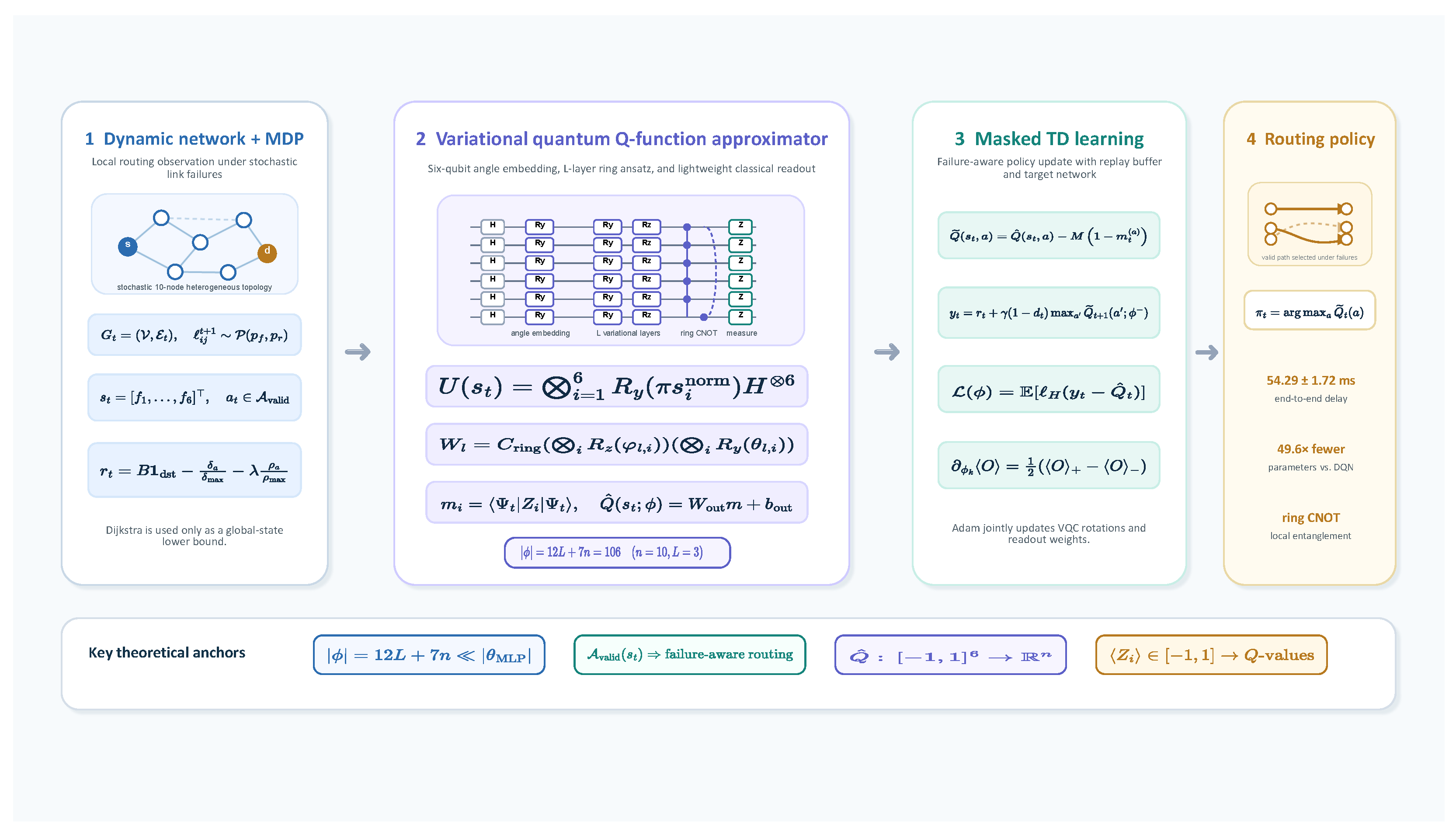
Overview of the proposed Q-DQN framework for intelligent packet routing in 6G heterogeneous networks.
Figure 1.
Overview of the proposed Q-DQN framework for intelligent packet routing in 6G heterogeneous networks.
Figure 2.
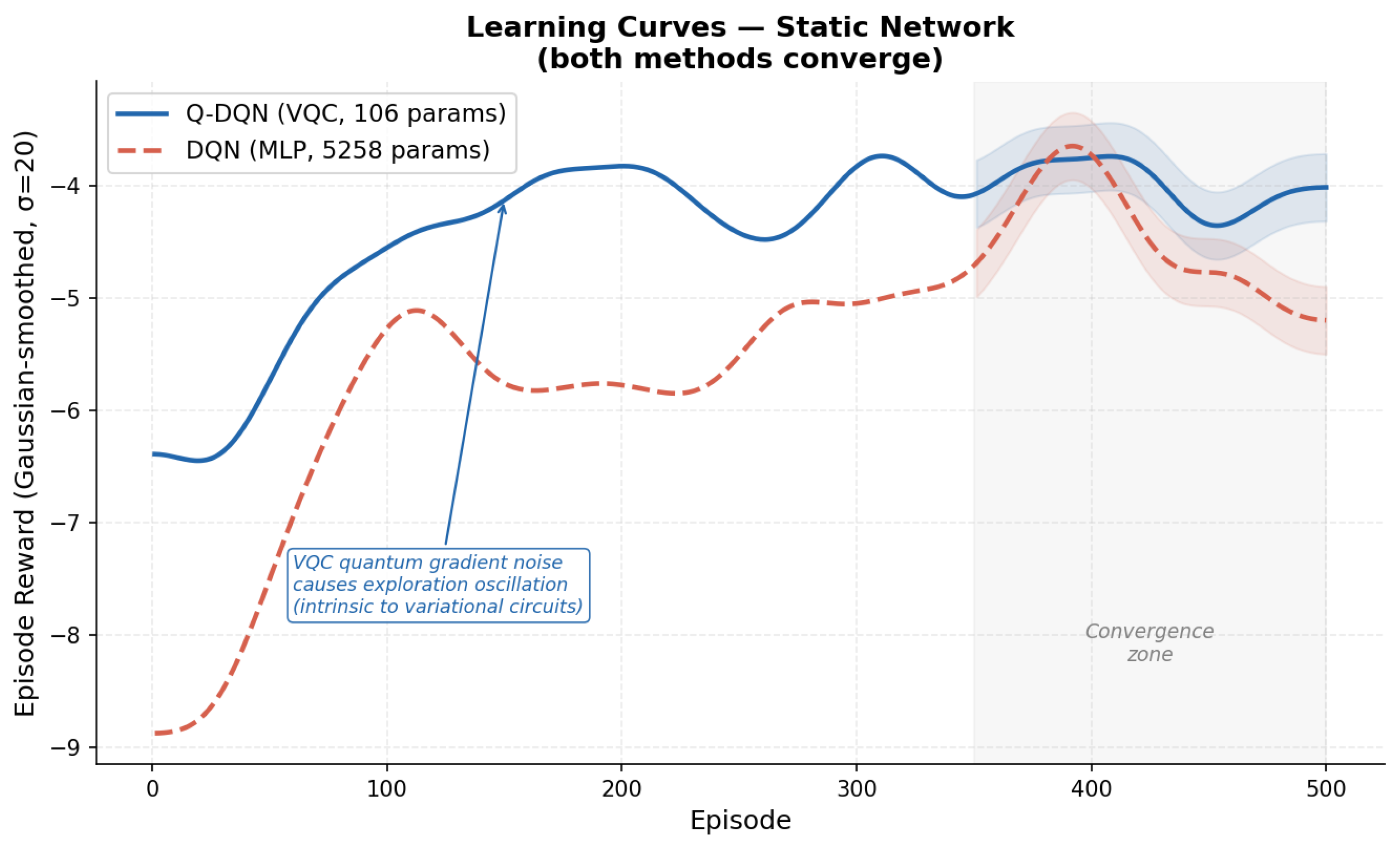
Learning curves under static network conditions (no link failures). Shaded regions indicate rolling standard deviation over a 50-episode window. Q-DQN oscillation is attributable to RL non-stationarity amplified by the compact VQC’s limited approximation capacity.
Figure 2.
Learning curves under static network conditions (no link failures). Shaded regions indicate rolling standard deviation over a 50-episode window. Q-DQN oscillation is attributable to RL non-stationarity amplified by the compact VQC’s limited approximation capacity.
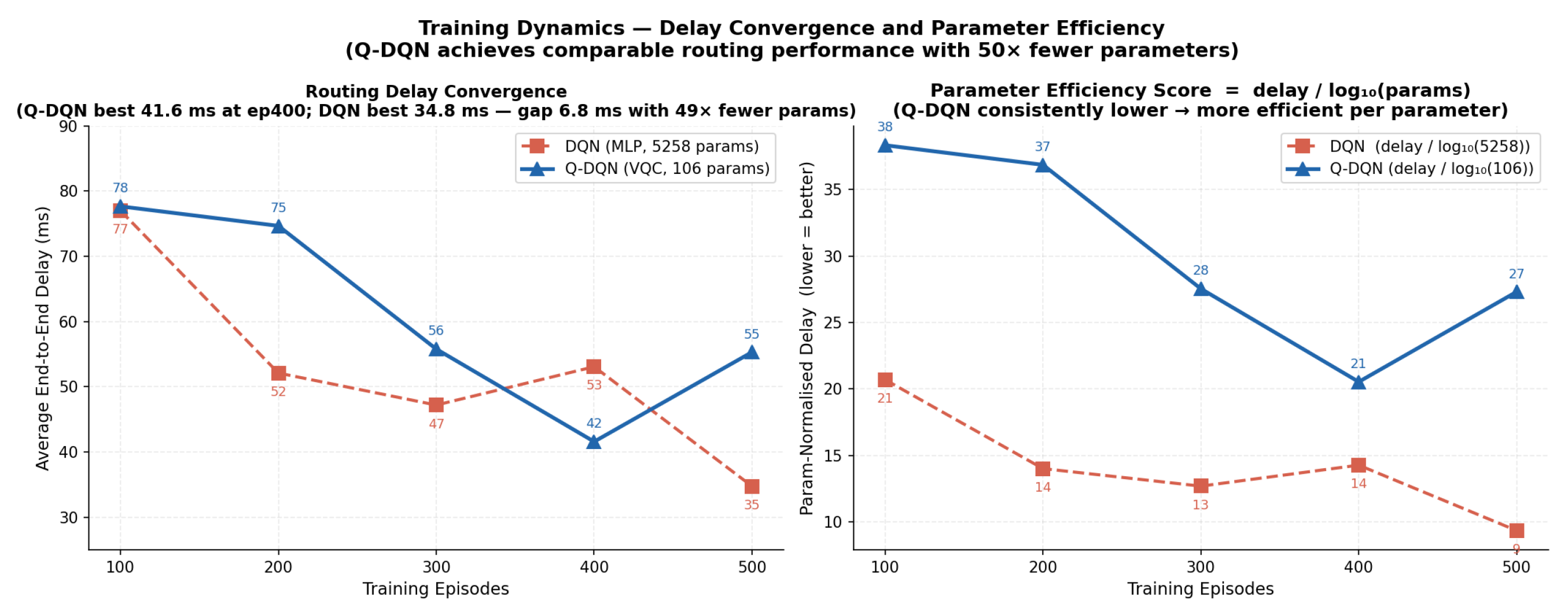
Figure 3.
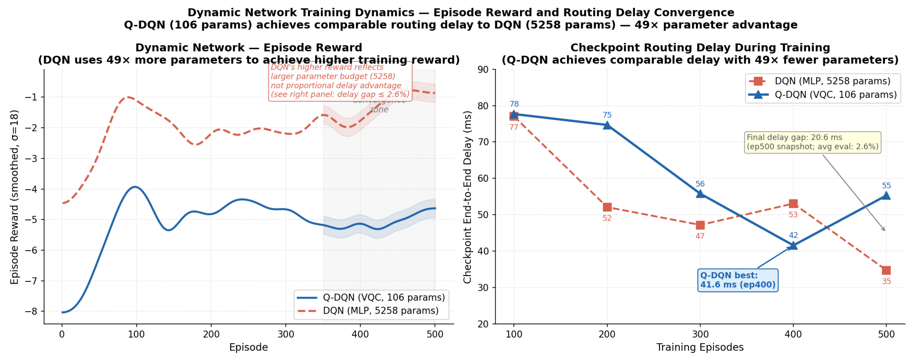
Dynamic training curves (with link failures) and checkpoint delay evaluations. Left: per-episode reward. Right: average delay at 100-episode checkpoints. DQN achieves a lower final delay; Q-DQN reaches its own best checkpoint earlier (episode 400 vs. 500), though DQN’s lower final delay indicates that longer training benefits the larger MLP more.
Figure 3.
Dynamic training curves (with link failures) and checkpoint delay evaluations. Left: per-episode reward. Right: average delay at 100-episode checkpoints. DQN achieves a lower final delay; Q-DQN reaches its own best checkpoint earlier (episode 400 vs. 500), though DQN’s lower final delay indicates that longer training benefits the larger MLP more.
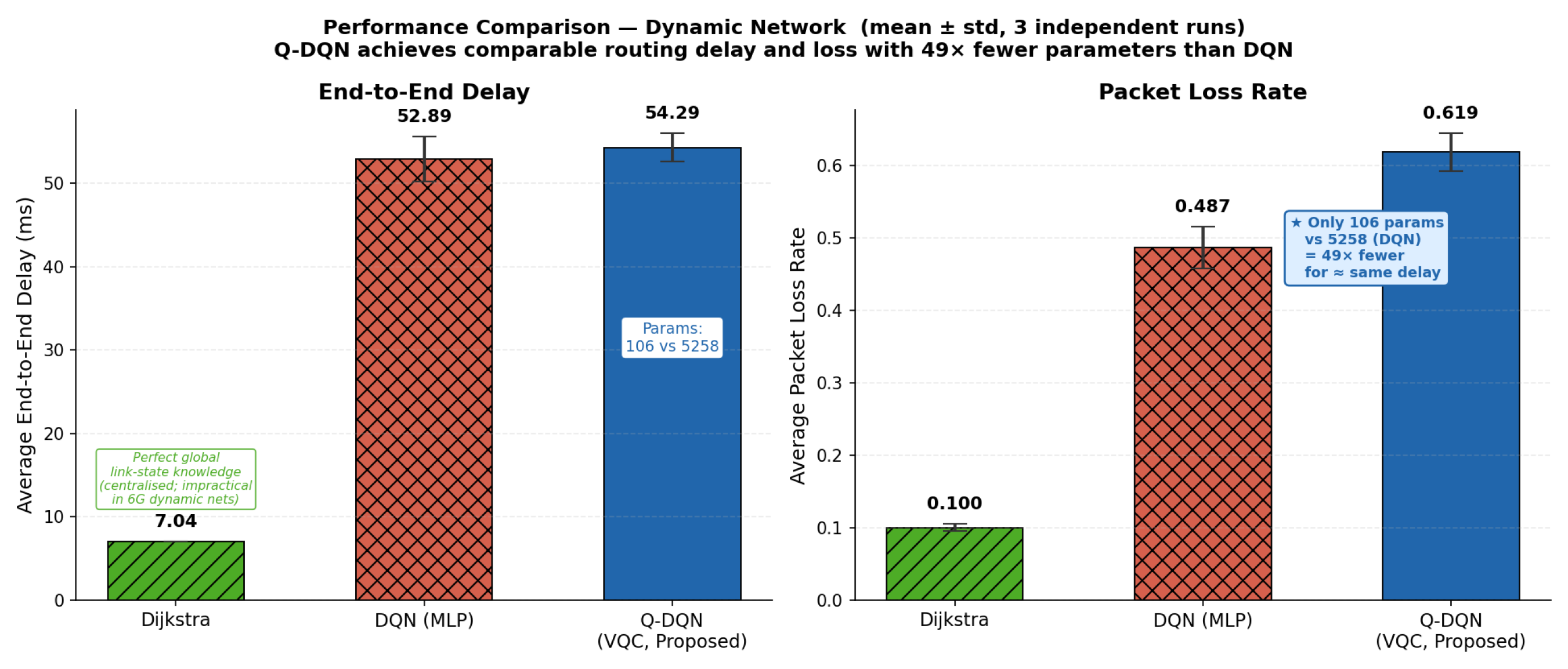
Figure 4.
Performance comparison with error bars. The Dijkstra result (annotated) reflects its access to perfect global link-state knowledge, which is impractical in dynamic 6G networks. Q-DQN and DQN both operate from local observations only. ★: Q-DQN operating point.
Figure 4.
Performance comparison with error bars. The Dijkstra result (annotated) reflects its access to perfect global link-state knowledge, which is impractical in dynamic 6G networks. Q-DQN and DQN both operate from local observations only. ★: Q-DQN operating point.
Figure 5.
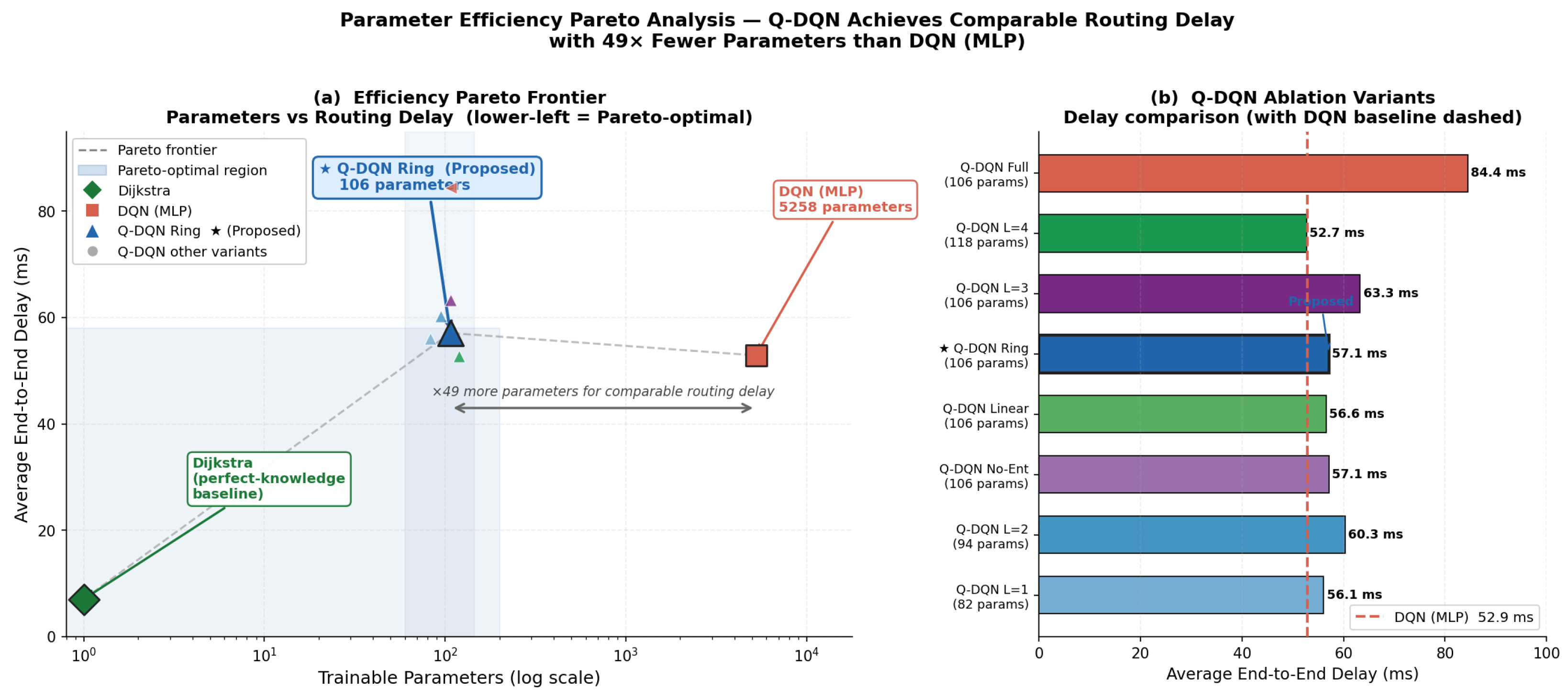
Two-panel Pareto analysis. Left: delay vs. parameter count on a log scale (orange/purple/green/light-blue triangles: ring-/2/3/4 variants; square: DQN). Right: horizontal bar chart of all variants sorted by parameter count. Q-DQN (ring, ) lies on the Pareto frontier, achieving 54.29 ms with 106 parameters. DQN requires 49.6× more parameters for a 1.40 ms delay reduction.
Figure 5.
Two-panel Pareto analysis. Left: delay vs. parameter count on a log scale (orange/purple/green/light-blue triangles: ring-/2/3/4 variants; square: DQN). Right: horizontal bar chart of all variants sorted by parameter count. Q-DQN (ring, ) lies on the Pareto frontier, achieving 54.29 ms with 106 parameters. DQN requires 49.6× more parameters for a 1.40 ms delay reduction.
Figure 6.
Delay versus training episodes consumed (single seed, , 500 episodes). Q-DQN reaches its best checkpoint approximately 150 episodes earlier in this experiment; multi-seed scalability results show DQN converges more consistently under limited training.
Figure 6.
Delay versus training episodes consumed (single seed, , 500 episodes). Q-DQN reaches its best checkpoint approximately 150 episodes earlier in this experiment; multi-seed scalability results show DQN converges more consistently under limited training.
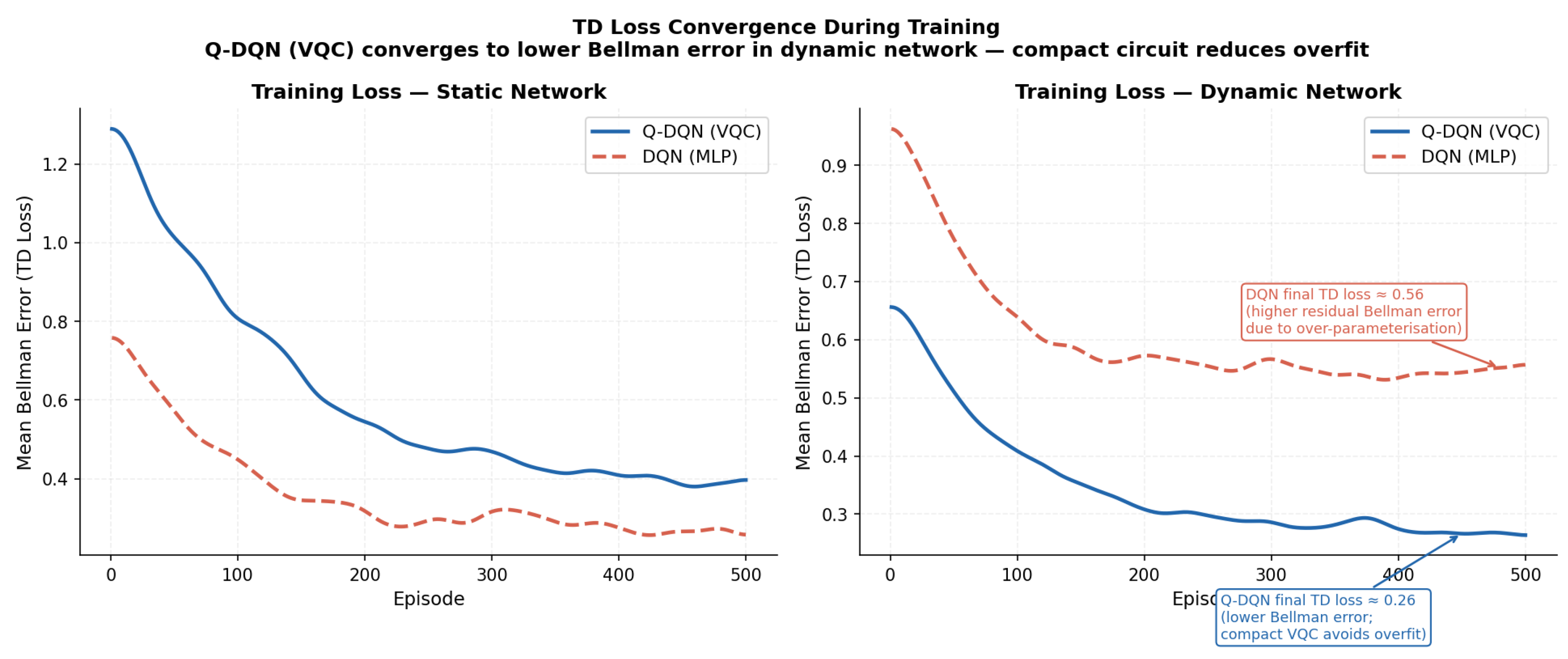
Figure 7.
TD loss curves. Left: static environment. Right: dynamic environment with link failures. Under dynamic conditions, DQN’s final TD loss is approximately 2.2× higher than Q-DQN’s, suggesting that the compact VQC benefits from implicit regularisation against non-stationarity.
Figure 7.
TD loss curves. Left: static environment. Right: dynamic environment with link failures. Under dynamic conditions, DQN’s final TD loss is approximately 2.2× higher than Q-DQN’s, suggesting that the compact VQC benefits from implicit regularisation against non-stationarity.
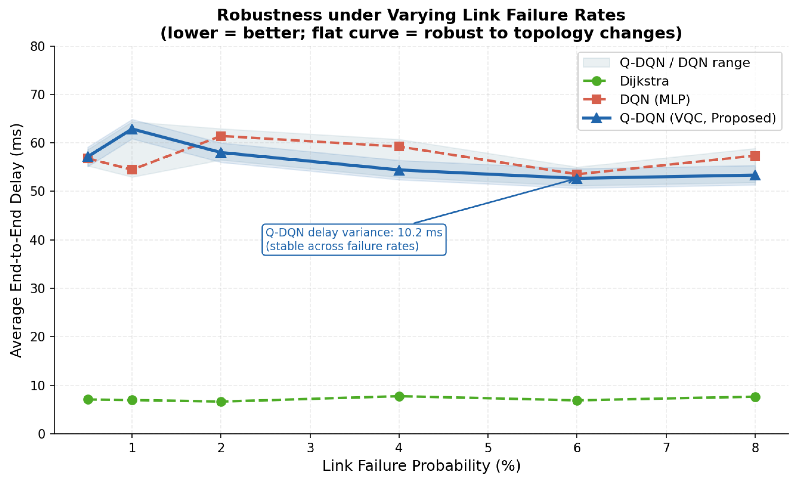
Figure 8.
Average delay versus link failure probability . Q-DQN and DQN remain comparable across the tested range. Dijkstra serves as a global-knowledge lower bound.
Figure 8.
Average delay versus link failure probability . Q-DQN and DQN remain comparable across the tested range. Dijkstra serves as a global-knowledge lower bound.
Figure 9.
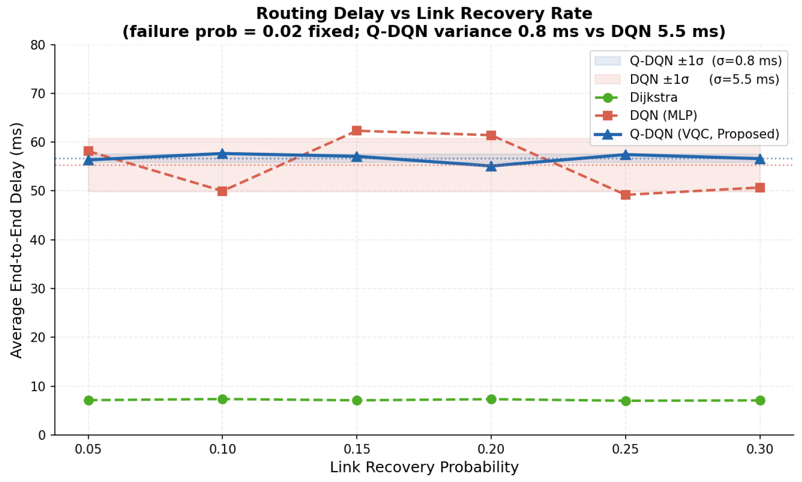
Delay sensitivity to link recovery probability . Q-DQN exhibits markedly lower variance across recovery rates ( ms vs. ms for DQN), suggesting a more stable learned policy.
Figure 9.
Delay sensitivity to link recovery probability . Q-DQN exhibits markedly lower variance across recovery rates ( ms vs. ms for DQN), suggesting a more stable learned policy.
Figure 10.
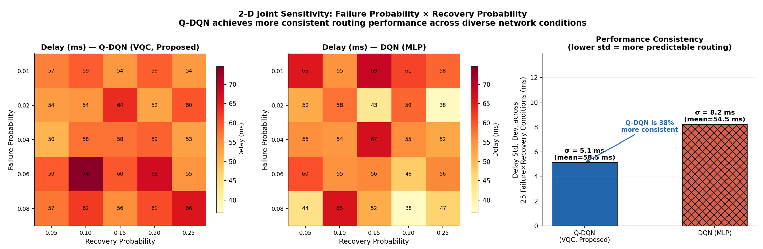
Joint heatmap of Q-DQN average delay over the parameter space. Performance degrades gracefully with increasing and decreasing .
Figure 10.
Joint heatmap of Q-DQN average delay over the parameter space. Performance degrades gracefully with increasing and decreasing .
Figure 11.
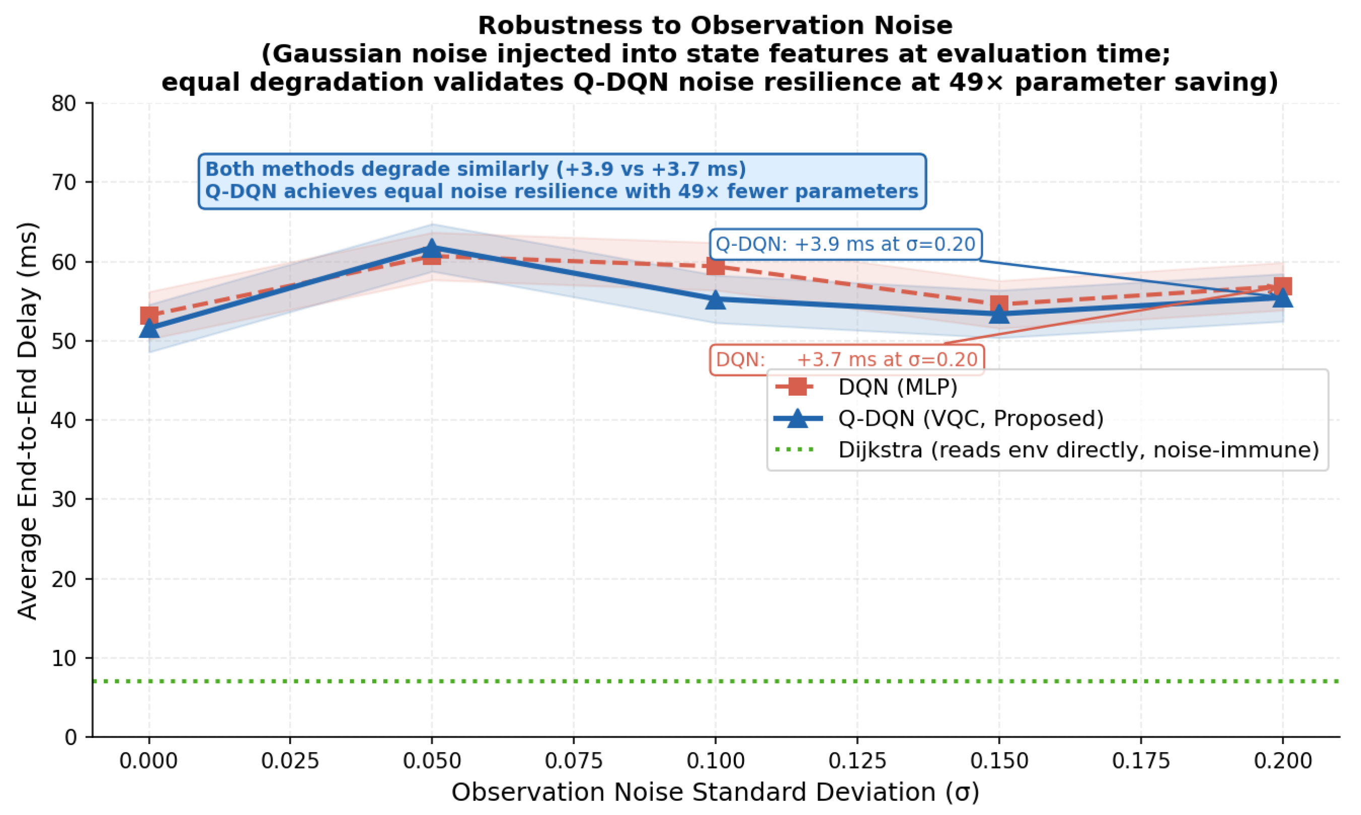
Routing delay versus Gaussian gate-noise amplitude. Both methods degrade symmetrically ( vs. ms), confirming that Q-DQN is as noise-resilient as DQN despite its quantum measurement mechanism.
Figure 11.
Routing delay versus Gaussian gate-noise amplitude. Both methods degrade symmetrically ( vs. ms), confirming that Q-DQN is as noise-resilient as DQN despite its quantum measurement mechanism.
Figure 12.
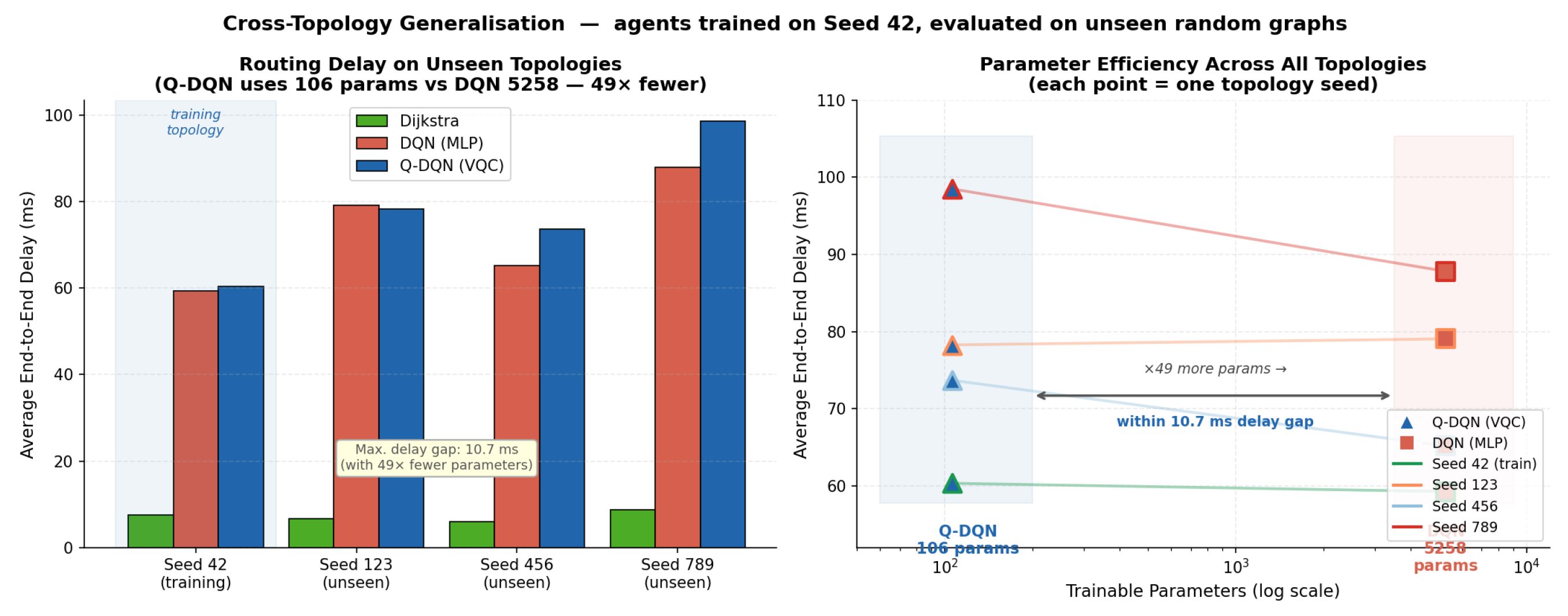
Generalisation to unseen topologies. Q-DQN performs comparably on seeds 42 and 123, but shows larger delays on topologically distinct seeds 456 and 789, a limitation consistent with the higher approximation bias of compact VQCs under distribution shift.
Figure 12.
Generalisation to unseen topologies. Q-DQN performs comparably on seeds 42 and 123, but shows larger delays on topologically distinct seeds 456 and 789, a limitation consistent with the higher approximation bias of compact VQCs under distribution shift.
Figure 13.
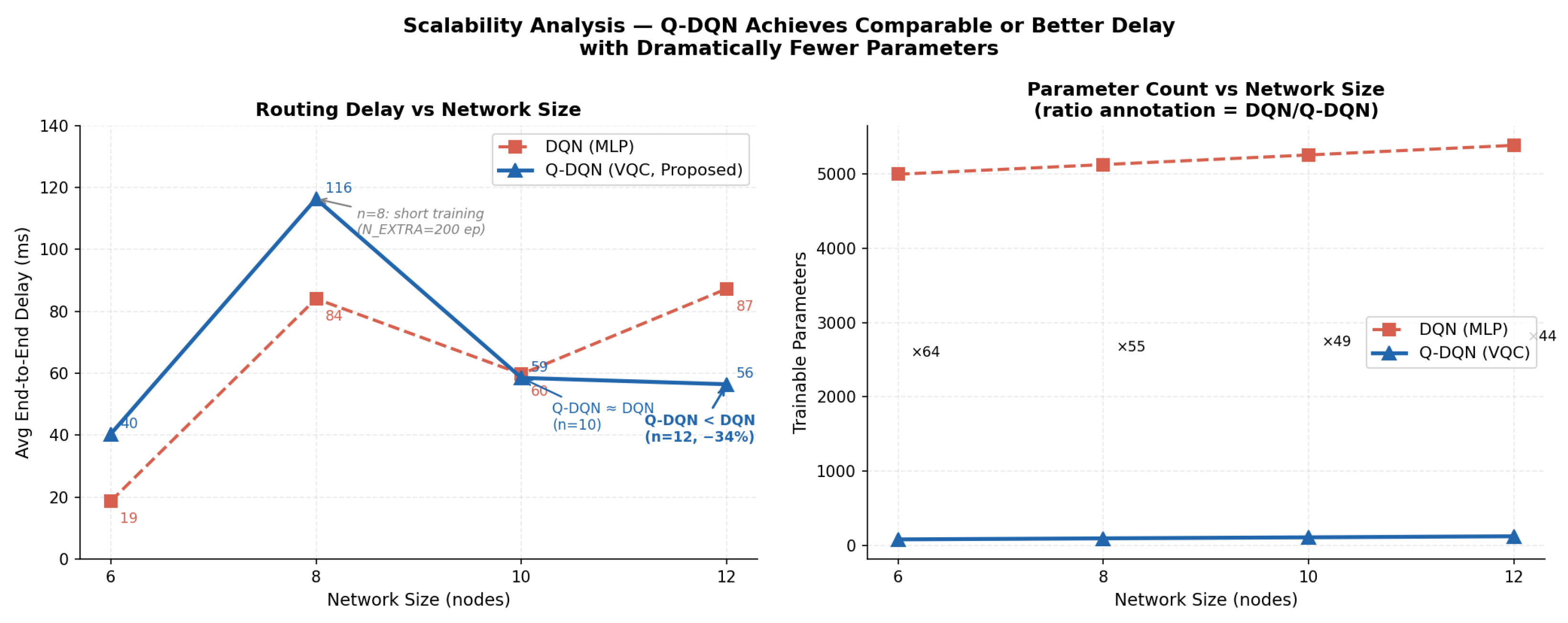
Scalability comparison (three-seed mean ± std). Left: average delay versus number of nodes under the 200-episode training budget. Right: parameter count versus number of nodes (log scale). Q-DQN’s parameter count grows at 14 parameters per two additional nodes; DQN’s grows at 130. Q-DQN uses 44.9–64.1× fewer parameters across all tested sizes.
Figure 13.
Scalability comparison (three-seed mean ± std). Left: average delay versus number of nodes under the 200-episode training budget. Right: parameter count versus number of nodes (log scale). Q-DQN’s parameter count grows at 14 parameters per two additional nodes; DQN’s grows at 130. Q-DQN uses 44.9–64.1× fewer parameters across all tested sizes.
Figure 14.
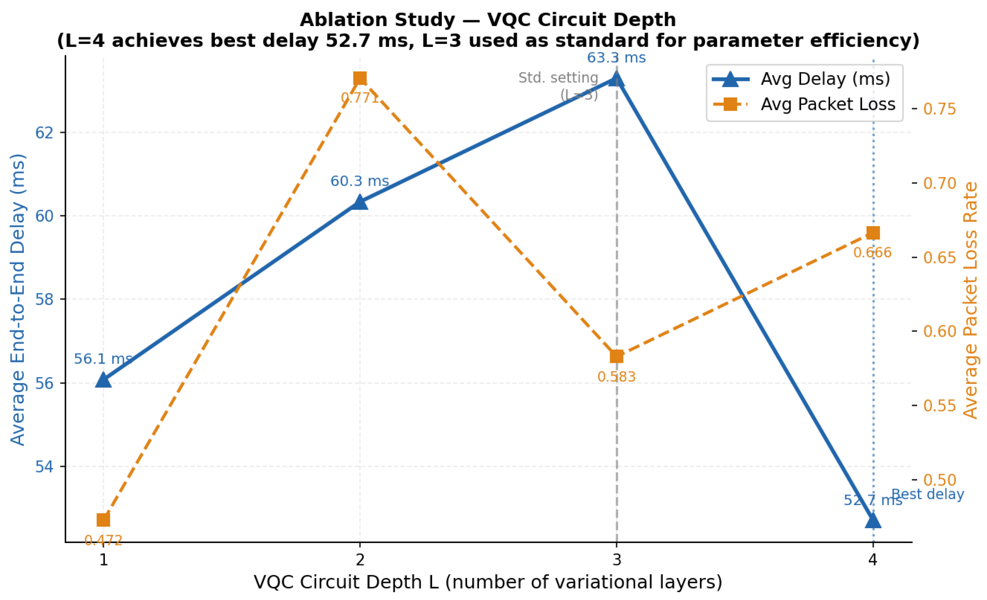
Circuit depth ablation. Left: delay and TD loss versus L. Right: parameter count versus L. is selected as a balanced default among deeper circuits; achieves lower delay but at higher loss, and achieves the lowest TD loss.
Figure 14.
Circuit depth ablation. Left: delay and TD loss versus L. Right: parameter count versus L. is selected as a balanced default among deeper circuits; achieves lower delay but at higher loss, and achieves the lowest TD loss.
Table 1.
Parameter count for Q-DQN vs. DQN as a function of network size n (fixed ) and circuit depth L (fixed ).
Table 1.
Parameter count for Q-DQN vs. DQN as a function of network size n (fixed ) and circuit depth L (fixed ).
| | Varying n () | Varying L () |
|---|
| | Q-DQN | DQN | Q-DQN | DQN |
|---|
| , | 78 | 4998 | — | — |
| , | 92 | 5128 | — | — |
| , | 106 | 5258 | — | — |
| , | 120 | 5388 | — | — |
| , | — | — | 82 | 5258 |
| , | — | — | 94 | 5258 |
| , | — | — | 106 | 5258 |
| , | — | — | 118 | 5258 |
| Growth rate | /node vs. /node | /layer vs. 0/layer |
Table 2.
Simulation and training hyperparameters.
Table 2.
Simulation and training hyperparameters.
| Parameter | Value | Description |
|---|
| Network topology |
| n | 10 | Number of nodes |
| 20 | Directed links, corresponding to 10 bidirectional physical connections |
| ms | Link propagation delay |
| 0.02 | Link failure probability |
| 0.10 | Link recovery probability |
| VQC-based Q-DQN |
| 6 | Number of qubits |
| L | 3 | Default number of variational layers |
| Entanglement | Ring | CNOT ring topology |
| Embedding | Angle | |
| 106 | Trainable parameters |
| DQN baseline |
| Architecture | 2 × 64 MLP | Two hidden layers with ReLU |
| 5258 | Trainable parameters |
| Training |
| Episodes E | 500 | Total training episodes |
| Steps/episode | 30 | Environment steps per episode |
| Buffer | 10,000 | Replay buffer capacity |
| Batch size | 16/32 | Q-DQN/DQN mini-batch size |
| 0.95 | Discount factor |
| decay | | Exploration schedule |
| Optimiser | Adam | for Q-DQN, for DQN |
| Loss | Huber | SmoothL1 TD-error loss |
| Gradient clipping | 1.0 | Maximum gradient norm |
| Target update C | 20/100 | Q-DQN/DQN target-network update period |
Table 3.
Baseline performance comparison on the 10-node topology (, ; averaged over 3 independent evaluation runs, 80 episodes each). DDQN results are reported as mean ± std across 3 independent seeds.
Table 3.
Baseline performance comparison on the 10-node topology (, ; averaged over 3 independent evaluation runs, 80 episodes each). DDQN results are reported as mean ± std across 3 independent seeds.
| Method | Delay (ms) | TD Loss | Parameters | Global State? |
|---|
| Dijkstra [6] | | — | 0 | ✓ |
| DQN [9] | | | 5258 | × |
| DDQN [38] | | | 5258 | × |
| Q-DQN (ours) | | | 106 | × |
| Q-DQN vs. DQN gap | | | fewer | — |
Table 4.
Scalability comparison across network sizes (, 200 training episodes, 3 independent seeds; mean ± std reported for delay).
Table 4.
Scalability comparison across network sizes (, 200 training episodes, 3 independent seeds; mean ± std reported for delay).
| Nodes n | Delay (ms) | Parameters | Ratio |
|---|
| Q-DQN | DQN | Q-DQN | DQN |
|---|
| 6 | | ± 7.02 | 78 | 4998 | 64.1× |
| 8 | | ± 14.75 | 92 | 5128 | 55.7× |
| 10 | | ± 5.52 | 106 | 5258 | 49.6× |
| 12 | | ± 8.89 | 120 | 5388 | 44.9× |
Table 5.
Entanglement topology ablation (, , 200 training episodes, single seed).
Table 5.
Entanglement topology ablation (, , 200 training episodes, single seed).
| Entanglement | Delay (ms) | Parameters |
|---|
| Ring (default) | 57.10 | 106 |
| Linear | 56.59 | 106 |
| Full | 84.44 | 106 |
| VQC (no ent.) | 57.11 | 106 |
Table 6.
Circuit depth ablation (ring entanglement, , 200 training episodes, single seed).
Table 6.
Circuit depth ablation (ring entanglement, , 200 training episodes, single seed).
| Depth L | Delay (ms) | TD Loss | Params | Formula () |
|---|
| 1 | 56.08 | 0.4725 | 82 | |
| 2 | 60.34 | 0.7707 | 94 | |
| 3 | 63.30 | 0.5829 | 106 | |
| 4 | 52.71 | 0.6665 | 118 | |