Article

CoDC: Unified Diffusion and Classification for Enhanced Class-Incremental Learning

School of Communication and Information Engineering, Shanghai University, Shanghai 200444, China
*
Author to whom correspondence should be addressed.
Appl. Sci. 2026, 16(12), 6035; https://doi.org/10.3390/app16126035
Submission received: 14 May 2026 / Revised: 2 June 2026 / Accepted: 11 June 2026 / Published: 15 June 2026
(This article belongs to the Section Computing and Artificial Intelligence)

Featured Application

Privacy-constrained visual recognition systems and systems with limited storage that must learn new classes continuously without retaining real samples from previous tasks.

Abstract

In class-incremental learning (CIL), a model must learn new classes while retaining previous knowledge without storing all historical data. Generative replay mitigates catastrophic forgetting by synthesizing old class samples, but conventional pipelines usually train separate generative and classification models and can be degraded by generated images of poor quality. This paper proposes the Co-Diffusion Classifier (CoDC), a unified framework based on diffusion that performs image generation and classification in a single network. CoDC attaches a classification branch to the UNet encoder and introduces an exponential noise filtering loss according to diffusion timesteps so that cleaner samples contribute more strongly to representation learning. A base task classification pre-training stage followed by collaborative training with selective parameter freezing reduces conflicts between noise prediction and semantic feature extraction. For rehearsal-free replay, generated samples are selected using confidence and feature consistency filters. Experiments on CIFAR-100, FaceScrub, and Flowers-102 show that CoDC maintains strong incremental accuracy without storing real old class exemplars. Additional comparisons that account for protocol differences with recent exemplar-free and pre-trained model methods clarify the setting in which CoDC is most directly comparable.

1. Introduction

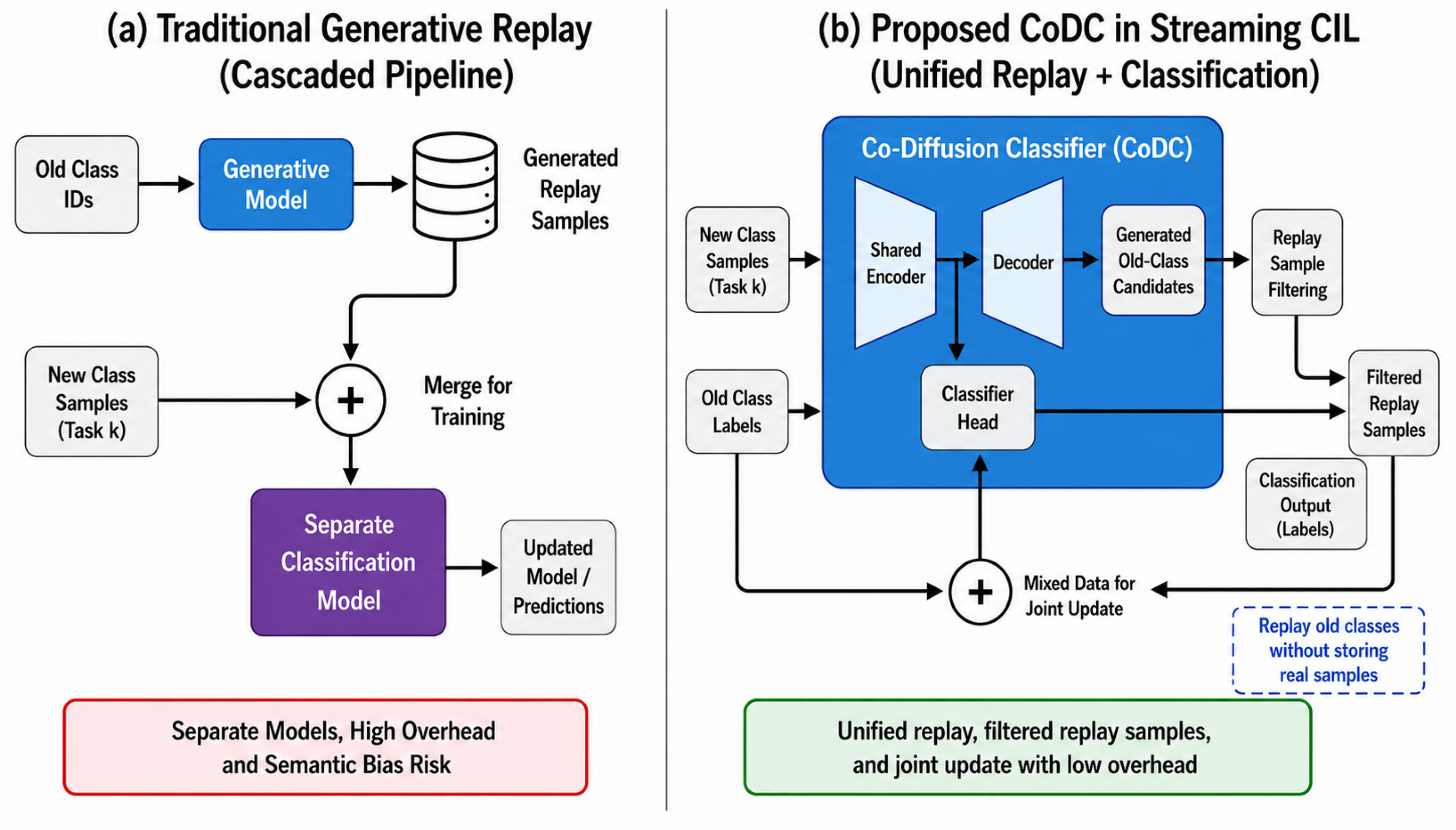
The typical training process for deep neural networks requires a collected dataset, such as large-scale images or text, over which the network iterates multiple times. However, in open-world scenarios, training data often arrives in a streaming format [1]. Due to storage limitations [2] or privacy concerns [3], this streaming data cannot be stored for the long term, requiring the model to be updated incrementally using only new class instances. This need has fostered the development of class-incremental learning (CIL) [4,5,6,7], which aims to build a classifier over all classes observed so far. A critical challenge in CIL is catastrophic forgetting [8], where optimizing a network with new classes erases knowledge of previously learned classes, leading to an irreversible decline in performance. Reducing catastrophic forgetting is therefore central to the design of CIL models. Traditional generative replay approaches employ a cascaded architecture where a generative model synthesizes samples from old classes, which are then used alongside new class samples to train a separate classifier. As illustrated in Figure 1a, this pipeline involves sequential processing through distinct models, resulting in high computational overhead and potential semantic bias from generated samples. In contrast, our proposed Co-Diffusion Classifier (CoDC) unifies these functionalities within a single diffusion model architecture, as shown in Figure 1b. By integrating generation and classification tasks, CoDC reduces computational cost while maintaining performance through joint optimization.
In a typical CIL setup, a model is evaluated on all previously seen classes after learning each new task. An ideal model should perform well on newly learned classes while retaining memory of old ones without forgetting. In practice, training data arrives sequentially at each step, forming a new training dataset (referred to as a “task”), and the model must be updated with these new classes. For instance, a model first learns “bird” and “dog” (Task 1), then “tiger” and “fish” (Task 2), followed by “monkey” and “sheep” (Task 3), and so on. After each task, the model is tested on all seen classes to assess its discriminative ability. A successful CIL model must balance learning features of new classes (plasticity) with preserving patterns of old classes (stability), a trade-off known as the “stability-plasticity dilemma” [8], where stability represents the ability to retain prior knowledge and plasticity represents the ability to adapt to new patterns. Continual and incremental learning were studied before the widespread adoption of deep learning. Early approaches mainly used traditional machine learning models and were often evaluated on a small number of incremental stages. Modern data streams require models that can be updated over longer sequences and larger class sets, making deep neural networks a suitable foundation for CIL. As a result, deep learning-based CIL has become an active research area in machine learning and computer vision.
Despite this progress, a clear research gap remains in strict CIL settings where real samples from previous classes cannot be retained. Memory-assisted methods can preserve old knowledge by storing exemplars, but this assumption is unsuitable for privacy sensitive applications or applications with limited storage. Generative replay avoids storing old images, yet existing replay pipelines are still insufficient in three aspects. First, they usually train a generator and a classifier as separate modules, which increases the model size, training cost, and maintenance complexity. Second, the classifier is trained on generated samples whose semantic quality is not guaranteed, so low fidelity or label ambiguous pseudo-samples can bias the decision boundary. Third, when diffusion-based generators are used, noisy intermediate samples contain different amounts of semantic information, but conventional replay does not explicitly control how much such noisy samples should affect representation learning. CoDC addresses this gap by coupling replay generation and classification in a shared diffusion network: the UNet encoder provides features for the classifier, the exponential timestep weighting reduces the influence of highly noisy samples on the classification loss, and confidence plus feature consistency filtering removes generated replay candidates that are semantically inconsistent with their target classes. Therefore, the central question is whether generation and classification can be coupled in one model while still controlling the noise and semantic mismatch introduced by generated replay.
This work addresses the following research questions:
  • RQ1: Can a single diffusion model support both old class image generation and discriminative classification for class-incremental learning?
  • RQ2: How can the classifier use noisy diffusion samples without learning noise-contaminated features?
  • RQ3: Can generated samples replace real exemplar storage under a strict zero memory protocol?
The main contributions are summarized as follows:
  • We propose CoDC, a unified diffusion-classification architecture that attaches a classification branch to the UNet encoder and performs generation and classification within one network.
  • We design an exponential noise filtering mechanism that weights the classification loss according to the diffusion timestep, reducing the impact of highly noisy samples.
  • We introduce a base task classification pre-training stage followed by collaborative training with parameter freezing to reduce conflicts between noise prediction and semantic feature extraction.
  • We develop a rehearsal-free generative replay procedure that selects generated old class samples using confidence and feature consistency before combining them with current new class data.
  • We report comparisons under both strict zero memory and mixed memory protocols to clarify when CoDC is directly comparable with existing baselines.
The implementation of CoDC is publicly available at https://github.com/896393962/CoDC-CIL, accessed on 10 June 2026.

2. Related Work

2.1. Class-Incremental Learning

Recent work has advanced this field in machine learning and computer vision. Recent journal surveys have clarified the distinctions among task-incremental, domain-incremental, and class-incremental learning, and have emphasized that CIL is especially challenging because the model must discriminate among all classes seen so far without task identity at inference time [5,6,7,9]. To mitigate catastrophic forgetting in CIL, existing methods can be broadly categorized into parameter regularization, knowledge distillation, data replay, and architectural approaches. Parameter regularization methods constrain important parameters during incremental updates. For instance, EWC [10] was a pioneering work that constrained important parameters using the Fisher information matrix to estimate their importance, thereby reducing forgetting. During the model training phase, the importance of each parameter is calculated by accumulating the sensitivity of the loss function to changes in each parameter. Knowledge distillation methods maintain consistency between the outputs of the old and new models for a given input while learning a new task. The old model is the one that has finished learning the previous task, and the new model inherits the parameters of the old model and can be updated on the new task. This requires introducing an additional distillation loss during network training to reduce the forgetting of old class knowledge. For example, LwF (Learning without Forgetting) [11] introduced a distillation loss that minimizes the KL divergence between the probability distributions of the old and new models, preserving knowledge of old classes. Data replay methods can be divided into two categories: storing a small subset of real samples from past classes (rehearsal) and generating pseudo-samples. Replay remains one of the most effective families of continual learning strategies, but recent journal studies also note that replay becomes problematic when privacy, storage, or long streams prevent retaining historical examples [12,13]. The original teacher–student formulation of knowledge distillation is also relevant to this family of methods [14]. Regardless of whether the samples are real or pseudo, these old class data are used together with new class data to update the current model. Combining old and new class data in this way reduces catastrophic forgetting during the incremental learning process. For example, iCaRL [15] is a prominent rehearsal method that stores a fixed number of exemplars for each old class, selected using a nearest-mean-of-exemplars (NME) strategy. To address privacy concerns, generative replay methods use models such as autoencoders or GANs [13,16,17], including the Closed-loop Memory Replay GAN (CloGAN), to synthesize pseudo-samples of old classes for joint training. More recently, diffusion models [18,19] have also been used. Our work falls into this category but introduces a unified architecture that eliminates the need for a separate generative model and classifier. Architectural methods dynamically adjust the model’s capacity to accommodate new classes. For example, DER (Dynamically Expandable Representation) [20] dynamically expands the network by adding a new feature extractor for each incremental task while freezing the old ones. The features from all extractors are concatenated before being fed to the classifier, preserving old knowledge while providing capacity for new learning. These categories are not mutually exclusive and have no strict boundaries; they provide a practical way to analyze the development of class-incremental learning from different perspectives. Recent exemplar-free CIL methods further focus on compensating feature or semantic drift without retaining old images. Representative examples include FeTrIL [21], SEED [22], and DPCR [23]. These methods are highly relevant to our setting because they avoid exemplar buffers, but their published protocols still differ in task split, backbone, and whether the method is rerun under a small start or big start setting. We therefore report the protocol source explicitly in the experimental comparison instead of mixing all numbers into a single ranking.
In parallel, pre-trained model-based CIL has become an active direction. Methods such as RanPAC [24], EASE [25], TUNA [26], and SplitLoRA [27] use large pre-trained ViT backbones and parameter-efficient adaptation, while DiffClass [18] relies on a pre-trained diffusion model. These approaches provide recent reference results for settings with external pre-training. However, because they exploit large-scale pre-training and different computational assumptions, we separate them from methods with standard backbones and use them only as reference comparisons.

2.2. Diffusion Models

Diffusion models [28,29,30] are a class of generative models that have recently gained prominence. They operate by progressively adding Gaussian noise to data in a “forward process” and then learning to reverse this process to generate data from noise in a “reverse process.” The core of this process lies in learning the denoising process to generate data. The diffusion process is typically divided into multiple timesteps t { 1 , , T } , with each timestep corresponding to a different “noisy” state of the data. The objective is to learn how to recover the original data from a state of complete noise. In image diffusion models, a UNet architecture [31] is commonly used as the denoising backbone. The number of timesteps, T, controls the noising and denoising process; a smaller T results in a milder noising process where the data retains more of its original features, but the generated samples may lack detail or appear blurry. A larger T allows the data to approach complete noise, making the denoising process more complex and improving the quality of generated images, but at the cost of increased computation. Subsequent works like DDIM [32] have focused on faster sampling, while Latent Diffusion Models (LDMs) [33] perform the diffusion process in a lower-dimensional latent space to improve efficiency. This approach achieves a good balance between the speed and quality of image generation. Meanwhile, the potential of diffusion models has also been extended to audio processing [34] and text-to-3D generation [35]. Our work leverages the UNet backbone of diffusion models and repurposes its encoder for classification in a multi-task learning framework.

2.3. POD Loss Function

The Predefined Optimal-distribution Loss (POD Loss) [36] aims to maximize inter-class distances while minimizing intra-class distances in the latent feature space. Instead of using a SoftMax layer to constrain posterior probabilities, it directly uses a cosine loss on the features, which has been shown to achieve superior classification performance. The loss is formulated as follows:
L p o d = 1 N i = 1 N 1 cos N ( θ y i ) 2 + λ j i , n j n i R i j 2
cos N ( θ y i ) = cos ( θ y i ) 1 + δ e M / | x i |
R = 1 B 1 X X p e d c c X X p e d c c T
where N is the number of training samples, i indexes a sample, x i is the feature vector of the i-th sample, | x i | is its feature magnitude, y i is its class label, and θ y i denotes the angle between x i and the predefined target vector of class y i . The term cos N ( θ y i ) is the magnitude-normalized cosine score used by POD Loss. λ controls the strength of the decorrelation term, R i j is the ( i , j ) entry of the correlation matrix R, and n i and n j denote the class indices associated with the corresponding feature outputs when identifying inter-class pairs. The parameter δ is a scaling factor used to amplify the effect of samples with smaller magnitudes, M is the average feature magnitude in the current training stage, and e denotes the current training epoch. B is the batch size, X is the matrix of network feature outputs in a mini-batch, and X p e d c c is the matrix of predefined target feature vectors. POD Loss focuses on the classification accuracy of hard samples via δ and reduces linear redundancy in the network output through the correlation matrix R.

3. Materials and Methods

To address the challenges of high computational cost and semantic deviation in generative replay, we propose the Co-Diffusion Classifier (CoDC), a unified network for image generation and classification.

3.1. Collaborative Generation and Classification Architecture

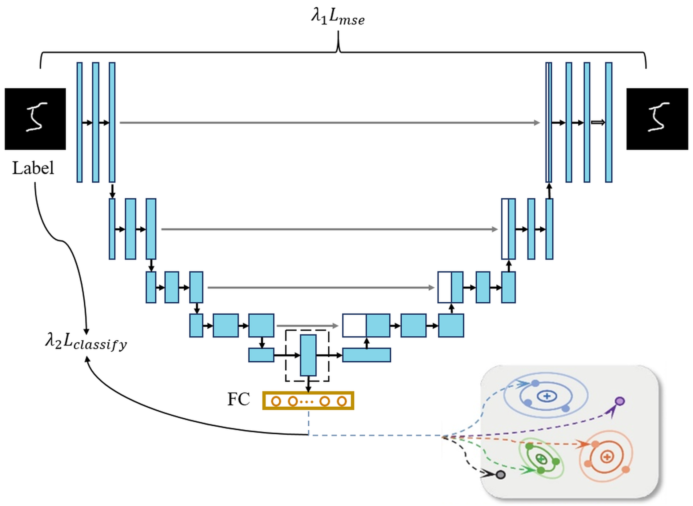
In diffusion models, the UNet is used as the core component of the generative network. This paper proposes a method that aims to simultaneously perform feature extraction tasks by leveraging the UNet encoder (the left half of the UNet) during the training process of the diffusion model. Specifically, while training the diffusion model to predict noise, features are extracted from an intermediate layer of the encoder for an image classification task, thereby forming a dual task learning framework, as shown in Figure 2. However, a standard UNet architecture, when compared to a dedicated classification network like ResNet50, often lacks the necessary depth for abstract feature representation. For instance, a ResNet50 adapted for 64 × 64 images contains a deep stack of residual blocks, whereas a typical UNet encoder has fewer convolutional blocks, limiting its feature extraction capacity. To address this, we enhance the UNet encoder by increasing its depth (i.e., the number of residual blocks per stage), enabling it to learn more discriminative representations for classification while retaining its generative function. To achieve dual task learning, a classification branch is introduced into the network, and a composite loss function is designed. Therefore, the total loss function of the network consists of two parts (Equation (4)): the first part is the mean squared error (MSE) loss for the noise prediction task of generation, and the second part is the classification loss for the classification task. We employ POD Loss for L c l a s s i f y due to its effectiveness in creating a geometrically optimal feature space by enforcing orthogonality between class centroids. These two parts work together to constrain the network parameters, theoretically enabling the network to have both generation and classification capabilities.
L t o t a l = λ 1 L m s e + λ 2 L c l a s s i f y
However, in practice, the noisy images can contaminate the feature extraction process, thereby severely degrading classification performance.

3.2. Noise Filtering Mechanism

To address the issue of noise pollution, it is first necessary to understand how diffusion models progressively inject noise into an image. In a diffusion model, as the timestep t increases (from t = 0 to t = 999 ), more noise is added to the image. This is achieved through the mathematical design of the noise schedule parameter β t . We adopt a linear schedule for β t :
β t = β m i n + t T ( β m a x β m i n )
where β m i n and β m a x are the initial and final noise variances of the linear schedule, respectively. For compact notation in the following derivation, we define Δ β = β m a x β m i n as the total increase in the noise variance over the diffusion process. The forward noising process of the diffusion model can be defined by the following formulas:
x t = α ¯ t x 0 + 1 α ¯ t ϵ , ϵ N ( 0 , I )
where α ¯ t = i = 1 t α i and α t = 1 β t . Here, α ¯ t represents the cumulative signal decay coefficient from the initial state x 0 to step t. In this subsection, t denotes the diffusion timestep and T is the total number of diffusion steps. For clarity, t is used only for diffusion timesteps, while k denotes the incremental task index in the CIL procedure. As t increases from 0 to T, α ¯ t monotonically decreases to 0, meaning the image x t becomes progressively dominated by noise; this signal decay trend motivates the weighting by the timestep introduced below.
Our key insight is that samples with low noise (small t) contain more semantic information and are more valuable for training the classifier. Therefore, we propose a weighted loss strategy where the contribution of L c l a s s i f y for each sample is weighted based on its timestep t. To derive a precise weighting function, we analyzed the relationship between the cumulative signal rate α ¯ t and the timestep t. The formula for α ¯ t can be expressed as:
ln α ¯ t = i = 0 t ln ( 1 β i )
Given that β i 1 , we can use a Taylor expansion for ln ( 1 β i ) and truncate it to the second order:
ln ( 1 β i ) β i β i 2 2
This leads to the approximation:
ln α ¯ t i = 0 t β i 1 2 i = 0 t β i 2
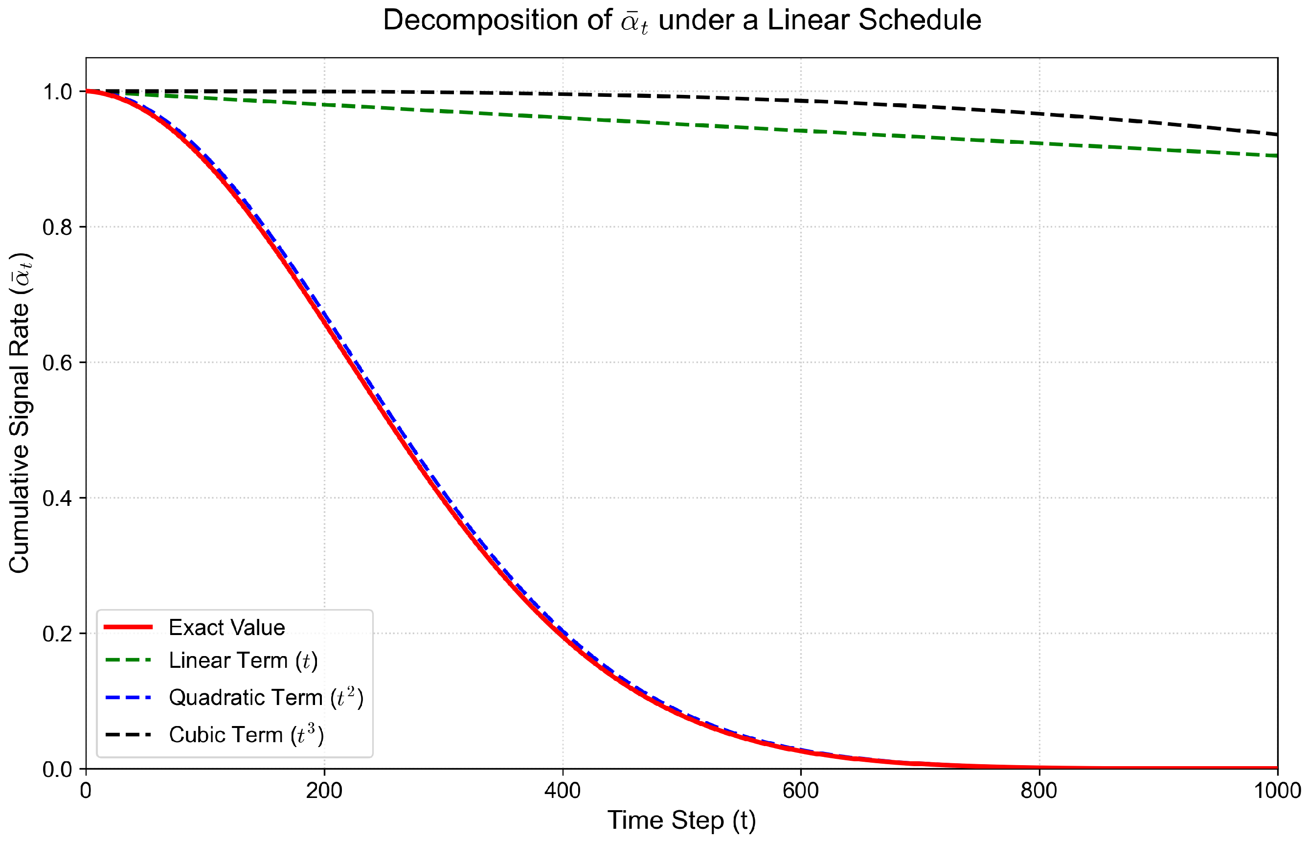
From this, we can see that α ¯ t has an exponential relationship with the powers of t. As shown in Figure 3, the evolution of α ¯ t is most strongly correlated with the t 2 term. This justifies our design of an exponential noise filtering algorithm where the weight is a function of t 2 , as defined in Equation (11). This ensures that the weights assigned to the classification loss accurately reflect the ratio between signal and noise at each timestep.
α ¯ t exp ( t ( β m i n + β m i n 2 2 ) t 2 T ( Δ β 2 + β m i n 2 Δ β ) t 3 6 T 2 Δ β 2 )
Equation (10) is used to derive the weighting function for the classification loss. As depicted in Figure 3, an analysis of the different power terms of t in this expression shows a strong correlation between α ¯ t and the t 2 term. Therefore, we design an exponential noise filtering algorithm. After substituting the set values, the weight for a sample at timestep t is defined as:
weight ( t ) = exp t 2 T ( Δ β 2 + β m i n 2 Δ β ) e t 2 / 10 5
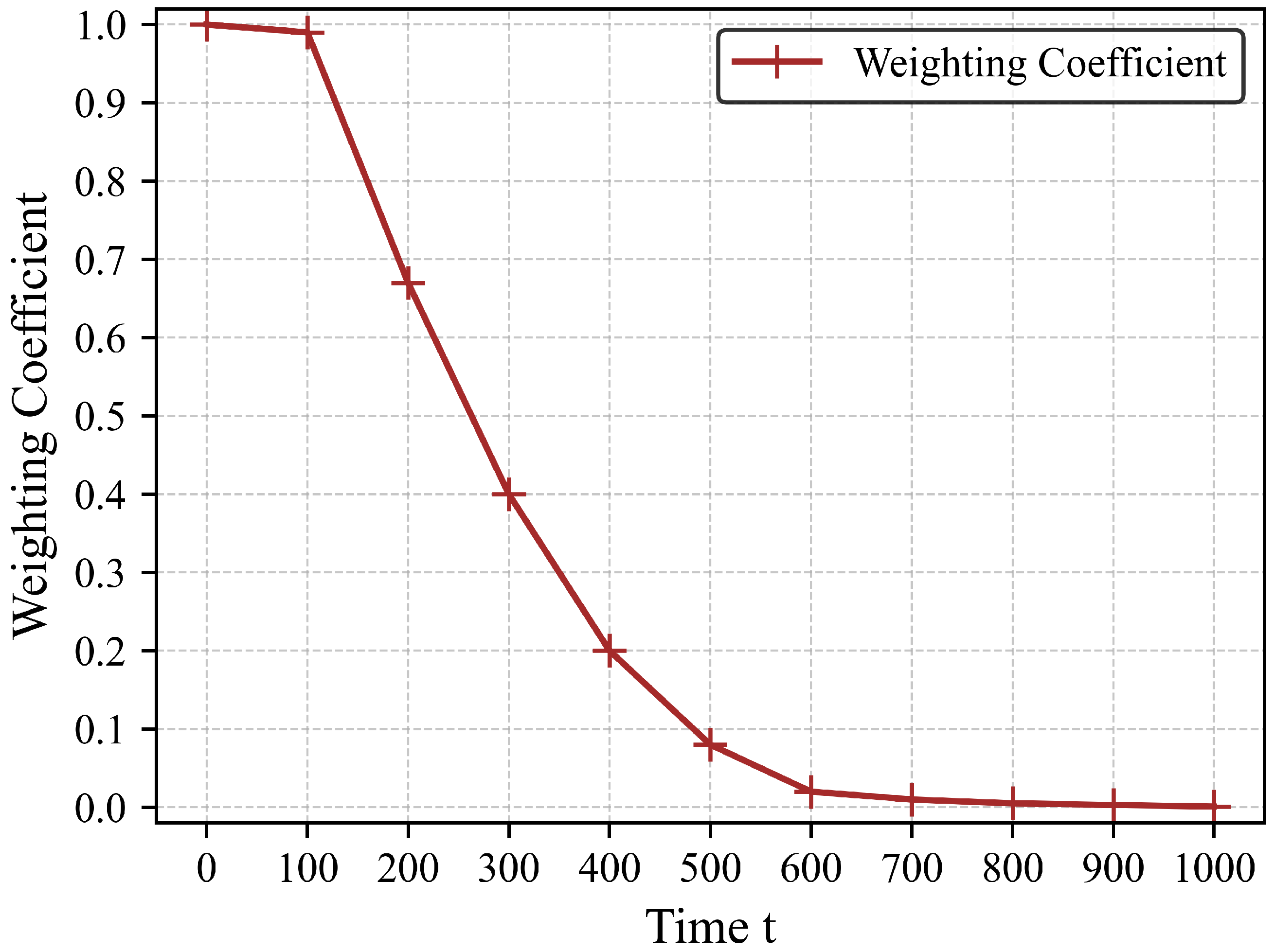
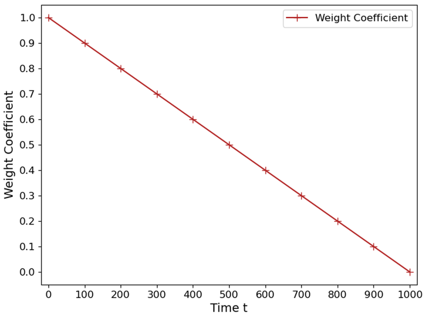
As shown in Figure 4, this function assigns high weights to samples with low noise (small t) and exponentially decaying weights as t increases, reducing the influence of highly noisy samples on the classification task. This exponential rule is the default noise filtering strategy used by CoDC.

3.3. Two-Step Training with Parameter Freezing

The dual objectives of noise prediction (for generation) and feature extraction (for classification) are inherently contradictory. The former aims to model a noisy distribution, while the latter seeks to filter out noise to capture clean semantics. This conflict can lead to suboptimal performance for both tasks. To address this, we use a two stage initialization and collaborative training scheme in which Stage 1 is applied only to the base task. The rationale for freezing deeper encoder blocks is grounded in the hierarchical nature of feature extraction in deep neural networks. Deeper layers are known to capture abstract semantic information that is critical for discriminating between classes (e.g., the overall shape of an object). In contrast, shallower layers capture more generic visual patterns such as edges and textures. In our collaborative architecture, the generation task, which involves modeling noise, primarily conflicts with the extraction of abstract semantics. By freezing the deep encoder layers after the base task classification pre-training, we protect these semantic representations from being corrupted by the noise prediction objective. This allows the shallower layers to remain plastic and adapt to the dual task loss, balancing the need for stable semantic features for classification with the flexible feature adjustments required for high quality image generation. This targeted freezing strategy is key to mitigating task conflict and preventing the degradation of the model’s classification capabilities. Stage 1: Base Task Classification Pre-training. Stage 1 is performed only once on the base task. We first train the CoDC network using only the classification loss ( L c l a s s i f y ) and the real samples from the base classes. This allows the UNet encoder to develop stable and discriminative semantic features without interference from the noise prediction task before incremental learning begins. Stage 2: Collaborative Training with Parameter Freezing. After this base task pre-training stage, we freeze the parameters of the deeper blocks of the UNet encoder. These deep layers capture abstract, task-specific semantic information required for classification. By freezing them, we preserve the stability of the learned feature space. The shallower layers, which extract more general visual features, remain trainable, along with the decoder and classification head. The model is then trained on the full collaborative loss ( L t o t a l ). This collaborative stage is used for the base task after Stage 1 and for all subsequent incremental tasks; Stage 1 is not repeated for later tasks. This approach allows the network to adapt its early feature extraction and generative capabilities while protecting the core semantic representations from being corrupted by the noise prediction objective.

3.4. Rehearsal-Free Generative Replay

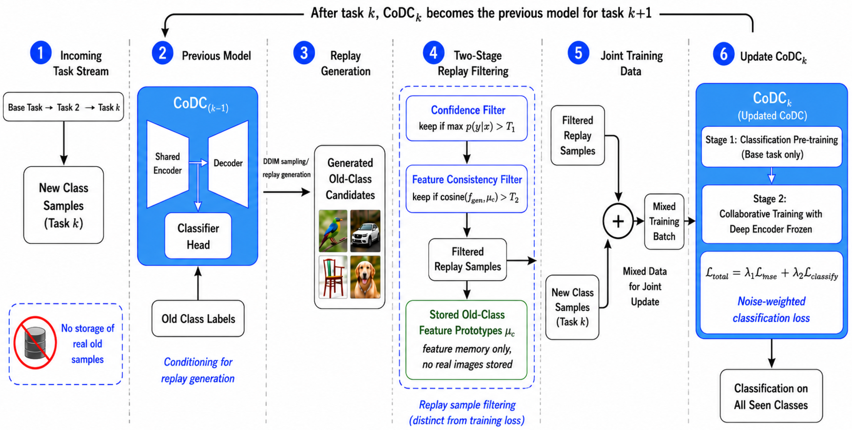
With the collaborative network, we can implement a generative replay strategy for CIL that requires no storage of real data. The complete streaming procedure is illustrated in Figure 5 and is summarized as follows. At incremental step k, the training data contain only the real samples of the newly arriving classes. Here, k indexes the incremental learning task and is distinct from the diffusion timestep t used in the noise-filtering derivation. Before updating the model on these new classes, the CoDC model learned after step k 1 generates pseudo-samples for previously seen classes. These generated old class samples are screened by the confidence and feature consistency criteria described below. The retained generated samples are then merged with the real samples from the current step, and the combined set is used to update CoDC with the collaborative objective. In these later incremental steps, the base task classification pre-training stage is not repeated. After training at step k, the real samples from the current step are discarded; only the model parameters and lightweight feature statistics used for filtering are kept. Thus, the replay set used during incremental learning contains generated images rather than stored real old class exemplars.
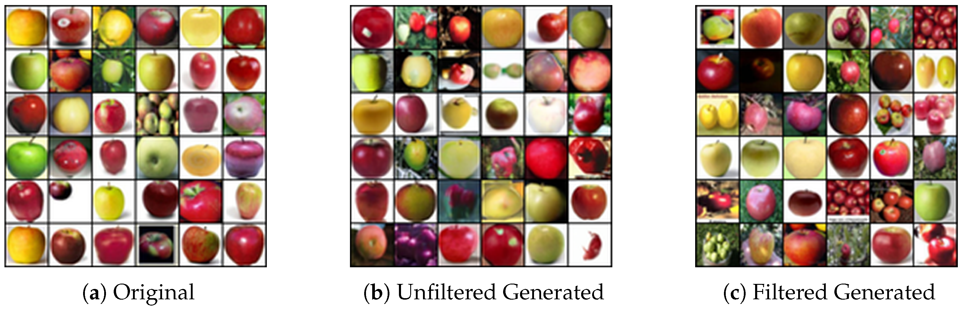
Although diffusion models can synthesize visually realistic images, the discrepancy between the distribution of generated images and the original training distribution remains an underexplored issue. For instance, a diffusion model trained on a certain dataset to generate 100 images of class A might occasionally produce a few images that resemble other classes (negative samples). This discrepancy can stem from training data bias or sampling stochasticity. Because generated images are used as replay data in CIL, it is important to select generated samples that reduce the distribution gap between generated and real data. Therefore, to address this issue, we propose a two-step filtering strategy to select only generated samples of high quality, as illustrated in Figure 6. (1) Confidence-Based Filtering: The core idea is to filter out generated images that do not match their class labels based on classification confidence. That is, during the image generation process, specifically at the last denoising step, we use the output probability from the UNet’s classification head to screen for samples with high confidence and filter out ambiguous samples with low confidence. This method naturally leverages the advantage of the collaborative network. The confidence is calculated as follows:
F 1 = max p ( y = y i | x i ) > T 1
We set a threshold T 1 (e.g., 0.80). If the confidence is greater than T 1 , the image is retained as replay data. Otherwise, it is discarded. (2) Feature Consistency Filtering: Using only filtering based on confidence might still allow some “deceptive” samples to pass through. To mitigate this, we introduce filtering based on feature space consistency. First, when a class is learned, we compute and retain its mean feature vector μ c from encoder features and normalize it using L2 normalization. This stores a compact feature statistic rather than retaining the original images. Then, during image generation, at the final denoising step, we extract the feature vector f x g e n of the generated image, also perform L2 normalization, and finally calculate the cosine similarity with the class mean.
cos ( θ ) = f x g e n · μ c f x g e n μ c > T 2
A sample is accepted only if its similarity is above threshold T 2 (e.g., 0.75). This ensures that the generated exemplars not only have high confidence but also cluster tightly around the class centroid in the feature space. In our experiments, we first apply the confidence threshold, followed by the feature cosine similarity, to select the most suitable generated images for data replay.

3.5. Experimental Protocol

Datasets: We evaluate our method on three benchmark datasets: CIFAR-100 [37], a 100-class dataset of 32 × 32 images; FaceScrub [38], a fine-grained face dataset with 100 identities and 64 × 64 images; and Flowers-102 [39], a fine-grained flower dataset where we use the first 100 classes with 64 × 64 images. For Flowers-102, each class has 30 training samples and 7 test samples. Incremental Settings: We use two task protocols. In Scenario 1, the model starts from 20 base classes and then learns four increments of 20 classes. In Scenario 2, the model starts from 50 base classes and then learns five increments of 10 classes. Unless otherwise stated, the class order is fixed across methods, and the random seed is set to 1993 in the reproduced baseline runs. Evaluation Metrics: In the context of CIL, researchers commonly use incremental accuracy and forgetting rate as performance evaluation tools.
  • Incremental Accuracy (A): The average classification accuracy across all incremental tasks at the end of the entire learning process. Given K tasks, let A k be the accuracy on all seen classes after task k. The final average accuracy is:
    A = 1 K k = 1 K A k
  • Average Forgetting (F): This metric quantifies the model’s ability to retain knowledge of previously learned classes. For any task i < k , the degree of forgetting for task i after completing task k, f k , i , is the difference between the highest accuracy ever achieved for task i and the current accuracy: f k , i = max m { 1 , , k 1 } a m , i a k , i , where a m , n is the accuracy on task n after learning task m. The average incremental forgetting rate across the entire process is:
    F = 1 K k = 1 K F k where F k = 1 k 1 i = 1 k 1 f k , i
  • Fréchet Inception Distance (FID) [40]: A common method for evaluating the quality of generated images. A lower FID score indicates higher quality.
Implementation Details: The CoDC implementation is based on Python 3.11, PyTorch 2.5.1, and torchvision 0.20.1. Experiments were conducted on a workstation running Ubuntu 22.04 LTS with an Intel Core i7-13700K CPU, 32 GB system RAM, and an NVIDIA GeForce RTX 3090 GPU with 24 GB memory; the CUDA version was 12.4. The diffusion model uses T = 1000 denoising steps, a linear noise schedule from β 1 = 10 4 to β T = 0.02 , UNet channel width 128, channel multipliers [1, 2, 4, 4], three residual blocks per stage, dropout 0.15, learning rate 10 4 , gradient clipping 1.0, and the default exponential noise filtering rule in Equation (11). Generated replay images are sampled with DDIM using 250 steps. The public source package retains the training scripts and configuration logs used for the reported baseline experiments. Baselines: We compare CoDC with representative CIL methods, including rehearsal-based methods (iCaRL [15], DER [20], FOSTER [41], MEMO [42]), and a knowledge distillation method (LwF [11]).

4. Results

4.1. Analysis of the Collaborative Network

We first validate the effectiveness of our collaborative CoDC network. We retain the original purpose of the diffusion model’s training noise, which is to use the MSE loss function to constrain the input and output of the UNet network for noise training, while blocking the update of decoder parameters from the classification loss during backpropagation to reduce degradation in generated image quality. Table 1 compares the classification accuracy (ACC) and generation quality (FID) of our joint model (CoDC) against specialized models (a UNet trained only for classification and a diffusion model trained only for generation). Generated images are sampled using DDIM with 250 steps, and the CoDC accuracy is reported under the default exponential noise filtering configuration used throughout this paper. The results show that CoDC achieves comparable performance on both tasks simultaneously. For instance, on CIFAR-100, CoDC reaches 74.87% classification accuracy, slightly exceeding the specialist classifier by 0.27%, while the FID score increases by only 0.16. These results indicate that the unified architecture integrates both functions without a substantial loss in either task.
To further investigate the impact of the collaborative network on the generated data distribution, we analyzed the classification performance of images generated by both the original generative network and our collaborative network. We used the same specialist UNet classifier to evaluate both sets of generated images. As shown in Table 2, the classification accuracies are very close, indicating that while the collaborative training creates a slight divergence, the generated images still retain most of the original dataset’s features.

4.2. Comparison with Existing Methods

To avoid overclaiming across different memory assumptions, we report two types of comparisons. Table 3 and Table 4 are mixed-protocol reference comparisons in which CoDC stores zero real old samples whereas rehearsal-based baselines use a 4% exemplar buffer. These tables show how CoDC relates to commonly used memory-assisted settings, but they are not treated as strictly equivalent evaluations. Table 5 and Table 6 provide the direct rehearsal-free comparison, where all methods use zero real-sample memory. We evaluate CoDC in two CIL scenarios. In the first scenario, the model starts with 20 base classes, and 20 new classes are added at each incremental step. Baseline methods are allowed to store a small buffer of real samples (4% exemplars), while our method stores none. Because the memory assumptions differ, Table 3 is intended as a mixed-protocol reference rather than a strictly equivalent ranking. Under this reference view, CoDC obtains the best results on CIFAR-100 and Flowers despite using zero real exemplars. For example, on CIFAR-100, CoDC achieves 65.97% accuracy, which is 2.05 percentage points higher than DER in this mixed-protocol reference setting.
In the second scenario, simulating a warm start, the model begins with 50 base classes and adds 10 classes per step. Table 4 provides the same mixed-protocol reference comparison for this scenario. CoDC is 2.04 percentage points higher than DER on CIFAR-100 under this reference setting, while direct equivalence is assessed in the zero-memory tables below.
DER with memory obtains the highest FaceScrub accuracy in Table 3. This result is reasonable because FaceScrub is an identity-recognition dataset where a small number of stored real exemplars can strongly preserve class-specific facial features. In contrast, CoDC stores no real samples and relies only on generated replay. When the same baselines are evaluated without memory, DER drops sharply on FaceScrub, whereas CoDC maintains 80.50% accuracy. Therefore, Table 3 and Table 4 should be interpreted as mixed memory reference comparisons, while Table 5 and Table 6 provide the strict rehearsal-free comparison.
More importantly, we conduct a direct comparison in a strictly rehearsal-free setting where no method is allowed to store real samples. As shown in Table 5 and Table 6, without exemplars, the performance of all baseline methods plummets due to severe catastrophic forgetting. In contrast, our generative replay strategy allows CoDC to maintain high accuracy and low forgetting rates under the same zero memory constraint. On CIFAR-100 (Scenario 1), CoDC achieves 65.97% accuracy with only 10.11% forgetting, while the next best method, LwF, only reaches 35.20% accuracy with 46.56% forgetting. These zero-memory results are the basis for direct claims of baseline superiority under equivalent memory conditions and show the advantage of replacing real exemplar storage with filtered generated replay in privacy sensitive CIL scenarios and settings with limited storage.
To respond to recent progress while keeping the comparison fair, Table 7 separates published CIFAR-100 results into two groups. Group A contains standard or exemplar-free CIL methods that do not rely on large externally pre-trained foundation models. This is the group used for direct comparison with CoDC. Group B contains pre-trained model-based methods that use large ViT or diffusion backbones and are therefore reported as reference numbers only.
Under this protocol aware view, CoDC remains competitive among standard methods, reaching 65.97% average incremental accuracy without storing real old class exemplars. Its accuracy is higher than several recent exemplar-free results reported under the closest five task CIFAR-100 setting, including FeTrIL [21] and SEED [22], and is comparable to the strongest results obtained with standard backbones. The gap between average incremental accuracy and final accuracy reflects the accumulated difficulty of retaining early classes after all increments are learned. For CoDC, the final accuracy is lower than the average accuracy, which is expected in long horizon rehearsal-free CIL because no real old class exemplars are stored. Therefore, both metrics are reported to distinguish overall incremental performance from retention ability at the final stage. We avoid claiming direct superiority over Group B because those methods use external pre-training and substantially different model capacity.

4.3. Data Augmentation with Generated Images

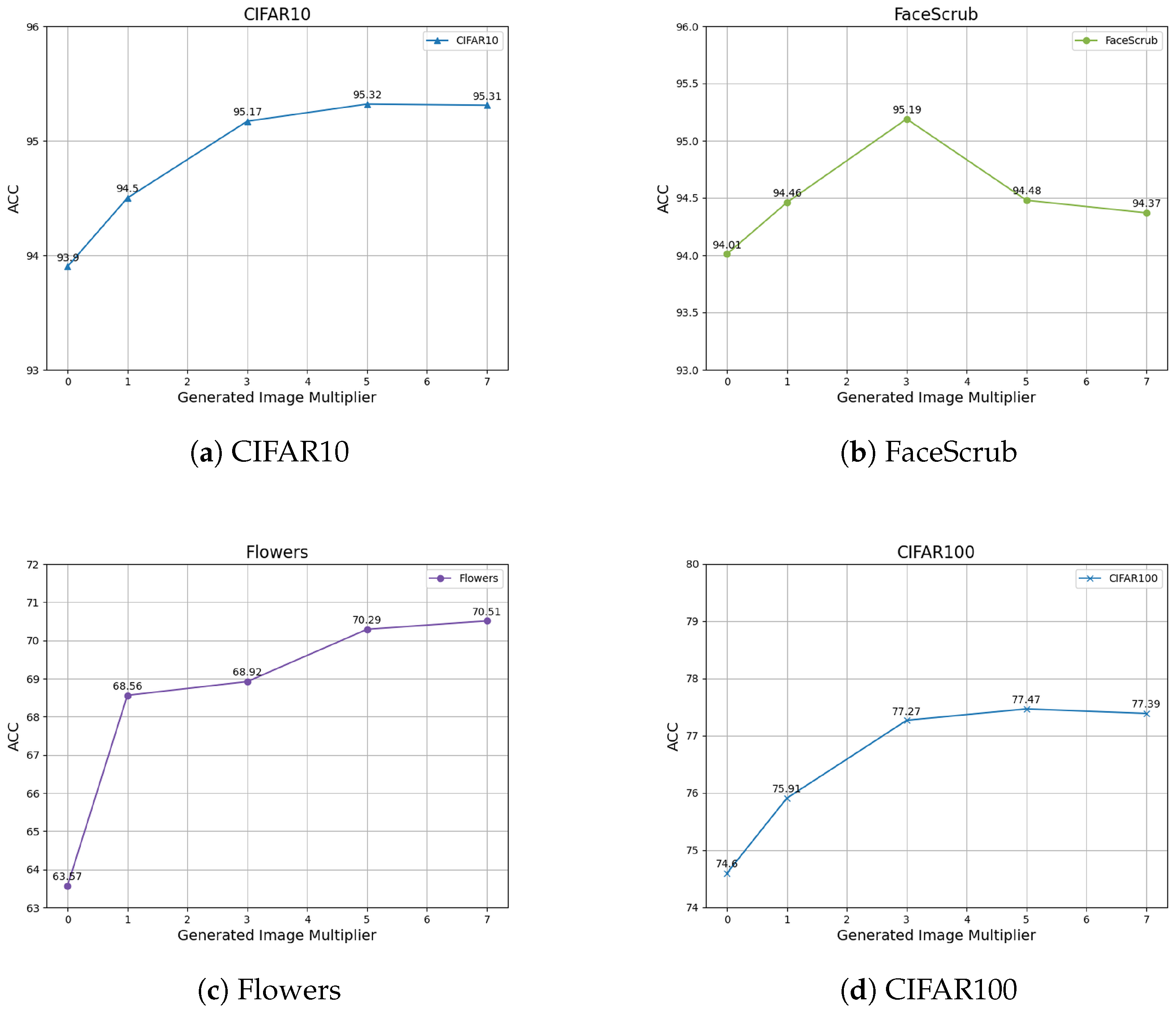
Data augmentation is a key technique to improve model generalization. Research has shown that using generated data for augmentation can enhance performance, but the relationship between the quantity of generated images and accuracy is not extensively discussed. We analyze the effectiveness of using varying quantities of generated images for data augmentation and compare it with the mixup method. As shown in Table 8 and Figure 7, adding multiples of generated data to the original training set can further boost the classification network’s performance, often achieving superior results to mixup. However, the performance curves show that classification performance does not increase indefinitely; inflection points appear at different multiples for different datasets, indicating that an excessive number of generated images can have adverse effects, such as overfitting.

4.4. Ablation Studies

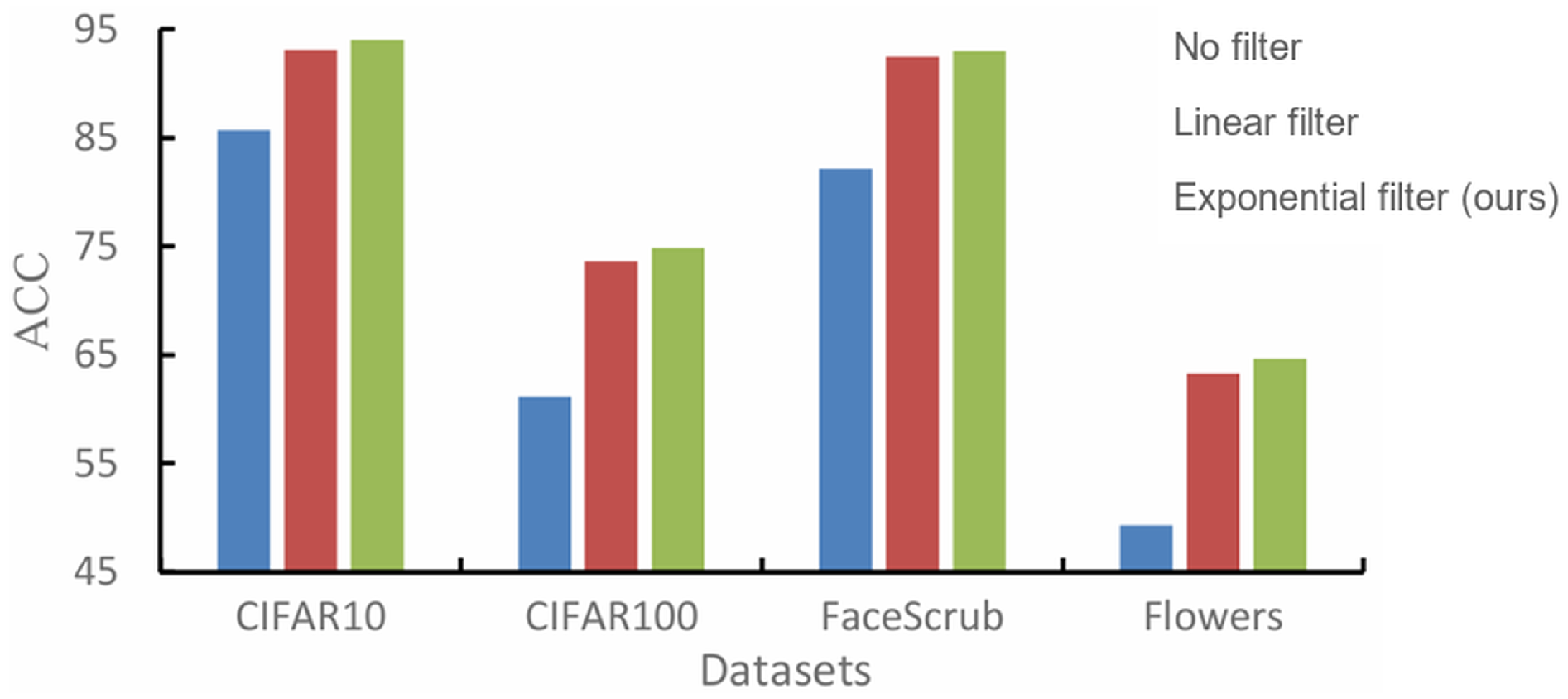
Effectiveness of Noise Filtering: To validate our noise filtering mechanism, we compare the classification performance of CoDC with exponential filtering (our default method), a linear filtering baseline, and no filtering. As shown in Table 9 and Figure 8 and Figure 9, without any filtering, the noise severely pollutes the features, leading to poor accuracy (e.g., 61.14% on CIFAR-100). Linear filtering improves the results, but our proposed exponential filtering, which more accurately models the noise schedule, yields the best performance. This behavior is consistent with the diffusion formulation in Section 3.2: the useful semantic signal retained in x t is controlled by α ¯ t , which decays multiplicatively rather than linearly as the timestep increases. Without filtering, all timesteps contribute equally to L c l a s s i f y , so heavily corrupted samples produce classification gradients that are weakly related to object semantics and can force the classifier branch to learn noise-dominated representations. Linear filtering reduces this problem, but its slow decay still assigns relatively large weights to medium and high noise timesteps where class evidence has already been substantially degraded. By contrast, the exponential rule follows the rapid decay pattern of α ¯ t more closely: it preserves strong supervision from low-noise samples, sharply suppresses semantically ambiguous high-noise samples, and therefore better matches the signal-to-noise ratio seen by the shared UNet encoder. The empirical gaps support this interpretation. Compared with no filtering, exponential filtering improves accuracy by 13.73, 10.85, and 15.36 percentage points on CIFAR-100, FaceScrub, and Flowers, respectively. Compared with linear filtering, it further improves accuracy by 1.26, 0.48, and 1.35 percentage points, showing that the gain is not only due to down-weighting noise in general but also to matching the nonlinear noise accumulation process.
Ablation on Model Depth and Parameter Freezing: We analyze two key design choices: the depth of the UNet encoder and our two-step parameter freezing strategy. Table 10 shows that increasing the number of residual blocks in the UNet encoder from 2 to 3 improves classification performance across datasets, justifying our architectural enhancement. A fourth residual block gives additional gains on CIFAR-100 and Flowers and a marginal gain on FaceScrub, but the default model uses three residual blocks per stage to balance accuracy and model complexity. Table 11 demonstrates the effectiveness of parameter freezing. In the collaborative training setting, freezing the deep encoder layers prevents the degradation of classification ability, improving accuracy by 0.78% on CIFAR-100. This result supports our strategy for mitigating the conflict between the generation and classification tasks.
Effectiveness of Sample Selection: We also analyze the impact of our two-step sample selection strategy. Table 12 shows the results. Without any filtering, performance is limited by the quality of the generated data. Applying only filtering based on confidence improves accuracy by removing semantically ambiguous samples. The full strategy, combining both confidence and feature consistency filtering, yields the best results, improving accuracy by 2.68%, 0.94%, and 3.43% on CIFAR-100, FaceScrub, and Flowers respectively, compared to no selection. This result supports the effectiveness of filtering out deceptive samples with high confidence.

5. Discussion

The results show that CoDC is most appropriate for rehearsal-free CIL settings where storing real old class images is undesirable because of privacy, storage, or deployment constraints. Under the strict rehearsal-free comparison, the method improves over zero-memory baselines without pre-training by replacing real exemplar storage with generated replay and by filtering generated samples before they are reused for incremental learning.
The comparison with methods that use memory should be interpreted carefully. In Table 3 and Table 4, several baselines use a 4% real sample memory buffer, whereas CoDC stores no real old class samples. These tables therefore provide a mixed memory reference comparison rather than a strictly identical protocol. The strict rehearsal-free comparison is reported in Table 5 and Table 6, where all methods use zero memory. Recent large pre-trained model methods in Table 7 are also separated into Group B because they rely on external pre-training and substantially larger backbone capacity.
There are still limitations. First, CoDC depends on the quality and class consistency of generated replay samples, so classes with subtle visual differences may require stronger filtering or better generative modeling. Second, diffusion sampling is more expensive than storing a small memory buffer, even though it avoids retaining private historical images. Third, the reported comparison with recent published baselines is protocol aware but not fully unified across all task splits and backbones. Future work will focus on accelerating replay sampling, improving sample selection, and rerunning more recent baselines under exactly matched class order, initialization, and backbone settings.

6. Conclusions

In this paper, we introduced the Co-Diffusion Classifier (CoDC), a framework for class-incremental learning that unifies image generation and classification within a single diffusion model. The collaborative network does not require an additional classifier, reducing model redundancy and training overhead. By using a dual task architecture with exponential noise filtering and a base task classification pre-training stage followed by collaborative training with parameter freezing, CoDC performs both tasks while mitigating task conflict and noise contamination. We also investigated the use of generated images for data augmentation and observed that an optimal quantity exists because excessive synthetic data can reduce accuracy. In incremental learning, our rehearsal-free generative replay strategy, enhanced by a two-step sample selection process, mitigates catastrophic forgetting without storing any real data from past tasks. Under the strict zero memory setting, CoDC outperforms the compared baselines without pre-training by a large margin. For example, in Scenario 1 on CIFAR-100, CoDC improves accuracy from 35.20% for LwF to 65.97%, corresponding to a 30.77 percentage point gain, and reduces forgetting from 46.56% to 10.11%. In the mixed-protocol reference comparison, CoDC is also 2.05 percentage points higher than the strongest conventional memory-based baseline on CIFAR-100 despite storing no real old class images. In Scenario 2, CoDC reaches 65.50% accuracy on CIFAR-100, compared with 24.12% for LwF, yielding a 41.38 percentage point improvement under the zero memory protocol. In the corresponding mixed-protocol reference table, CoDC is 2.04 percentage points higher than the strongest memory-based baseline on CIFAR-100. These results indicate that filtered generated replay can be a practical alternative to real exemplar storage when privacy or storage constraints prevent rehearsal.

Author Contributions

Conceptualization, J.C. and J.W.; methodology, J.C. and J.W.; software, J.W. and S.W.; validation, J.C., J.W., and S.W.; formal analysis, J.W. and S.W.; investigation, S.W.; resources, J.C.; data curation, Q.Z.; writing—original draft preparation, J.W. and S.W.; writing—review and editing, J.W. and S.W.; visualization, Q.Z.; supervision, J.C.; project administration, J.C. All authors have read and agreed to the published version of the manuscript.

Funding

This research received no external funding.

Institutional Review Board Statement

Not applicable.

Informed Consent Statement

Not applicable.

Data Availability Statement

The datasets analyzed during the current study are publicly available benchmarks, including CIFAR-100 [37], FaceScrub [38], and Flowers-102 [39].

Acknowledgments

During the revision of this manuscript, the authors used an AI-based language tool only for grammar checking, wording refinement, and style polishing. The authors reviewed and edited all content and take full responsibility for the final manuscript.

Conflicts of Interest

The authors declare no conflicts of interest.

Abbreviations

The following abbreviations are used in this manuscript:
CILClass-Incremental Learning
CoDCCo-Diffusion Classifier
CUDACompute Unified Device Architecture
DDIMDenoising Diffusion Implicit Models
DERDynamically Expandable Representation
GRGenerative Replay
FIDFréchet Inception Distance
GANGenerative Adversarial Network
GPUGraphics Processing Unit
MSEMean Squared Error
PTMPre-Trained Model
UNetU-shaped Network

References

  1. Gomes, H.M.; Barddal, J.P.; Enembreck, F.; Bifet, A. A Survey on Ensemble Learning for Data Stream Classification. ACM Comput. Surv. 2017, 50, 1–36. [Google Scholar] [CrossRef] [Scilit]
  2. Krempl, G.; Žliobaite, I.; Brzeziński, D.; Hüllermeier, E.; Last, M.; Lemaire, V.; Stefanowski, J. Open challenges for data stream mining research. ACM SIGKDD Explor. Newsl. 2014, 166, 1–10. [Google Scholar] [CrossRef] [Scilit]
  3. Delange, M.; Aljundi, R.; Masana, M.; Parisot, S.; Jia, X.; Leonardis, A.; Slabaugh, G.; Tuytelaars, T. A continual learning survey: Defying forgetting in classification tasks. IEEE Trans. Pattern Anal. Mach. Intell. 2021, 44, 3366–3385. [Google Scholar] [CrossRef] [Scilit] [PubMed]
  4. Zhu, F.; Zhang, X.Y.; Liu, C.L. Survey and performance evaluation of class-incremental learning. Acta Autom. Sin. 2023, 49, 635–660. [Google Scholar]
  5. Masana, M.; Liu, X.; Twardowski, B.; Menta, M.; Bagdanov, A.D.; van de Weijer, J. Class-incremental learning: Survey and performance evaluation on image classification. IEEE Trans. Pattern Anal. Mach. Intell. 2023, 45, 5513–5533. [Google Scholar] [CrossRef] [Scilit] [PubMed]
  6. Wang, L.; Zhang, X.; Su, H.; Zhu, J. A comprehensive survey of continual learning: Theory, method and application. IEEE Trans. Pattern Anal. Mach. Intell. 2024, 46, 5362–5383. [Google Scholar] [CrossRef] [Scilit] [PubMed]
  7. van de Ven, G.M.; Tuytelaars, T.; Tolias, A.S. Three types of incremental learning. Nat. Mach. Intell. 2022, 4, 1185–1197. [Google Scholar] [CrossRef] [Scilit] [PubMed]
  8. McCloskey, M.; Cohen, N.J. Catastrophic interference in connectionist networks: The sequential learning problem. In Psychology of Learning and Motivation; Academic Press: New York, NY, USA, 1989; pp. 109–165. [Google Scholar]
  9. Parisi, G.I.; Kemker, R.; Part, J.L.; Kanan, C.; Wermter, S. Continual lifelong learning with neural networks: A review. Neural Netw. 2019, 113, 54–71. [Google Scholar] [CrossRef] [Scilit] [PubMed]
  10. Kirkpatrick, J.; Pascanu, R.; Rabinowitz, N.; Veness, J.; Desjardins, G.; Rusu, A.A.; Milan, K.; Quan, J.; Ramalho, T.; Grabska-Barwinska, A.; et al. Overcoming catastrophic forgetting in neural networks. Proc. Natl. Acad. Sci. USA 2017, 114, 3521–3526. [Google Scholar] [CrossRef] [Scilit] [PubMed]
  11. Li, Z.; Hoiem, D. Learning without forgetting. IEEE Trans. Pattern Anal. Mach. Intell. 2018, 40, 2935–2947. [Google Scholar] [CrossRef] [Scilit] [PubMed]
  12. Hayes, T.L.; Krishnan, G.P.; Bazhenov, M.; Siegelmann, H.T.; Sejnowski, T.J.; Kanan, C. Replay in deep learning: Current approaches and missing biological elements. Neural Comput. 2021, 33, 2908–2950. [Google Scholar] [CrossRef] [Scilit] [PubMed]
  13. Graffieti, L.; Maltoni, D.; Pellegrini, D.; Lomonaco, V. Generative negative replay for continual learning. Neural Netw. 2023, 162, 369–383. [Google Scholar] [CrossRef] [Scilit] [PubMed]
  14. Hinton, G.; Vinyals, O.; Dean, J. Distilling the knowledge in a neural network. arXiv 2015, arXiv:1503.02531. [Google Scholar] [CrossRef] [Scilit]
  15. Rebuffi, S.-A.; Kolesnikov, A.; Sperl, G.; Lampert, C.H. iCaRL: Incremental classifier and representation learning. In Proceedings of the IEEE/CVF Conference on Computer Vision and Pattern Recognition (CVPR), Honolulu, HI, USA, 21–26 July 2017; pp. 2001–2010. [Google Scholar]
  16. Rios, A.; Itti, L. Closed-loop memory GAN for continual learning. In Proceedings of the 28th International Joint Conference on Artificial Intelligence (IJCAI), Macao, China, 10–16 August 2019; pp. 3332–3338. [Google Scholar]
  17. Ven, G.M.v.; Siegelmann, H.T.; Tolias, A.S. Brain-inspired replay for continual learning with artificial neural networks. Nat. Commun. 2020, 11, 4069. [Google Scholar] [CrossRef] [Scilit] [PubMed]
  18. Meng, Z.; Zhang, J.; Yang, C.; Zhan, Z.; Zhao, P.; Wang, Y. Diffclass: Diffusion-based class incremental learning. In Proceedings of the European Conference on Computer Vision (ECCV), Milan, Italy, 29 September–4 October 2024; pp. 142–159. [Google Scholar]
  19. Jodelet, Q.; Liu, X.; Phua, Y.J.; Murata, T. Class-incremental learning using diffusion model for distillation and replay. In Proceedings of the IEEE/CVF International Conference on Computer Vision (ICCV), Paris, France, 2–3 October 2023; pp. 3425–3433. [Google Scholar]
  20. Yan, S.; Xie, J.; He, X. DER: Dynamically expandable representation for class incremental learning. In Proceedings of the IEEE/CVF Conference on Computer Vision and Pattern Recognition (CVPR), Virtual, 19–25 June 2021; pp. 3014–3023. [Google Scholar]
  21. Petit, G.; Popescu, A.; Schindler, H.; Picard, D.; Delezoide, B. FeTrIL: Feature translation for exemplar-free class-incremental learning. In Proceedings of the IEEE/CVF Winter Conference on Applications of Computer Vision (WACV), Waikoloa, HI, USA, 3–7 January 2023; pp. 3911–3920. [Google Scholar]
  22. Rypeść, G.; Cygert, S.; Khan, V.; Trzciński, T.; Zieliński, B.; Twardowski, B. Divide and not forget: Ensemble of selectively trained experts in Continual Learning. In Proceedings of the International Conference on Learning Representations (ICLR), Vienna, Austria, 7–11 May 2024. [Google Scholar]
  23. He, R.; Fang, D.; Xu, Y.; Cui, Y.; Li, M.; Chen, C.; Zeng, Z.; Zhuang, H. Semantic shift estimation via dual-projection and classifier reconstruction for exemplar-free class-incremental learning. In Proceedings of the 42nd International Conference on Machine Learning (ICML), PMLR, Vancouver, BC, Canada, 13–19 July 2025; Volume 267, pp. 22392–22406. [Google Scholar]
  24. Abbasnejad, E.; Gong, D.; McDonnell, M.D.; Parvaneh, A.; Hengel, A.V.D. RanPAC: Random projections and pre-trained models for continual learning. In Proceedings of the Advances in Neural Information Processing Systems (NeurIPS), New Orleans, LA, USA, 10–16 December 2023; Volume 36. [Google Scholar]
  25. Zhou, D.-W.; Zhang, Y.; Ye, H.-J.; Zhan, D.-C.; Liu, Z. Expandable subspace ensemble for pre-trained model-based class-incremental learning. In Proceedings of the IEEE/CVF Conference on Computer Vision and Pattern Recognition (CVPR), Seattle, WA, USA, 16–22 June 2024. [Google Scholar]
  26. Wang, Y.; Zhou, D.W.; Ye, H.J. Integrating task-specific and universal adapters for pre-trained model-based class-incremental learning. In Proceedings of the IEEE/CVF International Conference on Computer Vision (ICCV), Honolulu, HI, USA, 19–23 October 2025. [Google Scholar]
  27. Qiu, H.; Zhang, M.; Qiao, Z.; Guan, W.; Zhang, M.; Nie, L. SplitLoRA: Balancing stability and plasticity in continual learning through gradient space splitting. In Proceedings of the International Conference on Learning Representations (ICLR), Rio de Janeiro, Brazil, 27–28 August 2026. [Google Scholar]
  28. Ho, J.; Jain, A.; Abbeel, P. Denoising diffusion probabilistic models. In Proceedings of the Advances in Neural Information Processing Systems (NeurIPS), Virtual, 6–12 December 2020; pp. 6840–6851. [Google Scholar]
  29. Croitoru, F.-A.; Hondru, V.; Ionescu, R.T.; Shah, M. Diffusion models in vision: A survey. IEEE Trans. Pattern Anal. Mach. Intell. 2023, 45, 10850–10869. [Google Scholar] [CrossRef] [Scilit] [PubMed]
  30. Yang, L.; Zhang, Z.; Song, Y.; Hong, S.; Xu, R.; Zhao, Y.; Zhang, W.; Cui, B.; Yang, M.-H. Diffusion models: A comprehensive survey of methods and applications. ACM Comput. Surv. 2023, 56, 1–39. [Google Scholar] [CrossRef] [Scilit]
  31. Ronneberger, O.; Fischer, P.; Brox, T. U-net: Convolutional networks for biomedical image segmentation. In Proceedings of the Medical Image Computing and Computer-Assisted Intervention (MICCAI), Munich, Germany, 5–9 October 2015; pp. 234–241. [Google Scholar]
  32. Song, J.; Meng, C.; Ermon, S. Denoising diffusion implicit models. arXiv 2020, arXiv:2010.02502. [Google Scholar]
  33. Rombach, R.; Blattmann, A.; Lorenz, D.; Esser, P.; Ommer, B. High-resolution image synthesis with latent diffusion models. In Proceedings of the IEEE/CVF Conference on Computer Vision and Pattern Recognition (CVPR), New Orleans, LA, USA, 18–24 June 2022; pp. 10684–10695. [Google Scholar]
  34. Schneider, F. Archisound: Audio generation with diffusion. arXiv 2023, arXiv:2301.13267. [Google Scholar] [CrossRef] [Scilit]
  35. Poole, B.; Jain, A.; Barron, J.T.; Mildenhall, B. Dreamfusion: Text-to-3d using 2d diffusion. arXiv 2022, arXiv:2209.14988. [Google Scholar]
  36. Zhu, Q.; Zu, X. A softmax-free loss function based on predefined optimal-distribution of latent features for deep learning classifier. IEEE Trans. Circuits Syst. Video Technol. 2022, 33, 1386–1397. [Google Scholar] [CrossRef] [Scilit]
  37. Krizhevsky, A.; Hinton, G. Learning Multiple Layers of Features from Tiny Images; Technical Report; University of Toronto: Toronto, ON, Canada, 2009. [Google Scholar]
  38. Ng, H.W.; Winkler, S. A data-driven approach to cleaning large face datasets. In Proceedings of the 2014 IEEE International Conference on Image Processing (ICIP), Paris, France, 27–30 October 2014; pp. 343–347. [Google Scholar]
  39. Nilsback, M.E.; Zisserman, A. Automated flowers classification over a large number of classes. In Proceedings of the Sixth Indian Conference on Computer Vision, Graphics and Image Processing (ICVGIP), Bhubaneswar, India, 16–19 December 2008; pp. 722–729. [Google Scholar]
  40. Heusel, M.; Ramsauer, H.; Unterthiner, T.; Nessler, B.; Hochreiter, S. GANs trained by a two time-scale update rule converge to a local nash equilibrium. In Proceedings of the Advances in Neural Information Processing Systems (NeurIPS), Long Beach, CA, USA, 4–9 December 2017. [Google Scholar]
  41. Wang, F.-Y.; Zhou, D.-W.; Ye, H.-J.; Zhan, D.-C. Foster: Feature boosting and compression for class-incremental learning. In Proceedings of the European Conference on Computer Vision (ECCV), Tel Aviv, Israel, 23–27 October 2022; pp. 398–414. [Google Scholar]
  42. Zhou, D.W.; Wang, Q.W.; Ye, H.J.; Zhan, D.C. A model or 603 exemplars: Towards memory-efficient class-incremental learning. In Proceedings of the International Conference on Learning Representations (ICLR), Virtually, 1–5 May 2023. [Google Scholar]
  43. Zhu, K.; Zhai, W.; Cao, Y.; Luo, J.; Zha, Z.-J. Self-sustaining representation expansion for non-exemplar class-incremental learning. In Proceedings of the IEEE/CVF Conference on Computer Vision and Pattern Recognition (CVPR), New Orleans, LA, USA, 18–24 June 2022; pp. 9296–9305. [Google Scholar]
Figure 1. Comparison between traditional generative replay and the proposed CoDC framework in streaming class-incremental learning. (a) Conventional generative replay uses a cascaded pipeline in which a separate generator synthesizes replay samples and a separate classifier is then updated with the mixed data. This separation increases training overhead and can propagate semantic bias from generated samples. (b) CoDC unifies replay generation, replay sample filtering, and classification in one diffusion-based network. The shared encoder provides features for the classifier head, the decoder generates old class replay candidates, and the filtered generated samples are merged with current task data for joint updating without storing real old class images.
Applsci 16 06035 g001
Figure 2. The proposed dual task architecture for the UNet. The standard generative path is optimized with L m s e . A classification head is attached to an intermediate encoder layer and optimized with L c l a s s i f y , enabling simultaneous generation and classification.
Applsci 16 06035 g002
Figure 3. The relationship between α ¯ t and time t. The red line (exact value) shows a strong correlation with the blue dashed line ( t 2 term).
Applsci 16 06035 g003
Figure 4. Default exponential noise filtering used by CoDC. The weight coefficient decreases exponentially as the timestep t increases, focusing the classifier’s training on less noisy samples.
Applsci 16 06035 g004
Figure 5. Complete pipeline of CoDC for rehearsal-free streaming class-incremental learning. At task k, the previous model CoDC k 1 receives old class labels as conditioning information and generates old class replay candidates by DDIM sampling. These candidates are filtered by classification confidence and feature consistency with stored class feature prototypes μ c , which are compact feature statistics rather than stored images. The retained replay samples are merged with real samples from the current task to form the mixed training batch used to update CoDC k with the collaborative objective; Stage 1 classification pre-training is only used for the base task. After the update, CoDC k is carried forward as the previous model for task k + 1 , while real samples from past tasks are not stored.
Applsci 16 06035 g005
Figure 6. Sample comparison on CIFAR-100 (apples). (a) shows original images. (b) shows raw generated images, including blurry or label ambiguous cases. (c) shows samples retained after confidence and feature filtering, which are more consistent with the target label for replay.
Applsci 16 06035 g006
Figure 7. Relationship between classification accuracy and the quantity of generated images used for data augmentation. The x-axis represents the multiple of generated images relative to the base training set size (0 means base set only). Performance generally improves but then plateaus or declines, indicating an optimal amount of synthetic data.
Applsci 16 06035 g007
Figure 8. Linear noise filtering baseline used only for ablation. The weight coefficient decreases linearly as the timestep t increases.
Applsci 16 06035 g008
Figure 9. Classification accuracy under different noise filtering strategies. No filter uses no timestep weighting, linear filter is the ablation baseline, and exponential filter is the default CoDC strategy.
Applsci 16 06035 g009
Table 1. Classification and generation performance of CoDC.
MetricModelCIFAR-100FaceScrubFlowers
ACC (%)Specialist74.6094.0163.57
CoDC (Ours, exponential filter)74.8792.9564.66
FIDSpecialist5.325.2724.70
CoDC (Ours)5.485.1025.10
Table 2. Classification performance of data generated by original and collaborative networks.
Generated Data SourceCIFAR-100FaceScrubFlowers
Collaborative Network66.4386.5854.10
Original Network67.8885.4355.20
Table 3. Mixed-protocol reference comparison: final accuracy (%) with 20 base classes and 20-class steps (baselines use 4% real-sample memory; CoDC uses 0 memory).
MethodCIFAR-100FaceScrubFlowers
ICaRL(NME) [15]54.2880.3927.30
Foster(CNN) [41]59.4466.3029.10
DER(CNN) [20]63.9290.4334.80
MEMO(CNN) [42]62.2980.9832.00
CoDC (Ours, 0 memory)65.9780.5055.30
Table 4. Mixed-protocol reference comparison: final accuracy (%) with 50 base classes and 10-class steps (baselines use 4% real-sample memory; CoDC uses 0 memory).
MethodCIFAR-100FaceScrubFlowers
ICaRL(NME) [15]51.5779.4933.10
Foster(CNN) [41]58.7776.4634.50
DER(NME) [20]63.4690.2046.90
MEMO(NME) [42]58.7460.6528.10
CoDC (Ours, 0 memory)65.5080.1653.73
Table 5. Rehearsal-free setting (0 memory) comparison—Scenario 1 (20 base, 20-class steps).
CIFAR-100FaceScrubFlowers
MethodAccuracy (%)Forgetting (%)Accuracy (%)Forgetting (%)Accuracy (%)Forgetting (%)
ICaRL(CNN) [15]17.5382.1718.6393.0516.3076.20
DER(CNN) [20]15.9282.2519.1794.6716.4074.53
MEMO(CNN) [42]17.0184.0718.8492.9517.3075.91
LwF(CNN) [11]35.2046.5640.8653.1433.6039.99
Ours65.9710.1180.5013.9755.3022.86
Table 6. Rehearsal-free setting (0 memory) comparison—Scenario 2 (50 base, 10-class steps).
CIFAR-100FaceScrubFlowers
MethodAccuracy (%)Forgetting (%)Accuracy (%)Forgetting (%)Accuracy (%)Forgetting (%)
ICaRL(CNN) [15]8.9483.189.3495.457.6076.40
DER(CNN) [20]8.5780.659.7895.588.9075.93
MEMO(CNN) [42]8.4983.259.5593.168.5078.81
LwF(CNN) [11]24.1237.8327.5739.8318.4034.21
Ours65.508.7880.1610.0253.7318.58
Table 7. Protocol aware comparison with recent rehearsal-free and pre-trained model-based CIL methods on CIFAR-100. Direct comparison is intended only within Group A. Group B is included to position CoDC relative to recent large pre-trained model results, not to rank methods under the same computational setting.
MethodVenueSetting/SourceBackbone or Pre-TrainingAvg. Acc. (%)Final Acc. (%)
Group A: Standard methods without large external pre-training (direct comparison)
LwF [11]TPAMI’17Ours, 20-class stepsResNet-3235.20
ABD (reported in [18])ICCV’21DiffClass, N = 5, memory = 0ResNet-1860.7844.69
PASS (reported in [18])CVPR’21DiffClass, N = 5, memory = 0ResNet-1863.3149.27
IL2A (reported in [18])NeurIPS’21DiffClass, N = 5, memory = 0ResNet-1858.6744.96
R-DFCIL (reported in [18])ECCV’22DiffClass, N = 5, memory = 0ResNet-1864.6749.48
SSRE [43]CVPR’22DiffClass, N = 5, memory = 0ResNet-1856.9639.89
FeTrIL [21]WACV’23DiffClass, N = 5, memory = 0ResNet-1858.6842.67
SEED [22]ICLR’24DiffClass, N = 5, memory = 0ResNet-1863.0552.14
DPCR [23]ICML’25Authors’ CIFAR-100, 10 tasksResNet-1863.2150.24
CoDC (Ours)Ours, 20-class stepsUNet65.9757.21
Group B: Pre-trained large-model methods (reference only)
DiffClass [18]ECCV’24DiffClass, N = 5, memory = 0Stable Diffusion v1.5 + LoRA69.7762.21
L2P (reported in [25])CVPR’22EASE, B0 Inc5 PTM settingViT-B/16-IN21K85.9479.93
DualPrompt (reported in [25])ECCV’22EASE, B0 Inc5 PTM settingViT-B/16-IN21K87.8781.15
CODA-Prompt (reported in [25])CVPR’23EASE, B0 Inc5 PTM settingViT-B/16-IN21K89.1181.96
SimpleCIL (reported in [25])CVPR’24EASE, B0 Inc5 PTM settingViT-B/16-IN21K87.5781.26
ADAM+Adapter (reported in [25])CVPR’24EASE, B0 Inc5 PTM settingViT-B/16-IN21K90.6585.15
EASE [25]CVPR’24EASE, B0 Inc5 PTM settingViT-B/16-IN21K91.5185.80
TUNA [26]ICCV’25Authors’ B0 Inc5 PTM settingViT-B/16-IN21K94.4490.74
SplitLoRA [27]ICLR’26Authors’ B0 Inc5 PTM settingViT-B/16-IN21K93.1190.84
Avg. Acc. denotes average incremental accuracy. Final Acc. denotes the last-stage accuracy when reported. Rows marked “reported in” reuse published comparison tables rather than rerunning the methods. Because task splits, initialization, and backbones are not identical across sources, Group A is used for protocol aware comparison and Group B is reference only.
Table 8. Data augmentation effects of generated images and mixup (accuracy %).
MethodCIFAR10CIFAR100FaceScrubFlowers
base93.9774.6094.0163.57
mixup95.3077.3695.1765.20
ddim250 × 191.0367.8885.4355.20
ddim250 × 393.7074.0388.7363.86
ddim250 × 594.2675.8589.8466.83
base+ddim250 × 194.5075.9194.4668.56
base+ddim250 × 395.1777.2795.1968.92
base+ddim250 × 595.3277.4794.4870.29
base+ddim250 × 795.3177.3994.3770.51
Table 9. Ablation study on noise filtering mechanism (accuracy %).
Filter TypeCIFAR-100FaceScrubFlowers
No Filter61.1482.1049.30
Linear Filter73.6192.4763.31
Exponential (Ours)74.8792.9564.66
Table 10. Ablation study on UNet encoder depth (accuracy %).
Blocks per StageCIFAR-100FaceScrubFlowers
274.6094.0163.57
3 (default)75.1594.2065.25
476.5294.2165.74
Table 11. Ablation study on parameter freezing (accuracy %).
StrategyCIFAR-100FaceScrub
No Freezing65.5080.16
With Freezing (Ours)66.2880.25
Table 12. Ablation study on generated sample selection (accuracy %).
Selection StrategyCIFAR-100FaceScrubFlowers
No Selection63.2979.5651.87
Confidence Only65.6680.2954.86
Confidence + Feature65.9780.5055.30
Disclaimer/Publisher’s Note: The statements, opinions and data contained in all publications are solely those of the individual author(s) and contributor(s) and not of MDPI and/or the editor(s). MDPI and/or the editor(s) disclaim responsibility for any injury to people or property resulting from any ideas, methods, instructions or products referred to in the content.