Article

Research on a Tracking Control Method Assisted by Visual Targets in the Autonomous Navigation Task of a Split Drilling Robot


1
School of Mechatronic Engineering, China University of Mining and Technology, Xuzhou 221116, China
2
School of Information and Control Engineering, China University of Mining and Technology, Xuzhou 221116, China
3
Jiangsu Collaborative Innovation Center of Intelligent Mining Equipment, China University of Mining and Technology, Xuzhou 221008, China
*
Author to whom correspondence should be addressed.
Appl. Sci. 2026, 16(12), 5929; https://doi.org/10.3390/app16125929
Submission received: 10 May 2026 / Revised: 5 June 2026 / Accepted: 8 June 2026 / Published: 11 June 2026
(This article belongs to the Topic Fuzzy Optimization and Decision Making)

Abstract

Split-type robots are increasingly deployed in unstructured confined environments such as underground coal mines, where autonomous navigation and cooperative tracking control remain critical challenges. This paper presents a visual target-assisted tracking control scheme for a split-type drilling robot, adopting an active leader–passive follower architecture. The leader robot performs autonomous mobility and obstacle avoidance using 3D LiDAR-based offline path generation and online optimal search. The follower robot uses AprilTag visual fiducial markers to estimate the six-degree-of-freedom relative pose via the Perspective-N-Point algorithm, and it tracks the leader using a two-dimensional fuzzy PID controller that adaptively tunes PID parameters. Extensive experiments are conducted in simulation, simulated tunnels, a large-scale robot platform, and a real drilling robot prototype. Results demonstrate that the leader achieves an average navigation error below 0.175 m, while the follower maintains an average relative tracking error within 0.06 m. The proposed method enables stable, comparable accuracy with smoother, less oscillatory response, and high-precision cooperative navigation for heavy-duty split-type robots, offering a practical solution for intelligent drilling operations in underground confined spaces.

1. Introduction

Split-type robots represent one of the most active research areas in current robotics. They are autonomous unmanned systems integrating sensor technology, control theory, and intelligent algorithms, and they are widely used to perceive unstructured task environments, make autonomous decisions, and complete both daily tasks and high-risk operations. Compared with traditional robots, split-type robots decompose a complex, high-difficulty, high-risk overall system into multiple individual units, each dedicated to a single task. This reduces maintenance difficulty, decreases the robot’s physical footprint, and improves adaptability to complex working conditions. They have been widely deployed in confined spaces such as search and rescue [1], shaft maintenance [2], pipeline inspection [3], and medical surgery [4]. Therefore, split-type robots hold immense development potential in the current era of intelligent technology. For split-type robots to achieve intelligence, the first problems to be solved are perception, navigation, cooperation, and control.
Regarding the perception problem of split-type robots, current research mainly focuses on collaborative mapping and the map merging of robot swarms [5,6]. For the autonomous navigation of split-type robots, the core challenges lie in achieving the independent mobility of each split unit and enabling cooperative control among multiple units. Current path planning for individual robots mainly relies on 3D LiDAR point cloud maps and mathematical models for trajectory optimization [7,8]; swarm navigation is achieved through interaction mechanisms to transmit key navigation information, followed by the execution of individual navigation algorithms once core data are obtained [9,10].
In split-type robot cooperative control scenarios, the follower robot typically relies on visual fiducial markers for precise relative localization. Therefore, the study of visual fiducial marker systems has become an important research topic. In 2011, Edwin Olson proposed AprilTag [11] and its improved version [12], which achieve good localization and detection accuracy in UAV visual tracking tasks. Subsequent research has explored and improved detection accuracy [13], computational efficiency [14], high-speed motion [15], and image modalities [16]. With the rapid development of deep learning, methods using artificial neural networks (ANNs) [17,18] combined with backpropagation training have been developed to estimate six-degree-of-freedom (6-DoF) poses of cameras relative to markers.
For cooperative control between split-type robots, PID control has been widely adopted in industrial applications due to its simple principle, ease of implementation, good real-time performance, and high stability and robustness. Subsequently, sliding mode control algorithms have emerged for nonlinear control models [19], and model predictive control (MPC) methods applicable to both linear and nonlinear models have been developed [20,21]. In robotics, these are mainly applied to trajectory tracking control tasks [22]. With the development of neural networks, neural network-based control algorithms have also appeared [23,24].
In recent years, fuzzy logic control has been widely adopted for the trajectory tracking of mobile robots due to its strong adaptability to nonlinear systems and complex working conditions. Wahyuni et al. [25] adopt a Fuzzy-PID control strategy combined with MPU6050 gyroscope feedback to improve the motion stability and terrain adaptability of four-wheeled mobile robots on horizontal, uphill, and downhill paths. Tolossa et al. [26] optimized the parameters of fuzzy controllers to improve the tracking performance of mobile robots. Hailu et al. [27] conducted comprehensive comparisons among conventional PID, standard fuzzy PID, and optimized fuzzy PID, proving that fuzzy-based strategies obtain better dynamic performance. In addition, Pérez-Juárez et al. [28] designed a kinematic fuzzy controller suitable for wheeled robots with nonholonomic constraints. To further enhance anti-interference capability, Benaicha et al. [29] proposed an improved fuzzy control scheme for robot navigation in unknown environments. Focusing on multi-robot scenarios, He et al. [30] studied trajectory tracking control for cooperative transportation systems. For differential-drive robots, Cosenza et al. [31] developed a virtual sensor to estimate wheel speed, which helps improve the accuracy of robot motion control.
Different from the above studies on ordinary ground robots, this paper designs a two-dimensional fuzzy PID controller specifically for heavy-load hydraulically driven split drilling robots working in underground coal mine environments. Compared with the existing traditional PID control methods, this controller features stronger robustness in trajectory tracking when coping with complex underground coal mine scenarios. It can not only achieve ideal tracking accuracy, but it can also deliver a faster response speed.
In this paper, we take a split-type drilling robot as the research object. To meet the autonomous mobility and obstacle avoidance requirements of split-type robots under real working conditions, we propose a navigation strategy based on active leader–passive follower cooperation. Building on our previous work [32], we focus on the tracking control method assisted by visual fiducial markers for the autonomous navigation task of the split-type drilling robot. The specific contributions of this study are as follows:
  • Based on the structural characteristics of split-type robots, we propose an active leader–passive follower navigation strategy. The leader performs path planning on a 3D LiDAR point cloud map to achieve autonomous mobility and obstacle avoidance. The follower uses AprilTags as visual fiducial markers for localization and tracks the leader visually using a fuzzy PID control algorithm, thereby realizing overall autonomous navigation of the split-type robot.
  • We propose a motion control method for the drilling robot based on fuzzy PID. A two-dimensional fuzzy PID architecture is adopted, and a fuzzy control lookup table is defined, enabling accurate tracking control of the follower to the leader.
  • Experiments on autonomous navigation and tracking control of the split-type robot are carried out in a simulation environment, a simulated tunnel, and on a real drilling robot. The results demonstrate that the proposed method enables the follower to accurately track the autonomously navigating leader.
The structure of this manuscript is arranged as follows. Section 2 describes the system configuration and hardware setup. Section 3 illustrates the path planning strategy for the guiding robot. Section 4 explains the visual pose detection method using AprilTag and PnP technology. Section 5 designs the fuzzy PID controller for follower tracking. Simulation and experimental validations are conducted in Section 6. Section 7 concludes this work and discusses future research.

2. Working Conditions and System Architecture

2.1. Basic Working Conditions and Navigation Requirements of the Split-Type Drilling Robots

Figure 1 shows the physical prototype of the drilling robot used in this study. The drilling robot system adopts a split-type structure, consisting of a leader (front robot) for directional drilling operations and a follower (rear robot) for drill pipe transport. These are heavy-duty tracked mobile platforms with a large aspect ratio, driven by hydraulic differential systems and moving at low speeds. The front robot includes a frame and a power head, primarily responsible for drilling operations. The rear robot comprises a drill pipe magazine and a manipulator, whose main function is to use the robotic arm to retrieve drill pipes from the magazine and deliver them to the designated position, working together with the power head and double clamps to achieve automatic rod feeding, drilling, rod unloading, and retrieval. The robots operate in known unstructured underground roadways, performing long-duration, high-intensity repetitive drilling and drill pipe transport tasks within a local area. During operation, the front robot needs to perform repetitive drilling tasks in a fixed area. Since drilling takes a long time and the moving time is negligible compared to the operating time, achieving autonomous mobility of the front robot is of great significance for saving labor costs. The rear robot, constrained by the length of the robotic arm, must accurately follow the movement of the front robot to ensure timely delivery of drill pipes to the designated position, thereby guaranteeing the efficiency and continuity of the drilling operation.
Different from swarm robots designed for large-scale formation and long-distance cooperative navigation, the split-type drilling robot in this study performs short-range leader–follower tracking in narrow underground roadways. For this specific close-range working scenario, the conventional Simultaneous Localization and Mapping (SLAM)-based autonomous navigation scheme is infeasible for the follower robot. Standard SLAM systems treat moving objects as dynamic obstacles and eliminate them from static mapping. During continuous short-range following, the leader robot always maintains a relatively fixed position and stable relative motion in front of the follower. In this case, the leader is persistently identified as a frontal dynamic obstacle, which eventually leads to navigation failure. To address this inherent limitation of traditional SLAM in close-range cooperative scenarios, this paper proposes a vision-only fiducial tracking strategy for underground split-type robots. The follower achieves stable cooperative tracking relying on visual pose perception, which matches the actual working characteristics of underground narrow roadway environments.
The detailed parameters of the front and rear robots of the drilling robot are listed in Table 1. On the one hand, it drives the mine-used AC servo motor to realize the rotary drive control of the drill bit; on the other hand, it drives the large hydraulic pump unit and hydraulic motor to fulfill the functions of chassis traveling, drill bit lifting and lowering control, and drilling and retracting of the robot. The drilling robot is equipped with an AC/DC transformer inside, which can provide 48 V DC power for the main control computer and PLC controllers.

2.2. Architecture of the Autonomous Navigation System and Visual Tracking System

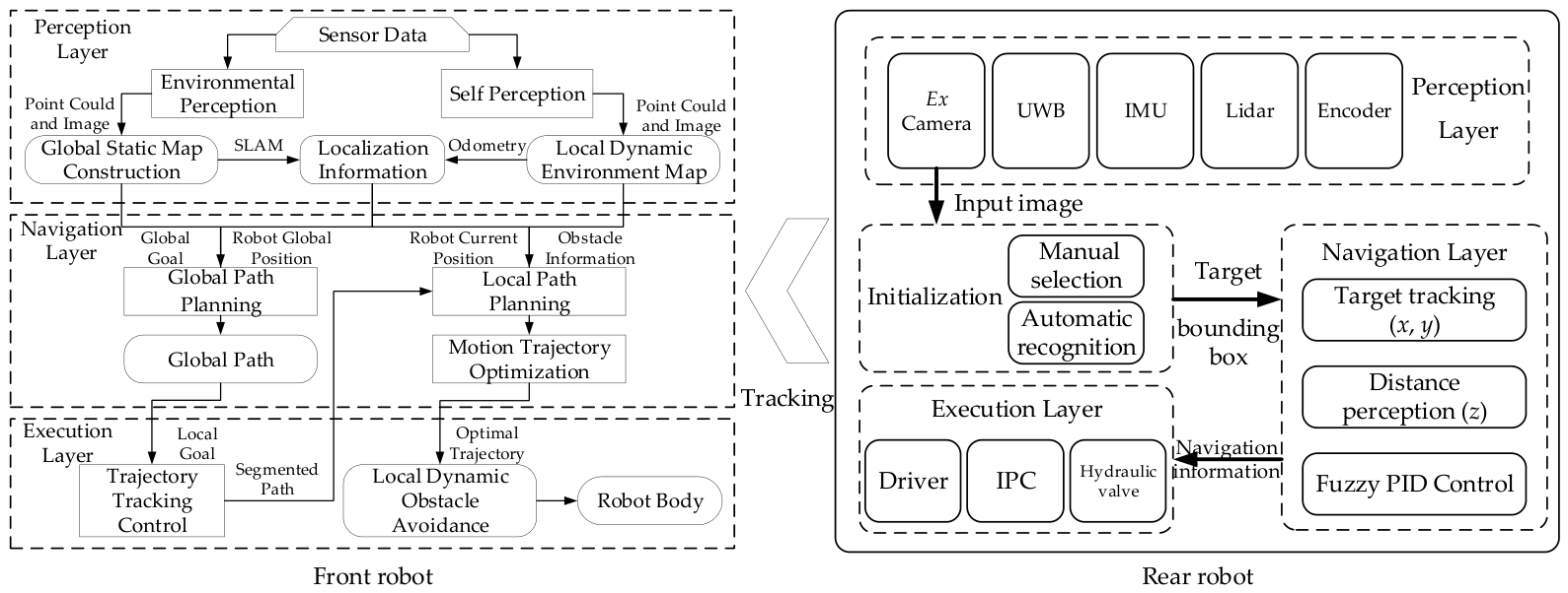
The basic framework of the autonomous navigation and visual tracking system for the split-type coal mine drilling robot is shown in Figure 2. The system is mainly divided into the perception layer, navigation layer, and execution layer. The perception layer consists of an explosion-proof monocular camera, a 3D LiDAR, UWB, IMU, and encoders. Its main function is to process the input information from the perception sensors and generate effective pre-input information for navigation. The front robot uses LiDAR, IMU, an explosion-proof camera, and UWB to perceive the external environment and its own state, while the rear robot uses only a monocular explosion-proof camera to acquire raw images of the target. Other sensor modules of the follower are reserved for its independent autonomous navigation mode and are not used in the research content of this paper. Both robots are equipped with a Nuvo-5095 GC industrial computer as the main control terminal of the autonomous navigation system, featuring an Intel Core i7-6700 CPU and a NVIDIA GTX 1650 Ti GPU with 75 W TDP. It is equipped with 32 Gib DDR4 3200 MHz memory and a 500 Gib M.2 NVME 2280 solid-state drive, with Ubuntu 18.04 as the operating system. To ensure that all perception, planning and tracking algorithms can compute and run in real time at the millisecond level.
The navigation layer of the front robot relies on the map and localization information from the perception layer and includes global path planning, local path planning, and trajectory optimization. Global path planning computes a collision-free guiding path using a static global map. Local path planning generates feasible local trajectories under constraints such as kinematics/dynamics, environmental changes, and terrain. The trajectory optimization module selects the best trajectory from the solution set according to multiple criteria. The execution layer performs kinematic smoothing on the path, converts discrete path points into a time-continuous function, and achieves accurate path tracking and drive control through trajectory tracking control.
For the rear robot, the navigation layer first initializes the tracking target from the images captured by the camera. There are generally two methods: manual selection by framing the target in the operation interface, or automatic target selection using a target recognition algorithm. This paper adopts the second method, i.e., automatic recognition. After confirming the target to be tracked, the visual tracking module in the navigation layer tracks the target to obtain in-plane motion variations. The proposed visual-fiducial-assisted tracking control method is then used to obtain target pose information and output navigation commands such as linear and angular velocities. Finally, the navigation information is sent to the industrial computer in the execution layer (main control system) to control the left and right track hydraulic valves of the follower, thereby achieving tracking of the leader.
The software system uses ROS node communication for interaction. The sensor driver module, target tracking module, SLAM module, and path planning module run independently on the onboard industrial computer. The remote monitoring host can run a visualization interface and send remote control commands. Each functional node and module interacts by subscribing to required topics or making requests. Therefore, when needed, the target tracking node can be turned on or off independently (i.e., depending on whether the rear robot tracking function is required) without affecting other modules.
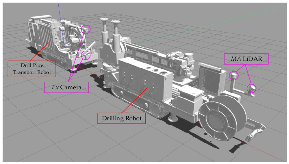
Figure 3 shows the overall system schematic of the drilling robot and the drill pipe transport robot. During drilling operations, the leader (drilling robot) and the follower (drill pipe transport robot) are connected via an armored optical fiber for communication. However, during movement, the cable must be disconnected to prevent it from being pulled apart. Since the feed distance of the follower’s drill pipe can be adaptively adjusted by the manipulator during operation, it is sufficient to ensure that the follower remains within a certain distance range from the leader. Therefore, the tracking system was designed with the assumption that during forward movement, only the leader body is ahead of the follower, the walls on both sides are flush with the obstacles beside the drilling robot, and no new obstacles appear in the area traversed by the leader. This allows the follower to use a navigation system independent of the leader for front–rear robot following, i.e., the follower’s tracking system is responsible only for the follower, and the leader’s navigation system is responsible only for the leader. As long as the following distance between the follower and the leader is within a safe range, the visual following function is considered achieved. No data communication is performed between the two during the following process, thus avoiding occupying communication line bandwidth.

2.3. Selection of Visual Fiducial Markers

Visual fiducial markers are essential for the cooperative tracking of split mining robots, and their environmental adaptability and positioning accuracy directly determine tracking stability in complex underground scenarios. Typical mine environments suffer from uneven illumination, dust interference, image blurring, and partial occlusion, which impose strict requirements on visual detection performance. We compared five mainstream markers in Appendix A, as shown in Table A1, namely, AprilTag, ArUco, ChArUco, ARToolKit, and QR Code. Most conventional markers have obvious limitations: QR codes and ARToolKit lack precise pose-solving capability and anti-interference robustness; ChArUco is unsuitable for dynamic tracking due to its large deployment size and low real-time performance; ArUco is lightweight but susceptible to illumination variation and blurring, resulting in unstable detection in harsh mine environments.
Compared with other markers, AprilTag delivers better overall performance suited for the complex working conditions underground. It maintains stable recognition under conditions such as fluctuating lighting, shadow coverage, dust blurring, and partial occlusion. A single AprilTag marker can realize six-degree-of-freedom pose estimation with millimeter-level positioning accuracy, which meets the core requirement of high-precision tracking for the system. Meanwhile, it is compatible with mainstream robot development frameworks including ROS, featuring flexible on-site deployment and low costs. Therefore, this paper adopts AprilTag as the visual positioning marker for the robot cooperative tracking system.

2.4. Host Computer Interface

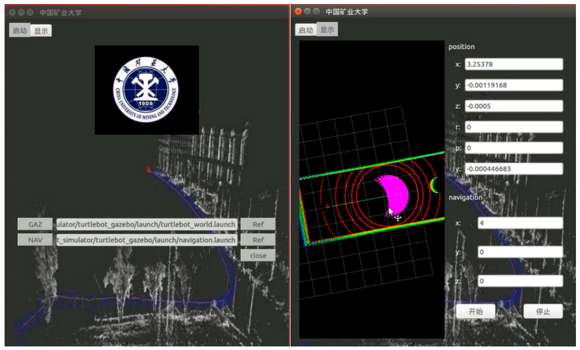
To facilitate human–computer interaction, the host computer interface was designed using Qt 5, as shown in Figure 4. The left side is the startup interface, which includes the selection and launch of Gazebo 9 simulation and navigation files. The right side is the display interface, showing point cloud display, pose display, navigation target point setting and publishing, robot trajectory display, and drivable path display. The interface is designed with a multi-threading approach: the child thread runs ROS-related program modules, subscribes to point cloud topics and robot pose topics, and publishes navigation target points; the main thread refreshes the interface to display point cloud and pose data. Data interaction between the child thread and the main thread uses the signal-slot mechanism of Qt 5. In the figure, the purple line is the drivable path, the green line is the robot trajectory, and the colored points represent the point cloud map.

3. Path Planning and Obstacle Avoidance Method for the Leader Robot

3.1. Path Planning Model

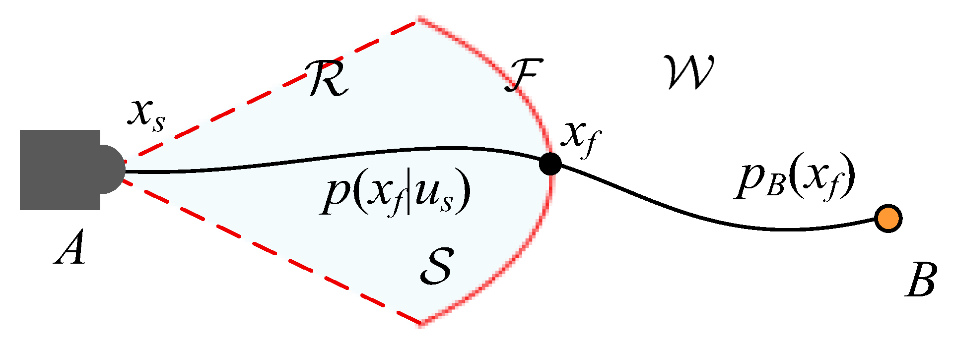
To address the high computational complexity of online path planning, this paper adopts an offline approach that pre-generates traversable paths. Online, the robot selects the best pre-generated path to execute. As shown in a related work [8], the path planning problem can be formulated as a probabilistic model illustrated in Figure 5. Let 𝒲 denote the robot’s motion space, A 𝒲 represent the starting position of the front part of the articulated robot, and B 𝒲 represent the target position the robot needs to reach. Assume the robot carries its own laser sensor; S 𝒲 denotes the environmental range perceivable by the laser sensor, within which obstacles are considered probabilistically known. The red solid line F 𝒲 represents the boundary of the laser sensor. 𝒲 represents the visual range of the sensor.
When A starts moving, it has multiple directions to choose from. Let the initial state be x s , and define P B ( x s ) as the probability that the vehicle successfully reaches point B from the initial state. The path planning problem can then be expressed as maximizing the probability of reaching B at each navigation instant:
x s * = arg max x s P B x s
For a given initial state x s , a possible motion path (black curve) connects point A to point B. Define x f as the state when the robot passes through the sensor boundary F . Let the conditional distribution probability density be p ( x f x s ) . Then the probability density function of p B ( x s ) can be written as follows:
p B x s = p B x f p x f x s d x f
Sampling is performed on the conditional distribution p ( x f x s ) of x f , yielding samples ξ i with i = 1 , 2 , , n . Based on Monte Carlo sampling theory, we have the following:
p B x s = p B x f p x f x s d x f n 1 n i = 1 n p B ξ i
This equation indicates that the probability density function p B ( x s ) for navigation from starting point A to point B can be discretized by drawing n samples from the conditional distribution p ( x f x s ) , thereby enabling the problem to be solved using a finite number of samples.

3.2. Offline Path Generation and Collision Detection

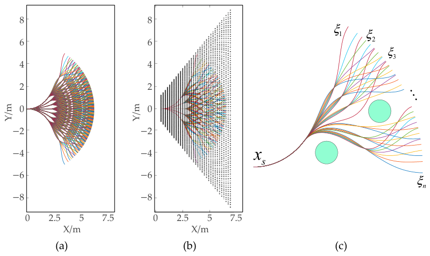
Since the probability from the starting point to the target point can be approximated by sampling on the sensor boundary F , the paths from the starting point to the boundary are sampled along seven directions. The angular range of the seven directions is from −27° to 27°, with an angular interval of 9° between adjacent directions. Paths generated along one direction are defined as one group, resulting in a total of seven groups. Each group of paths is further resampled along seven directions, and each new direction is continuously sampled along another seven directions until reaching the sensor boundary F . This yields 7   ×   7 = 49 paths per group. With seven groups in total, the overall number of paths is 343. Each path is generated under the vehicle’s kinematic constraints and is considered a feasible path from the starting point state x s to the sensor boundary F . Figure 6a shows the paths generated by sampling in seven directions and the overall path set. The states at the end of each path can be viewed as Monte Carlo samples of ξ i with i = 1 , 2 , , n .
After the seven groups of paths are generated, it is necessary to determine the occlusion relationship between the voxel points within the sensor sensing range and all paths to facilitate subsequent collision detection and eliminate paths that pass through obstacles. To accommodate the elongated structural profile of the drilling robot, the 3.2 m × 9 m area covered by the sensor is modeled, which is discretized into a voxel grid consisting of 161 × 451 voxels. For each voxel point, an offline search is performed in the set of path points to find all path points within a certain distance range, and the corresponding path indices of these path points are recorded. An index relationship table is thus established between all voxel points in the sensor coverage area and the occluded paths passing near each voxel point. Each row of the table consists of the indices of occluded paths passing around the corresponding voxel point. Figure 6b shows the voxel grid generated for the sensor coverage area, where each black dot represents a potential obstacle position.

3.3. Real-Time Optimal Path Search

As shown in Figure 6c, after the offline generation of all paths and the index table that maps voxels to occluding paths, collision detection can be performed based on the obstacle data scanned by the sensor, thereby identifying paths that are occluded by obstacles.
Define a Boolean function c ( ξ i ) to represent the collision relationship. If the path collides with an obstacle, c ( ξ i )   =   0 ; otherwise, c ( ξ i )   =   1 . That is,
c ξ i = 0 , ξ i   i s o c c l u d e d , 1 , o t h e r w i s e .
Combining this with (3), we obtain the following:
P B x s i = 1 n c ξ i p B ξ i i = 1 n c ξ i
According to Equation (5), the P B ( x s ) of all path groups is calculated online, and the path group with the highest P B ( x s ) is selected as the execution path for the robot. The selection rule is consistent with that in Reference [8]. The pseudocode of the real-time optimal path search algorithm is given in Algorithm 1. First, using the offline-generated paths, the index table, and the point cloud map perceived by the sensor, collision detection is performed to mark paths occluded by obstacles. If any traversable path exists, it is computed for each path group according to (5). The group with the highest is found, and the path generated by the first sampling step of that group is output as the robot’s execution path. Then, based on the robot’s own pose and the position and yaw angle difference to a nearby path point on the execution path, the linear and angular velocities are computed to control the robot to autonomously follow the execution path until it reaches the navigation target point. To prevent the drilling robot from backing up or pivoting in place within roadways, a path group constrained exclusively to forward locomotion is adopted. Specifically, the traversability probability within the 300° rear coverage of the robot is set to zero, and the original in-place rotation function is removed.
Algorithm 1 Optimal path search algorithm.
1Input: all path groups, index table mapping voxels to occluding paths, point cloud
perceived by the sensor, p B ( x j k ) .
2Output: an executable path or a signal that no path is found.
3Begin
4         Initialize all paths as not occluded / / 𝒪 ( n h )
5         For each point perceived by the sensor do 
          / / 𝒪 ( m n h )
6                Mark as occluded any path that collides with the obstacle according to the
                index table         / / 𝒪 ( n h )
7          end
8If not all paths are occluded then      / / 𝒪 ( 1 )
9                For each path group do      / / 𝒪 ( n h )
10                        Compute P B ( x s ) according to Equation (5)               / / 𝒪 ( n )
11               end
12                Find the group with the maximum and return the first-sampled path of
                that group   / / 𝒪 ( h )
13          end
14          else
15                Return “no path found”     / / 𝒪 ( 1 )
16          end
17end

4. Rear Robot Pose Perception Method Based on a Visual Fiducial Marker

4.1. AprilTag-Based Camera Pose Detection Method

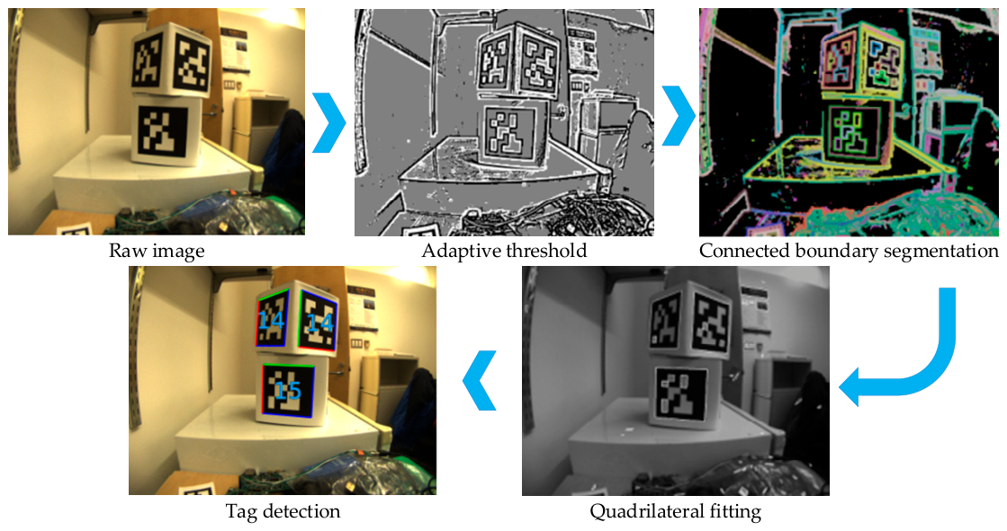
AprilTag is a visual fiducial system that provides the relative position and orientation (6-DoF) of a visual fiducial marker with respect to a camera, and it can further be used to infer the 6-DoF pose of the camera. Its main perception process is shown in Figure 7. By recognizing and decoding specific visual fiducial markers, the corresponding ID can be matched, enabling the quadrilateral boundary detection of the specific visual fiducial marker image.

4.1.1. Quadrilateral Detection

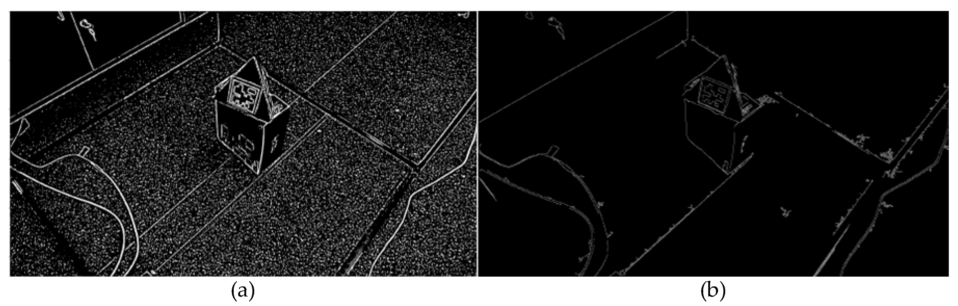
Quadrilateral detection in AprilTag is used to locate the tag region in the image. It mainly consists of three steps: adaptive thresholding, connected boundary segmentation, and quadrilateral fitting. First, we replace the original adaptive thresholding with the Canny operator for image binarization. The image is divided into blocks, and the extreme mean value of each block is computed as the threshold, enabling fast conversion from color to grayscale while effectively reducing noise, as shown in Figure 8. Subsequently, the union-find algorithm is used to separate black and white connected components and assign unique IDs. Clustering via a hash table achieves connected boundary segmentation, solving the difficulty of separating narrow-gap boundaries. Finally, the boundary points are sorted by angle, and line fitting is performed based on the Principal Component Analysis (PCA) method to identify corner points. Corner point combinations are traversed to select the valid quadrilateral with the smallest fitting error, completing tag region localization.

4.1.2. Tag Decoding

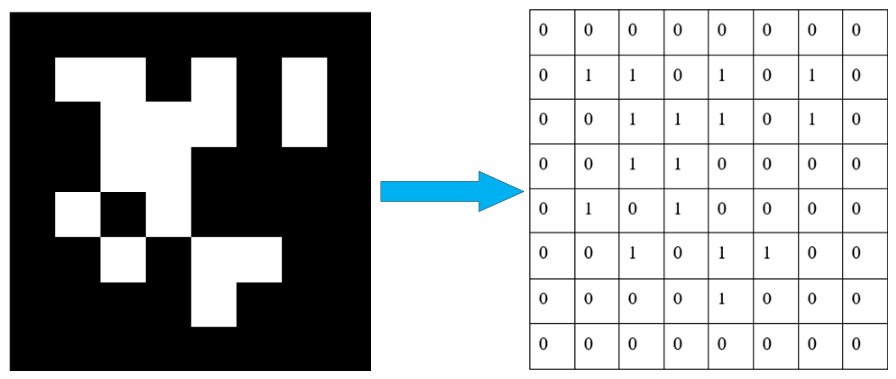
Tag decoding is used to verify the validity of the quadrilateral and to parse the tag information. The schematic diagram of tag decoding is shown in Figure 9. First, perspective correction is applied to the quadrilateral. The outer black frame and the inner encoding dot matrix are detected. Binary data are read according to 4 × 4, 5 × 5, or 6 × 6 specifications. A black-white threshold model, as shown in Equation (6), is constructed. The model parameters can be computed using least-squares regression to improve illumination robustness. Here, the bilinear form function is adopted because it models pixel intensity as a smooth function of the image coordinates (x, y) while capturing the first-order cross-illumination gradient B x y ; this allows the least-squares fit to compensate for the non-uniform lighting gradients commonly encountered in under-ground mine environments without introducing higher-degree terms that would increase fitting cost. The threshold used for decoding the tag data bits is the average of the predicted values from the black-white threshold model. Considering that the tag may have four rotational orientations (0°, 90°, 180°, and 270°), the code is rotated sequentially and matched against the code library. When the Hamming distance is less than the set threshold, the tag is considered valid, and the ID and corresponding rotation direction are output.
I ( x , y ) = A x + B x y + C y + D

4.2. Visual Label Localization Method Based on Perspective-N-Point

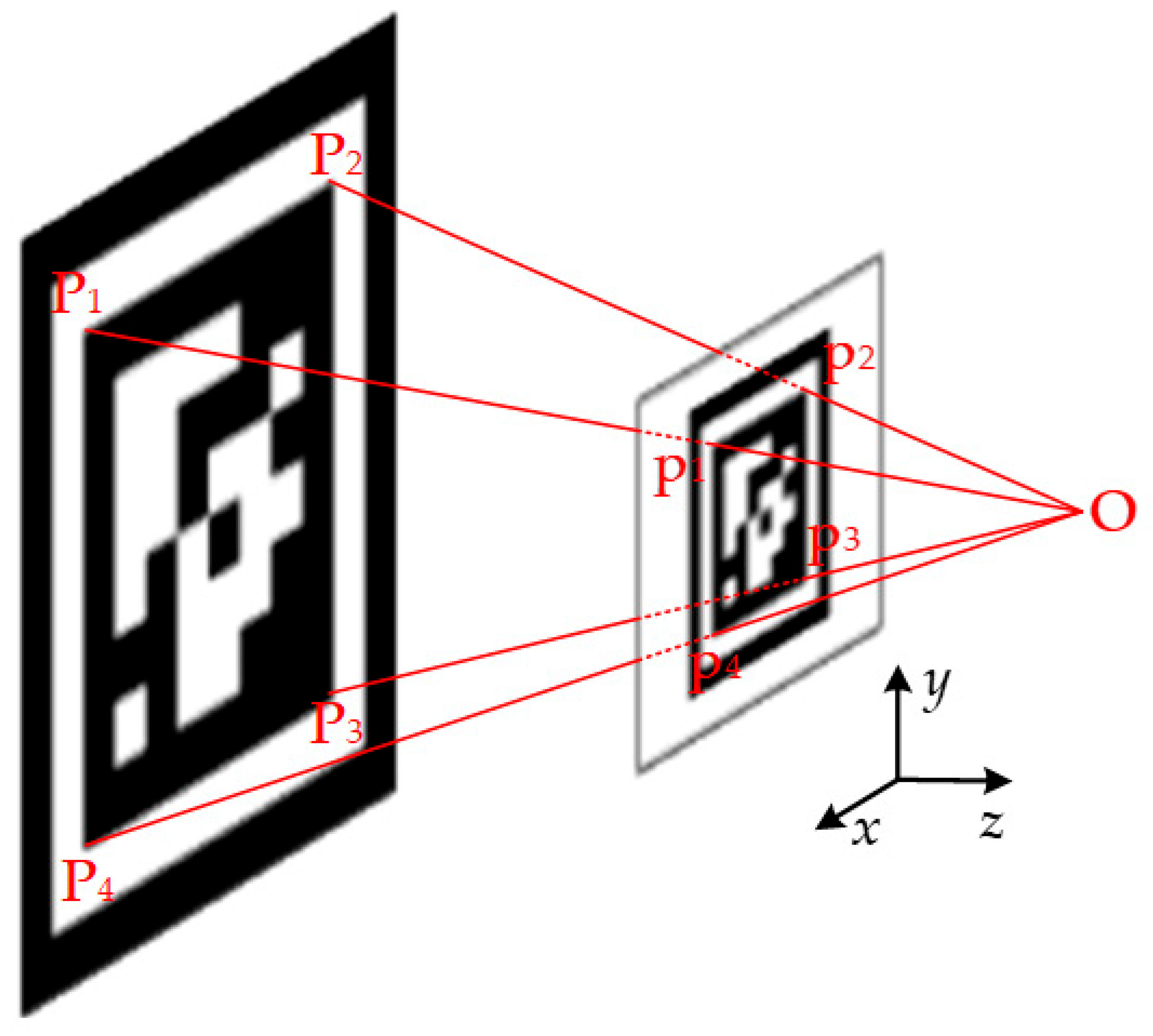
After correctly identifying the quadrilateral boundaries of the AprilTag in the image, the four corner points of the quadrilateral can be associated with their corresponding 3D world coordinate points. By constructing a Perspective-N-Point (PnP) model of the camera and the AprilTag, as shown in Figure 10, the Direct Linear Transform (DLT) is then used to compute the 6-DoF pose of the AprilTag, thereby achieving registration between the AprilTag corners and the 3D world coordinate points.
In the Figure 10, P1, P2, P3, and P4 are the four corner points in the tag coordinate system, where the origin is at the tag center, the x-axis and y-axis are parallel to the adjacent sides of the tag rectangle, and the z-axis is perpendicular to the tag plane. Their coordinate values can be calculated from the actual physical dimensions of the tag. p1, p2, p3, and p4 are the corresponding projected positions on the imaging plane. Since this paper adopts the pinhole camera model, distortion correction and camera calibration are required to obtain optimal data. For a pair of matched points, according to the camera imaging model,
s x c y c 1 = K R t 0 1 x w y w z w 1 ,
where s is the image scale factor; [ x c , y c , 1 ] T is the homogeneous coordinates of the projected point; ( x c , y c ) is the coordinates after distortion correction, computed as shown in Equation (8); ( x , y ) is the uncorrected point coordinates; ( x 0 , y 0 ) is the principal point offset; α , β , λ , δ , ε are the camera distortion parameters; K   =   [ f x , 0 , x 0 , 0 ; 0 , f y , y 0 , 0 ; 0 , 0 , 1 , 0 ] T is the camera intrinsic matrix, typically obtained through calibration; R = [ R x x , R x y , R x z ; R y x , R y y , R y z ; R z x , R z y , R z z ] T and t = [ t x , t y , t z ] T are the desired camera pose (extrinsic parameters); [ x w , y w , z w , 1 ] T is the homogeneous coordinates of the 3D point in space. In this paper, the built-in calibration tool camera_calibration in ROS is used for calibration. The camera calibration parameters are shown in Table 2.
x c = f x x c o r r e c t e d + x 0 y c = f y y c o r r e c t e d + y 0 x c o r r e c t e d = x ( 1 + α r 2 + β r 4 + λ r 6 ) + 2 δ x y + ε ( r 2 + 2 x 2 ) y c o r r e c t e d = y ( 1 + α r 2 + β r 4 + λ r 6 ) + δ ( r 2 + 2 y 2 ) + 2 ε x y
Because the tag corners are coplanar with the plane defined by the xy axes of the tag coordinate system, we have z w 0 . Then the DLT algorithm is adopted to solve the PnP problem, and the extrinsic matrix of the camera coordinates can be obtained:
x w y w 1 0 0 0 x c x w x c y w x c 0 0 0 x w y w 1 y c x w y c y w y c Φ = A Φ = 0 s . t . Φ = [ h 11 , h 12 , h 13 , h 21 , h 22 , h 23 , h 31 , h 32 , h 33 ] T
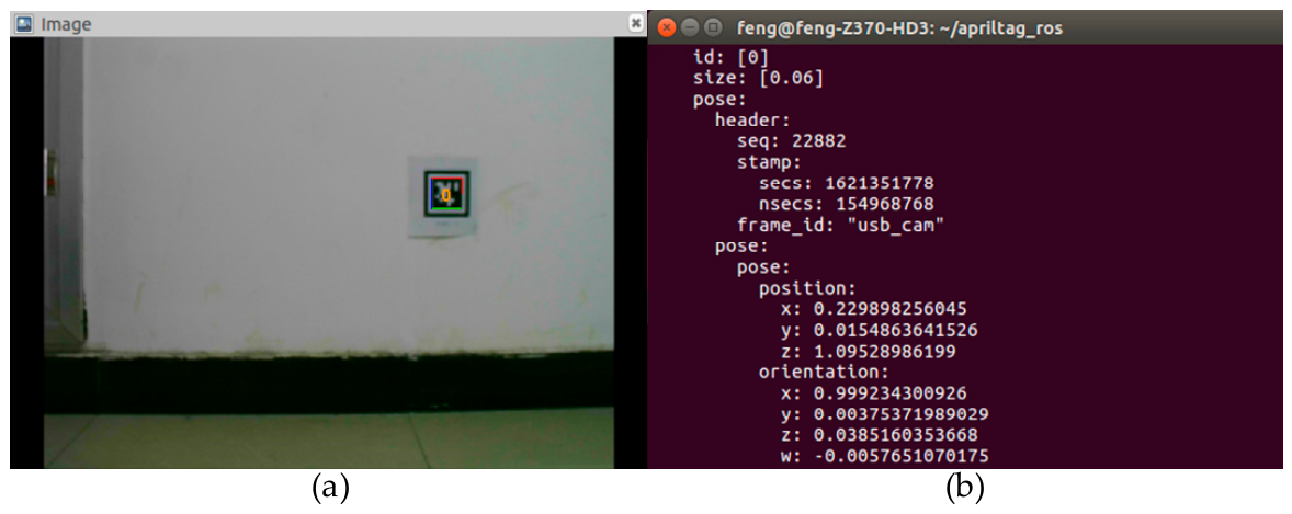
In the matrix equation, all elements of matrix A are known. Since h 33 = [ 0 , 0 , 1 ] [ t x , t y , t z ] T = t z is nonzero, to facilitate solving for the remaining eight unknowns, we can set h 33 as a constant. For convenience, let h 33 = t z = 1 . Since each feature point provides two constraint equations, matching four corner points allows us to solve the matrix Φ , thereby obtaining the first two columns of the scaled rotation matrix R and the three elements of the translation vector t . Because each column of the rotation matrix R is a unit vector, and the tag must appear in front of the camera, the scale of the matrix Φ can be determined. The rotation matrix R has orthogonality properties, so its third column can be obtained by the cross product of the first two columns. Thus, the 6-DoF pose of the tag coordinate system relative to the camera coordinate system is obtained. The localization effect is shown in Figure 11.

5. Fuzzy PID-Based Tracking Control Method for the Follower Robot

5.1. Discrete Incremental PID Method

In a typical PID controller, let r ( t ) be the desired value, y ( t ) the actual output of the controlled object, e ( t ) = r ( t ) y ( t ) the control deviation between the actual output and the desired value, and u ( t ) the controller output. The PID control law can be expressed as follows:
u ( t ) = K p [ e ( t ) + 1 T i 0 t e ( t ) d t + T d d e ( t ) d t ] ,
where K p is the proportional gain, T i the integral time constant, and T d the derivative time constant.
The tracking control error of the follower robot relative to the leader is acquired by the camera sensor and is a discrete signal. Therefore, PID must be discretized. We adopt the incremental PID method to discretize the control signal. The output is the increment of the control variable. Each output depends only on the current error and the errors of the previous two steps. If a misoperation occurs, its impact on the control variable is small, and the system stability is high. Let the sampling period be T. Then Equation (10) can be written in discrete form:
u ( k ) = k p e ( k ) + T T i i = 1 k e ( i ) + T d T [ e ( k ) e ( k 1 ) ] ,
where e ( k ) and e ( k 1 ) denote the deviations at time k and k − 1, respectively, and u ( k ) denotes the control output at time k. The output at time k − 1 can be obtained recursively as follows:
u ( k 1 ) = k p e ( k 1 ) + T T i i = 1 k 1 e ( i ) + T d T [ e ( k 1 ) e ( k 2 ) ] ,
Subtracting Equation (11) from Equation (12), the incremental PID output Δ u ( k ) is obtained as follows:
Δ u ( k ) = u ( k ) u ( k 1 ) = k p [ e ( k ) e ( k 1 ) ] + k p T T i e ( k ) + k p T d T [ e ( k ) 2 e ( k 1 ) + e ( k 2 ) ] .

5.2. Design of a Fuzzy PID-Based Tracking Controller

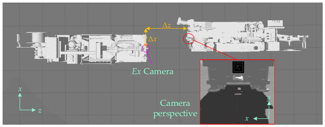
Since the drilling robot has only three controllable degrees of freedom ( x , y , θ ) when moving on the ground, only the translational error of the target along the x-axis in the two-dimensional image and the spatial distance error z are considered in the design of the visual tracking controller, while the error along the image y-axis is neglected. The schematic diagram of the tracking control and the definition of the coordinate axes for the front and rear robots of the split-type drilling robot are shown in Figure 12.
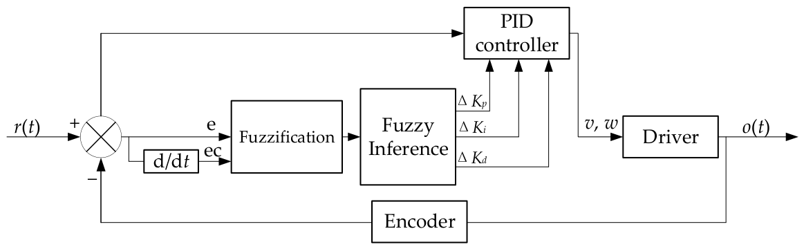
Let the coordinate of the camera of the drill pipe transportation robot relative to the two-dimensional code label at the tail of the drilling robot be [ Δ x , Δ z ] . The control errors between the camera and the AprilTag label are defined as e = [ e d , e θ ] , where e d = Δ z z 0 denotes the distance error, e θ = arctan ( Δ x / Δ z ) denotes the angle error, and z 0 is the desired tracking distance between the front and rear robots. A two-dimensional fuzzy PID controller is constructed as shown in Figure 13, in which r ( t ) represents the reference input, o ( t ) is the actual output of the controlled plant, and the control error e is taken as the input. The optimized outputs are the optimal linear velocity v and angular velocity w of the drill pipe transportation robot, thereby realizing real-time tracking of the leader by the follower for the split drilling robot.
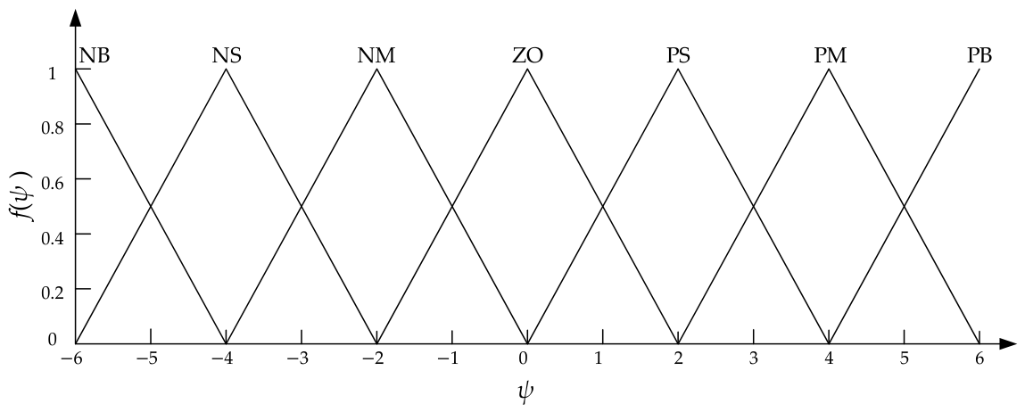
Fuzzy control is based on linguistic variables. For the error e and the error change rate ec, we use seven fuzzy linguistic variables: Negative Big (NB), Negative Medium (NM), Negative Small (NS), Zero (ZO), Positive Small (PS), Positive Medium (PM), and Positive Big (PB). The fuzzy subsets are NB ,   NS ,   NM ,   ZO ,   PS ,   PM ,   PB . Suppose the variation range of error e is [−E, E], and the variation range of error change rate ec is [−EC, EC]. The corresponding domains are both 6 ,   5 ,   4 ,   3 ,   2 ,   1 ,   0 ,   1 ,   2 ,   3 ,   4 ,   5 ,   6 . Then the input values can be fuzzified using the following quantization function:
f ( e ) = 6 e E , f ( e c ) = 6 e c E C ,
This maps all input errors e and error change rates ec onto the fuzzy domain [−6, 6]. After quantizing the input values using the above quantization function, the membership degrees of the error e or the error change rate ec can be computed. The membership values range between [0, 1]. The triangular membership function is adopted for both, which is determined by three parameters, a, b, c, with a < b < c. The function expression is given in Equation (15), where ψ donates the error e or the error change rate ec. The distribution of the membership functions corresponding to the designed fuzzy subsets is shown in Figure 14.
f ( ψ ) = ψ a b a , a < ψ b c ψ c b , b < ψ c 0 , others ,
Based on long-term accumulated field control experience and the unique motion characteristics of underground heavy-duty split drilling robots in narrow roadway environments, we summarize and formulate the fuzzy rule tables for three core output parameters of the fuzzy controller, including proportional coefficient Δ K p , integral coefficient Δ K i , and differential coefficient Δ K d . Combined with the low-speed operation, heavy-load working state, and complex vibration interference of the robot in actual coal mine scenarios, the fuzzy rules are designed following the classic control logic of coarse adjustment for large tracking deviation and fine adjustment for small deviation.

5.2.1. Fuzzy Rule Design for Δ K p

Δ K p mainly regulates the response speed of the system. Based on field control experience and the unique motion characteristics of large-aspect-ratio mine drilling robots in confined underground roadways, this study formulates the fuzzy rule table for the proportional parameter Δ K p . Table 3 shows the designed fuzzy rule table for Δ K p . Affected by its slender body structure, the robot exhibits low flexibility and weak anti-interference capability during short-range cooperative following, and it is highly sensitive to tracking position deviation. When the following error is large, a significantly increased Δ K p is adopted to rapidly improve the system response speed and quickly reduce the pose deviation between the front and rear robots. When the error is small and the error change rate is gentle, a relatively moderate proportional gain is selected to avoid excessive overshoot and attitude jitter caused by high-gain adjustment. This set of rules adapts to the low-speed and high-stability tracking requirements of large-aspect-ratio robots in narrow roadway environments.

5.2.2. Fuzzy Rule Design for Δ K i

The fuzzy rule table for the integral parameter Δ K i is formulated to meet the static error elimination demand of the heavy-duty drilling robot tracking system. Table 4 shows the designed fuzzy rule table for Δ K i . Limited by the narrow and straight roadway environment, the robot mainly performs long-distance straight-line motion, and cumulative steady-state errors are prone to occur under long-term vibration and resistance interference. In the case of large tracking errors, a small integral gain is set to prevent integral saturation and avoid system oscillation caused by rapid superposition of integral quantities. When the tracking error is maintained at a low level, an appropriate increased Δ K i is adopted to effectively eliminate residual steady-state errors and ensure long-term following accuracy. The designed rules suppress the inherent integral drift problem of traditional PID and improve the static tracking performance of the robot in stable roadway working conditions.

5.2.3. Fuzzy Rule Design for Δ K d

The fuzzy rule table for Δ K d is formulated to meet at the dynamic anti-interference demand of heavy-duty mining robots. Table 5 shows the designed fuzzy rule table for Δ K d . Complex underground disturbances, including roadway bumps and random mechanical vibration, easily cause error fluctuation. When the error changes sharply, an increased Δ K d is used to suppress dynamic mutation, absorb system oscillation, and improve anti-jitter capability. When the error changes smoothly, a low Δ K d is adopted to avoid excessive damping that weakens the system response. The designed rules match the large-inertia and vibration-sensitive characteristics of large-aspect-ratio robots, improving dynamic robustness in complex unstructured roadway environments.
After the fuzzy rule tables are established, the fuzzy subsets corresponding to Δ K p , Δ K i , and Δ K d can be inferred from the fuzzified results of the deviation e and the deviation change rate ec. Then, defuzzification is performed using the membership degrees calculated by the membership functions to obtain the quantized output values. The center-of-gravity method is used for defuzzification, with the calculation formula expressed as follows:
u 0 = ϑ u ( ϑ ) d ϑ u ( ϑ ) d ϑ ,
where u ( ϑ ) is the membership function, ϑ is the domain value of the output, and u 0 is the final quantized output value. Discretizing this yields the following:
u 0 = i = 6 6 u ( ϑ i ) ϑ i i = 6 6 u ( ϑ i ) ,
Suppose the domain of the output value is the same as that of the input value, i.e., [−6, 6], and the variation range of Δ K is [ k max , k max ] . Then the scaling factor λ between the output quantized value and the actual control quantity is as follows:
λ = k max 6 ,
Therefore, the actual output control quantity Δ K is as follows:
Δ K p , Δ K p , Δ K p = λ u 0 ,
At this point, the defuzzification process is complete. The fuzzy quantities inferred by the fuzzy rule tables are resolved into specific adjustment amounts for the PID control parameters K p , K i , and K d . The adjusted parameter values are then as follows:
K p = K p 0 + Δ K p K i = K i 0 + Δ K i K d = K d 0 + Δ K d .

6. Experiments

6.1. Simulation Experiment and Analysis

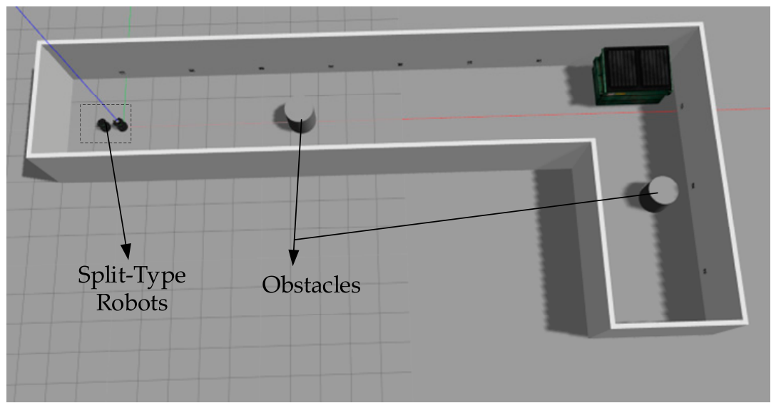
As shown in Figure 15, a simulation environment with obstacles was constructed to conduct path planning and tracking control experiments for the split-type robot. Two TurtleBot robot models were used to simulate the split-type robot. The leader performed autonomous navigation and obstacle avoidance using the path planning module, while the follower carried a camera sensor to perceive the tag information on the leader. The relative position error fed back by the tag, combined with fuzzy PID control, was used to achieve leader tracking control, thereby realizing overall navigation of the split-type robot. The parameters of the navigation module are listed in Table 6. Since the data of the positioning algorithm change in real time when the robot is moving, the set target point is a circular area with a diameter (Φ 0.2 m) rather than a single point.
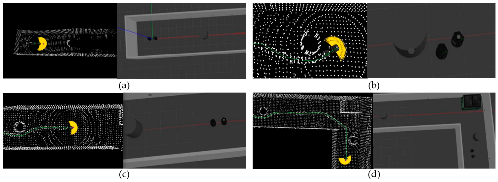
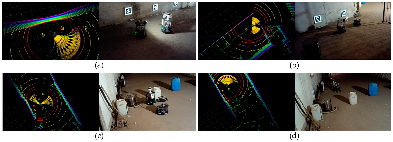
During the experiment, multiple navigation target points were set and sequentially sent to the navigation module, and the robot positions were recorded. Figure 16 shows the experimental process in the simulation environment. The left side displays the navigation information using the Rviz tool in ROS, where the white points represent the point cloud map, the yellow line represents the drivable path, and the green line represents the robot’s localization trajectory. The right side shows the corresponding scene in Gazebo. It can be observed that during navigation, the split-type robot successfully avoided obstacles and reached the final navigation position.
Table 7 lists the expected and actual values of the navigation target points. During the experiment, eight groups of desired positions were set. Each time the robot reached a set point, we waited and recorded the actual position of the robot. The error was measured as the Euclidean distance between the desired and actual positions. The maximum error during navigation is 0.166 m, and the average error is 0.156 m, the standard deviation is 0.0107 m, which can meet the practical engineering requirements.
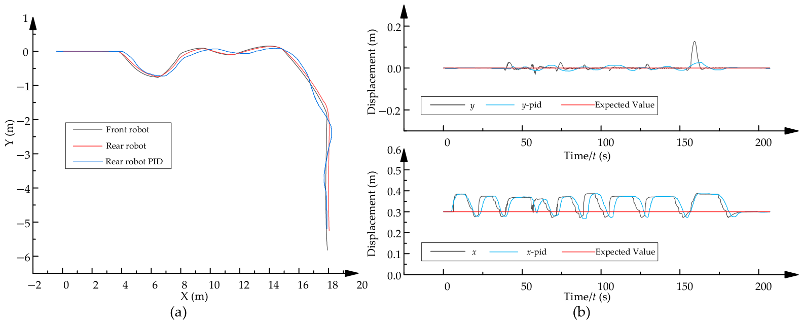
Figure 17a shows the motion trajectories of the front and rear robots of the split-type robot. It can be observed that the tracking effect of the proposed fuzzy PID-based control algorithm is good, and the trajectories of the front and rear robots are nearly coincident. The robot controlled by the classical PID exhibits noticeable left–right oscillation during the following motion. Figure 17b shows the relative position error of the rear robot with respect to the front robot during autonomous motion of the split-type robot, as fed back by the tag. The desired relative position of the rear robot with respect to the front robot is (0.3, 0), and the average tracking error obtained using the proposed algorithm is 0.05 m, while that of the traditional PID method is 0.053 m, showing little difference between the two approaches. But classical PID also suffers from obvious tracking lag in the x-direction and periodic oscillatory fluctuation in the y-direction. By contrast, the proposed fuzzy PID controller effectively suppresses trajectory oscillation and eliminates dynamic lag, delivering smoother and more stable following performance while maintaining comparable tracking accuracy. Although both controllers achieve satisfactory positioning precision, the fuzzy PID strategy possesses a faster dynamic response and gentler adjustment process, making it better suited to the large-inertia and nonlinear motion characteristics of hydraulic-driven split-type drilling robots.
The sharp error peaks appearing in Figure 17b are transient and occur during the in-situ rotation of the leader robot at the right-angle roadway corner. At this moment, the fiducial tag temporarily moves out of the effective field of view of the follower’s visual camera, causing a momentary delay in tag recognition and pose solution, which further produces a sudden increase in tracking error. After the leader finishes turning and enters straight-line motion, the follower can rapidly re-identify the tag and restore stable tracking, ensuring the continuity and reliability of the overall cooperative navigation.

6.2. Experiments in a Real Tunnel Environment

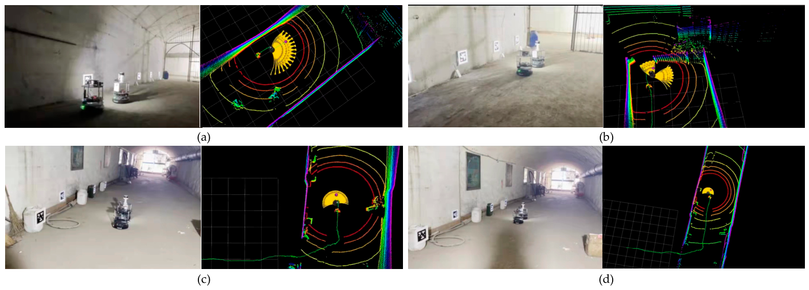
After testing in the simulation environment, autonomous navigation and tracking control experiments were conducted on the split-type robot based on localization and mapping information in a real tunnel environment to verify navigation accuracy and tracking control performance. Figure 18 shows the experimental site.

6.2.1. Experimental Process of Autonomous Walking

In the autonomous walking experiment of the split-type robot, eight desired positions relative to the odometry coordinate system were set (as shown in Table 8). Both robots are equipped with NUC 11. Its configuration includes an Intel Core i5-1145G7 processor with a 28 W TDP. It is fitted with 32 GiB DDR4 3200 MHz memory and a 500 GiB M.2 NVME 2280 solid-state drive, and it runs on the Ubuntu 18.04 operating system.
During navigation, target points were successively sent to the robot via the host computer. After reaching each target point, the robot stopped for a period while the true position was measured, and then the host computer sent the next target point until all target points had been transmitted. Figure 19 shows the navigation process. It can be observed that the autonomous walking trajectory generally coincides with the set target point trajectory. The left side shows the navigation information displayed in Rviz, where the colored points represent the point cloud map, the yellow line indicates the drivable path, and the green line shows the robot’s localization trajectory. The right side shows the corresponding real scene. Since the front and rear robots of the split-type robot belong to different control systems, only the front robot model is displayed in Rviz. The online processing time of the autonomous navigation algorithm for the robot during operation is approximately 45~65 milliseconds, and the recognition and tracking frame rate of the tracking system remains stable between 20~35 fps.
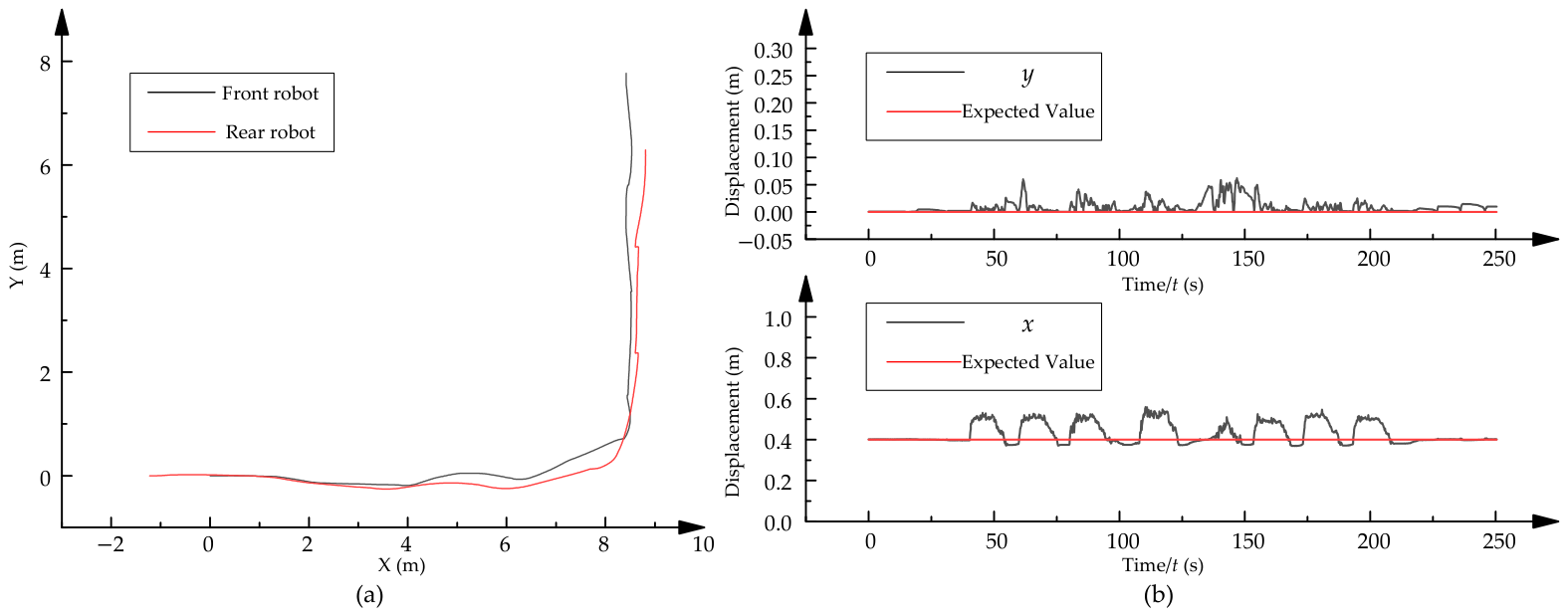
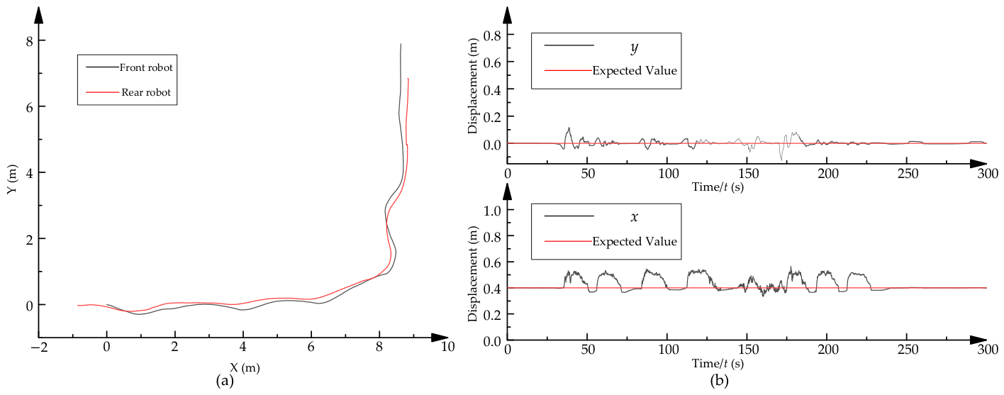
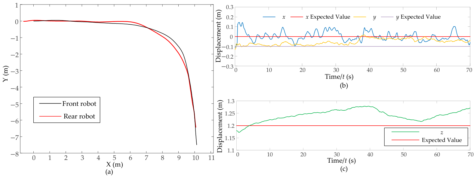
Table 8 lists the expected and measured values of the navigation target points during autonomous walking. Set the actual arrival position as a circular area with a Φ 0.2 m centered on the target point. The error is measured as the Euclidean distance between the desired and actual positions. The maximum error during navigation is 0.185 m, the average error is 0.165 m, and the standard deviation is 0.0126 m. To further verify the tracking effect of the rear robot with respect to the front robot, the trajectories of both vehicles were recorded, and the relative position error fed back by the tag was simultaneously recorded to evaluate the accuracy of the proposed fuzzy PID control algorithm. Figure 20a shows the trajectory variation curves of the front and rear robots during autonomous walking. It can be seen that the tracking effect is good, and the trajectories of the front and rear robots are nearly coincident. Figure 20b shows the relative position error of the rear robot with respect to the front robot as perceived via the tag during navigation. The desired relative position is (0.4, 0). In actual tracking, the average error in the x-direction is 0.05 m, and the average error in the y-direction is 0.01 m.

6.2.2. Obstacle Avoidance Experiment

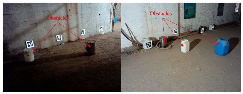
As shown in Figure 21, obstacles were added to the experimental scenario to verify the obstacle avoidance performance of the split-type robot. Figure 22 shows the obstacle avoidance process. During the experiment, multiple sets of desired positions were set. Target points were successively sent to the robot via the host computer. After reaching a target point, the robot stopped for a period, the true position was measured, and then the next target point was sent until all target points had been transmitted. The accuracy of the navigation system was evaluated using the expected and measured values. The final measurement results are shown in Table 9. Again, the error is measured as the Euclidean distance between the desired and actual positions. The maximum error during obstacle avoidance is 0.193 m, and the average error is 0.175 m, the standard deviation is 0.0152 m. The experiment demonstrates that the robot has good obstacle avoidance performance, successfully avoids obstacles, and can basically stop stably at the desired position, and its motion control accuracy meets the practical requirements. The AprilTags on the side walls are calibration points for robot positioning and were not adopted in our experiments.
Figure 23a shows the trajectory variation curves of the front and rear robots of the split-type robot during obstacle avoidance. It can be observed that when the robot avoids obstacles and stops during navigation, the trajectories of the front and rear robots deviate to some extent, but the overall trajectory overlap is high, proving that the proposed fuzzy PID-based tracking control algorithm has good tracking performance. Figure 23b shows the relative position error of the rear robot with respect to the front robot as perceived by the rear camera. The desired relative position is (0.4, 0). In actual tracking, the average tracking error in the x-direction is 0.06 m, and the average tracking error in the y-direction is 0.02 m.

6.2.3. Tracking Experiment with Large Robots

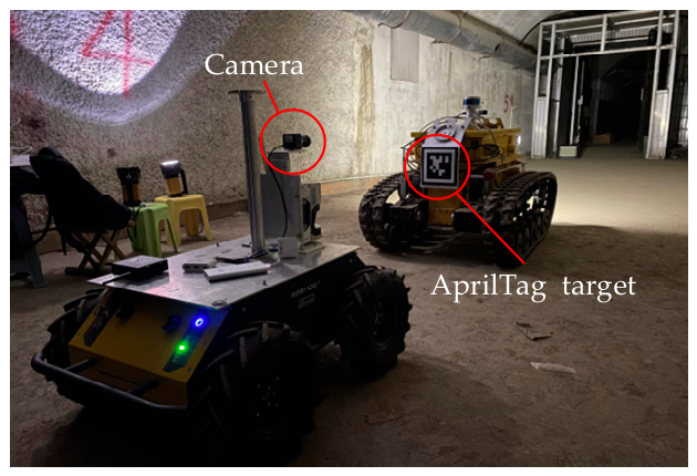
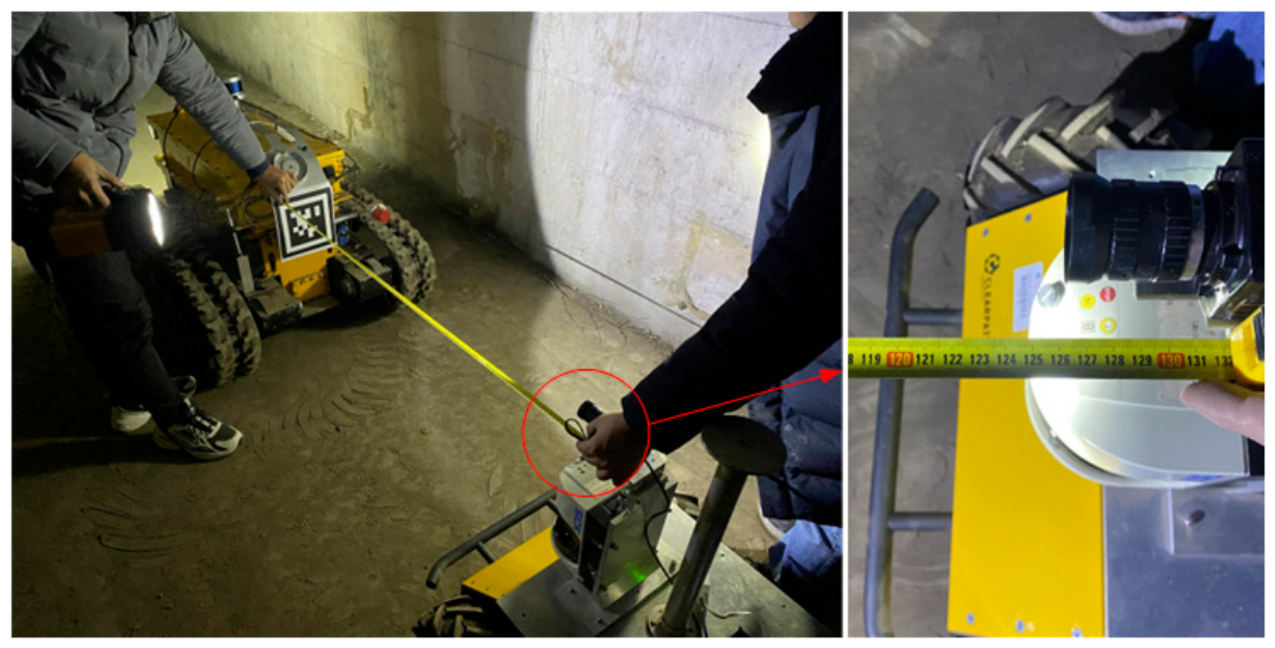
Because the drilling robot is large, the following distance between the front and rear robots is relatively long. Therefore, a larger robot was selected to further verify the performance of the tracking system. Figure 24 shows the experimental site layout. In the figure, the front robot is a coal mine rescue robot developed within our previous work [33]. A 200 mm × 200 mm AprilTag (tag36h11_0) is attached to the rear of the front robot. The rear robot is a Husky A200™ differential drive mobility platform. The hardware configuration uses the same model of industrial computer as the front robot as the computing device (same as drilling robot), and only a monocular camera is used as the visual tracking sensor to track the AprilTag target at the rear of the front robot. The tracking test parameters for the front and rear robots are set as shown in Table 10.
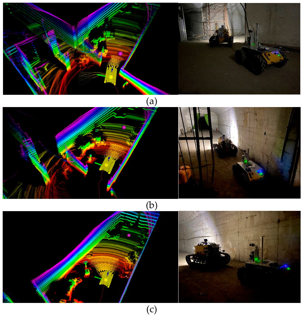
Figure 25 shows the navigation system interface during the front–rear robot tracking test and the real-time motion process of the robots in the test site. It can be seen that during the tracking process, the illumination in the tunnel environment is relatively low, and the main light source is only the searchlight on the front of the mobile test platform. Because the tracking system of the split-type robot has relatively independent control for the front and rear robots, only the navigation status of the front robot is displayed in the left navigation interface. From the figure, it can be observed that the front robot mobile test platform can turn and avoid obstacles smoothly, and the rear robot Husky A200™ can promptly track the front robot’s motion trajectory while maintaining a relatively constant tracking distance. The online processing time of the autonomous navigation algorithm for the robot during operation is approximately 25~40 milliseconds, and the recognition and tracking frame rate of the tracking system remains stable between 35~45 fps.
Figure 26 shows the trajectories of the front and rear robots of the split-type robot during tracking. The driving trajectory and positioning information of the front robot are obtained by the LiDAR odometer. The odometry data of the rear robot are collected by wheel encoders, while its positioning information is derived inversely by the visual tracking system. It can be seen that the walking paths of the two robots are almost coincident, and the final tracking distance of the rear robot remains approximately 1.2 m. The EVO toolset measured the rear robot travel distance as 14.704 m and the front robot travel distance as 15.623 m.
Figure 27 shows the actual measured distance (z-axis distance) between the front and rear robots after tracking. The measured value is 1.262 m, the algorithm detection value at the final frame is 1.277 m, and the error is 0.015 m. It can be seen that the distance control accuracy of the tracking system is extremely high. The above experiments verify the effectiveness of the target tracking algorithm and the fuzzy PID-based front–rear distance control method adopted in this paper.

6.3. Field Application Experiment of the Split-Type Drilling Robot

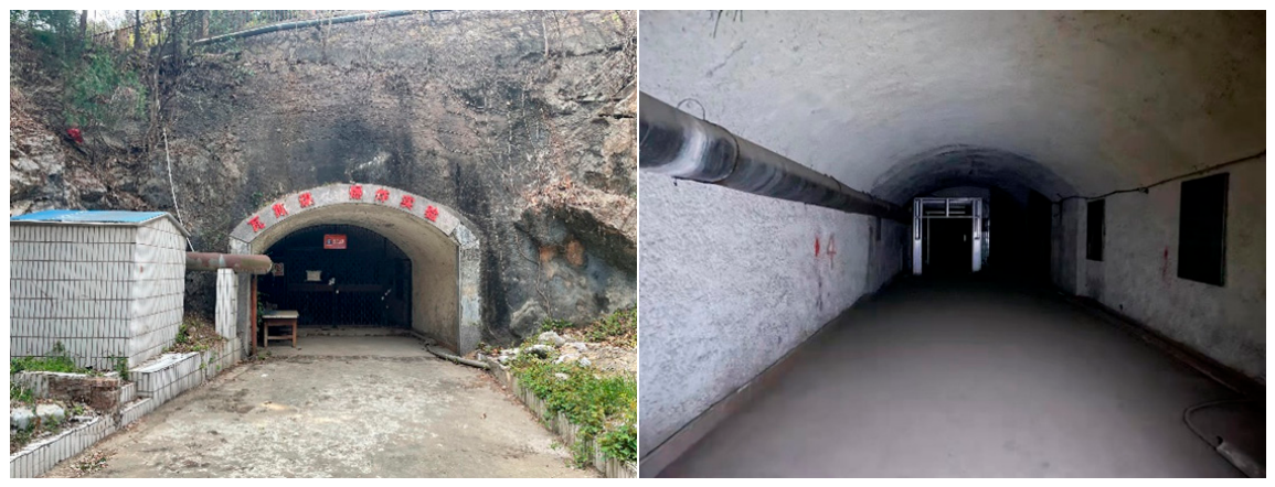
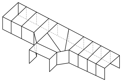
To verify the effectiveness of the proposed front–rear robot target tracking system on a coal mine drilling robot, tests were conducted in a simulated roadway at the Xi’an Research Institute of China Coal Technology & Engineering Group Corp. Figure 28 shows an isometric view of the simulated roadway test site, which is a T-shaped structure.
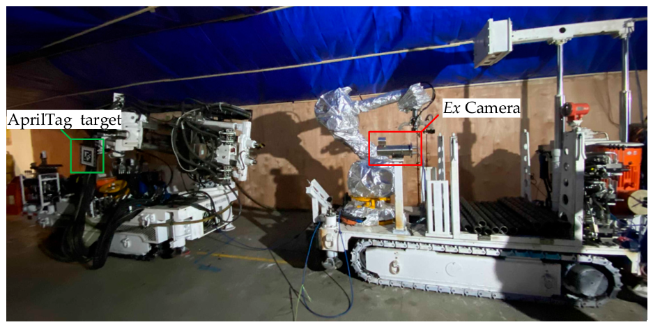
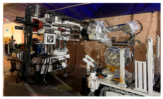
Figure 29 shows the front–rear robot tracking test site for the drilling robot. In this test, the parking coordinates of the front robot are the same as the first point in Table 5, Table 6 and Table 7 of the previous section. During actual debugging, because the bottom of the robot is occupied by hydraulic pipelines, the AprilTag could not be placed directly at the rear of the front robot. Therefore, in this test, the explosion-proof monocular camera used for positioning the rear robot manipulator (indicated by the red square in the figure) and the checkerboard plate position (indicated by the green square in the figure) on the front robot were borrowed as test equipment. The computational requirement of the visual tracking algorithm is relatively low. Therefore, the computing unit of the rear robot uses its own onboard industrial computer. Moreover, since the target is at the camera center, only a limited coordinate transformation is needed to obtain the pose relationship between the robot rotation center and the camera.
When the front robot of the drilling robot moves, the rear drill bit needs to be retracted. At this time, the rear robot cannot lock onto the target position. Therefore, the test procedure was modified as follows: after the front robot moves to the target point, the drill bit is deployed, and the rear robot starts the target tracking node and begins following. Once following is completed, the staff removes the AprilTag, and the rear robot switches to the drill pipe grabbing program, which locates the checkerboard to control the manipulator. Because the camera is not directly in front of the robot, the tracking distance must be set to ensure the safety of the protruding parts at the front of the rear robot. The tracking test parameters were set with a tracking distance threshold of 1.80 m, a tracking linear velocity of 0.15 m/s, and an angular velocity of 0.5 rad/s.
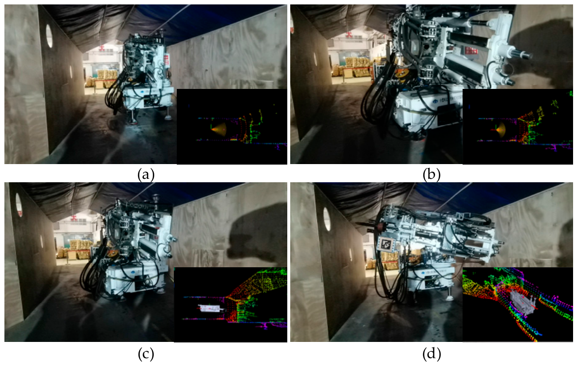
Figure 30 shows the autonomous navigation process of the lead vehicle of the drilling robot. It can be seen that after the robot moves forward to the set position, it raises the hydraulic outriggers and deploys the drill bit. After adjusting to the horizontal position, the rear robot starts tracking. The system proposed in this paper can operate in real time. The online processing time of the autonomous navigation algorithm for the robot during operation is approximately 25~40 milliseconds, and the recognition and tracking frame rate of the tracking system remains stable between 35~45 fps.
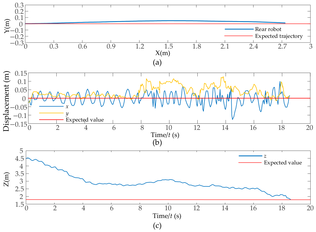
Figure 31 shows the results of the front–rear robot tracking test for the drilling robot. The figure presents the following trajectory of the rear robot, the relative error of the tracking center in the image plane, and the variation trend of the tracking distance between the front and rear robots. From Figure 31a, it can be observed that the rear robot can follow the target point and move to the set distance. Using the EVO toolkit, the rear robot travel distance was calculated. The total travel time was approximately 18.5 s, the total travel distance was 3.03 m, and the maximum deviation in the y-direction was 0.051 m. The rear robot was able to travel along an essentially straight-line trajectory. Figure 31b shows the variation of the center position deviation of the target tracked by the rear robot. The image plane takes the image center (0, 0) as the desired position. From the test results, during the gradual approach, the y-axis deviation shows an increasing trend, but the variation in the y-direction does not significantly affect the actual walking control. The x-axis deviation exhibits a sine-wave-like shape, which is caused by the robot adjusting the speeds of the left and right tracks in response to changes in the lateral position of the target. The maximum error in the x-direction is 0.10 m, and the average error is −0.002 m. Figure 31c shows the variation trend of the following distance. The rear robot of the drilling robot gradually moves from an initial position of about 4.5 m to a position about 1.8 m from the front robot and then stops. Because the lighting conditions were good, the distances at the initial and final states were measured accurately. However, some distance misjudgments occurred during the middle period due to changes in the light source. Nevertheless, the overall tracking effect was good and met the application requirements.
Figure 32 shows a schematic diagram of the completion of front–rear robot tracking for the drilling robot. The figure shows the position of the rear robot when tracking is completed while the front robot is parked at the target point. Because the front and rear robots are independent of each other, the hydraulic support has already been raised after the front robot completes navigation. Thanks to the good lighting conditions, the AprilTag target was almost entirely clearly visible throughout the tracking process, and the rear robot was able to quickly track to near the set distance range. This test verifies the effectiveness of the proposed front–rear robot visual tracking system in the practical application of the drilling robot. This test also demonstrates that using relatively independent autonomous navigation systems for the front and rear robots enables flexible configuration according to the working site conditions, offering significant advantages in the modularization of drilling robots.

7. Conclusions

This paper addressed the autonomous navigation and communication-free visual tracking problem for split-type drilling robots operating in confined underground environments. We proposed a leader–follower architecture in which the leader performs autonomous path planning using pre-computed offline trajectories and 3D LiDAR perception, while the follower estimates its relative pose via AprilTag detection and executes tracking using a fuzzy PID controller. The offline path set generation with Monte Carlo-based probabilistic evaluation enables efficient real-time navigation, and the fuzzy PID controller provides smooth and accurate tracking under dynamic conditions. Extensive experiments in simulation, a simulated tunnel, and a real coal mine roadway demonstrated that the system achieves reliable autonomous navigation, effective obstacle avoidance, and precise leader–follower distance control. The proposed method eliminates the need for inter-vehicle communication, reduces system complexity, and enhances robustness in GPS-denied, visually degraded environments. The split tracking control scheme prevents operators from moving between robots, effectively improving on-site safety. Simulation experiment results show that the tracking error of the fuzzy PID algorithm is not significantly different from that of the traditional PID algorithm, but the fuzzy PID controller achieves a smoother, less oscillatory response, making it better suited to the large-inertia characteristics of hydraulic-driven split-type drilling robots. The fuzzy PID controller achieves comparable tracking accuracy with a smoother, less oscillatory response, making it better suited to the large-inertia characteristics of hydraulic-driven split-type drilling robots. These results confirm the feasibility of deploying the system in practical coal mine drilling operations and provide a foundation for future extensions to multi-robot coordination in similar applications.
In future work, we will carry out the multi-dimensional optimization of the robot cooperative tracking system for complex underground mining environments. First, a multi-tag fusion positioning method will be introduced to optimize the visual localization architecture, where multiple fiducial tags will be arranged on the leader robot for redundant pose solving. It could effectively compensate for the defects of single-tag tracking, avoid intermittent tracking anomalies, and improve the anti-interference performance and tracking stability in complex underground roadways. Second, targeted image processing strategies for dust removal, defogging, and low-light enhancement will be developed to address image degradation caused by dust contamination and extreme low-light conditions in underground roadways, further improving the environmental robustness and engineering practicability of the system. On this basis, we will integrate multi-sensor perception and end-to-end learning methods to enhance the tracking accuracy under high-speed motion and strong disturbance. Finally, the optimized framework will be generalized to more split-type robots for confined-space operations, expanding the engineering application boundary of the system.

Author Contributions

Conceptualization, S.Y. and Y.D.; methodology, S.Y.; software, Y.D.; validation, S.Y. and Y.D.; formal analysis, M.L.; investigation, S.Y. and C.T.; resources, S.Y.; data curation, M.L.; writing—original draft preparation, S.Y.; writing—review and editing, C.T.; visualization, M.L.; supervision, C.T.; project administration, C.T.; funding acquisition, S.Y. All authors have read and agreed to the published version of the manuscript.

Funding

This research was funded by the National Natural Science Foundation of China (grant number: 52504178, 52304183), the National Key Research and Development Program of China (grant number: 2024YFB2908801), and in part by the Project Funds of the Priority Academic Program Development (PAPD) of Jiangsu Higher Education Institutions.

Institutional Review Board Statement

Not applicable.

Informed Consent Statement

Not applicable.

Data Availability Statement

The datasets presented in this article are not readily available because of time and experimental site environment limitations. Requests to access the datasets should be directed to the correspondence author.

Conflicts of Interest

The authors declare no conflicts of interest.

Appendix A

Table A1 in Appendix A compares the various performances, advantages, and disadvantages of five visual fiducial markers. Bold contents in the table indicate superior performance compared with other methods.
Table A1. Performance comparison of mainstream visual fiducial markers.
Marker TypeAprilTagArUcoChArUcoARToolKitQR Code
Error
Correction
Capability
Strong (tag36h11/tag25h9)Limited error
tolerance
No dedicated robust error-correcting codingProne to feature confusionNot designed for pose positioning
Positioning
Accuracy
Sub-millimeter
accuracy at close range, 6DOF pose
Moderate accuracy; corners vulnerable to noiseHigh accuracy via chessboard sub-pixel detection, relying on complete grid pointsLow accuracy and unstable
corner extraction
Low accuracy with only four corners and no sub-pixel optimization
Running
Speed
Moderate (15–20 fps on embedded devices)Fastest (30+ fps with OpenCV optimization)Relatively slow due to dual computationModerateHigh
Resistance to Light/ShadowHigh robustnessProne to detection loss under varying lightHighly dependent on image contrastWeak resistance to light changesPoor resistance to light variation and blurring
Occlusion
Resistance
Tolerates partial occlusion; single tag works independentlyDetection fails
easily under partial occlusion
Good tolerance using remaining corners, but requires large visible areaPoor occlusion toleranceModerate
occlusion
tolerance
Effective
Detection
Range
Long range, up to 50 times the tag sizeShort range; invalid when blurred at a distanceModerate range; grid points blur at long distancesOnly effective at close rangeOnly effective
at close range
Rotation
Robustness
High adaptability
to planar and
spatial rotation
Poor performance at large angles and long distancesAverage performance; large-angle distortion affects corner extractionPoor performanceAverage
performance
Ecosystem & ApplicationNatively supported by ROSBuilt into OpenCV; lightweight and easy to implementSupported by OpenCV; mainly for camera
calibration
Classic early AR solution, now gradually phased outUniversal information carrier, widely used on mobile devices
DisadvantagesSlightly slower than ArUcoLow accuracy and robustness;
unstable in poor lighting scenarios
Large size for
deployment, no independent ID
High false
detection rate and poor overall robustness;
Not suitable for high-precision
robot tracking

References

  1. Zhao, J.; Han, Z.; Liu, G. Development of a serpentine omnitread robot for searching in explosive gas atmospheres. Ind. Robot Int. J. 2011, 38, 469–475. [Google Scholar] [CrossRef] [Scilit]
  2. Zheng, Z.; Zhang, W.; Fu, X.; Hazken, S.; Hu, X.; Chen, H.; Luo, J.; Ding, N. Ccrobot-iv: An obstacle-free split-type quad-ducted propeller-driven bridge stay cable-climbing robot. IEEE Robot. Autom. Lett. 2021, 7, 11751–11758. [Google Scholar] [CrossRef] [Scilit]
  3. Han, M.; Zhou, J.; Chen, X.; Li, L. Analysis of in-pipe inspection robot structure design. In Proceedings of the 2016 2nd Workshop on Advanced Research and Technology in Industry Applications (WARTIA-16); Atlantis Press: Paris, France, 2016; pp. 987–991. [Google Scholar]
  4. Zhang, S.; Lin, W.; Chen, W.; Chen, C. The application of a novel split-type robotic system, Carina Platform, for esophageal surgery. J. Clin. Oncol. 2025, 43, e16145. [Google Scholar] [CrossRef] [Scilit]
  5. Zhou, B.; Xu, H.; Shen, S. Racer: Rapid collaborative exploration with a decentralized multi-uav system. IEEE Trans. Robot. 2023, 39, 1816–1835. [Google Scholar] [CrossRef] [Scilit]
  6. Yan, J.; Lin, X.; Ren, Z.; Zhao, S.; Yu, J.; Cao, C.; Yin, P.; Zhang, J.; Scherer, S. MUI-TARE: Cooperative multi-agent exploration with unknown initial position. IEEE Robot. Autom. Lett. 2023, 8, 4299–4306. [Google Scholar] [CrossRef]
  7. Wang, Z.; Zhou, X.; Xu, C.; Gao, F. Geometrically constrained trajectory optimization for multicopters. IEEE Trans. Robot. 2022, 38, 3259–3278. [Google Scholar] [CrossRef] [Scilit]
  8. Zhang, J.; Hu, C.; Chadha, R.G.; Singh, S. Falco: Fast likelihood-based collision avoidance with extension to human-guided navigation. J. Field Robot. 2020, 37, 1300–1313. [Google Scholar] [CrossRef] [Scilit]
  9. Tordesillas, J.; How, J.P. MADER: Trajectory planner in multiagent and dynamic environments. IEEE Trans. Robot. 2021, 38, 463–476. [Google Scholar] [CrossRef] [Scilit]
  10. Zhou, X.; Wen, X.; Wang, Z.; Gao, Y.; Li, H.; Wang, Q.; Yang, T.; Lu, H.; Cao, Y.; Xu, C. Swarm of micro flying robots in the wild. Sci. Robot. 2022, 7, eabm5954. [Google Scholar] [CrossRef] [Scilit]
  11. Olson, E. AprilTag: A robust and flexible visual fiducial system. In Proceedings of the 2011 IEEE International Conference on Robotics and Automation; IEEE: Piscataway, NJ, USA, 2011; pp. 3400–3407. [Google Scholar]
  12. Wang, J.; Olson, E. AprilTag 2: Efficient and robust fiducial detection. In Proceedings of the 2016 IEEE/RSJ International Conference on Intelligent Robots and Systems (IROS); IEEE: Piscataway, NJ, USA, 2016; pp. 4193–4198. [Google Scholar]
  13. Yu, C.; Cai, J.; Chen, Q. Multi-resolution visual fiducial and assistant navigation system for unmanned aerial vehicle landing. Aerosp. Sci. Technol. 2017, 67, 249–256. [Google Scholar] [CrossRef] [Scilit]
  14. Romero-Ramirez, F.J.; Muñoz-Salinas, R.; Medina-Carnicer, R. Speeded up detection of squared fiducial markers. Image Vis. Comput. 2018, 76, 38–47. [Google Scholar] [CrossRef] [Scilit]
  15. Calvet, L.; Gurdjos, P.; Griwodz, C.; Gasparini, S. Detection and accurate localization of circular fiducials under highly challenging conditions. In Proceedings of the IEEE Conference on Computer Vision and Pattern Recognition; IEEE: Piscataway, NJ, USA, 2016; pp. 562–570. [Google Scholar]
  16. Brunner, C.; Peynot, T. Perception quality evaluation with visual and infrared cameras in challenging environmental conditions. In Proceedings of the Experimental Robotics: The 12th International Symposium on Experimental Robotics; Springer: Berlin/Heidelberg, Germany, 2014; pp. 711–725. [Google Scholar]
  17. Yuanwei, C.; Zaman, M.H.M.; Ibrahim, M.F. A review on six degrees of freedom (6D) pose estimation for robotic applications. IEEE Access 2024, 12, 161002–161017. [Google Scholar] [CrossRef] [Scilit]
  18. Wang, J.; Wu, P.; Zhang, X.; Xu, R.; Wang, T. Six-Degree-of-Freedom Pose Estimation Method for Multi-Source Feature Points Based on Fully Convolutional Neural Network. J. Intell. Robot. Syst. 2024, 110, 131. [Google Scholar] [CrossRef] [Scilit]
  19. Castellanos-Cárdenas, D.; Posada, N.L.; Orozco-Duque, A.; Sepúlveda-Cano, L.M.; Castrillón, F.; Camacho, O.E.; Vásquez, R.E. A review on data-driven model-free sliding mode control. Algorithms 2024, 17, 543. [Google Scholar] [CrossRef] [Scilit]
  20. Howard, T.; Pivtoraiko, M.; Knepper, R.A.; Kelly, A. Model-predictive motion planning: Several key developments for autonomous mobile robots. IEEE Robot. Autom. Mag. 2014, 21, 64–73. [Google Scholar] [CrossRef] [Scilit]
  21. Ismael, O.Y.; Almaged, M.; Abdulla, A.I. Nonlinear model predictive control-based collision avoidance for mobile robot. J. Robot. Control (JRC) 2024, 5, 142–151. [Google Scholar] [CrossRef] [Scilit]
  22. Meng, D.; Chu, H.; Tian, M.; Gao, B.; Chen, H. Real-time high-precision nonlinear tracking control of autonomous vehicles using fast iterative model predictive control. IEEE Trans. Intell. Veh. 2024, 9, 3644–3657. [Google Scholar] [CrossRef] [Scilit]
  23. Li, L.; Miao, Y.; Qureshi, A.H.; Yip, M.C. MPC-MPNet: Model-predictive motion planning networks for fast, near-optimal planning under kinodynamic constraints. IEEE Robot. Autom. Lett. 2021, 6, 4496–4503. [Google Scholar] [CrossRef] [Scilit]
  24. Askari, I.; Vaziri, A.; Tu, X.; Zeng, S.; Fang, H. Model predictive inferential control of neural state-space models for autonomous vehicle motion planning. IEEE Trans. Robot. 2025, 41, 3202–3222. [Google Scholar] [CrossRef] [Scilit]
  25. Wahyuni, S.; Fuad, M.; Hilda, A.D.D.; Umam, F.; Latif, M. Enhancing Mobile Robot Stability and Roaming Capability Using Fuzzy-PID Control Method. In Proceedings of the 2023 IEEE 9th Information Technology International Seminar (ITIS); IEEE: Piscataway, NJ, USA, 2023; pp. 1–6. [Google Scholar]
  26. Tolossa, T.D.; Gunasekaran, M.; Halder, K.; Verma, H.K.; Parswal, S.S.; Jorwal, N.; Joseph, F.O.M.; Hote, Y.V. Trajectory tracking control of a mobile robot using fuzzy logic controller with optimal parameters. Robotica 2024, 42, 2801–2824. [Google Scholar] [CrossRef] [Scilit]
  27. Hailu, G.L.; Yatayew, T.T. Intelligent trajectory tracking in autonomous plantation robots using PSO-tuned nonlinear fuzzy PID, fuzzy PID, and conventional PID controllers. Sci. Rep. 2025, 15, 45357. [Google Scholar] [CrossRef] [Scilit] [PubMed]
  28. Pérez-Juárez, J.G.; García-Martínez, J.R.; Medina Santiago, A.; Cruz-Miguel, E.E.; Olmedo-García, L.F.; Barra-Vázquez, O.A.; Rojas-Hernández, M.A. Kinematic fuzzy logic-based controller for trajectory tracking of wheeled mobile robots in virtual environments. Symmetry 2025, 17, 301. [Google Scholar] [CrossRef] [Scilit]
  29. Benaicha, I.; Nechadi, E.; Boutalbi, O.; Essounbouli, N. An Improved Fuzzy Logic Controller for Mobile Robots Navigation in Unknown Environments. J. Field Robot. 2026, 43, 257–278. [Google Scholar] [CrossRef] [Scilit]
  30. He, H.; Liu, Q.; Shentu, S.; Gong, Z. Trajectory tacking controller design for wheeled robots in multi-robot cooperative transport. J. Mech. Eng. 2024, 60, 145–155. [Google Scholar] [CrossRef] [Scilit]
  31. Cosenza, C.; Malfi, P.; Melluso, F.; Nicolella, A.; Niola, V.; Savino, S.; Spirto, M.; Tordela, C. A Virtual Sensor for Wheel Angular Speed Estimation: Application on a Differential Drive Wheeled Robot. J. Intell. Robot. Syst. 2025, 111, 117. [Google Scholar] [CrossRef] [Scilit]
  32. You, S.; Li, M.; Wu, B.; Wang, J.; Tang, C. Digital Twin of Coal Mine Rescue Robot—Research on Intelligence and Visualization. Sensors 2026, 26, 2840. [Google Scholar] [CrossRef] [Scilit] [PubMed]
  33. Li, Y.; Li, M.; Zhu, H.; Hu, E.; Tang, C.; Li, P.; You, S. Development and applications of rescue robots for explosion accidents in coal mines. J. Field Robot. 2020, 37, 466–489. [Google Scholar] [CrossRef] [Scilit]
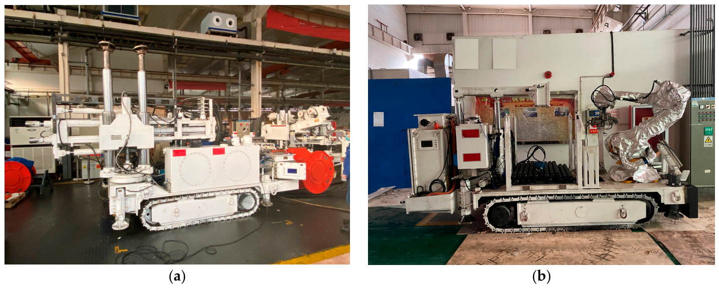
Figure 1. Physical prototype of the drilling robot. (a) Front robot: ZDY4000LK Drilling Robot; (b) Rear robot: ZY30LK Drill Pipe Transport Robot.
Applsci 16 05929 g001
Figure 2. Hardware–software framework of autonomous navigation and visual tracking system for coal mine drilling robots.
Applsci 16 05929 g002
Figure 3. Diagram of front–rear robot tracking for the coal mine drilling robot. Ex: Explosion-proof Grade Certification for Coal Mining Equipment in China. MA: Mine Safety Certification for Coal Mining Products in China.
Applsci 16 05929 g003
Figure 4. Navigation system interface design. The title bar of the page displays the institution name. The tabs in the upper-left corner of the page are Start and Display respectively. The two buttons at the bottom right of the right figure are Start and Stop. In the right figure, the white mouse cursor is used to drag the view of the navigation interface. The purple lines in the navigation interface represent passable paths, the thin green line behind the robot indicate its travel trajectory, the red circles stand for ground-scanned point clouds, and the rectangles enclosed by light green point clouds simulate the walls of the roadway.
Applsci 16 05929 g004
Figure 5. Schematic diagram of route planning.
Applsci 16 05929 g005
Figure 6. Generated schematic diagram of the offline path set and collision detection. (a) Schematic diagram of path group generation. (b) Schematic diagram of sensor perception area modeling. (c) Schematic diagram of collision detection.
Applsci 16 05929 g006
Figure 7. AprilTag label recognition flow chart.
Applsci 16 05929 g007
Figure 8. Comparison results of two image binarization processing algorithms. (a) Adaptive threshold; (b) binarization result using the Canny operator.
Applsci 16 05929 g008
Figure 9. Schematic diagram of tag decoding.
Applsci 16 05929 g009
Figure 10. Schematic diagram of the PnP model.
Applsci 16 05929 g010
Figure 11. Positioning effect diagram. (a) Camera image; (b) positioning data.
Applsci 16 05929 g011
Figure 12. Schematic diagram of front and rear robot tracking control.
Applsci 16 05929 g012
Figure 13. Principle block diagram of the fuzzy PID controller.
Applsci 16 05929 g013
Figure 14. Triangular membership function distribution diagram.
Applsci 16 05929 g014
Figure 15. Navigation simulation environment. The red, green and blue rays in the figure represent the x, y and z axes of the world coordinate system.
Applsci 16 05929 g015
Figure 16. Experimental process in the simulation scenario. (a) Start navigation. (b) Obstacle avoidance. (c) Straight walking. (d) Reach the destination. In the figure, yellow lines represent passable paths, green lines denote traveled trajectories, white points are laser point clouds, and purple dots stand for navigation target points. The red, green and blue rays in the figure represent the x, y and z axes of the world coordinate system.
Applsci 16 05929 g016
Figure 17. Experimental results of split-type robot navigation and tracking. (a) Front and rear trajectories of the split-type robot. (b) Relative position error variation curve.
Applsci 16 05929 g017
Figure 18. Experimental environment. The red text in the figure: Gas and Coal Dust Explosion Laboratory.
Applsci 16 05929 g018
Figure 19. Experimental process of autonomous walking. (a) Start navigation. (b) Prepare to turn. (c) Turn completed. (d) Reach the destination. In the figure, the green line behind the robot represent its travel trajectory, yellow lines in front of the robot represent passable paths, purple dots stand for navigation target points. The colored lines represent the laser point cloud, with colors ranging from red to purple indicating the height of the point cloud.
Applsci 16 05929 g019
Figure 20. Quantitative analysis results of autonomous walking control for front and rear robots. (a) Trajectory variation curves of the front and rear robots during autonomous walking. (b) Relative position error of the front and rear robots during autonomous walking.
Applsci 16 05929 g020
Figure 21. Obstacle avoidance experiment environment.
Applsci 16 05929 g021
Figure 22. Obstacle avoidance experiment process. (a) Avoid obstacles. (b) Traverse the door. (c) Traverse narrow areas. (d) Reach the destination. In the figure, the green line behind the robot represent its travel trajectory, yellow lines in front of the robot represent passable paths,, purple dots stand for navigation target points. The colored lines represent the laser point cloud, with colors ranging from red to purple indicating the height of the point cloud.
Applsci 16 05929 g022
Figure 23. Quantitative analysis results of obstacle avoidance experiment control for front and rear robots. (a) Trajectory curves of the front and rear robots during obstacle avoidance. (b) Relative position error of the front and rear robots during obstacle avoidance.
Applsci 16 05929 g023
Figure 24. Front and rear robots’ tracking experiment site.
Applsci 16 05929 g024
Figure 25. Front and rear robot tracking test site and navigation interface display. (a) Before the front robot turns. (b) After the front robot turns. (c) Turn completed. In the figure, the red line behind the robot represent its travel trajectory, yellow lines in front of the robot represent passable paths, purple dots stand for navigation target points, and the dark yellow geometric body is the robot model. The colored lines represent the laser point cloud, with colors ranging from red to purple indicating the height of the point cloud.
Applsci 16 05929 g025
Figure 26. Quantitative analysis results of navigation and tracking control for the front and rear robots of large-scale robots. (a) Trajectory diagram of front and rear car tracking. (b) Relative error of tracking center in the image plane. (c) Variation in front–rear robot tracking distance.
Applsci 16 05929 g026
Figure 27. Actual tracking distance between front and rear robots.
Applsci 16 05929 g027
Figure 28. Isometric side view of the simulated roadway test site.
Applsci 16 05929 g028
Figure 29. Drilling robot front and rear robot tracking test site.
Applsci 16 05929 g029
Figure 30. Autonomous navigation process of the drilling robot (front robot). The navigation interface is shown in the lower right corner. (a) Start navigation, (b) during autonomous walking, (c) reaching the drilling position, and (d) deploying the drill bit. In the figure, yellow lines represent passable paths, red line denote traveled trajectory, purple dots stand for navigation target points, and the gray geometric body is the robot model. The colored dots represent the laser point cloud, with colors ranging from red to purple indicating the height of the point cloud.
Applsci 16 05929 g030
Figure 31. Drilling robot front and rear robot tracking test results. (a) Rear robot following trajectory. (b) Relative error of tracking center in the image plane. (c) Variation of front–rear robot tracking distance.
Applsci 16 05929 g031
Figure 32. Drilling robot front and rear robot tracking completed.
Applsci 16 05929 g032
Table 1. Parameters of the drilling robot and drill pipe transport robot.
PropertyZDY4000LK Drilling RobotZY30LK Drill Pipe Transport Robot
Dimensions (L × W × H)5500 mm × 1250 mm × 2280 mm5050 mm × 1150 mm × 1850 mm
Mass8300 kg6500 kg (unloaded)
Chassis typeTrackedTracked
Travel speed0.9 km/h0.9 km/h
Drive modeHydraulicHydraulic
Motion modeDifferential driveDifferential drive
Gradeability15°15°
Supply voltage1140 V1140 V
Table 2. Calibration matrix.
ParameterMatrix
Intrinsic matrix 632.36696 0 325.08902 0 632.55799 163.89233 0 0 1
Distortion coefficient matrix[−0.117210  0.110626  −0.001189  −0.002173  0]
Rectification matrix 1 0 0 0 1 0 0 0 1
Projection matrix 617.49854 0 324.1099 0 0 620.70972 161.87488 0 0 0 1 0
Table 3. Fuzzy rule table for Δ K p .
ecNBNMNSZOPSPMPB
e
NBPBPBPMPMPSZOZO
NMPBPBPMPSPSZONS
NSPMPMPMPSZONSNS
ZOPMPMPSZONSNMNM
PSPSPSZONSNSNMNM
PMPSZONSNMNMNMNB
PBZOZONMNMNMNBNB
Table 4. Fuzzy rule table for Δ K i .
ecNBNMNSZOPSPMPB
e
NBNBNBNMNMNSZOZO
NMNBNBNMNSNSZOZO
NSNBNMNSNSZOPSPS
ZONMNMNSZOPSPMPM
PSNMNSZOPSPSPMPB
PMZOZOPSPSPMPBPB
PBZOZOPSPMPMPBPB
Table 5. Fuzzy rule table for Δ K d .
ecNBNMNSZOPSPMPB
e
NBPSNSNBNBNBNMPS
NMPSNSNBNMNMNSZO
NSZONSNMNMNSNSZO
ZOZONSNSNSNSNSZO
PSZOZOZOZOZOZOZO
PMPBNSPSPSPSPSPB
PBPBPMPMPMPSPSPB
Table 6. Navigation parameters for simulation experiment.
ParameterFront Robot Planning SpeedRear Robot Tracking SpeedNavigation
Interval
Arrival
Threshold
Desired Tracking DistanceConfidence
Threshold
Value0.2 m/s0.25 m/s8 sΦ 0.2 m0.3 m0.6
Table 7. Expected and actual values of navigation target points.
No.True Value/mActual Value/mError/mStd Dev/m
1(2, 0, 0)(1.84, −0.01, 0)0.160-
2(4, 0, 0)(3.85, 0, 0)0.150-
3(8, 0, 0)(7.89, −0.12, 0)0.163-
4(10, 0, 0)(9.84, 0.02, 0)0.161-
5(12, 0, 0)(11.87, −0.03, 0)0.133-
6(15, 0, 0)(14.85, 0.04, 0)0.155-
7(18, −2, 0)(17.88, −1.89, 0)0.163-
8(18, −6, 0)(17.93, −5.85, 0)0.166-
Average error 0.1560.0107
Table 8. Expected and measured values during autonomous walking.
No.True Value/mActual Value/mError/mStd Dev/m
1(2, 0)(1.86, −0.082)0.162-
2(4, 0)(3.862, −0.113)0.178-
3(6, 0)(6.139, −0.052)0.148-
4(8.5, 1)(8.407, 0.873)0.157-
5(8.5, 2)(8.485, 1.841)0.160-
6(8.5, 4)(8.437, 3.826)0.185-
7(8.5, 6)(8.426, 5.862)0.157-
8(8.5, 7)(8.415, 6.847)0.175-
Average error 0.1650.0126
Table 9. Expected and measured values during obstacle avoidance.
No.True Value/mActual Value/mError/mStd Dev/m
1(2, 0)(1.845, −0.047)0.162-
2(4, 0)(3.823, −0.051)0.184-
3(6, 0)(6.097, 0.136)0.167-
4(8.5, 1)(8.39, 0.895)0.152-
5(8.5, 2)(8.368, 1.862)0.191-
6(8.5, 4)(8.37, 3.895)0.167-
7(8.5, 6)(8.405, 5.84)0.186-
8(8.5, 8)(8.408, 7.83)0.193-
Average error 0.1750.0152
Table 10. Navigation parameters for the large robot tracking experiment.
ParameterFront Robot Planning SpeedRear Robot Tracking SpeedArrival
Threshold
Desired Tracking DistanceConfidence
Threshold
Value0.15 m/s0.25 m/sΦ 0.1 m1.2 m0.6
Disclaimer/Publisher’s Note: The statements, opinions and data contained in all publications are solely those of the individual author(s) and contributor(s) and not of MDPI and/or the editor(s). MDPI and/or the editor(s) disclaim responsibility for any injury to people or property resulting from any ideas, methods, instructions or products referred to in the content.