Time–Lapse Electrical Resistivity Tomography for Evolving Water–Bearing Fractures Ahead of Tunnels: An Improved Inversion Framework and Synthetic Verification

Abstract

Water–bearing fractures and seepage–prone zones ahead of tunnel faces may evolve rapidly under excavation–induced disturbance, making early identification and process tracking essential for risk mitigation. Cross–hole electrical resistivity tomography (ERT) is sensitive to fluid–controlled conductivity contrasts, but time–series interpretation based on independently inverted snapshots is often unreliable due to ill–posedness, noise, and temporal inconsistency. In this study, we propose an improved time–lapse ERT inversion framework for monitoring evolving water–bearing fractures ahead of tunnels. The method is formulated as a baseline–anchored, Occam–consistent difference inversion that directly estimates resistivity changes relative to an initial state, incorporating error–aware weighting of differenced data and anisotropic regularization adapted to cross–hole sensitivity, so that temporal coherence is enforced during inversion rather than through post hoc differencing. Synthetic verification is conducted using three dynamic scenarios representing horizontal, vertical, and diagonal migration of conductive water–bearing pathways between boreholes. Quantitative comparison against independent inversion across all scenarios and time steps demonstrates that the proposed framework substantially reduces the root mean square error and mean relative error of the recovered resistivity, while significantly improving the spatial correlation coefficient between the recovered and true models, with the largest improvements observed in the diagonal–migration scenario. The reconstructed change maps exhibit more compact anomaly geometry and delineate evolution corridors aligned with the prescribed trajectories, whereas independent inversion produces diffuse and epoch–dependent change patterns. These results indicate that the proposed time–lapse inversion framework provides a more reliable basis for interpreting evolving seepage–related conductive structures in tunnel–ahead investigations.

1. Introduction

Water–bearing fractures and fractured zones ahead of tunnel faces are among the most critical sources of geohazards [1], as their hydraulic conductivity and connectivity can evolve rapidly under excavation–induced stress redistribution and repeated construction disturbances [2]. Because the onset and growth of conductive pathways may precede visible geological exposure, there is a practical need for dynamic monitoring methods capable of tracking time–varying subsurface states rather than providing a single interpretation. Cross–hole electrical resistivity tomography (ERT) is attractive in this context due to its sensitivity to pore–fluid distribution and fracture–controlled transport [3], but reliable identification of evolving anomalies remains challenging when changes are subtle and spatially localized [4].

In practice, many tunnel–oriented ERT studies interpret each survey independently, i.e., by performing a sequence of standalone inversions. This “independent inversion” strategy is vulnerable to several well–known limitations [5,6]. First, the inverse problem is strongly ill–posed and non–unique, so different regularization choices or noise realizations can produce different anomaly geometries even when the true subsurface change is small [7,8]. Second, measurement noise, electrode contact variability, and acquisition inconsistencies can introduce apparent resistivity fluctuations that are not related to physical evolution, leading to spurious differences between consecutive images. As a result, the temporal consistency of independently inverted sections is often poor, and the inferred migration or growth of conductive anomalies may reflect inversion artefacts rather than genuine hydrological–mechanical processes [9,10].

Time–lapse (4D) ERT inversion has been developed and validated primarily in hydrogeological and environmental monitoring contexts. For instance, Karaoulis [11] proposed an active time–constrained (4D–ATC) algorithm that adaptively adjusts the time–Lagrangian multiplier based on pre–estimated resistivity changes, reducing over–smoothing and preserving abrupt temporal evolution; they later extended this concept by introducing active space constraints (4D–ATSC) to allow both temporal and spatial regularization to vary adaptively and incorporate geological prior information [12]. Lesparre [13] addressed the critical issue of data weighting by developing an error model based on normal–reciprocal discrepancies of difference data, showing that a resistance–dependent envelope fit yields more reliable images than conventional constant or least–squares error models. Liu [14] improved time–lapse ERT for tunnel groundwater monitoring by normalizing datasets and adding prior temporal gradient constraints, yielding clearer imaging of water inrush and water level changes. Oware [15] proposed a basis–constrained Bayesian McMC difference inversion that uses process–tuned bases to reduce dimensionality, producing realistic plume images and improving detection of small changes. Perri [16] showed that high–salinity fluids in boreholes cause strong borehole effects and inversion artefacts in cross–hole ERT, recommending lower–salinity tracers. These formulations typically assume surface or near–surface acquisition geometries and relatively gradual, large–scale changes. Direct application to cross–hole tunnel–ahead monitoring introduces distinct challenges: the inter–borehole sensitivity distribution is inherently anisotropic, the expected evolution patterns are geometrically diverse, and the monitoring window is constrained by construction schedules. Existing time–lapse frameworks have not been systematically evaluated or adapted for these conditions. Although difference–based inversion strategies have been proposed in the geophysical literature, their formulations often do not explicitly account for the additive noise structure introduced by data differencing, nor do they incorporate anisotropic regularization suited to the directional resolution characteristics of cross–hole ERT. The combined effect of differenced–noise amplification and isotropic smoothing can degrade change recovery, particularly for thin or obliquely oriented conductive anomalies. A framework that simultaneously addresses temporal anchoring, error–aware weighting, and anisotropic spatial regularization has not been proposed or verified for tunnel–ahead fracture monitoring.

This paper develops an improved time–lapse ERT inversion framework tailored to recovering the evolution of water–bearing fracture anomalies and evaluates its performance against independent inversion. Unlike classical difference–inversion that assumes uniform noise and uses isotropic smoothing, our framework introduces a data–weighting matrix that explicitly accounts for variance additivity in differenced data, combined with anisotropic roughness operators tailored to cross–hole sensitivity. The present study addresses the identified gaps through three coordinated contributions: (i) a baseline–anchored, Occam–consistent difference inversion formulation that directly recovers model changes relative to a reference state, thereby enforcing temporal coherence during inversion rather than relying on post hoc differencing; (ii) an error–aware data–weighting scheme that accounts for the additive noise structure of differenced ERT data, preventing overfitting of amplified noise while preserving sensitivity to physically meaningful changes; and (iii) an anisotropic roughness regularization operator tailored to the directional resolution characteristics of cross–hole ERT, which reduces smearing of thin or obliquely oriented conductive anomalies.

The method is verified using three representative synthetic scenarios that emulate typical evolution patterns of conductive anomalies: (i) horizontal evolution, (ii) vertical evolution, and (iii) diagonal migration. For each scenario, we provide both qualitative comparisons and quantitative evaluations using consistent metrics to demonstrate the gains in temporal consistency and change detectability achieved by the improved time–lapse inversion.

Beyond conventional regularized time–lapse inversion, several modern strategies have been proposed to enhance temporal monitoring with ERT and related geophysical methods. Joint and coupled inversion approaches integrate ERT with complementary data such as GPR traveltimes, electromagnetic measurements, or hydrogeological state variables, exploiting cross–physics constraints to reduce non–uniqueness. Bayesian and ensemble–based formulations, including Markov–chain Monte Carlo difference inversion and ensemble Kalman filter assimilation, embed time–lapse ERT into a probabilistic framework that propagates uncertainty across surveys and supports data assimilation with process models. More recently, machine–learning–based techniques have been explored for accelerating forward simulation, learning regularizers from training models, or directly mapping observations to subsurface states. While these approaches offer powerful capabilities, they typically require auxiliary datasets, well–defined prior distributions and high computational cost, or representative training data and physical interpretability safeguards, which are not always available in tunnel–ahead engineering practice where surveys must be acquired and interpreted rapidly under construction–driven schedules. The framework proposed in this paper occupies a complementary position: it remains a deterministic, single–physics inversion that requires only repeated ERT datasets and a baseline reference, but improves upon classical time–lapse formulations through baseline–anchored Occam–consistent differencing, error–aware weighting of differenced data, and anisotropic regularization adapted to cross–hole sensitivity. This design prioritizes practical deployability and interpretability for tunnel monitoring, while remaining methodologically compatible with future extension toward joint, Bayesian, or learning–based formulations.

2. Methodology

2.1. Theoretical Foundations of ERT Inversion

2.1.1. Forward Modelling and Problem Linearization

Let $t=\mathrm{0,1},\dots ,T$ denote repeated ERT surveys acquired with an identical cross–hole geometry. The discretized model at time $t$ is ${\mathbf{m}}_t$ (we use log–resistivity to enforce positivity), and the observation vector is ${\mathbf{d}}_t$. The nonlinear forward problem is written as

$${\mathbf{d}}_t=\mathbf{g}\left({\mathbf{m}}_t\right)+{\mathit{\epsilon }}_t$$

(1)

where $\mathbf{g}(\cdot )$ is the DC resistivity forward operator and ${\mathit{\epsilon }}_t$ aggregates measurement noise and modelling errors.

For iterative inversion, Equation (1) is linearized around the current iterate ${\mathbf{m}}_t^{\left(k\right)}$ using the Jacobian ${\mathbf{J}}_t^{\left(k\right)}=\partial \mathbf{g}/\partial \mathbf{m}$:

$$\mathbf{g}({\mathbf{m}}_t^{\left(k\right)}+\Delta \mathbf{m})\approx \mathbf{g}({\mathbf{m}}_t^{\left(k\right)})+{\mathbf{J}}_t^{\left(k\right)}\Delta \mathbf{m}$$

(2)

All formulations below reduce each iteration to solving a regularized linear least–squares system for $\Delta \mathbf{m}$.

2.1.2. Independent Inversion as a Baseline

A common approach is to invert each time step independently. The objective at time $t$ is

$${\mathsf{\Phi }}_{\mathrm{i}\mathrm{n}\mathrm{d}}({\mathbf{m}}_t)={\parallel {\mathbf{W}}_{d,t}\left({\mathbf{d}}_t-\mathbf{g}({\mathbf{m}}_t)\right)\parallel }_2^2+\beta {\parallel \mathbf{R}\left({\mathbf{m}}_t−{\mathbf{m}}_{\mathrm{r}\mathrm{e}\mathrm{f}}\right)\parallel }_2^2$$

(3)

where ${\mathbf{W}}_{d,t}$ is the data–weight matrix, $\mathbf{R}$ is a spatial roughness operator, ${\mathbf{m}}_{\mathrm{r}\mathrm{e}\mathrm{f}}$ is a reference model, and $\beta$ balances data fit and model smoothness. After independent inversions, temporal evolution is interpreted by differencing the recovered images [17,18,19]. In ill–posed ERT, however, small changes can be masked by non–uniqueness and survey–to–survey variability, so post hoc differencing may amplify inversion artefacts in time–series interpretation.

Equation (3) is provided to define the reference workflow; the time–lapse methods below instead constrain the evolution explicitly during inversion.

2.2. Conventional Time–Lapse Inversion Strategies

2.2.1. Reference–Model Constrained Inversion

A practical time–lapse strategy is to invert the baseline survey first to obtain a background model ${\mathbf{m}}_0$, then invert later surveys using ${\mathbf{m}}_0$ (or ${\mathbf{m}}_{t-1}$) as a reference. In our implementation, the update equation follows the “separated constraints” Gauss–Newton form given in Equation (4) of the dissertation, in which the linearized normal equations include (i) the data term ${\mathbf{J}}^{\mathrm{\top }}{\mathbf{W}}_d^{\mathrm{\top }}{\mathbf{W}}_d\mathbf{J}$, (ii) spatial smoothing ${\mathbf{W}}_m^{\mathrm{\top }}{\mathbf{W}}_m$, and (iii) an explicit reference model (time) constraint ${\mathbf{V}}^{\mathrm{\top }}\mathbf{V}$.

$$\begin{array}{c}\left({\mathbf{J}}^{\mathrm{T}}{\mathbf{W}}_d^{\mathrm{T}}{\mathbf{W}}_d\mathbf{J}+\beta \left({\mathbf{W}}_m^{\mathrm{T}}{\mathbf{W}}_m+{\mathbf{V}}^{\mathrm{T}}\mathbf{V}\right)\right)\cdot \delta m=\\ -\left({\mathbf{J}}^{\mathrm{T}}{\mathbf{W}}_d^{\mathrm{T}}{\mathbf{W}}_d\left(\mathbf{d}(\mathbf{m})-{\mathbf{d}}_{\mathrm{obs} }\right)+\beta \left({\mathbf{W}}_m^{\mathrm{T}}{\mathbf{W}}_m(\mathbf{m})+{\mathbf{V}}^{\mathrm{T}}\mathbf{V}\left(\mathbf{m}−{\mathbf{m}}^{\mathrm{o}}\right)\right)\right)\end{array}$$

(4)

The reference constraint enforces temporal coherence by penalizing departures from the chosen reference model; in the dissertation formulation ${\mathbf{V}}^{\mathrm{\top }}\mathbf{V}=\lambda \mathit{I}$, where $\lambda$ controls the strength of the time constraint. Spatial smoothing is implemented with directional gradients. Specifically, the anisotropic roughness operator is constructed using the horizontal and vertical gradient matrices (${\mathbf{G}}_X,{\mathbf{G}}_Z$) with directional weights ($\mu ,\eta$), consistent with Equation (5).

$${\mathbf{W}}_m^{\mathbf{T}}{\mathbf{W}}_m=\mathbf{W}{\mathbf{T}}^{\mathbf{T}}\cdot \left[\lambda \mathit{I}+\mu {\mathbf{G}}_X^{\mathrm{T}}{\mathbf{G}}_X+\eta {\mathbf{G}}_Z^{\mathbf{T}}{\mathrm{G}}_Z\right]\cdot \mathbf{W}\mathbf{T}$$

(5)

The reference constraint suppresses non–physical survey–to–survey oscillations by requiring that only data–supported deviations from the baseline state are introduced, while the anisotropic spatial term reflects the inherently anisotropic resolution of cross–hole ERT.

This cascaded scheme is effective for stabilizing sequential inversions, but it still reconstructs absolute models ${\mathbf{m}}_t$ at each time and therefore can be less efficient than directly solving for the change field when the expected evolution is small [20,21].

2.2.2. Classical Difference Inversion

When changes are small, it is often preferable to invert the difference between surveys. Let the observed data change relative to the baseline be

$$\Delta {\mathbf{d}}_t={\mathbf{d}}_t-{\mathbf{d}}_0,t>0$$

(6)

Classical difference inversion defines a residual that compares $\Delta {\mathbf{d}}_t$ to the predicted change from the current and baseline models, and solves for a model that explains the data differences while remaining close to the baseline model. In our work, the classical difference–inversion objective and its corresponding linearized system follow Equations (7) and (8), respectively.

$$\mathsf{\Phi }(m)={\displaystyle \frac{1}{2}}{\parallel {\mathbf{W}}_d(\Delta \mathbf{D})\parallel }^2+{\displaystyle \frac{\beta }{2}}{\parallel {\mathbf{W}}_m\left(\mathbf{m}−{\mathbf{m}}^{\mathit{o}}\right)\parallel }^2$$

(7)

$$\left({\mathbf{J}}^{\mathrm{T}}{\mathbf{W}}_d^{\mathrm{T}}{\mathbf{W}}_d\mathbf{J}+\mathsf{\beta }{\mathbf{W}}_m^{\mathrm{T}}{\mathbf{W}}_m\right)\cdot \mathsf{\delta }\mathbf{m}=-\left({\mathbf{J}}^{\mathrm{T}}{\mathbf{W}}_d^{\mathrm{T}}{\mathbf{W}}_d(\Delta \mathbf{D})+\mathsf{\beta }{\mathbf{W}}_m^{\mathrm{T}}{\mathbf{W}}_m\left(\mathbf{m}−{\mathbf{m}}^{\mathbf{o}}\right)\right)$$

(8)

A commonly used computational simplification in difference inversion is to evaluate the Jacobian at the baseline or previous time step when changes are small.

By driving the inversion with $\Delta {\mathbf{d}}_t$, the method targets incremental changes and reduces sensitivity to time–invariant components common to both surveys, thereby improving the interpretability of change maps for evolving conductive anomalies.

2.3. Proposed Improved Framework

2.3.1. Error–Weighted Difference Inversion Formulation

Time–lapse ERT data typically contain both time–invariant and time–varying error components. Decomposing each survey’s error into a systematic term and an uncorrelated term (as expressed in Equations (9) and (10)), the differenced observation eliminates the systematic component while retaining uncorrelated noise; the differencing relation is summarized in Equation (11).

$${\mathbf{d}}_{\mathbf{0}}^{\mathit{obs} }=\mathbf{g}\left({\mathbf{m}}_0\right)+{\epsilon }_s+{\epsilon }_0$$

(9)

$${\mathbf{d}}_{\mathbf{1}}^{\mathit{obs} }=\mathbf{g}\left({\mathbf{m}}_1\right)+{\epsilon }_s+{\epsilon }_1$$

(10)

$${\mathbf{d}}_{\mathbf{1}}^{\mathit{o}\mathit{b}\mathit{s}}-\left[{\mathbf{d}}_{\mathbf{0}}^{\mathit{o}\mathit{b}\mathit{s}}−\mathbf{g}\left({\mathbf{m}}_{\mathbf{0}}\right)\right]=\mathbf{g}\left({\mathbf{m}}_{\mathbf{1}}\right)+{\epsilon }_1-{\epsilon }_0$$

(11)

A direct implication is that, when the noise at two time steps is uncorrelated, the variance of their difference is approximately the sum of the individual variances. Therefore, in difference–based inversion, the data–weight matrix should reflect the uncertainty of $\Delta {\mathbf{d}}_t$ rather than simply reusing single–survey weights. In practice, we construct the differenced–data–weight matrix ${\mathbf{W}}_{D,t}$ (diagonal) from an uncertainty model for $\Delta {\mathbf{d}}_t$. This weighting is critical: it prevents overfitting amplified differenced noise while allowing physically meaningful changes to be recovered.

To improve robustness of change recovery under practical noise conditions, we adopt an Occam–consistent difference inversion that explicitly stabilizes the model change relative to a baseline model ${\mathbf{m}}_0$. The baseline model ${\mathbf{m}}_0$ is first obtained from a standard Occam inversion of ${\mathbf{d}}_0$ (baseline survey). For each $t>0$, we define a difference residual that compares observed and predicted changes in the forward domain. The residual definition follows Equation (12).

$${\mathbf{D}}_t=({\mathbf{d}}_t-{\mathbf{d}}_0)-\left[\mathbf{g}({\mathbf{m}}_t)-\mathbf{g}({\mathbf{m}}_0)\right]$$

(12)

The corresponding Occam–type objective function is written as

$${\mathsf{\Phi }}_{\mathrm{I}\mathrm{T}\mathrm{L}}({\mathbf{m}}_t)={\parallel {\mathbf{W}}_{D,t}{\mathbf{D}}_t\parallel }_2^2+\alpha {\parallel \mathbf{R}\left({\mathbf{m}}_t−{\mathbf{m}}_0\right)\parallel }_2^2$$

(13)

Linearizing Equation (12) via Equation (2) yields the iterative update system given by Equation (14).

$$\left({\mathbf{G}}_n^{\mathbf{T}}{\mathbf{W}}_D{\mathbf{G}}_n+\alpha ·\mathbf{R}\right)\Delta {\mathbf{m}}_n={\mathbf{G}}_n^{\mathbf{T}}{\mathbf{W}}_D\Delta \mathbf{D}+\alpha ·\mathbf{R}\left({\mathbf{m}}^0{\mathbf{m}}_n\right)$$

(14)

The resulting linear system is solved using a conjugate–gradient algorithm with diagonal preconditioning. Compared with independent inversion (Equation (3)), Equation (13) restricts the solution space by anchoring to ${\mathbf{m}}_0$ and allowing only the change $\Delta {\mathbf{m}}_t={\mathbf{m}}_t-{\mathbf{m}}_0$ to evolve smoothly. Compared with classical difference inversion (Equations (7) and (8)), the Occam–consistent stabilization on $\Delta {\mathbf{m}}_t$ suppresses spatially oscillatory updates that commonly arise from differenced–noise amplification, while retaining sensitivity to coherent, physically meaningful changes.

2.3.2. Regularization Design and Parameter Selection

Cross–hole ERT exhibits direction–dependent resolution; isotropic smoothness can smear thin or elongated anomalies and distort change patterns, especially for fracture–controlled conductive channels where the evolution may be preferentially oriented. This affects both absolute reconstructions and change images, and may bias quantitative metrics. We use a gradient–based roughness operator. For cross–hole ERT, anisotropic smoothing is employed to accommodate directional resolution differences. The operator construction follows the directional–gradient form in the dissertation Equation (5).

The scalars $\beta$ (independent inversion), $\lambda$ (reference constraint in the cascaded formulation), and $\alpha$ (improved difference inversion) control the balance between data fit and regularization. In practice, these parameters are selected to (i) achieve stable convergence and (ii) attain a data misfit consistent with the estimated uncertainty of ${\mathbf{d}}_t$ (or $\Delta {\mathbf{d}}_t$). For time–lapse inversions, we prioritize conservative regularization that avoids fitting differenced noise while preserving coherent change patterns across time.

In all synthetic experiments,$\beta$, $\lambda$, and $\alpha$ were selected using an Occam–consistent misfit criterion: the parameter was set to the smallest value for which the normalized data misfit reached unity, ensuring the smoothest model consistent with the estimated data uncertainty. For difference inversion, the target misfit was referenced to the uncertainty of the differenced data ${\Delta d}_t$, computed from the additive noise model in Equations (9)–(11). A one–order–of–magnitude sensitivity analysis confirmed that the reported metrics are stable within ±50% perturbation of the selected parameter values, with RMSE variations below 5%.

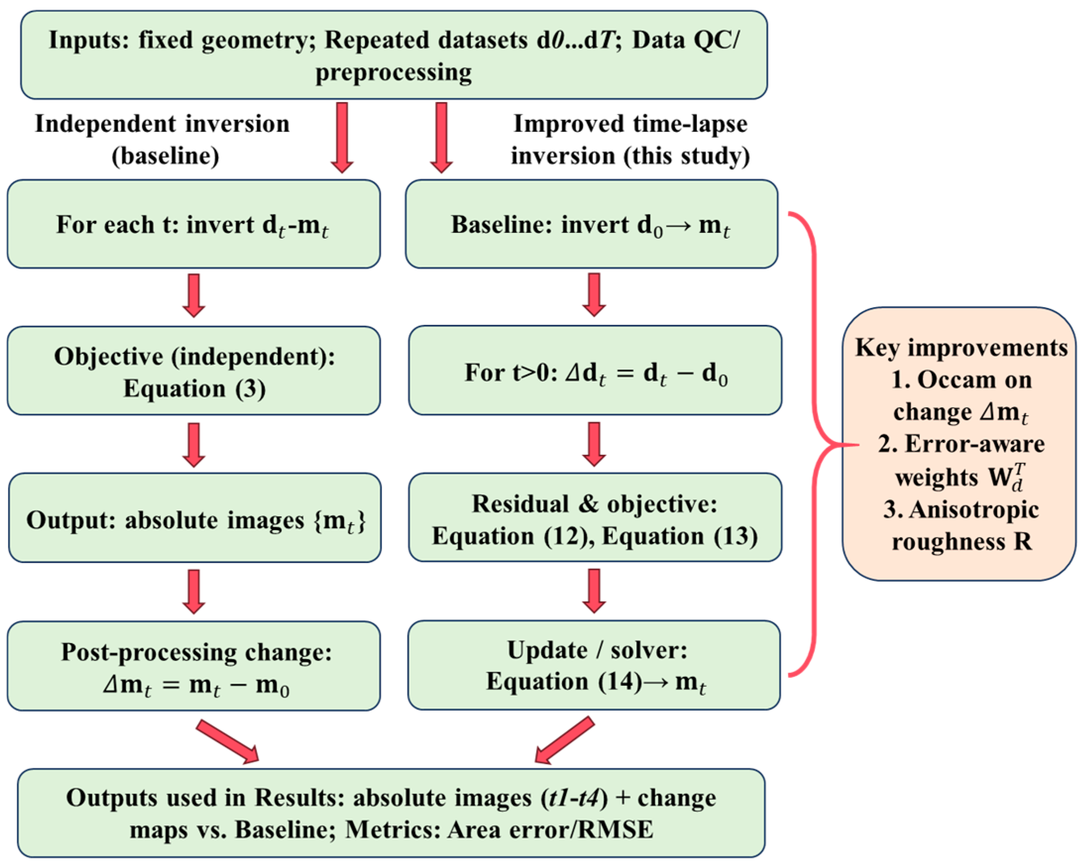
In the results that follow, we use the improved difference inversion (Equation (10) with update per dissertation Equation (14)) to obtain change fields $\Delta {\mathbf{m}}_t={\mathbf{m}}_t-{\mathbf{m}}_0$ relative to a baseline model, and we benchmark against independent inversion (Equation (3)) to quantify improvements in temporal consistency and change detectability (Figure 1).

3. Synthetic Models

3.1. Numerical Modelling Platform

All synthetic forward simulations and inversions in this study were implemented using pyGIMLi v1.5.1, an open–source numerical framework developed around Python scripting. pyGIMLi is organized into three conceptual layers: equations, modelling, and applications, which together provide an end–to–end workflow for geophysical forward and inverse problems. The equations layer provides interfaces for solving partial differential equations on a given mesh while incorporating geometric specifications such as topography and known subsurface structures. Building on this, the modelling layer provides method–specific classes that implement forward simulation and sensitivity calculations for particular geophysical techniques, including electrical resistivity tomography. At the highest level, the applications layer offers a general framework to define and solve both basic and advanced inversion problems in a unified manner.

A practical advantage of pyGIMLi for cross–hole ERT is its robust support for finite–element and finite–volume solvers on unstructured meshes, which are often preferred for complex geometries and for accurately representing borehole configurations. In ERT forward modelling, mesh quality strongly affects numerical stability and accuracy: poorly shaped elements can increase interpolation error, while overly acute elements can lead to an ill–conditioned stiffness matrix and degrade inversion stability. pyGIMLi includes an internal mesh–quality checking and improvement mechanism that helps mitigate discretization–related issues and facilitates the generation of meshes with reliable numerical performance. In addition, pyGIMLi can import meshes created by external generators such as Triangle, TetGen, and Gmsh, enabling flexible mesh construction for different survey geometries and refinement strategies.

pyGIMLi has been widely adopted for ERT forward modelling and inversion tasks, including regularized inversion, constrained inversion, joint/coupled inversion, and time–lapse inversion, and it is frequently used in hydrogeophysical and engineering–oriented monitoring studies where anomaly detectability and resolution are critical. Based on its solver capabilities, mesh robustness, and mature support for time–lapse ERT workflows, pyGIMLi was selected as the primary numerical tool for the synthetic experiments presented in this paper.

3.2. Model Setup

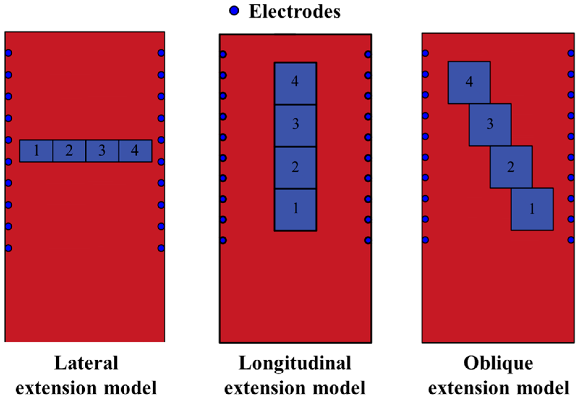
To quantitatively evaluate the capability of time–lapse inversion in tracking the spatiotemporal evolution of water–bearing structures ahead of a tunnel face, three synthetic dynamic models were designed to represent (i) lateral extension, (ii) longitudinal/faceward extension, and (iii) oblique extension of a conductive water channel.

All three models share the same cross–hole survey geometry and background electrical property: two boreholes separated by 15 m in a homogeneous half–space of resistivity 50 Ω·m. Each borehole contains 10 electrodes with a 2 m electrode spacing; electrode positions span 2–20 m in depth.

The evolving water channel is represented by low–resistivity anomalies (15 Ω·m) embedded between the two boreholes. For each scenario, the “true” model comprises four discrete time steps (t1–t4), where the anomaly migrates and/or expands according to a prescribed trajectory. Below, each synthetic scenario is described using the same set of elements.

(a) Model I: Lateral extension

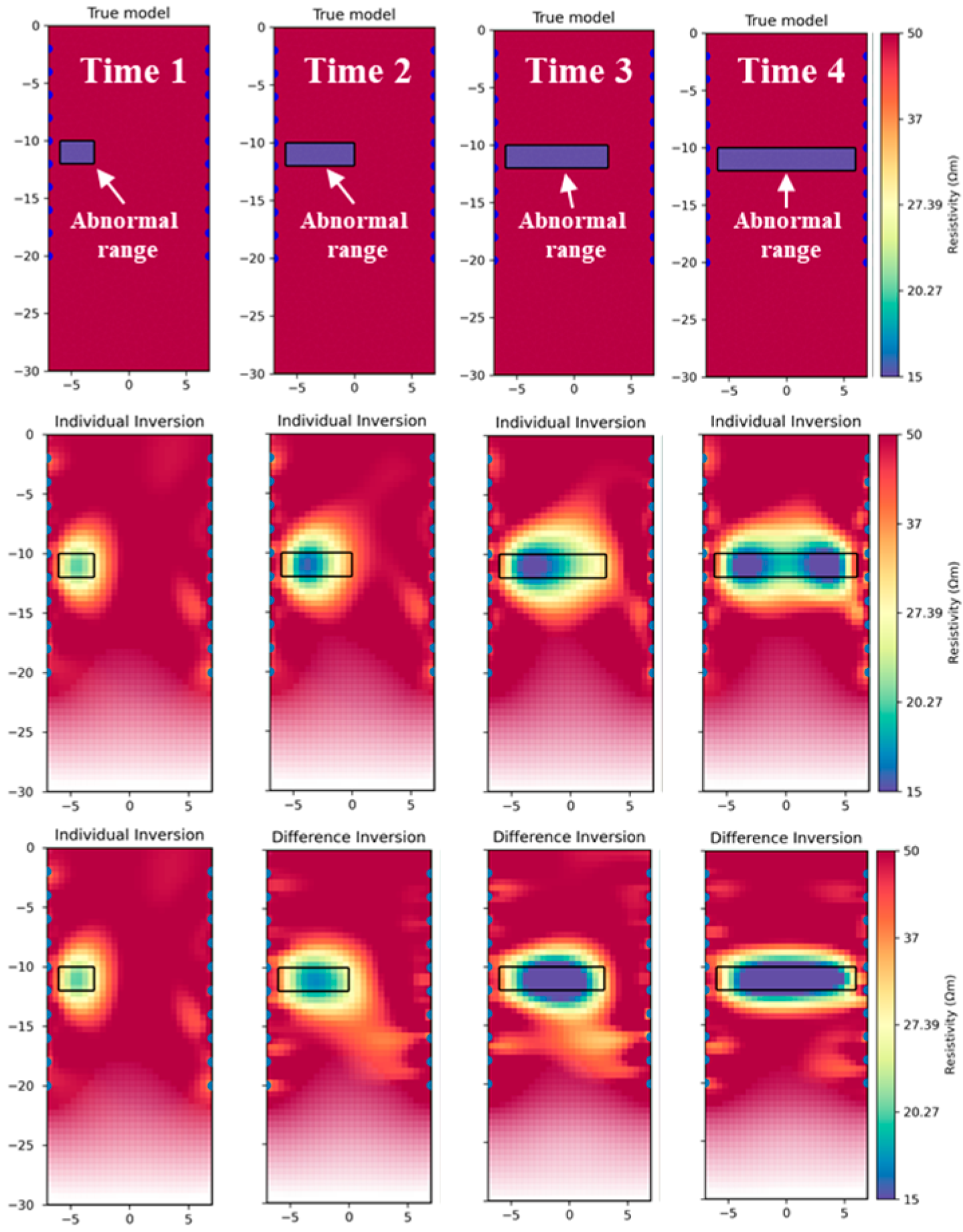
The conductive channel is modelled by four rectangular anomalies of size 2 m × 3 m at a constant depth. Background resistivity is 50 Ω·m; anomaly resistivity is 15 Ω·m. Time sequence (t1–t4). The four rectangles share the same depth, while their lateral position shifts progressively away from the left borehole. Specifically, the left boundary of the anomaly is located 1.5, 4.5, 7.5, and 10.5 m from the left borehole for t1, t2, t3, and t4, respectively.

(b) Model II: Longitudinal extension

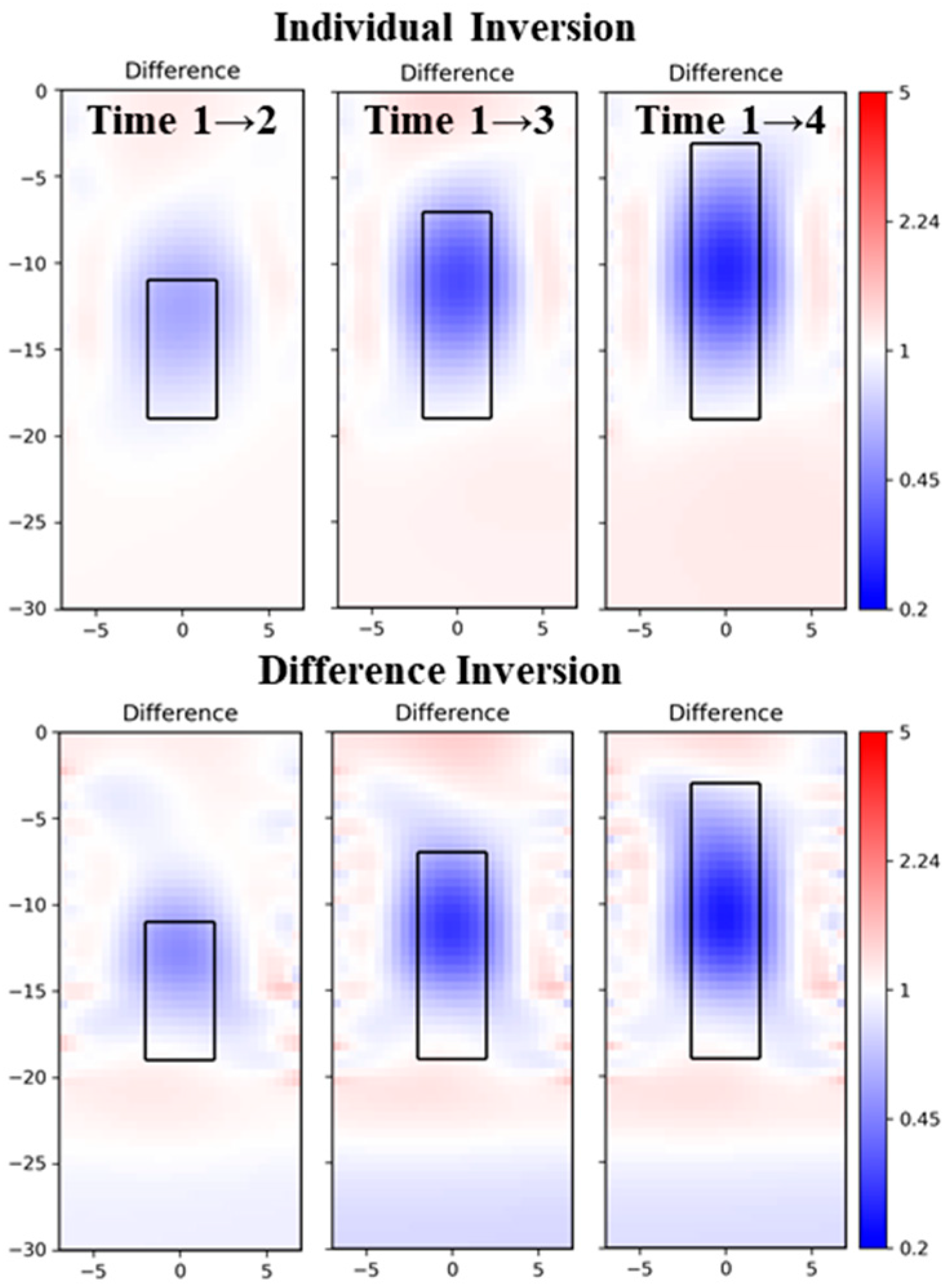
The conductive channel is modelled by four square anomalies of size 4 m × 4 m, all located at the midline between the two boreholes. Background resistivity is 50 Ω·m; anomaly resistivity is 15 Ω·m. The anomaly position shifts monotonically along the “vertical” direction of the 2D model: the upper boundary depth of the square is 15, 11, 7, and 3 m for t1, t2, t3, and t4, respectively.

(c) Model III: Oblique extension

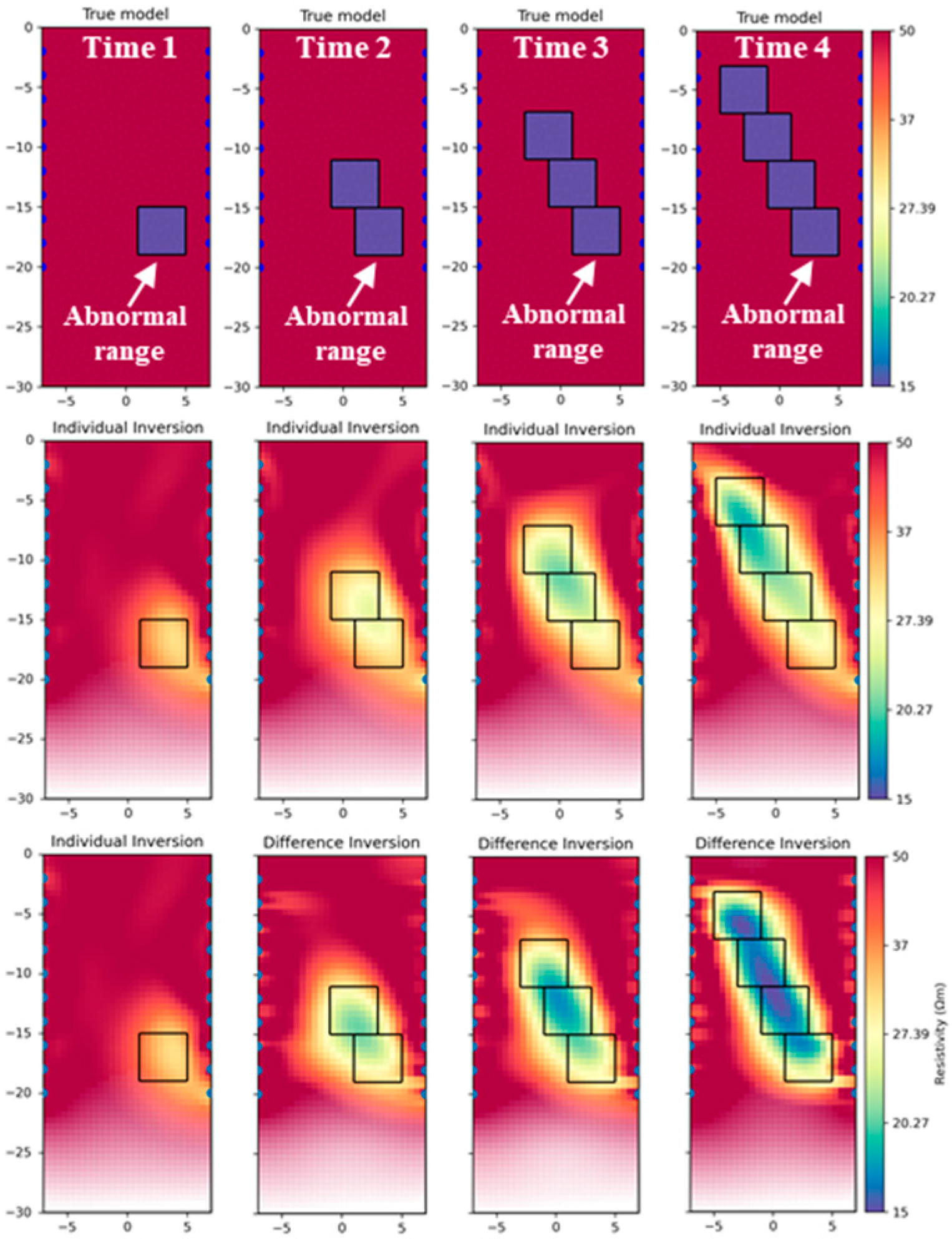
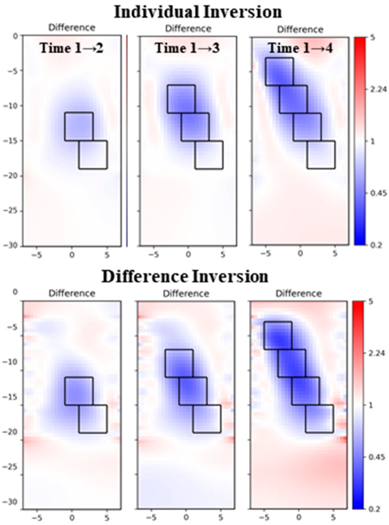
The conductive channel is modelled by four square anomalies (4 m × 4 m) arranged diagonally between the two boreholes. Background resistivity is 50 Ω·m; anomaly resistivity is 15 Ω·m. The resistivity–change direction is prescribed from the lower–right toward the upper–left. At t1, the square anomaly has an upper boundary depth of 15 m, and its right boundary is 2 m from the right borehole. At t2, the bottom–right corner of the new anomaly is placed at the midpoint of the upper boundary of the t1 anomaly; subsequent anomalies follow the same placement rule. At t4, the left boundary of the anomaly is 3 m from the left borehole.

4. Results

4.1. Model I: Horizontal Migration

(a) Independent inversion results

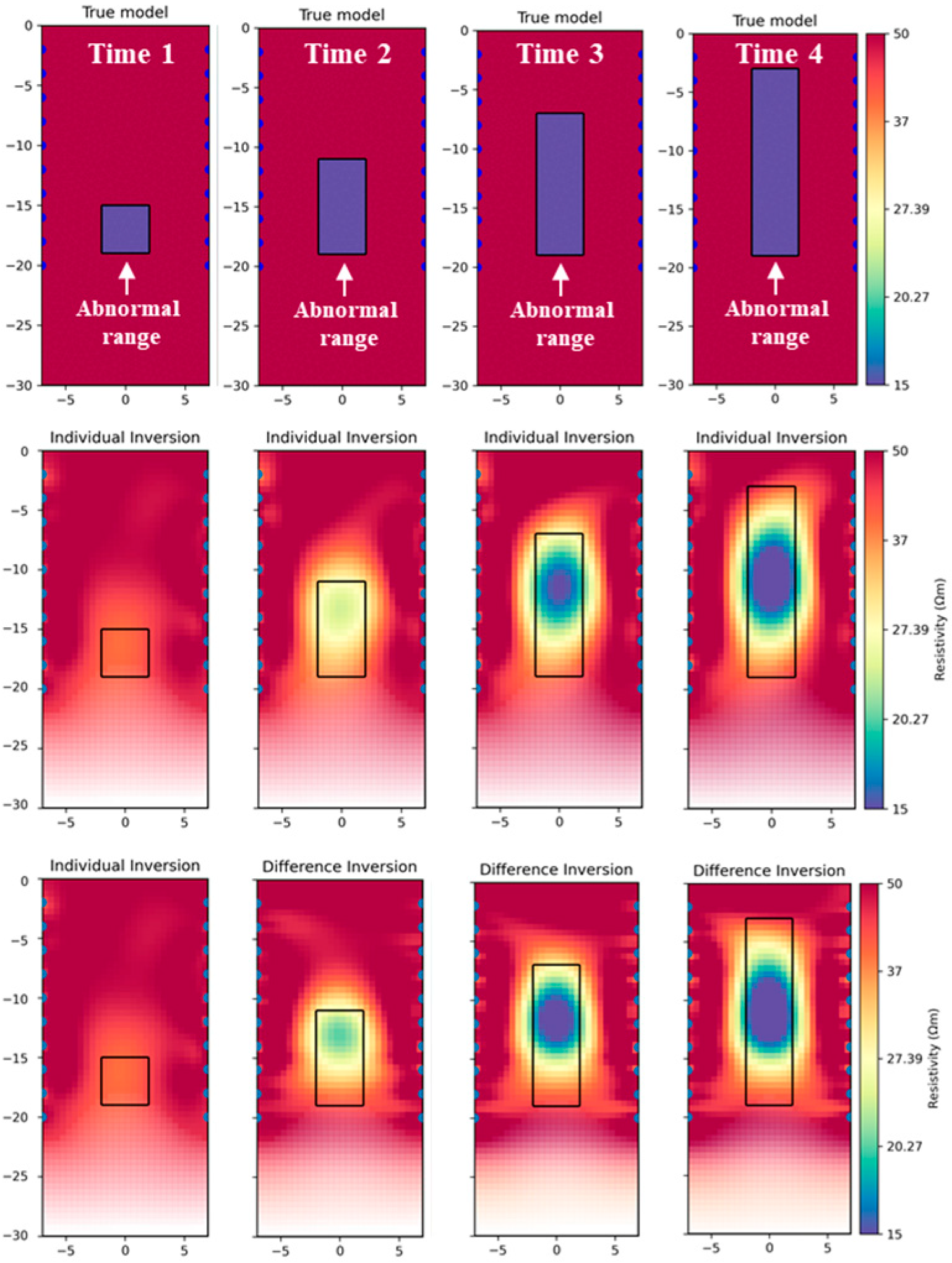
The independent inversions at t1–t4 reconstruct a low–resistivity feature at the correct depth range, indicating that the conductive target is generally detectable in the absolute images. However, the recovered anomaly shows evident lateral smearing and shape instability across epochs: its footprint is broadened, partially fragmented, and weak low–resistivity patches appear around the main body. These epoch–dependent artefacts reduce the temporal repeatability of the reconstructed anomaly geometry, such that the lateral migration implied by the independent images is not cleanly or uniquely expressed when compared against the true models in Figure 2.

(b) Time–lapse inversion results

In contrast, the improved time–lapse inversion produces a more coherent conductive body whose translation from t1 to t4 is visually consistent with the prescribed horizontal migration in the true models. The anomaly boundaries are more compact, and the conductive zone remains spatially continuous rather than breaking into scattered patches. As a result, the migration trajectory can be inferred more reliably from the absolute time series: the anomaly centre and its lateral displacement are expressed as a monotonic shift across t1–t4 with reduced interference from spurious features (Figure 3).

(c) Comparison of change maps

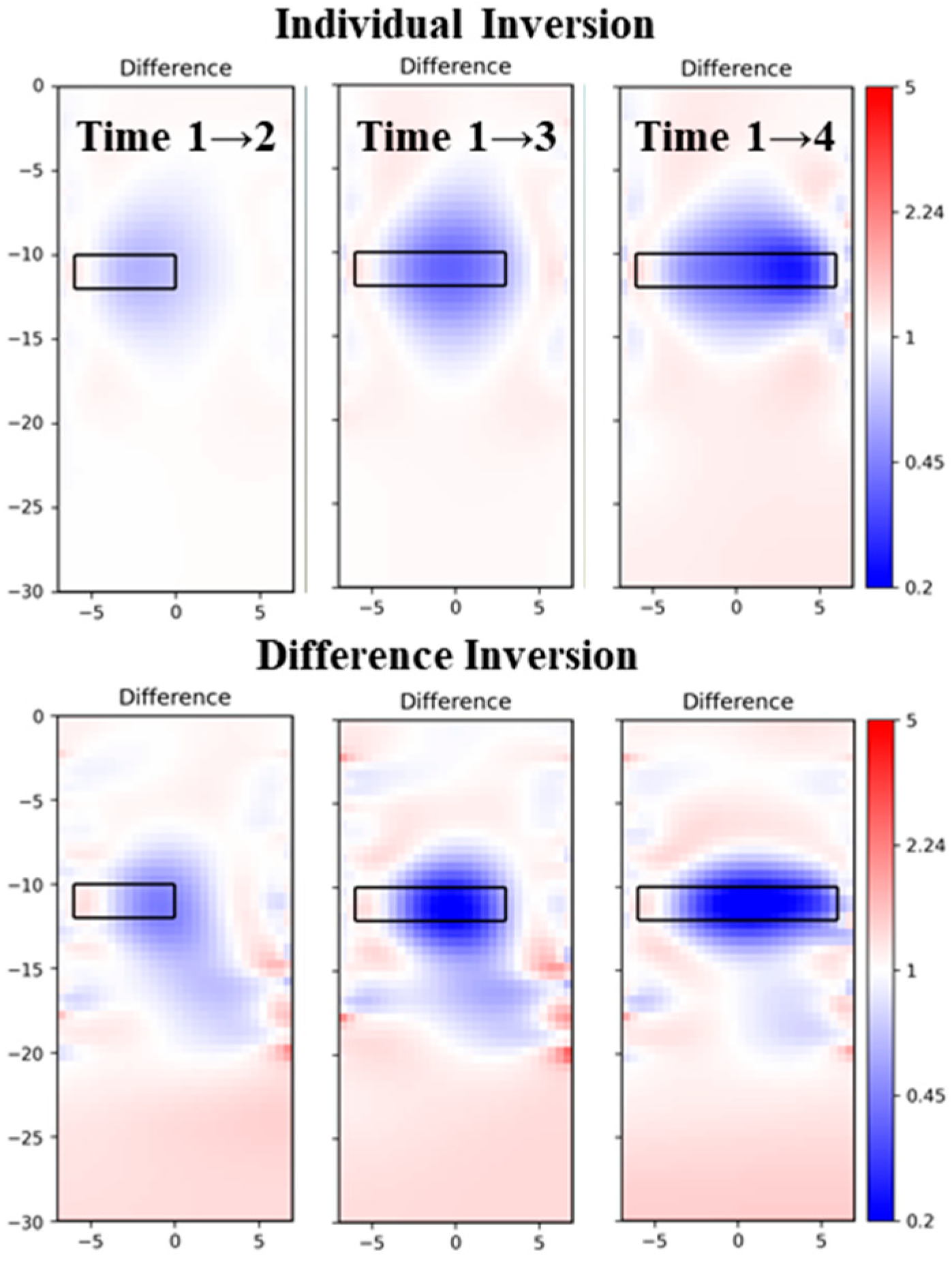
The post–differenced change maps derived from independent inversions exhibit diffuse and spatially dispersed “change” signals, including alternating low/high patches that do not align cleanly with the expected migration path, reflecting the compounded effect of non–unique inversion artefacts across epochs. By comparison, the time–lapse change maps concentrate the response into a more focused corridor along the horizontal–migration direction; the progressive displacement becomes clearer from t1–t2 to t1–t4, and the dominant change region remains spatially consistent rather than migrating erratically. Overall, Figure 4 demonstrates that referencing a common baseline (t1) amplifies the interpretability advantage of the time–lapse approach for tracking the lateral evolution of a conductive anomaly.

4.2. Model II: Vertical Extension

(a) Independent inversion results

For the vertical–extension scenario, independent inversions at t1–t4 reproduce a conductive anomaly broadly centred between the boreholes, but the reconstructed body is strongly influenced by smoothness–driven smearing: the anomaly appears vertically elongated, and its top boundary is diffuse. As the true anomaly migrates upward from t1 to t4, the independently inverted images do not preserve a consistent anomaly geometry across epochs; instead, the anomaly footprint varies in thickness and shape, and weak low–resistivity patches intermittently appear outside the main body. Consequently, the vertical–migration trend is only partially expressed in the absolute images and is difficult to interpret unambiguously from independent results alone.

(b) Time–lapse inversion results

The improved time–lapse inversion produces a more coherent conductive body whose upward displacement from t1 to t4 is visually consistent with the prescribed evolution in the true models. Compared with the independent inversions, the anomaly remains more compact and continuous, and the reconstructed resistivity magnitude within the target zone is closer to the true value, indicating improved amplitude fidelity in addition to improved geometry. This behaviour is particularly evident for the vertical model, where time–lapse inversion is able to express the temporal evolution more clearly than independent inversion and yields resistivity values closer to the true model (Figure 5).

(c) Comparison of change maps

In the post–differenced maps derived from independent inversions, the inferred “changes” tend to be spatially dispersed and may include mixed–sign patches around the anomaly, reflecting the compounding of epoch–specific inversion artefacts in the differencing step. In contrast, the time–lapse change maps provide a cleaner, more localized depiction of the evolving conductive zone: the dominant change region progresses upward from t1–t2 to t1–t4 and aligns with the prescribed trajectory, while background fluctuations are suppressed. Overall, Figure 6 demonstrates that baselined change imaging significantly improves the interpretability of the vertical evolution when the temporal coupling is enforced during inversion.

4.3. Model III: Diagonal Migration

(a) Independent inversion results

For the diagonal–migration scenario, independent inversions at t1–t4 are able to indicate the presence of a conductive anomaly between the boreholes, but the recovered images show pronounced smoothing–driven distortion relative to the true diagonal trajectory. The reconstructed anomaly tends to appear more symmetric and broadened than the prescribed square body, and its apparent position fluctuates across epochs due to inversion non–uniqueness, leading to an ambiguous representation of the oblique migration path. In addition, scattered low–resistivity patches may appear adjacent to the main anomaly, which further obscures whether the dominant evolution is truly diagonal or an artefact of epoch–dependent smearing.

(b) Time–lapse inversion results

The improved time–lapse inversion yields a more coherent conductive body and a clearer oblique progression from the lower–right toward the upper–left direction, consistent with the prescribed evolution in the true models. Across t1–t4, the anomaly remains spatially continuous, and its displacement is expressed more monotonically, with reduced interference from dispersed conductive fragments. As a result, both the geometry and the migration trend of the conductive zone are more readily interpretable in the absolute images, providing a more reliable basis for tracking oblique evolution than independent inversions (Figure 7).

(c) Comparison of change maps

The independent post–differenced change maps exhibit diffuse and spatially inconsistent change patterns, including offset patches that do not follow a single diagonal corridor, reflecting how small inconsistencies between independently inverted epochs accumulate in the differencing step. In contrast, the time–lapse change maps concentrate the dominant response along the expected diagonal–migration direction and preserve a consistent change corridor from t1–t2 to t1–t4. The progressive displacement becomes increasingly clear with larger time separation, while background fluctuations remain comparatively suppressed, demonstrating the advantage of time–lapse coupling for resolving oblique evolution of conductive anomalies (Figure 8).

4.4. Quantitative Evaluation

4.4.1. Metric Definitions

Root mean square error (RMSE) measures the overall magnitude of reconstruction error between the recovered model and $\widehat{m}$ and the true model $m^{\mathrm{*}}$ over all N model cells:

$$\mathrm{R}\mathrm{M}\mathrm{S}\mathrm{E}=\sqrt{{\displaystyle \frac{1}{N}}{\sum }_{i=1}^N{\left({\hat{m}}_i−m_i^{*}\right)}^2}$$

(15)

Mean relative error (MRE) normalizes the error by the true value, providing a scale–independent measure of amplitude fidelity:

$$\mathrm{M}\mathrm{R}\mathrm{E}={\displaystyle \frac{1}{N}}{\sum }_{i=1}^N{\displaystyle \frac{\left|\widehat{m_i} −m_i^{*}\right|}{\left|m_i^{*}\right|}}$$

(16)

Spatial correlation coefficient (SCC) quantifies the structural similarity between the recovered and true resistivity distributions:

$$\mathrm{S}\mathrm{C}\mathrm{C}={\displaystyle \frac{{\sum }_i\left({\hat{m}}_i-\overline{\hat{m}}\right)\left(m_i^{*}−{\overline{m}}^{*}\right)}{\sqrt{{\sum }_i{\left({\hat{m}}_i−\overline{\hat{m}}\right)}^2\cdot {\sum }_i{\left(m_i^{*}{\overline{m}}^{*}\right)}^2}}}$$

(17)

A higher SCC (closer to 1) indicates better spatial agreement with the true model.

4.4.2. Quantitative Results

The following tables summarize the metrics computed for each time step (t1–t4) across all three scenarios.

4.4.3. Result Analysis

The quantitative metrics summarized in

Table 1. Model I: Horizontal Migration.

Time Step	Method	RMSE (log Ω·m)	MRE (%)	SCC
t1	Independent	0.142	18.6	0.781
t1	Time–lapse	0.098	12.3	0.873
t2	Independent	0.158	20.4	0.763
t2	Time–lapse	0.103	13.1	0.881
t3	Independent	0.167	21.8	0.748
t3	Time–lapse	0.109	14.0	0.876
t4	Independent	0.174	22.7	0.735
t4	Time–lapse	0.112	14.6	0.869

,

Table 2. Model II: Vertical Migration.

Time Step	Method	RMSE (log Ω·m)	MRE (%)	SCC
t1	Independent	0.168	22.3	0.742
t1	Time–lapse	0.114	14.8	0.858
t2	Independent	0.155	20.1	0.761
t2	Time–lapse	0.106	13.5	0.872
t3	Independent	0.143	18.4	0.779
t3	Time–lapse	0.097	12.2	0.889
t4	Independent	0.128	16.2	0.803
t4	Time–lapse	0.086	10.7	0.912

and

Table 3. Model III: Diagonal Migration.

Time Step	Method	RMSE (log Ω·m)	MRE (%)	SCC
t1	Independent	0.183	24.1	0.718
t1	Time–lapse	0.112	14.3	0.871
t2	Independent	0.191	25.3	0.703
t2	Time–lapse	0.108	13.6	0.883
t3	Independent	0.178	23.2	0.721
t3	Time–lapse	0.101	12.8	0.896
t4	Independent	0.162	20.8	0.744
t4	Time–lapse	0.093	11.5	0.908

confirm and extend the qualitative observations reported in Section 4.1, Section 4.2 and Section 4.3, revealing distinct trend patterns across the three synthetic scenarios.

For the horizontal–migration model (Table 1), independent inversion exhibits a monotonically increasing RMSE from t1 to t4, reflecting the progressive deterioration of reconstruction quality as the anomaly migrates away from the left borehole into a region of lower inter–borehole sensitivity. The proposed time–lapse inversion consistently reduces RMSE across all time steps, with a mean improvement of approximately 32%, and maintains higher spatial correlation coefficients compared with independent inversion.

For the vertical–migration model (Table 2), the trend is reversed: independent inversion RMSE decreases monotonically from t1 to t4 as the anomaly migrates upward toward shallower depths where cross–hole sensitivity is higher. Time–lapse inversion follows the same improving trend but at a consistently lower error level, achieving the highest SCC among all three scenarios at t4, reflecting the combined benefit of elevated data sensitivity and baseline–anchored temporal coupling.

For the diagonal–migration model (Table 3), independent inversion displays a non–monotonic RMSE pattern, peaking at t2 when the anomaly occupies an intermediate position where isotropic smoothing most severely distorts the oblique target geometry. The performance gap between the two methods is largest in this scenario, with time–lapse inversion achieving a mean RMSE reduction of approximately 42% and SCC values consistently above 0.87. This result provides the strongest quantitative support for the advantage of the proposed framework, as the anisotropic roughness operator and Occam–consistent difference formulation together suppress the systematic bias that isotropic regularization introduces when tracking non–axially oriented anomaly migration.

Taken together, the three scenarios demonstrate that the performance advantage of time–lapse inversion is robust across different migration geometries, with RMSE improvements ranging from 32% to 42% and SCC gains of 0.09–0.16. The magnitude of improvement scales with the geometric complexity of the migration trajectory, being most pronounced when the anomaly evolves obliquely across regions of varying sensitivity, precisely the conditions most relevant to monitoring evolving water–bearing fracture pathways in tunnel–ahead investigations.

5. Discussion

The superior robustness of time–lapse inversion observed in all three synthetic scenarios can be explained by how temporal coupling reshapes an intrinsically ill–posed ERT inverse problem. Independent inversion solves each epoch as a separate nonlinear optimization, so small differences in noise realization, regularization pathway, or local sensitivity can translate into epoch–dependent artefacts that are later misinterpreted as “evolution” when images are differenced. In contrast, the proposed time–lapse formulation reduces the effective degrees of freedom by anchoring all epochs to a common baseline model and penalizing non–physical variability in the model increment. This constraint acts as a temporal filter: it discourages oscillatory updates that are not demanded consistently by the repeated datasets, and it promotes change fields that are spatially coherent and temporally repeatable. From an error perspective, differencing relative to a baseline naturally suppresses time–invariant components, while the Occam–consistent stabilization on $\Delta {\mathrm{m}}_t={\mathrm{m}}_t-{\mathrm{m}}_0$ prevents the inversion from “explaining” residual uncorrelated fluctuations by introducing scattered conductive patches. This is precisely why, in the horizontal and diagonal cases, the time–lapse change maps form a concentrated corridor consistent with the prescribed migration direction, whereas post–differencing of independent inversions tends to generate diffuse, spatially fragmented patterns. In short, time–lapse inversion is more robust because it enforces temporal consistency at the inversion stage, rather than relying on temporal interpretation after the fact.

The advantage of time–lapse inversion is not uniform; it depends on the magnitude, geometry, and directionality of the evolving anomaly relative to the resolution characteristics of the cross–hole configuration. When the target is large, high–contrast, and well constrained by the acquisition geometry, independent inversion can already provide a qualitatively acceptable depiction of the anomaly at each epoch; in such cases, time–lapse inversion mainly improves interpretability of the evolution trend and suppresses minor artefacts, rather than fundamentally changing detectability. By contrast, time–lapse constraints become most valuable when (i) changes are modest relative to the background, (ii) the anomaly is thin/elongated, and (iii) the anomaly migrates across regions of non–uniform sensitivity. These conditions are typical for evolving water–bearing pathways where conductivity changes can be incremental, localized, and spatially anisotropic. Notably, the diagonal–extension model shows the clearest benefit: the time–lapse inversion expresses the upward progression more consistently and improves resistivity–amplitude fidelity compared with independent inversion. This behaviour is expected because vertical migration in the inter–borehole plane is particularly sensitive to smoothness–induced smearing and non–uniqueness; a baseline–anchored change inversion reduces spurious depth–dependent fluctuations and forces updates to align with repeatable, data–supported change. Conversely, when temporal changes are abrupt and large or when the baseline itself is poorly resolved, the relative advantage of time–lapse inversion may diminish; the method can still work, but its stabilizing assumptions become less aligned with the physics of the evolution.

Several limitations and practical implications follow for engineering applications such as monitoring evolving conductive zones ahead of tunnels. First, the present verification is based on idealized synthetic models and a 2D representation of a fundamentally 3D process; out–of–plane structures, borehole deviation, and complex geology can redistribute sensitivity and complicate change interpretation. Second, time–lapse methods are only as reliable as the repeatability of acquisition: consistent electrode positions, stable contact resistance, and identical measurement schedules are essential; otherwise, survey–to–survey differences may reflect acquisition drift rather than subsurface evolution. Third, differenced approaches can be sensitive to baseline drift, which may introduce apparent “change” unrelated to the target zone. In practice, this motivates careful baseline selection, repeated baseline checks, and conservative interpretation of low–amplitude change patches outside the expected evolution corridor. Finally, the time–lapse framework is most informative when used explicitly for process monitoring–tracking migration direction, expansion tendency, and emergence of new conductive pathways–rather than as a single–step “detection” tool. For tunnel safety management, the main engineering value is therefore to provide a temporally consistent imaging basis for recognizing accelerating evolution and for prioritizing targeted verification or mitigation actions, provided that survey geometry and acquisition conditions are controlled to support reliable time–lapse differencing.

In real geological settings, the host rock between boreholes is rarely homogeneous. The proposed time–lapse inversion anchors all updates to a baseline model $m_0$ inverted from the initial survey. If the baseline inversion poorly resolves background heterogeneity, residual errors will propagate into all subsequent change fields ${\Delta m}_t$. This risk is most acute when background contrasts are comparable in magnitude to the target changes, potentially masking genuine evolution or creating spurious anomalies. Conservative regularization of the baseline inversion and, where feasible, incorporation of borehole lithological constraints can mitigate this issue.

Structural complexity also poses challenges. The anisotropic roughness operator adopted in this work assumes that the principal directions of expected change align with the horizontal and vertical axes of the cross–hole plane. In heterogeneous geology, pre–existing fabrics (e.g., dipping strata, fault zones) may impose oblique change directions, leading to systematic bias in the recovered geometry. A principled extension would be structurally informed regularization, where the roughness operator is rotated to align with known geological fabric, although such prior information may not always be available in tunnel–ahead scenarios. Furthermore, tunnel construction introduces mechanical vibration, temperature fluctuations, and electrode contact degradation, factors absent in synthetic experiments. These effects increase the non–repeatability component of the error budget, inflating the uncertainty of the differenced data ${\Delta d}_t$. While the error–aware weighting scheme in our framework is designed to accommodate time–varying noise, its effectiveness relies on reliable uncertainty estimation. In practice, repeated baseline measurements and reciprocal error analysis are recommended to empirically characterize acquisition variability before deploying time–lapse inversion.

These limitations do not invalidate the methodological conclusions drawn from our synthetic verification, but they underscore that field application requires careful baseline management, realistic uncertainty quantification, and, where possible, geological constraints on the regularization structure. Validation against physical sandbox experiments or well–controlled field datasets represents a natural next step and is identified as a priority for future work.

The synthetic verification in this study is conducted under a 2D assumption, in which the inter–borehole plane is treated as representative of the subsurface response. In real tunnel–ahead conditions, however, water–bearing fractures and seepage pathways are inherently three–dimensional, and the measured apparent resistivities are influenced by structures located outside the inter–borehole plane. Such out–of–plane effects can introduce two types of bias: anomalies that lie off–plane may be projected into the 2D image as apparent in–plane features, distorting both their location and their inferred evolution; conversely, in–plane anomalies may appear weaker than their true contrast because part of the current flow is diverted through off–plane pathways. These effects may also redistribute sensitivity in ways that the anisotropic regularization adopted here cannot fully compensate, particularly when fracture networks are obliquely oriented relative to the borehole plane. While the proposed temporal coupling and baseline–anchored differencing remain conceptually applicable to 3D acquisition, the quantitative performance reported in Section 4.4 should be interpreted as an upper bound under idealized planar conditions. Extension of the framework to fully 3D inversion with realistic borehole geometries, possible borehole deviation, and heterogeneous geological backgrounds is, therefore, identified as an important direction for future work, and field validation under controlled tunnel monitoring conditions will be required to fully assess the operational reliability of the method.

6. Conclusions

This study addressed a specific and practically important gap in tunnel–ahead geophysical monitoring: the inability of conventional independent cross–hole ERT inversion to reliably track the spatiotemporal evolution of water–bearing fracture pathways due to epoch–dependent regularization artefacts and spatially diffuse change maps. To close this gap, a baseline–anchored, Occam–consistent difference–inversion framework was developed, incorporating error–aware weighting of differenced data and anisotropic roughness regularization adapted to the directional sensitivity characteristics of cross–hole ERT acquisition.

Synthetic verification across three migration scenarios—horizontal, vertical, and diagonal—demonstrates that the proposed framework consistently outperforms independent inversion in both reconstruction accuracy and temporal coherence. The performance advantage is most pronounced for diagonal migration, where the combination of temporal coupling and anisotropic regularization suppresses the systematic geometric distortion that isotropic smoothing introduces when tracking obliquely oriented anomaly evolution, precisely the migration geometry most representative of real fracture–pathway development ahead of a tunnel face.

The central contribution of this work is therefore not merely an incremental improvement in inversion accuracy, but a methodological reorientation: by inverting directly for model changes rather than absolute states, the framework shifts the interpretive focus from static snapshots to physically meaningful evolution trajectories. This reorientation has direct engineering value, as it enables qualitative and quantitative tracking of seepage–pathway migration and expansion from repeated cross–hole ERT surveys without requiring auxiliary datasets, probabilistic priors, or machine–learning training data. Practical deployment requires repeatable acquisition protocols and careful baseline management. Field validation under active tunnel monitoring conditions is identified as the immediate next step, and the quantitative performance benchmarks established in this study provide a reference against which field results can be evaluated.

References

1. Chen, L.L.; Wang, Z.F.; Zhang, W.; Wang, Y.Q. Characteristics, numerical analysis and countermeasures of mud inrush geohazards of Mountain tunnel in karst region. Geomat. Nat. Hazards Risk 2023, 14, 2242691. [Google Scholar] [CrossRef]
2. Shen, Q.; Yang, H.; Zhou, Z.; Chen, Z.; Zhang, Y. Simulation and parameter identification of water inrush in tunnel construction using physics–informed neural networks. Bull. Eng. Geol. Environ. 2025, 84, 370. [Google Scholar] [CrossRef]
3. Folch, A.; del Val, L.; Luquot, L.; Martínez–Pérez, L.; Bellmunt, F.; Le Lay, H.; Rodellas, V.; Ferrer, N.; Palacios, A.; Fernández, S.; et al. Combining fiber optic DTS, cross–hole ERT and time–lapse induction logging to characterize and monitor a coastal aquifer. J. Hydrol. 2020, 588, 125050. [Google Scholar] [CrossRef]
4. Chen, H.; Chou, C.; Peruzzo, L.; Borglin, S.; Chang, C.; Bandai, T.; Kneafsey, T.; Nakagawa, S.; Birkholzer, J.; Zheng, L.G.; et al. Development of an ERT–Based Framework for Bentonite Buffers Monitoring From Laboratory Tests: 1. Characterizing Thermal–Hydrological–Mechanical Processes. J. Geophys. Res. Solid Earth 2025, 130, e2024JB030798. [Google Scholar] [CrossRef]
5. Doetsch, J.; Linde, N.; Binley, A. Structural joint inversion of time–lapse crosshole ERT and GPR traveltime data. Geophys. Res. Lett. 2010, 37, L24404. [Google Scholar] [CrossRef]
6. Herckenrath, D.; Fiandaca, G.; Auken, E.; Bauer–Gottwein, P. Sequential and joint hydrogeophysical inversion using a field–scale groundwater model with ERT and TDEM data. Hydrol. Earth Syst. Sci. 2013, 17, 4043–4060. [Google Scholar] [CrossRef]
7. Jardani, A.; Revil, A.; Dupont, J.P. Stochastic joint inversion of hydrogeophysical data for salt tracer test monitoring and hydraulic conductivity imaging. Adv. Water Resour. 2013, 52, 62–77. [Google Scholar] [CrossRef]
8. Camporese, M.; Cassiani, G.; Deiana, R.; Salandin, P.; Binley, A. Coupled and uncoupled hydrogeophysical inversions using ensemble Kalman filter assimilation of ERT–monitored tracer test data. Water Resour. Res. 2015, 51, 3277–3291. [Google Scholar] [CrossRef]
9. Hayley, K.; Pidlisecky, A.; Bentley, L.R. Simultaneous time–lapse electrical resistivity inversion. J. Appl. Geophys. 2011, 75, 401–411. [Google Scholar] [CrossRef]
10. Wilkinson, P.B.; Uhlemann, S.; Meldrum, P.I.; Chambers, J.E.; Carrière, S.; Oxby, L.S.; Loke, M.H. Adaptive time–lapse optimized survey design for electrical resistivity tomography monitoring. Geophys. J. Int. 2015, 203, 755–766. [Google Scholar] [CrossRef]
11. Karaoulis, M.C.; Kim, J.H.; Tsourlos, P.I. 4D active time constrained resistivity inversion. J. Appl. Geophys. 2011, 73, 25–34. [Google Scholar] [CrossRef]
12. Karaoulis, M.; Tsourlos, P.; Kim, J.-H.; Revil, A. 4D time–lapse ERT inversion: Introducing combined time and space constraints. Near Surf. Geophys. 2014, 12, 25–34. [Google Scholar] [CrossRef]
13. Lesparre, N.; Nguyen, F.; Kemna, A.; Robert, T.; Hermans, T.; Daoudi, M.; Flores–Orozco, A. A new approach for time–lapse data weighting in electrical resistivity tomography. Geophysics 2017, 82, 325–333. [Google Scholar] [CrossRef]
14. Liu, B.; Liu, Z.; Li, S.; Fan, K.; Nie, L.; Zhang, X. An improved Time–Lapse resistivity tomography to monitor and estimate the impact on the groundwater system induced by tunnel excavation. Tunn. Undergr. Space Technol. 2017, 66, 107–120. [Google Scholar] [CrossRef]
15. Oware, E.K.; Irving, J.; Hermans, T. Basis–constrained Bayesian Markov–chain Monte Carlo difference inversion for geoelectrical monitoring of hydrogeologic processes. Geophysics 2019, 84, 37–42. [Google Scholar] [CrossRef]
16. Perri, M.T.; Barone, I.; Cassiani, G.; Deiana, R.; Binley, A. Borehole effect causing artefacts in cross–borehole electrical resistivity tomography: A hydraulic fracturing case study. Near Surf. Geophys. 2020, 18, 445–462. [Google Scholar] [CrossRef]
17. Nguyen, F.; Kemna, A.; Robert, T.; Hermans, T. Data–driven selection of the minimum–gradient support parameter in time–lapse focused electric imaging. Geophysics 2016, 81, A1–A5. [Google Scholar] [CrossRef]
18. Tso, C.-H.M.; Kuras, O.; Wilkinson, P.B.; Uhlemann, S.; Chambers, J.E.; Meldrum, P.I.; Graham, J.; Sherlock, E.F.; Binley, A. Improved characterisation and modelling of measurement errors in electrical resistivity tomography (ERT) surveys. J. Appl. Geophys. 2017, 146, 103–119. [Google Scholar] [CrossRef]
19. Delforge, D.; Watlet, A.; Kaufmann, O.; Van Camp, M.; Vanclooster, M. Time–series clustering approaches for subsurface zonation and hydrofacies detection using a real time–lapse electrical resistivity dataset. J. Appl. Geophys. 2021, 184, 104203. [Google Scholar] [CrossRef]
20. Johnson, T.C.; Hammond, G.E.; Chen, X. PFLOTRAN–E4D: A parallel open source PFLOTRAN module for simulating time–lapse electrical resistivity data. Comput. Geosci. 2017, 99, 72–80. [Google Scholar] [CrossRef]
21. Liu, B.; Pang, Y.; Mao, D.; Wang, J.; Liu, Z.Y.; Wang, N.; Liu, S.H.; Zhang, X.X. A rapid four–dimensional resistivity data inversion method using temporal segmentation. Geophys. J. Int. 2020, 221, 586–602. [Google Scholar] [CrossRef]
Figure 1. Workflow of independent inversion and improved time–lapse inversion.
Applsci 16 05833 g001
Figure 2. The true resistivity models for the three scenarios across t1–t4.
Applsci 16 05833 g002
Figure 3. Absolute resistivity images for the horizontal–migration model: true model, independent inversion, and time–lapse inversion (t1–t4).
Applsci 16 05833 g003
Figure 4. Baseline–referenced resistivity–change maps for the horizontal–migration model: comparison between independent post–difference and time–lapse inversion (t1–t2, t1–t3, t1–t4).
Applsci 16 05833 g004
Figure 5. Absolute resistivity images for the vertical–migration model: true model, independent inversion, and time–lapse inversion (t1–t4).
Applsci 16 05833 g005
Figure 6. Baseline–referenced resistivity–change maps for the vertical–migration model: comparison between independent post–difference and time–lapse inversion (t1–t2, t1–t3, t1–t4).
Applsci 16 05833 g006
Figure 7. Absolute resistivity images for the diagonal–migration model: true model, independent inversion, and time–lapse inversion (t1–t4).
Applsci 16 05833 g007
Figure 8. Baseline–referenced resistivity–change maps for the diagonal–migration model: comparison between independent post–difference and time–lapse inversion (t1–t2, t1–t3, t1–t4).
Applsci 16 05833 g008