An Advanced Method of Modeling the Dynamics of a Suspended Monorail Using Fractal Analysis

Abstract

Fractional differential operators provide an effective approach for modeling complex technological processes, particularly physical phenomena in continuum mechanics characterized by memory and non-local effects. Different types of fractional derivatives require different numerical approximation schemes; in this study, the Caputo and Grünwald–Letnikov derivatives are considered. The aim of this work was to develop and validate a fractional differential model of longitudinal oscillations in a suspended monorail system that accounts for nonlinear and memory-dependent effects. In contrast to classical integer-order approaches, the proposed framework incorporates multiscale surface irregularity effects, including rail roughness, friction, and other disturbances influencing system dynamics, through a fractional-order formulation. A fractional differential mathematical model describing the motion of longitudinal oscillations of a large-sized cargo transported along a suspended monorail is proposed. A numerical algorithm based on finite-difference approximation of fractional operators was developed for its implementation. The scientific contribution lies in integrating multiscale surface irregularity effects into a fractional-order modeling framework to improve the accuracy of dynamic response prediction. Numerical experiments demonstrated the effectiveness of the approach, and the results were validated through comparison with existing models of monorail dynamics. Additionally, statistical validation based on correlation analysis confirmed good agreement with the experimental data. The proposed model can be applied to the design and optimization of suspended transport systems, improving vibration control, reliability, and operational safety under real dynamic loading conditions.

1. Introduction

1.1. Works on Fractional and Fractal Modeling

Fractional differential operators provide an effective approach to modeling complex technological processes, in particular, physical phenomena in continuous media mechanics (continuum mechanics). The use of fractal operators for modeling complex systems makes it possible to take into account non-local interactions, “memory” effects, and anomalous diffusion processes that cannot be described by traditional methods. In [1], the authors describe how fractal properties—such as self-similarity, complexity, and nonlinearity—can be used for data analysis, classification, recognition, and compression. In [2], fractal analysis was investigated for the capability of differentiating benign from malignant thyroid nodules during ultrasonography. The work [3] deals with experimental and numerical studies of heat distribution in the external partition of a building, where a mathematical model is formulated on the basis of a fractional differential equation. Studies in [4] have shown the effectiveness of fractional models in describing anomalous diffusion, in particular subdiffusive and superdiffusive processes. In [5], the application of fractional operators for modeling energy losses in nonlinear materials with frequency dependences is demonstrated. This approach proved to be useful in the development of energy-efficient materials and systems with fractal geometry. Practical applications of fractal operators include modeling in the power industry [6], prediction of crack formation in composite materials [7,8], analysis of relaxation processes in materials [9,10], and optimization of technological processes in industry [11]. In particular, works [10,12] emphasize the importance of fractional models which are used for predicting the formation of cracks and analyzing the stress–strain state in composites and biological tissues. Reference [13] presents a descriptive model that characterizes the process of heat and moisture transfer in materials with a fractal structure. Taking into account that the fractional parameters of fractal models allow the deformation–relaxation processes in biomaterials to be described in comparison with traditional methods, the optimal approximation method, the Proni’s method, was proposed more fully in paper [14].

Fractional derivatives are a major component of models with fractal operators. Today, there are different types of fractional derivatives that allow modeling phenomena with different physical properties. At the same time, the existence of different approaches in defining fractional derivatives causes ambiguity in choosing the correct initial and boundary conditions. Since different types of fractional operators have different mathematical properties and physical interpretations, the formulation of the problem can vary significantly depending on the chosen definition of the derivative. This is especially important in applied problems, where the physical meaningfulness of the results plays a key role in correctly describing the evolution of the processes. The work [15] investigates the use of biorthogonal expansion for the calculation of fractional derivatives in the Caputo and Riemann–Liouville terms with respect to accuracy and rate of convergence. Thus, the Riemann–Liouville fractional derivative in its classical form is used for problems with non-local effects [1,16] and has a wide range of applications in subdiffusion models [4].

In this work, the term “fractal” is not used as a reference to a specific mathematical fractal analysis technique, but rather to describe the multiscale and irregular nature of the rail surface geometry. The resulting dynamics are modeled using fractional calculus, which provides a mathematical framework for memory and non-local effects induced by such irregularities.

1.2. Related Works

Currently, there is a limited number of scientific publications that deal with the application of fractal analysis for modeling the movement of monorail transport. However, fractal analysis is widely used in transportation research and vehicle traffic modeling, in particular for the analysis of vehicle dynamics, including modeling road irregularities and their impact on motion [17,18,19,20,21,22], as well as for studying traffic flow characteristics, including scale properties, self-organization, and nonlinear behavior.

In addition, a number of related studies have applied advanced mathematical and computational approaches to transport systems. For example, stochastic and nonlinear dynamic models are used to describe vehicle–track interaction under irregular excitation, while multi-body system dynamics approaches enable detailed analysis of vehicle motion considering suspension systems and external disturbances [23,24]. Numerical methods, including finite element and finite difference techniques, are widely applied for simulating structural vibrations and the dynamic response of transport systems. Furthermore, recent studies explored data-driven and hybrid approaches, including machine learning methods for traffic prediction and system identification, allowing the modeling of complex nonlinear dependencies [25,26].

Existing models often do not fully account for nonlinear effects, rail irregularities, and memory-dependent behavior that arise under real operating conditions. This indicates the need to develop more advanced models that can adequately describe real operating conditions.

The aim of this study was to develop and validate a fractional differential model of longitudinal oscillations of a large-sized cargo transported along a suspended monorail system, taking into account nonlinear interactions and memory effects.

The scientific novelty of the work lies in the integration of fractal analysis with fractional differential operators (Caputo and Grünwald–Letnikov) and in the development of a numerical algorithm based on finite-difference approximation, which enables more accurate prediction of the oscillatory processes compared to traditional approaches.

The practical significance of the obtained results consists in the possibility of their application in the design and optimization of suspended transport systems, in particular for more accurate prediction and control of vibration levels, increasing structural reliability, and improving operational safety under dynamic loading conditions.

Modern approaches to the analysis and optimization of transportation structures demonstrate a clear trend toward the integration of multiphysics models, lightweight composite materials, and digital monitoring technologies. In particular, the work [27] proposed a multi-stage topology optimization approach for the structural redesign of railway locomotive bogie frames, enabling a significant reduction in structural mass while maintaining mechanical strength characteristics. Similarly, the work [28] investigated the potential of lightweight pultruded GFRP fabric panels for railway vehicles, emphasizing the importance of accounting for anisotropy and the complex internal structure of composite materials in dynamic loading problems.

In this context, the concept of a physical digital twin for monitoring railway structures becomes particularly relevant, as it enables the integration of experimental data with real-time numerical simulations, thereby improving the accuracy of state prediction and the remaining lifetime estimation. Additionally, approaches to the experimental validation of complex dynamic systems, particularly in the fields of additive manufacturing and high-temperature gas turbine components, highlight the importance of incorporating nonlinear dynamics, material memory effects, and energy dissipation mechanisms.

The fractional differential model of the suspended monorail system proposed in this study is consistent with these current trends, as it naturally accounts for memory effects, viscoelastic behavior of composite elements, and complex friction mechanisms. Thus, it can be regarded as a mathematical generalization of approaches used in topology-optimized and digitally modeled next-generation transportation systems.

1.3. Selection of Fractional Operators, Physical Interpretation, and Surface Irregularity Effects

The use of fractional derivatives in the proposed model was motivated by their ability to represent memory and spatially non-local effects that cannot be captured within classical integer-order formulations. Unlike standard derivatives, which describe instantaneous constitutive relations, fractional operators inherently incorporate the entire history of the system response.

In the present formulation, the fractional order $\alpha$ governs the strength of memory effects. As $\alpha \to 1$, the model reduces to the classical integer-order case, corresponding to negligible hereditary behavior. For $\alpha \in \left(\mathrm{0,1}\right)$, the system exhibits pronounced memory effects, implying that the current state depends on the full evolution history. This feature is consistent with the observed behavior of complex mechanical systems with dissipation and internal friction.

From a physical standpoint, fractional derivatives provide a compact representation of viscoelastic behavior, where stress depends on both instantaneous strain and its historical evolution. They also effectively describe rate- and history-dependent friction phenomena at the wheel–rail interface, where micro-scale contact interactions and adhesion mechanisms induce non-local energy dissipation. Furthermore, fractional operators naturally capture hysteretic effects and delayed energy release under cyclic loading conditions, which are typical for suspended railway structures.

The choice of fractional operators is governed by consistency with the underlying integer-order model, physical interpretability, and numerical robustness. The Caputo derivative is employed for terms of order $\alpha \in \left(\mathrm{0,1}\right)$ due to its compatibility with classical initial conditions expressed in terms of physically measurable quantities. The Grünwald–Letnikov formulation is adopted for higher-order terms ($\alpha \in \left(\mathrm{1,2}\right)$) owing to its direct finite-difference representation, which ensures stable and efficient numerical implementation for long-memory dynamics. The combined use of both definitions is justified by their mathematical equivalence under appropriate regularity assumptions, while allowing a balance between physical transparency and computational efficiency.

Surface irregularities of the rail significantly influence the system dynamics through multi-scale geometric features that induce non-local contact interactions. Instead of explicitly introducing fractal descriptors such as fractal dimension, their aggregated effect is incorporated implicitly via the fractional order $\alpha$, which acts as an effective parameter capturing the combined influence of surface roughness, contact nonlinearity, and dissipative mechanisms. This approach provides a physically interpretable yet computationally tractable representation of complex surface-induced dynamics.

2. Materials and Methods

2.1. Finite-Difference Approximations of Fractional Derivatives

Presented below is the Riemann–Liouville derivative for positive order of function f(t) [1]:

$${}_a{}^{RL}D_t^{\alpha }f\left(t\right)={}_{a}f^{\left(\alpha \right)}\left(t\right)={\displaystyle \frac{1}{\mathsf{\Gamma }\left(1-\left\{\alpha \right\}\right)}}{D}_t^{\left[\alpha \right]+1}{\displaystyle {\displaystyle \underset{a}{\overset{t}{\int }}}\frac{f\left(\xi \right)}{{\left(t-\xi \right)}^{\left\{\alpha \right\}}}d\xi },$$

(1)

where $\left[\alpha \right]$, $\left\{\alpha \right\}$ are the integer and fractional parts of the order of the fractional derivative $\alpha$, $\left(0\le \left\{\alpha \right\}<1\right)$, $\alpha =\left[\alpha \right]+\left\{\alpha \right\}$, $\mathsf{\Gamma }\left(\cdot \right)$ is the Gamma-function.

The Caputo derivative is expressed in the inverse interpretation of the Riemann–Liouville derivative, since first multiple differentiation is performed, and then fractional integration. Thus, the Caputo derivative can be written as follows [1]:

$${}_a{}^{C}D_t^{\beta }f\left(t\right)={}_{a}f^{\left(\beta \right)}\left(t\right)={\displaystyle \frac{1}{\mathsf{\Gamma }\left(n-\beta \right)}}{\displaystyle {\displaystyle \underset{a}{\overset{t}{\int }}}\frac{f^{\left(n\right)}\left(\xi \right)}{{\left(t-\xi \right)}^{\beta -n+1}}d\xi },$$

(2)

where $\beta$ is the order of the fractional derivative $\left(0<\beta \le n\right)$, $f^{\left(n\right)}$ is the integer derivative of the n-th order.

One of the advantages of Caputo’s fractional derivative is the ability to easily specify the physically justified initial conditions. This approach is effectively used in problems of continuum mechanics and heat transfer [29].

This paper uses the Caputo derivative in the case where the order of fractional differentiation is between zero and one, and the lower bound of the integral in the definition of the fractional derivative is equal to zero. So, the Caputo fractional derivative of the function $f\left(t\right)$ of order $\alpha$ where $\alpha \in \left(0,1\right]$ is defined by the following relation [30]:

$${}^{C}D_t^{\alpha }f\left(t\right)=f^{\left(\alpha \right)}\left(t\right)={\displaystyle \frac{1}{\mathsf{\Gamma }\left(1-\alpha \right)}}{\displaystyle {\displaystyle \underset{0}{\overset{t}{\int }}}{(t-\xi )}^{-\alpha }}{f}^{\prime }\left(\xi \right)d\xi ,$$

(3)

where $f^{\prime }\left(\cdot \right)$ is the first derivative of the function $f$.

The fractional derivative of the Grunwald–Letnikov type has become the basis for numerical methods in heat-and-moisture transfer problems in capillary-porous materials due to the simplicity of discretization in the works [13,14].

Thus, the fractional derivative of Grünwald–Letnikov will be called the function [16]:

$$f_{\pm }^{\left(\gamma \right)}\left(t\right)=\underset{\xi \to +0}{\lim }{\displaystyle \frac{\left({\Delta }_{\pm }^{\gamma }f\right)\left(t\right)}{{\xi }^{\gamma }}},\gamma >0.$$

(4)

The Grünwald–Letnikov formula holds for the fractional derivative $\gamma \in \left(1,2\right]$ [16]:

$${}^{GL}D^{\gamma }f\left(t\right)=f^{\left(\gamma \right)}\left(t\right)=\underset{h\to 0}{{\displaystyle \lim }}{\displaystyle \frac{1}{h^{\gamma }}}{\displaystyle \sum _{k=0}^{\left[\frac{t}{h}\right]}{\left(-1\right)}^k\left(\begin{array}{c}\gamma \\ k\end{array}\right)f\left(t-kh\right)},$$

(5)

$h$ is the discretization step, $\left[{\displaystyle \raisebox{1ex}{$t$}\!\left/ \!\raisebox{-1ex}{$h$}\right.}\right]$ is the integer part ${\displaystyle \raisebox{1ex}{$t$}\!\left/ \!\raisebox{-1ex}{$h$}\right.}$, $\left(\begin{array}{c}\gamma \\ k\end{array}\right)$ is the generalized binomial coefficient $\left[\left(\begin{array}{c}\gamma \\ k\end{array}\right)={\displaystyle \frac{\mathsf{\Gamma }\left(\gamma +1\right)}{\mathsf{\Gamma }\left(k+1\right)\mathsf{\Gamma }\left(\gamma -k+1\right)}}\right]$.

Today, with the advent of new technologies and the rapid development of computing, the interest in numerical methods has significantly increased, which allows for the effective analysis of complex mathematical models and obtaining fairly good results. In addition, numerical methods have a significant advantage over analytical ones due to their simplicity of use. After all, when solving complex mathematical models that contain fractional differential operators, analytical methods often have a cumbersome mathematical structure, which makes it difficult or impossible to obtain a solution to the model.

One of the most urgent problems of modern science is the improvement and adaptation of numerical methods for solving models with fractional differential operators.

The numerical finite difference method, due to its simplicity and versatility for solving problems with and without fractional operators, is one of the most commonly used today. In particular, in [31], the central difference method was used to implement the model of the monorail suspension system and adapt it to a larger number of cars, locomotives, and a larger number of passengers. Ref. [32] describes the application of the finite difference method for the Riemann–Liouville equations with fractional derivatives. The finite element method allows for effectively solving problems with fractional derivatives on complex geometries. It provides flexibility in the choice of grid and approximation functions, which is important for problems with heterogeneous materials and complex boundary conditions. In [33], the finite element method was used for models with fractional derivatives, where numerical stability and adaptive schemes for complex problems were also analyzed. Studies in [12] show that spectral methods provide high accuracy in solving problems with fractional derivatives However, they require a significant amount of computational resources, especially when the problem geometry is complex

Combined methods [34] deserve special attention; they combine the advantages of finite difference and spectral methods, providing a balance between accuracy and computational efficiency. Adaptive algorithms for problems with variable-order fractional derivatives allow the order of the derivative to be dynamically changed depending on the local properties of the solution, which increases the accuracy of modeling complex physical processes, as investigated in [35]. These approaches have significant potential in the optimization of technological processes and the prediction of material properties.

The Grünwald–Letnikov method is the basis for many numerical approaches, especially for solving nonlinear equations [33]. Its popularity for problems with clear physical boundaries is due to its high accuracy in modeling mass transfer processes.

Current studies also consider the use of artificial neural networks for solving differential equations of fractional order [36,37]. This approach allows the fractal structure of the materials to be taken into account and the model to be adapted to the specifics of the process. Continuation of the development of numerical methods and the adaptation of fractional derivatives for specific tasks remain promising areas of research in modern science.

Different types of fractional derivatives determine the use of different approaches to their numerical approximation. In the context of this study, the Caputo and Grünwald–Letnikov fractional derivatives are considered, each of which has its own specific properties and methods of finite-difference approximation.

Thus, considering the study results obtained in [38] for the numerical implementation, the difference approximation of the Caputo derivative (3) can be written as follows:

$${}^{C}D_t^{\alpha }f\left(t_n\right)\approx {\displaystyle \frac{{\displaystyle \sum _{k=0}^n{w}_k{f}_{n-k}}}{h^{\alpha }\mathsf{\Gamma }\left(2-\alpha \right)}},$$

(6)

where $w_0=1,w_k={\left(k+1\right)}^{1-\alpha }-k^{1-\alpha }+{\left(k-1\right)}^{1-\alpha },w_n={\left(n-1\right)}^{1-\alpha }-n^{1-\alpha },$ $f_{n-k}=f\left(t_{n-k}\right)$ is the value of the function in the nodes.

The difference approximation of the Grünwald–Letnikov derivative (5) according to [16] is written as follows:

$${}^{GL}D^{\gamma }f\left(t_n\right)\approx {\displaystyle \frac{1}{h^{\gamma }}}{\displaystyle \sum _{k=0}^n{q}_k{f}_{n-k}},$$

(7)

where $q_0=1,$ $q_k={\left(-1\right)}^k{\displaystyle \frac{\gamma \left(\gamma -1\right)\dots \left(\gamma -k+1\right)}{k!}}$.

2.2. Formulation of a Mathematical Model for the Dynamic Behavior of a Suspended Monorail System Based on Fractional Differential Operators

During the operation of mine suspended monorails, in addition to static loads, additional dynamic loads occur, which lead to longitudinal oscillations of the suspended stock. These oscillations are caused by various impacts and the loads arising from the interaction of the rolling stock with the monorail track. They are the source of longitudinal oscillations in the system, which, in turn, lead to the emergence of variable dynamic loads. The longitudinal oscillations of the rolling stock are the result of an oscillatory process with a complex spectral structure, caused by the interaction of traction and braking forces, the structural flexibility of the coupling elements, as well as the dynamic characteristics of the monorail infrastructure. The specified loads are transmitted to the monorail track through the structural load-bearing elements: bogies, suspension devices, and couplings between the railcars. Such force transmission is accompanied by an impact on the elements of the load-bearing system, which may lead to accelerated wear of its nodes. In addition, the structural elements of the rolling stock itself—the body, frame, and bogies—also experience longitudinal loads. This requires a detailed analysis of the dynamic interaction of the rolling stock and the consideration of these effects in the design and maintenance processes of monorail systems.

The work [39] deals with the study of the relationship between the parameters of the rolling stock and the monorail track with the aim of reducing the longitudinal oscillations of the suspended freight monorail. Taking into account the study findings obtained in [39], in this paper, the mathematical model of longitudinal oscillations of a suspended monorail was modified by replacing integer-order derivatives with fractional derivatives of the Caputo and Grünwald–Letnikov type. In contrast to the traditional approach [39], the application of fractal analysis allows consideration of the irregularities in the movement of a monorail train caused by dynamic load and changes in conditions on the rails (for example, friction, micro surface irregularities, or bends). This is particularly useful for a system with nonlinear behavior. In addition, the use of fractal models is well suited to account for the irregularities and fluctuations that appear during movement. They make it possible to separate the main trend from chaotic changes and also allow assessment of the stability of the system and identification of the moments when the system is approaching critical states, for example, instability at the bends of the rail and overloading of the engine or the structure. Fractal analysis can be used to predict the wear of rails and train components, and then this method can be used to evaluate patterns in the dynamics of the system’s operation. Fractal geometry allows movement to be visualized in graphical forms or fractal curves, making complex data easier to interpret.

The oscillating movement of rolling stock in the longitudinal plane is considered. At the same time, the moments of inertia of rotating elements, such as the traction unit and wheels, are neglected, and the gaps in the joints of the suspended carriage are not taken into account. The resistance forces arising in the clutches are assumed to be proportional to their deformation rate, i.e., they are modeled as linearly dissipative.

The computation scheme of a monorail road is presented as a system of elastic bodies connected to each other and is shown in Figure 1 [39].

Based on the diagram shown in Figure 1, a fractional differential mathematical model was constructed to describe the dynamics of the system under conditions of longitudinal oscillations of the rolling stock during braking. A formalized description of this model is given in the form of the following equations:

$$m_1{}^{GL}D^{\gamma }{x}_1+T_{q1}\left(t\right)+c_{c12}\left(x_1-x_2\right)+b_{c12}{}^{C}D^{\alpha }\left(x_1-x_2\right)=0,$$

(8)

$$\begin{array}{l}{m}_2{}^{GL}D^{\gamma }{x}_2+F_q\left(t\right)-c_{c12}\left(x_1-x_2\right)-b_{c12}{}^{C}D^{\alpha }\left(x_1-x_2\right)+\\ +c_{c24}\left(x_2-x_4\right)+b_{c24}{}^{C}D^{\alpha }\left(x_2-x_4\right)+{\displaystyle \frac{m_{3}g}{h_c}}\left(x_2-x_3\right)=0,\end{array}$$

(9)

$${}^{GL}D^{\gamma }{x}_3-{\displaystyle \frac{g}{h_c}}\left(x_2-x_3\right)=0,$$

(10)

$$\begin{array}{l}{m}_4{}^{GL}D^{\gamma }{x}_4-c_{c24}\left(x_2-x_4\right)-b_{c24}{}^{C}D^{\alpha }\left(x_2-x_4\right)+\\ +c_{c46}\left(x_4-x_6\right)+b_{c46}{}^{C}D^{\alpha }\left(x_4-x_6\right)+{\displaystyle \frac{m_{5}g}{h_c}}\left(x_4-x_5\right)=0,\end{array}$$

(11)

$${}^{GL}D^{\gamma }{x}_5-{\displaystyle \frac{g}{h_c}}\left(x_4-x_5\right)=0,$$

(12)

$$\begin{array}{l}{m}_6{}^{GL}D^{\gamma }{x}_6-c_{c46}\left(x_4-x_6\right)-b_{c46}{}^{C}D^{\alpha }\left(x_4-x_6\right)+\\ +c_{c12}\left(x_6-x_8\right)+b_{c12}{}^{C}D^{\alpha }\left(x_6-x_8\right)+{\displaystyle \frac{m_{7}g}{h_c}}\left(x_6-x_7\right)=0,\end{array}$$

(13)

$${}^{GL}D^{\gamma }{x}_7-{\displaystyle \frac{g}{h_c}}\left(x_6-x_7\right)=0,$$

(14)

$$\begin{array}{l}{m}_8{}^{GL}D^{\gamma }{x}_8-c_{c12}\left(x_6-x_8\right)-b_{c12}{}^{C}D^{\alpha }\left(x_6-x_8\right)+\\ +c_{c12}\left(x_8-x_9\right)+b_{c12}{}^{C}D^{\alpha }\left(x_8-x_9\right)+F_q\left(t\right)=0,\end{array}$$

(15)

$$m_9{}^{GL}D^{\gamma }{x}_9-c_{c12}\left(x_8-x_9\right)-b_{c12}{}^{C}D^{\alpha }\left(x_8-x_9\right)+T_{q9}\left(t\right)=0,$$

(16)

where $m_1,m_9$ are masses of brake trolleys, $m_2,m_4,m_6$ are masses of running bogies taking into account the mass of the coupling part, $m_3,m_5,m_7$ are masses of suspended elements of rolling stock, taking into account the weight of the cargo, $m_8$ is mass of the traction device, $c_{c12},c_{c24},c_{c46},b_{c12},b_{c24},b_{c46}$ are stiffness factors and damping coefficients of coupling, respectively, $h_c$—the distance between the centers of masses of trolleys and suspended elements of the system, $g$—free fall acceleration (gravity $g$ = 9.81 m/s²), $t$—time, $x_1,\dots ,x_9$—longitudinal movement of the corresponding indicated masses of the suspended monorail, $F_q\left(t\right),T_{q1}\left(t\right),T_{q9}\left(t\right)$—braking forces created by the traction device and brake trolleys, respectively. According to [40], $T_{qi}\left(t\right)=T_{max}\left(1-e^{-\epsilon t}\right)$, $\epsilon =2.5$. ${}^{GL}D^{\gamma }{x}_i\left(i=\overline{1,9}\right)$—the Grünwald–Letnikov derivative of the order $\gamma \in \left(1,2\right]$, ${}^{C}D^{\alpha }\left(x_i-x_j\right)\left(i,j=\overline{1,9}\right)$—the Caputo derivative of order $\alpha \in \left(0,1\right]$.

2.3. Fractional Differential Mathematical Model in Matrix Form

Considering Equations (8)–(16), a generalized fractional differential mathematical model of the system is formulated, which can be presented in a compact matrix form:

$$M\overline{X^{\left(\gamma \right)}\left(t\right)}+K\overline{X\left(t\right)}+C\overline{X^{\left(\alpha \right)}\left(t\right)}+f\left(t\right)=0,$$

(17)

where $M,K,C$ are matrices of masses, stiffness, and damping, respectively, $\overline{X\left(t\right)},\overline{X^{\left(\gamma \right)}\left(t\right)},\overline{X^{\left(\alpha \right)}\left(t\right)}$—are vectors composed of longitudinal movements and derivatives of fractional order $\gamma ,\alpha$ of these movements, $f\left(t\right)$ is vector of braking forces.

For the mathematical model given by Equations (8)–(16), the corresponding elements of the matrix representation given in Equation (17) will have the following values for matrices and vectors:

$$f\left(t\right)=\left[\begin{array}{ccccccccc}{T}_{q1}\left(t\right)& F_q\left(t\right)& 0& 0& 0& 0& 0& F_q\left(t\right)& T_{q9}\left(t\right)\end{array}\right],$$

$$\begin{gathered} M={\left[\begin{array}{ccccccccc}{m}_1& m_2& 1& m_4& 1& m_6& 1& m_8& m_9\end{array}\right]}^T, \\ \overline{X\left(t\right)}={\left[\begin{array}{ccccccccc}{x}_1& x_2& x_3& x_4& x_5& x_6& x_7& x_8& x_9\end{array}\right]}^T, \end{gathered}$$

$$\overline{X^{\left(\gamma \right)}\left(t\right)}={\left[\begin{array}{ccccccccc}{x}_1^{\left(\gamma \right)}& x_2^{\left(\gamma \right)}& x_3^{\left(\gamma \right)}& x_4^{\left(\gamma \right)}& x_5^{\left(\gamma \right)}& x_6^{\left(\gamma \right)}& x_7^{\left(\gamma \right)}& x_8^{\left(\gamma \right)}& x_9^{\left(\gamma \right)}\end{array}\right]}^T,$$

$$\overline{X^{\left(\alpha \right)}\left(t\right)}={\left[\begin{array}{ccccccccc}{x}_1^{\left(\alpha \right)}& x_2^{\left(\alpha \right)}& x_3^{\left(\alpha \right)}& x_4^{\left(\alpha \right)}& x_5^{\left(\alpha \right)}& x_6^{\left(\alpha \right)}& x_7^{\left(\alpha \right)}& x_8^{\left(\alpha \right)}& x_9^{\left(\alpha \right)}\end{array}\right]}^T,$$

$$K=\left(\begin{array}{ccccccccc}{c}_{c12}& -c_{c12}& 0& 0& 0& 0& 0& 0& 0\\ -c_{c12}& \left(c_{c12}+c_{c24}+{\displaystyle \frac{m_{3}g}{h_c}}\right)& -{\displaystyle \frac{m_{3}g}{h_c}}& c_{c24}& 0& 0& 0& 0& 0\\ 0& -{\displaystyle \frac{g}{h_c}}& {\displaystyle \frac{g}{h_c}}& 0& 0& 0& 0& 0& 0\\ 0& -c_{c24}& 0& \left(c_{c24}+c_{c46}+{\displaystyle \frac{m_{5}g}{h_c}}\right)& -{\displaystyle \frac{m_{5}g}{h_c}}& -c_{c46}& 0& 0& 0\\ 0& 0& 0& -{\displaystyle \frac{g}{h_c}}& {\displaystyle \frac{g}{h_c}}& 0& 0& 0& 0\\ 0& 0& 0& -c_{c46}& 0& \left(c_{c46}+c_{c12}+{\displaystyle \frac{m_{7}g}{h_c}}\right)& -{\displaystyle \frac{m_{7}g}{h_c}}& -c_{c12}& 0\\ 0& 0& 0& 0& 0& -{\displaystyle \frac{g}{h_c}}& {\displaystyle \frac{g}{h_c}}& 0& 0\\ 0& 0& 0& 0& 0& -c_{c12}& 0& 2c_{c12}& -c_{c12}\\ 0& 0& 0& 0& 0& 0& 0& -c_{c12}& c_{c12}\end{array}\right),$$

$$C=\left(\begin{array}{ccccccccc}{b}_{c12}& -b_{c12}& 0& 0& 0& 0& 0& 0& 0\\ -b_{c12}& \left(b_{c12}+b_{c24}\right)& 0& -b_{c24}& 0& 0& 0& 0& 0\\ 0& 0& 0& 0& 0& 0& 0& 0& 0\\ 0& -b_{c24}& 0& \left(b_{c24}+b_{c46}\right)& 0& -b_{c46}& 0& 0& 0\\ 0& 0& 0& 0& 0& 0& 0& 0& 0\\ 0& 0& 0& -b_{c46}& 0& \left(b_{c46}+b_{c12}\right)& 0& -b_{c12}& 0\\ 0& 0& 0& 0& 0& 0& 0& 0& 0\\ 0& 0& 0& 0& 0& -b_{c12}& 0& 2b_{c12}& -b_{c12}\\ 0& 0& 0& 0& 0& 0& 0& -b_{c12}& b_{c12}\end{array}\right).$$

2.4. Algorithm for Numerical Implementation of a Fractional Differential Mathematical Model

In this paper, the finite difference method is used to approximate the fractional order differential equations included in the mathematical model of the system (8)–(16). In particular, approximations of fractional derivatives according to Formulas (6) and (7) are used, which take into account the particularities of the calculation in the sense of Caputo or Grunwald–Letnikov. Based on these approximations, the equations of the model (8)–(16) are transformed into a finite-difference form, which allows calculation of the values of the dynamic variables at discrete moments of time.

The resulting discretized model is convenient for implementation in a software environment and the further modeling of the system’s behavior taking into account the fractional derivatives, which provides higher accuracy in describing the effects associated with the system’s memory and non-local properties of its dynamics. The mathematical model (8)–(16) in the finite difference representation takes the following form:

$$m_1{h}^{-\gamma }{\displaystyle {\displaystyle \sum _{k=0}^n}{q}_k{x}_1^{n-k}}+T_{q1}\left(t\right)+c_{c12}\left(x_1^n-x_2^n\right)+{\displaystyle \frac{b_{c12}{h}^{-\alpha }}{\mathsf{\Gamma }\left(2-\alpha \right)}}{\displaystyle {\displaystyle \sum _{k=0}^n}{w}_k\left(x_1^{n-k}-x_2^{n-k}\right)}=0,$$

(18)

$$\begin{array}{l}{m}_2{h}^{-\gamma }{\displaystyle {\displaystyle \sum _{k=0}^n}{q}_k{x}_2^{n-k}}+F_q\left(t\right)-c_{c12}\left(x_1^n-x_2^n\right)-{\displaystyle \frac{b_{c12}{h}^{-\alpha }}{\mathsf{\Gamma }\left(2-\alpha \right)}}{\displaystyle {\displaystyle \sum _{k=0}^n}{w}_k\left(x_1^{n-k}-x_2^{n-k}\right)}+\\ +c_{c24}\left(x_2^n-x_4^n\right)+{\displaystyle \frac{b_{c24}{h}^{-\alpha }}{\mathsf{\Gamma }\left(2-\alpha \right)}}{\displaystyle \sum _{k=0}^n{w}_k\left(x_2^{n-k}-x_4^{n-k}\right)}+{\displaystyle \frac{m_{3}g}{h_c}}\left(x_2^n-x_3^n\right)=0,\end{array}$$

(19)

$$h^{-\gamma }{\displaystyle \sum _{k=0}^n{q}_k{x}_3^{n-k}}-{\displaystyle \frac{g}{h_c}}\left(x_2^n-x_3^n\right)=0,$$

(20)

$$\begin{array}{l}{m}_4{h}^{-\gamma }{\displaystyle {\displaystyle \sum _{k=0}^n}{q}_k{x}_4^{n-k}}-c_{c24}\left(x_2^n-x_4^n\right)-{\displaystyle \frac{b_{c24}{h}^{-\alpha }}{\mathsf{\Gamma }\left(2-\alpha \right)}}{\displaystyle {\displaystyle \sum _{k=0}^n}{w}_k\left(x_2^{n-k}-x_4^{n-k}\right)}+\\ +c_{c46}\left(x_4^n-x_6^n\right)+{\displaystyle \frac{b_{c46}{h}^{-\alpha }}{\mathsf{\Gamma }\left(2-\alpha \right)}}{\displaystyle \sum _{k=0}^n{w}_k\left(x_4^{n-k}-x_6^{n-k}\right)}+{\displaystyle \frac{m_{5}g}{h_c}}\left(x_4^n-x_5^n\right)=0,\end{array}$$

(21)

$$h^{-\gamma }{\displaystyle \sum _{k=0}^n{q}_k{x}_5^{n-k}}-{\displaystyle \frac{g}{h_c}}\left(x_4^n-x_5^n\right)=0,$$

(22)

$$\begin{array}{l}{m}_6{h}^{-\gamma }{\displaystyle {\displaystyle \sum _{k=0}^n}{q}_k{x}_6^{n-k}}-c_{c46}\left(x_4^n-x_6^n\right)-{\displaystyle \frac{b_{c46}{h}^{-\alpha }}{\mathsf{\Gamma }\left(2-\alpha \right)}}{\displaystyle {\displaystyle \sum _{k=0}^n}{w}_k\left(x_4^{n-k}-x_6^{n-k}\right)}+\\ +c_{c12}\left(x_6^n-x_8^n\right)+{\displaystyle \frac{b_{c12}{h}^{-\alpha }}{\mathsf{\Gamma }\left(2-\alpha \right)}}{\displaystyle \sum _{k=0}^n{w}_k\left(x_6^{n-k}-x_8^{n-k}\right)}+{\displaystyle \frac{m_{7}g}{h_c}}\left(x_6^n-x_7^n\right)=0,\end{array}$$

(23)

$$h^{-\gamma }{\displaystyle \sum _{k=0}^n{q}_k{x}_7^{n-k}}-{\displaystyle \frac{g}{h_c}}\left(x_6^n-x_7^n\right)=0,$$

(24)

$$\begin{array}{l}{m}_8{h}^{-\gamma }{\displaystyle {\displaystyle \sum _{k=0}^n}{q}_k{x}_8^{n-k}}-c_{c12}\left(x_6^n-x_8^n\right)-{\displaystyle \frac{b_{c12}{h}^{-\alpha }}{\mathsf{\Gamma }\left(2-\alpha \right)}}{\displaystyle {\displaystyle \sum _{k=0}^n}{w}_k\left(x_6^{n-k}-x_8^{n-k}\right)}+\\ +c_{c12}\left(x_8^n-x_9^n\right)+{\displaystyle \frac{b_{c12}{h}^{-\alpha }}{\mathsf{\Gamma }\left(2-\alpha \right)}}{\displaystyle \sum _{k=0}^n{w}_k\left(x_8^{n-k}-x_9^{n-k}\right)}+F_q\left(t\right)=0,\end{array}$$

(25)

$$m_9{h}^{-\gamma }{\displaystyle {\displaystyle \sum _{k=0}^n}{q}_k{x}_9^{n-k}}-c_{c12}\left(x_8^n-x_9^n\right)-{\displaystyle \frac{b_{c12}{h}^{-\alpha }}{\mathsf{\Gamma }\left(2-\alpha \right)}}{\displaystyle {\displaystyle \sum _{k=0}^n}{w}_k\left(x_8^{n-k}-x_9^{n-k}\right)}+T_{q9}\left(t\right)=0,$$

(26)

where $x_i^n=x_i\left(t_n\right),x_i^{n-k}=x_i\left(t_{n-k}\right),\left(i=\overline{1,9}\right)$ are the values of longitudinal movements in nodes.

The developed algorithm for numerical implementation of the mathematical model given by Equations (18)–(26) has the following sequence of steps:

• Let us set the initial values of coordinates and speeds, as well as the physical parameters of the system (mass, stiffness, damping coefficients, etc.). Now let us introduce a uniform grid on the time interval: $t_n=nh,$ $n=0,1,\dots ,N,$ $h={\displaystyle \frac{1}{N}}$—discretization step.
• Set the initial conditions for all system state variables: $x_i^0=0,$ $\left(i=\overline{1,9}\right)$.
• Implement a computational loop over the time steps $n=1,\dots ,N.$ At each step $n$, the corresponding solutions are obtained $x_i^n\left(i=\overline{1,9}\right)$, where each $x_i^n$ depends on $x_i^{n-1},x_i^{n-2},\dots ,x_i^0$, which are respectively found from the previous steps. For example, at step $m$, where $0<m<n$, the resulting system of equations can be written in matrix form as follows:

$$AX=B,$$

(27)

$$A=\left(\begin{array}{ccccccccc}{a}_{11}& a_{12}& 0& 0& 0& 0& 0& 0& 0\\ a_{21}& a_{22}& a_{23}& a_{24}& 0& 0& 0& 0& 0\\ 0& a_{32}& a_{33}& 0& 0& 0& 0& 0& 0\\ 0& a_{42}& 0& a_{44}& a_{45}& a_{46}& 0& 0& 0\\ 0& 0& 0& a_{54}& a_{55}& 0& 0& 0& 0\\ 0& 0& 0& a_{64}& 0& a_{66}& a_{67}& a_{68}& 0\\ 0& 0& 0& 0& 0& a_{76}& a_{77}& 0& 0\\ 0& 0& 0& 0& 0& a_{86}& 0& a_{88}& a_{89}\\ 0& 0& 0& 0& 0& 0& 0& a_{98}& a_{99}\end{array}\right),B=\left(\begin{array}{c}{b}_1\\ b_2\\ b_3\\ b_4\\ b_5\\ b_6\\ b_7\\ b_8\\ b_9\end{array}\right),X=\left(\begin{array}{c}{x}_1^m\\ x_2^m\\ x_3^m\\ x_4^m\\ x_5^m\\ x_6^m\\ x_7^m\\ x_8^m\\ x_9^m\end{array}\right),$$

where $a_{ij}$$\left(i,j=\overline{1,9}\right)$ are elements of the matrix, composed of the combination $m_i,c_{c12},c_{c24},c_{c46},b_{c12},b_{c24},b_{c46},$ $h^{-\alpha },h^{-\gamma },\mathsf{\Gamma }\left(\cdot \right),q_k,w_k,g$ are elements of a vector that consist of values $F_q\left(t\right),T_{q1}\left(t\right),T_{q9}\left(t\right)$ and other combinations of values of longitudinal movements found in the previous steps $x_i^{m-1},x_i^{m-2},\dots ,x_i^0\left(i=\overline{1,9}\right)$ and coefficients of the model, including fractional differential parameters $\alpha ,\gamma$. The calculated relations for finding the elements of matrix A are as follows:

$$\begin{gathered} a_{11}={\displaystyle \frac{m_1}{h^{\gamma }}}+c_{c12}+{\displaystyle \frac{b_{c12}}{h^{\alpha }\mathsf{\Gamma }\left(2-\alpha \right)}},a_{12}=a_{21}=a_{68}=a_{86}=a_{89}=a_{98}=-c_{c12}-{\displaystyle \frac{b_{c12}}{h^{\alpha }\mathsf{\Gamma }\left(2-\alpha \right)}},a_{23}=-{\displaystyle \frac{m_{3}g}{h_c}}, \\ {a}_{22}={\displaystyle \frac{m_2}{h^{\gamma }}}+{\displaystyle \frac{m_{3}g}{h_c}}+c_{c12}+c_{c24}+{\displaystyle \frac{1}{h^{\alpha }\mathsf{\Gamma }\left(2-\alpha \right)}}\left(b_{c12}+b_{c24}\right),a_{24}=a_{42}=-c_{c24}-{\displaystyle \frac{b_{c24}}{h^{\alpha }\mathsf{\Gamma }\left(2-\alpha \right)}},a_{32}=a_{54}=a_{76}=-{\displaystyle \frac{g}{h_c}}, \\ {a}_{33}=a_{55}=a_{77}=h^{-\gamma }+{\displaystyle \frac{g}{h_c}},a_{44}={\displaystyle \frac{m_4}{h^{\gamma }}}+{\displaystyle \frac{m_{5}g}{h_c}}+c_{c24}+c_{c46}+{\displaystyle \frac{1}{h^{\alpha }\mathsf{\Gamma }\left(2-\alpha \right)}}\left(b_{c24}+b_{c46}\right),a_{45}=-{\displaystyle \frac{m_{5}g}{h_c}}, \\ {a}_{46}=a_{64}=-c_{c46}-{\displaystyle \frac{b_{c46}}{h^{\alpha }\mathsf{\Gamma }\left(2-\alpha \right)}},a_{55}=h^{-\gamma }+{\displaystyle \frac{g}{h_c}},a_{66}={\displaystyle \frac{m_6}{h^{\gamma }}}+{\displaystyle \frac{m_{7}g}{h_c}}+c_{c12}+c_{c46}+{\displaystyle \frac{1}{h^{\alpha }\mathsf{\Gamma }\left(2-\alpha \right)}}\left(b_{c12}+b_{c46}\right), \\ {a}_{67}=-{\displaystyle \frac{m_{7}g}{h_c}}, \\ {a}_{88}={\displaystyle \frac{m_6}{h^{\gamma }}}+2c_{c12}+{\displaystyle \frac{2b_{c12}}{h^{\alpha }\mathsf{\Gamma }\left(2-\alpha \right)}},a_{99}={\displaystyle \frac{m_9}{h^{\gamma }}}+c_{c12}+{\displaystyle \frac{b_{c12}}{h^{\alpha }\mathsf{\Gamma }\left(2-\alpha \right)}}, \\ {b}_1=-{\displaystyle \frac{b_{c12}}{h^{\alpha }\mathsf{\Gamma }\left(2-\alpha \right)}}{\displaystyle {\displaystyle \sum _{k=1}^m}{w}_k\left(x_1^{m-k}-x_2^{m-k}\right)}-{\displaystyle \frac{m_1}{h^{\gamma }}}{\displaystyle {\displaystyle \sum _{k=1}^m}{q}_k{x}_1^{m-k}}-T_{q1}, \\ {b}_2={\displaystyle \frac{b_{c12}}{h^{\alpha }\mathsf{\Gamma }\left(2-\alpha \right)}}{\displaystyle {\displaystyle \sum _{k=1}^m}{w}_k\left(x_1^{m-k}-x_2^{m-k}\right)}-{\displaystyle \frac{b_{c24}}{h^{\alpha }\mathsf{\Gamma }\left(2-\alpha \right)}}{\displaystyle {\displaystyle \sum _{k=1}^m}{w}_k\left(x_2^{m-k}-x_4^{m-k}\right)-\frac{m_2}{h^{\gamma }}{\displaystyle \sum _{k=1}^m{q}_k{x}_2^{m-k}}-F_q}, \\ {b}_3=-{\displaystyle \frac{1}{h^{\gamma }}}{\displaystyle \sum _{k=1}^m{q}_k{x}_3^{m-k}}, \\ {b}_4={\displaystyle \frac{b_{c24}}{h^{\alpha }\mathsf{\Gamma }\left(2-\alpha \right)}}{\displaystyle {\displaystyle \sum _{k=1}^m}{w}_k\left(x_2^{m-k}-x_4^{m-k}\right)}-{\displaystyle \frac{b_{c46}}{h^{\alpha }\mathsf{\Gamma }\left(2-\alpha \right)}}{\displaystyle {\displaystyle \sum _{k=1}^m}{w}_k\left(x_4^{m-k}-x_6^{m-k}\right)-\frac{m_4}{h^{\gamma }}{\displaystyle \sum _{k=1}^m{q}_k{x}_4^{m-k}}}, \\ {b}_5=-{\displaystyle \frac{1}{h^{\gamma }}}{\displaystyle \sum _{k=1}^m{q}_k{x}_5^{m-k}}, \end{gathered}$$

$$\begin{gathered} b_6={\displaystyle \frac{b_{c46}}{h^{\alpha }\mathsf{\Gamma }\left(2-\alpha \right)}}{\displaystyle {\displaystyle \sum _{k=1}^m}{w}_k\left(x_4^{m-k}-x_6^{m-k}\right)}-{\displaystyle \frac{b_{c12}}{h^{\alpha }\mathsf{\Gamma }\left(2-\alpha \right)}}{\displaystyle {\displaystyle \sum _{k=1}^m}{w}_k\left(x_6^{m-k}-x_8^{m-k}\right)-\frac{m_6}{h^{\gamma }}{\displaystyle \sum _{k=1}^m{q}_k{x}_6^{m-k}}}, \\ {b}_7=-{\displaystyle \frac{1}{h^{\gamma }}}{\displaystyle \sum _{k=1}^m{q}_k{x}_7^{m-k}}, \\ {b}_8={\displaystyle \frac{b_{c12}}{h^{\alpha }\mathsf{\Gamma }\left(2-\alpha \right)}}{\displaystyle {\displaystyle \sum _{k=1}^m}{w}_k\left(x_6^{m-k}-2x_8^{m-k}+x_9^{m-k}\right)-}{\displaystyle \frac{m_8}{h^{\gamma }}}{\displaystyle {\displaystyle \sum _{k=1}^m}{q}_k{x}_8^{m-k}}-F_q, \\ {b}_9={\displaystyle \frac{b_{c12}}{h^{\alpha }\mathsf{\Gamma }\left(2-\alpha \right)}}{\displaystyle {\displaystyle \sum _{k=1}^m}{w}_k\left(x_8^{m-k}-x_9^{m-k}\right)-}{\displaystyle \frac{m_9}{h^{\gamma }}}{\displaystyle {\displaystyle \sum _{k=1}^m}{q}_k{x}_9^{m-k}}-T_{q9}. \end{gathered}$$

The matrix of Equation (27) is solved using the direct and inverse Gauss method.

4.

Thus, at each time step $t_n$ $\left(n=\overline{1,N}\right)$ the corresponding values of the longitudinal movements of the indicated masses of the suspended monorail road $x_i^n\left(i=\overline{1,9}\right)$ will be found.

2.5. Formulation of a Mathematical Model for the Dynamic Motion of a Suspended Monorail Transporting Large-Sized Cargo Based on Fractional Differential Operators (Fractional Differential Model in the Partial Case)

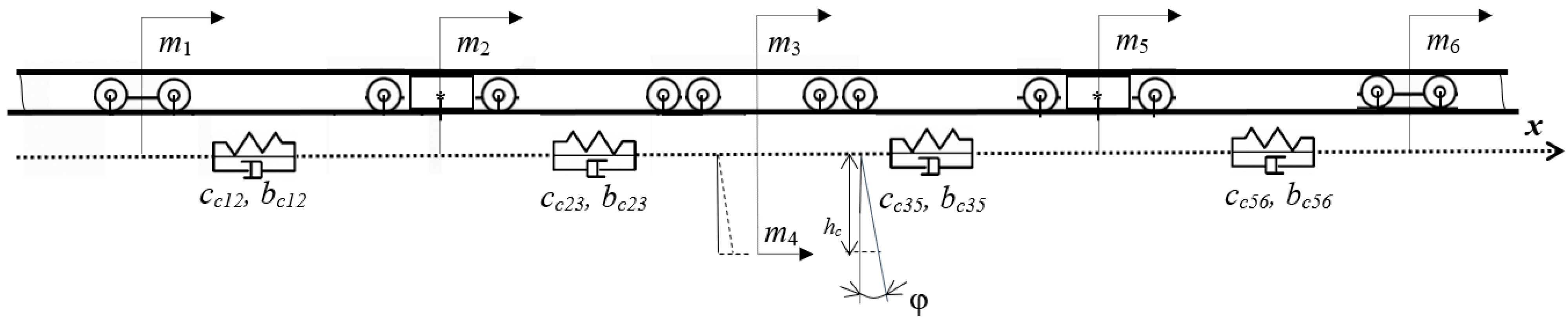
The arrangement of the suspended monorail system affects the longitudinal oscillations of the rolling stock. Similar to [27], the case of transportation of large-sized cargo along a monorail is considered, for example, a section of mechanized support weighing up to 32 tons. The layout of the rolling stock for this case is shown in Figure 2 [27].

Considering Figure 2, the studies from [27] and the properties of the non-integer integro-differential apparatus, a fractional differential mathematical model is obtained that describes the motion of a system of longitudinal oscillations of a large-sized cargo transported along a suspended monorail road. The mathematical model describing this process can be written as follows:

$$m_1{}^{GL}D^{\gamma }{x}_1+T_{q1}\left(t\right)+c_{c12}\left(x_1-x_2\right)+b_{c12}{}^{C}D^{\alpha }\left(x_1-x_2\right)=0,$$

(28)

$$\begin{array}{l}{m}_2{}^{GL}D^{\gamma }{x}_2+F_{q2}\left(t\right)-c_{c12}\left(x_1-x_2\right)-b_{c12}{}^{C}D^{\alpha }\left(x_1-x_2\right)+\\ +c_{c23}\left(x_2-x_3\right)+b_{c23}{}^{C}D^{\alpha }\left(x_2-x_3\right)=0,\end{array}$$

(29)

$$\begin{array}{l}{m}_3{}^{GL}D^{\gamma }{x}_3-c_{c23}\left(x_2-x_3\right)-b_{c23}{}^{C}D^{\alpha }\left(x_2-x_3\right)+\\ +c_{c35}\left(x_3-x_5\right)+b_{c35}{}^{C}D^{\alpha }\left(x_3-x_5\right)+{\displaystyle \frac{m_{4}g}{h_c}}\left(x_3-x_4\right)=0,\end{array}$$

(30)

$${}^{GL}D^{\gamma }{x}_4-{\displaystyle \frac{g}{h_c}}\left(x_3-x_4\right)=0,$$

(31)

$$\begin{array}{l}{m}_5{}^{GL}D^{\gamma }{x}_5-c_{c35}\left(x_3-x_5\right)-b_{c35}{}^{C}D^{\alpha }\left(x_3-x_5\right)+\\ +c_{c56}\left(x_5-x_6\right)+b_{c56}{}^{C}D^{\alpha }\left(x_5-x_6\right)+F_{q5}\left(t\right)=0,\end{array}$$

(32)

$$m_6{}^{GL}D^{\gamma }{x}_6-c_{c56}\left(x_5-x_6\right)-b_{c56}{}^{C}D^{\alpha }\left(x_5-x_6\right)+T_{q6}\left(t\right)=0.$$

(33)

A matrix representation of the model (28)–(33), analogous to Equation (17), is obtained. The mass, stiffness, and damping matrices are square with dimension 6.

For the mathematical model (28)–(33), the values of the corresponding matrices and vectors will be as follows:

$$\begin{gathered} f\left(t\right)=\left[\begin{array}{ccccccccc}{T}_{q1}\left(t\right)& F_{q2}\left(t\right)& 0& 0& 0& 0& 0& F_{q5}\left(t\right)& T_{q6}\left(t\right)\end{array}\right], \\ M={\left[\begin{array}{cccccc}{m}_1& m_2& m_3& 1& m_5& m_6\end{array}\right]}^T,\overline{X\left(t\right)}={\left[\begin{array}{cccccc}{x}_1& x_2& x_3& x_4& x_5& x_6\end{array}\right]}^T, \\ \overline{X^{\left(\gamma \right)}\left(t\right)}={\left[\begin{array}{cccccc}{x}_1^{\left(\gamma \right)}& x_2^{\left(\gamma \right)}& x_3^{\left(\gamma \right)}& x_4^{\left(\gamma \right)}& x_5^{\left(\gamma \right)}& x_6^{\left(\gamma \right)}\end{array}\right]}^T, \\ \overline{X^{\left(\alpha \right)}\left(t\right)}={\left[\begin{array}{cccccc}{x}_1^{\left(\alpha \right)}& x_2^{\left(\alpha \right)}& x_3^{\left(\alpha \right)}& x_4^{\left(\alpha \right)}& x_5^{\left(\alpha \right)}& x_6^{\left(\alpha \right)}\end{array}\right]}^T, \\ K=\left(\begin{array}{cccccc}{c}_{c12}& -c_{c12}& 0& 0& 0& 0\\ -c_{c12}& \left(c_{c12}+c_{c23}\right)& -c_{c23}& 0& 0& 0\\ 0& -c_{c23}& \left(c_{c23}+c_{c35}+{\displaystyle \frac{m_{4}g}{h_c}}\right)& -{\displaystyle \frac{m_{4}g}{h_c}}& -c_{c35}& 0\\ 0& 0& -{\displaystyle \frac{g}{h_c}}& {\displaystyle \frac{g}{h_c}}& 0& 0\\ 0& 0& -c_{c35}& 0& \left(c_{c35}+c_{c56}\right)& -c_{c56}\\ 0& 0& 0& 0& -c_{c56}& c_{c56}\end{array}\right), \\ C=\left(\begin{array}{cccccc}{b}_{c12}& -b_{c12}& 0& 0& 0& 0\\ -b_{c12}& \left(b_{c12}+b_{c23}\right)& -b_{c23}& 0& 0& 0\\ 0& -b_{c23}& \left(b_{c23}+b_{c35}\right)& 0& -b_{c35}& 0\\ 0& 0& 0& 0& 0& 0\\ 0& 0& -b_{c35}& 0& \left(b_{c35}+b_{c56}\right)& -b_{c56}\\ 0& 0& 0& 0& -b_{c56}& b_{c56}\end{array}\right). \end{gathered}$$

The algorithm for numerical implementation of the mathematical model (28)–(33) will be similar to that described above for the fractional differential mathematical model which describes the motion the longitudinal oscillation system of the rolling stock at the moment of braking (8)–(16). Only the matrix and vectors will be different, which will have dimensions 6 × 6 and 6, respectively. Therefore, they will take the following form:

$$\begin{gathered} A=\left(\begin{array}{cccccc}{a}_{11}& a_{12}& 0& 0& 0& 0\\ a_{21}& a_{22}& a_{23}& 0& 0& 0\\ 0& a_{32}& a_{33}& a_{34}& a_{35}& 0\\ 0& 0& a_{43}& a_{44}& 0& 0\\ 0& 0& a_{53}& 0& a_{55}& a_{56}\\ 0& 0& 0& 0& a_{65}& a_{66}\end{array}\right),B=\left(\begin{array}{c}{b}_1\\ b_2\\ b_3\\ b_4\\ b_5\\ b_6\end{array}\right),X=\left(\begin{array}{c}{x}_1^m\\ x_2^m\\ x_3^m\\ x_4^m\\ x_5^m\\ x_6^m\end{array}\right), \\ {a}_{11}={\displaystyle \frac{m_1}{h^{\gamma }}}+c_{c12}+{\displaystyle \frac{b_{c12}}{h^{\alpha }\mathsf{\Gamma }\left(2-\alpha \right)}},a_{12}=a_{21}=-c_{c12}-{\displaystyle \frac{b_{c12}}{h^{\alpha }\mathsf{\Gamma }\left(2-\alpha \right)}},a_{23}=-{\displaystyle \frac{b_{c23}}{h^{\alpha }\mathsf{\Gamma }\left(2-\alpha \right)}}, \\ {a}_{22}={\displaystyle \frac{m_2}{h^{\gamma }}}+c_{c12}+c_{c23}+{\displaystyle \frac{1}{h^{\alpha }\mathsf{\Gamma }\left(2-\alpha \right)}}\left(b_{c12}+b_{c23}\right),a_{32}=-c_{c23}-{\displaystyle \frac{b_{c23}}{h^{\alpha }\mathsf{\Gamma }\left(2-\alpha \right)}}, \\ {a}_{33}={\displaystyle \frac{m_3}{h^{\gamma }}}+{\displaystyle \frac{m_{4}g}{h_c}}+c_{c23}+c_{c35}+{\displaystyle \frac{1}{h^{\alpha }\mathsf{\Gamma }\left(2-\alpha \right)}}\left(b_{c23}+b_{c35}\right),a_{34}=-{\displaystyle \frac{m_{4}g}{h_c}},a_{35}=-c_{c35}-{\displaystyle \frac{b_{c35}}{h^{\alpha }\mathsf{\Gamma }\left(2-\alpha \right)}},a_{43}=-{\displaystyle \frac{g}{h_c}}, \\ {a}_{44}={\displaystyle \frac{m_4}{h^{\gamma }}}+{\displaystyle \frac{g}{h_c}},a_{53}=-c_{c35}-{\displaystyle \frac{b_{c35}}{h^{\alpha }\mathsf{\Gamma }\left(2-\alpha \right)}}, \\ {a}_{55}={\displaystyle \frac{m_5}{h^{\gamma }}}+c_{c35}+c_{c56}+{\displaystyle \frac{1}{h^{\alpha }\mathsf{\Gamma }\left(2-\alpha \right)}}\left(b_{c35}+b_{c56}\right),a_{56}=-c_{c56}-{\displaystyle \frac{b_{c56}}{h^{\alpha }\mathsf{\Gamma }\left(2-\alpha \right)}}, \\ {a}_{66}={\displaystyle \frac{m_6}{h^{\gamma }}}+c_{c56}+{\displaystyle \frac{b_{c56}}{h^{\alpha }\mathsf{\Gamma }\left(2-\alpha \right)}},a_{65}=-c_{c56}+{\displaystyle \frac{b_{c56}}{h^{\alpha }\mathsf{\Gamma }\left(2-\alpha \right)}}, \\ {b}_1=-{\displaystyle \frac{b_{c12}}{h^{\alpha }\mathsf{\Gamma }\left(2-\alpha \right)}}{\displaystyle {\displaystyle \sum _{k=1}^m}{w}_k\left(x_1^{m-k}-x_2^{m-k}\right)}-{\displaystyle \frac{m_1}{h^{\gamma }}}{\displaystyle {\displaystyle \sum _{k=1}^m}{q}_k{x}_1^{m-k}}-T_{q1}, \\ {b}_2={\displaystyle \frac{b_{c12}}{h^{\alpha }\mathsf{\Gamma }\left(2-\alpha \right)}}{\displaystyle {\displaystyle \sum _{k=1}^m}{w}_k\left(x_1^{m-k}-x_2^{m-k}\right)}-{\displaystyle \frac{b_{c23}}{h^{\alpha }\mathsf{\Gamma }\left(2-\alpha \right)}}{\displaystyle {\displaystyle \sum _{k=1}^m}{w}_k\left(x_2^{m-k}-x_3^{m-k}\right)-\frac{m_2}{h^{\gamma }}{\displaystyle \sum _{k=1}^m{q}_k{x}_2^{m-k}}-F_{q2}}, \\ {b}_3={\displaystyle \frac{b_{c23}}{h^{\alpha }\mathsf{\Gamma }\left(2-\alpha \right)}}{\displaystyle {\displaystyle \sum _{k=1}^m}{w}_k\left(x_2^{m-k}-x_3^{m-k}\right)}-{\displaystyle \frac{b_{c35}}{h^{\alpha }\mathsf{\Gamma }\left(2-\alpha \right)}}{\displaystyle {\displaystyle \sum _{k=1}^m}{w}_k\left(x_3^{m-k}-x_5^{m-k}\right)-\frac{m_3}{h^{\gamma }}{\displaystyle \sum _{k=1}^m{q}_k{x}_3^{m-k}}}, \\ {b}_4=-{\displaystyle \frac{1}{h^{\gamma }}}{\displaystyle \sum _{k=1}^m{q}_k{x}_4^{m-k}},b_5={\displaystyle \frac{b_{c35}}{h^{\alpha }\mathsf{\Gamma }\left(2-\alpha \right)}}{\displaystyle {\displaystyle \sum _{k=1}^m}{w}_k\left(x_3^{m-k}-x_5^{m-k}\right)}-{\displaystyle \frac{b_{c56}}{h^{\alpha }\mathsf{\Gamma }\left(2-\alpha \right)}}{\displaystyle {\displaystyle \sum _{k=1}^m}{w}_k\left(x_5^{m-k}-x_6^{m-k}\right)-\frac{m_5}{h^{\gamma }}{\displaystyle \sum _{k=1}^m{q}_k{x}_5^{m-k}-F_{q5}}}, \\ {b}_6={\displaystyle \frac{b_{c56}}{h^{\alpha }\mathsf{\Gamma }\left(2-\alpha \right)}}{\displaystyle {\displaystyle \sum _{k=1}^m}{w}_k\left(x_5^{m-k}-x_6^{m-k}\right)-}{\displaystyle \frac{m_6}{h^{\gamma }}}{\displaystyle {\displaystyle \sum _{k=1}^m}{q}_k{x}_6^{m-k}}-T_{q6}. \end{gathered}$$

3. Results and Discussion

Software Implementation. For the numerical implementation of the fractal mathematical models (8)–(16) and (28)–(33), software in the Python 3.11 programming language was developed.

The parameters used in the numerical simulations were selected to represent a physically realistic operating regime of the suspended monorail system, consistent with typical values reported in the literature on rail dynamics and vibration analysis. When direct experimental identification was not available, the parameters were chosen within commonly accepted engineering ranges to ensure physically meaningful system behavior.

The primary objective of this study was not parameter identification or calibration for a specific experimental setup, but the investigation of the influence of fractional-order dynamics on the qualitative and quantitative behavior of the system. Therefore, the selected parameters serve as reference values for comparative analysis of integer- and fractional-order models.

In this context, it is further emphasized that all parameter values are fully consistent with the baseline model [39], ensuring methodological coherence and enabling a fair comparison between the proposed fractional formulation and the classical integer-order framework.

Model 1

The analysis of the results of modeling the longitudinal movements ($x_1,\dots ,x_9$) of a suspended monorail road with consideration of different orders of fractional differentiation is shown in Figure 1. Graphical dependences are plotted for the following parameters: $m_1=m_6=m_9=0.2t$; $m_2=2.0t;$ $m_3=m_5=m_8=8.0t;$ $m_4=1.0t$; $m_7=1.0t$; $h_c=1m$; $c_c=800\mathrm{k}\mathrm{N}/\mathrm{m}$; $b_c=5\mathrm{k}\mathrm{N}·\mathrm{s}/\mathrm{m}$ and the initial speed of the rolling stock, which is equal to 4 m/s, $F_q\left(t\right),T_{q1}\left(t\right),T_{q9}\left(t\right)$ = 30 kN.

Figure 3, Figure 4, Figure 5 and Figure 6 present the simulation results of suspended monorail displacements obtained for various orders of fractional differentiation (${\mathrm{x}}_1,...,{\mathrm{x}}_9$).

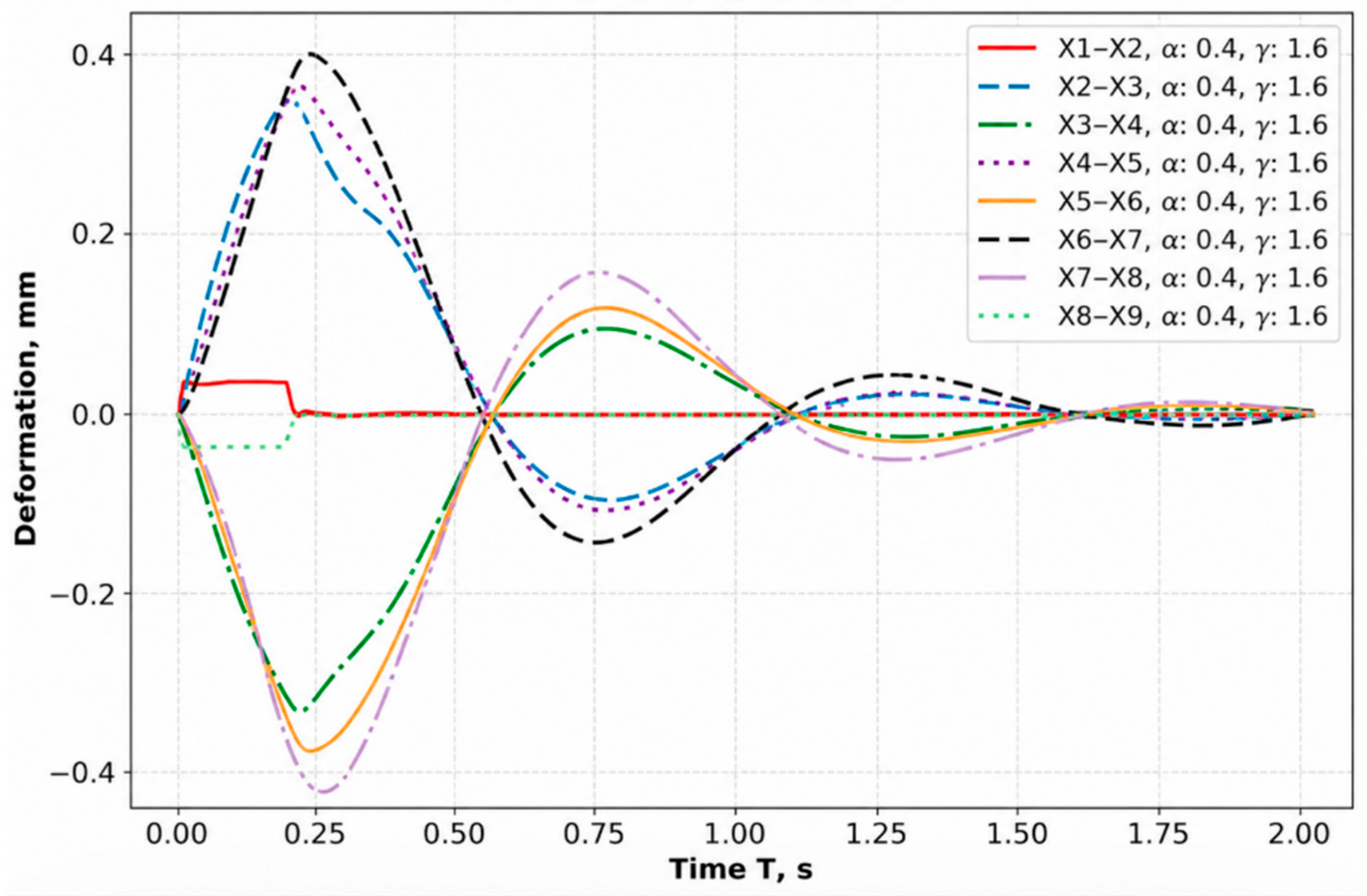
The diagram in Figure 3 shows the dependence of displacements (${\mathrm{x}}_1,...,{\mathrm{x}}_9$) on time for the following parameters: α = 0.4, γ = 1.6. The use of different orders of fractional derivatives allows memory effects and non-local interactions within the material and the structure to be accounted for. This is evident in the graphs—nodes closer to the source of disturbance exhibit more abrupt changes, whereas distant nodes respond with a delay and smaller amplitudes. For all nodes in the system, the displacement amplitudes initially reach a maximum rapidly and then gradually decay. This behavior corresponds to the expected physical response of a damped suspended structure. A phase discrepancy is observed between different nodes, reflecting the propagation of the oscillatory wave along the monorail system. Unlike traditional models, which only consider local effects and linear interactions, fractional models enable the simulation of anomalous diffusion processes and system “memory,” making the results more physically meaningful and realistic. These findings are consistent with the results reported in [4,10,12], which emphasized the effectiveness of fractional models in predicting deformation–relaxation processes and material dynamics.

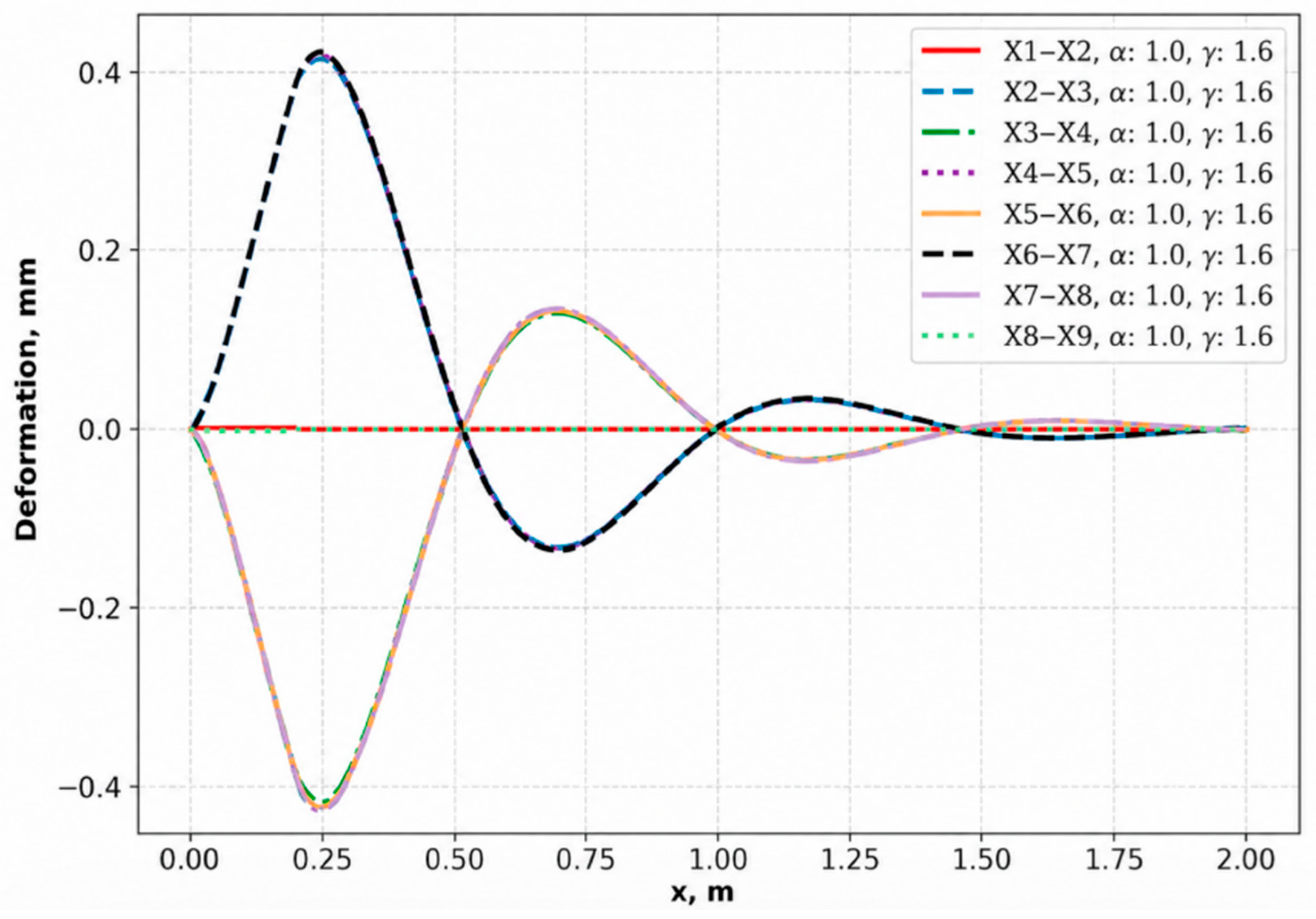
Both diagrams (Figure 4) depict the change in longitudinal displacements (x_1,…,x_9) at a fixed coefficient γ = 1.6, but with different values of α = 0.4, α = 1.0. The natural shape of the graphs and the appropriate damping of oscillations indicate that the developed numerical algorithm in Python reliably reproduces the dynamics of the suspended monorail system. This provides the possibility of using the model for structural optimization and vibration level prediction, which is crucial for enhancing the reliability and safety of operation.

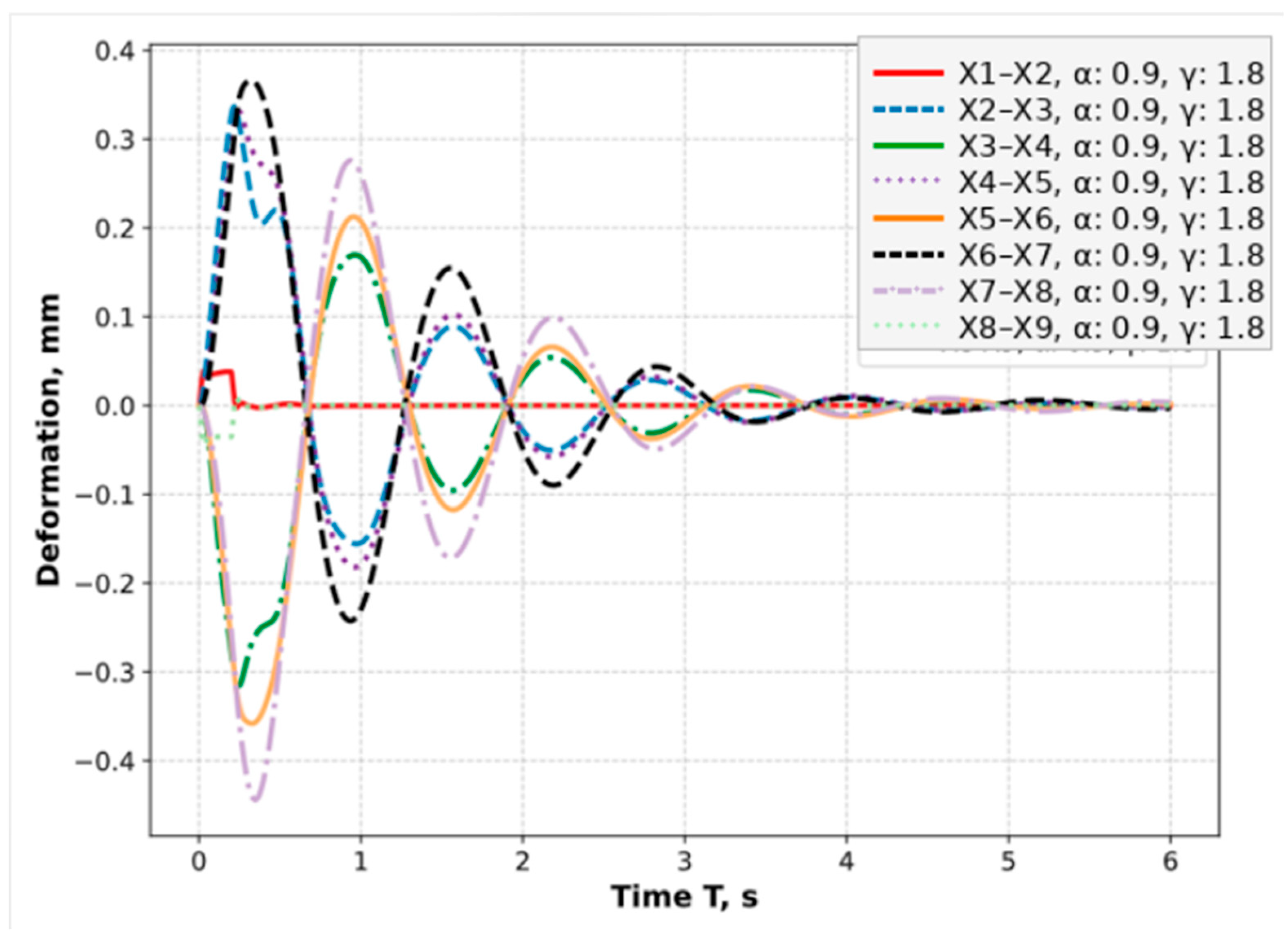
Figure 5 characterizes the change in longitudinal displacements ($x_1,...,x_9$) for α = 0.9 and γ = 1.8 The amplitudes of oscillations are noticeably lower, especially for the X1–X4 magnitudes. This indicates the effective damping of oscillations in the initial sections of the track. Such behavior may suggest the presence of differentiated damping in the system, provided not only by classical friction mechanisms but also by material “memory” effects, which are modeled using fractional derivatives.

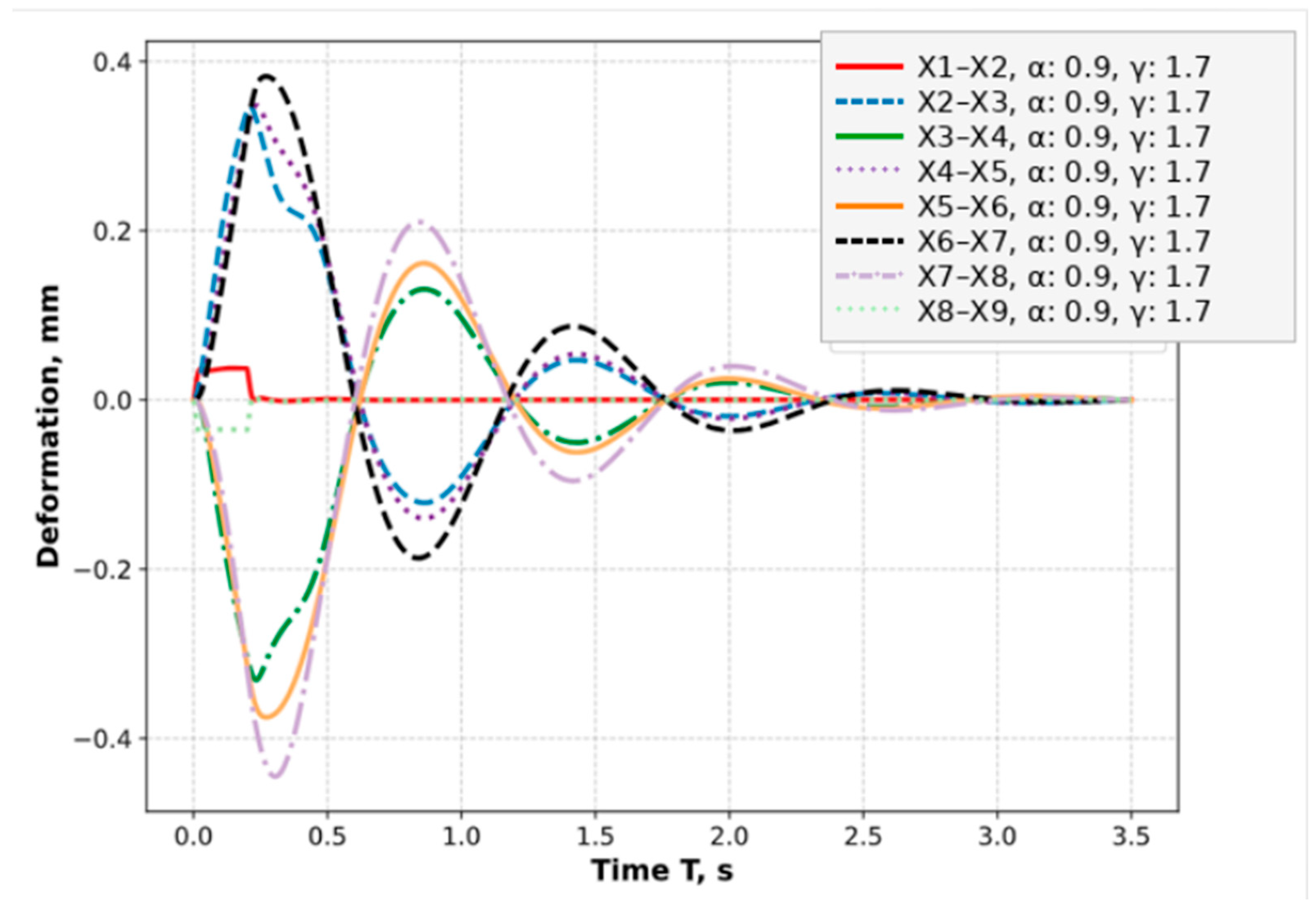
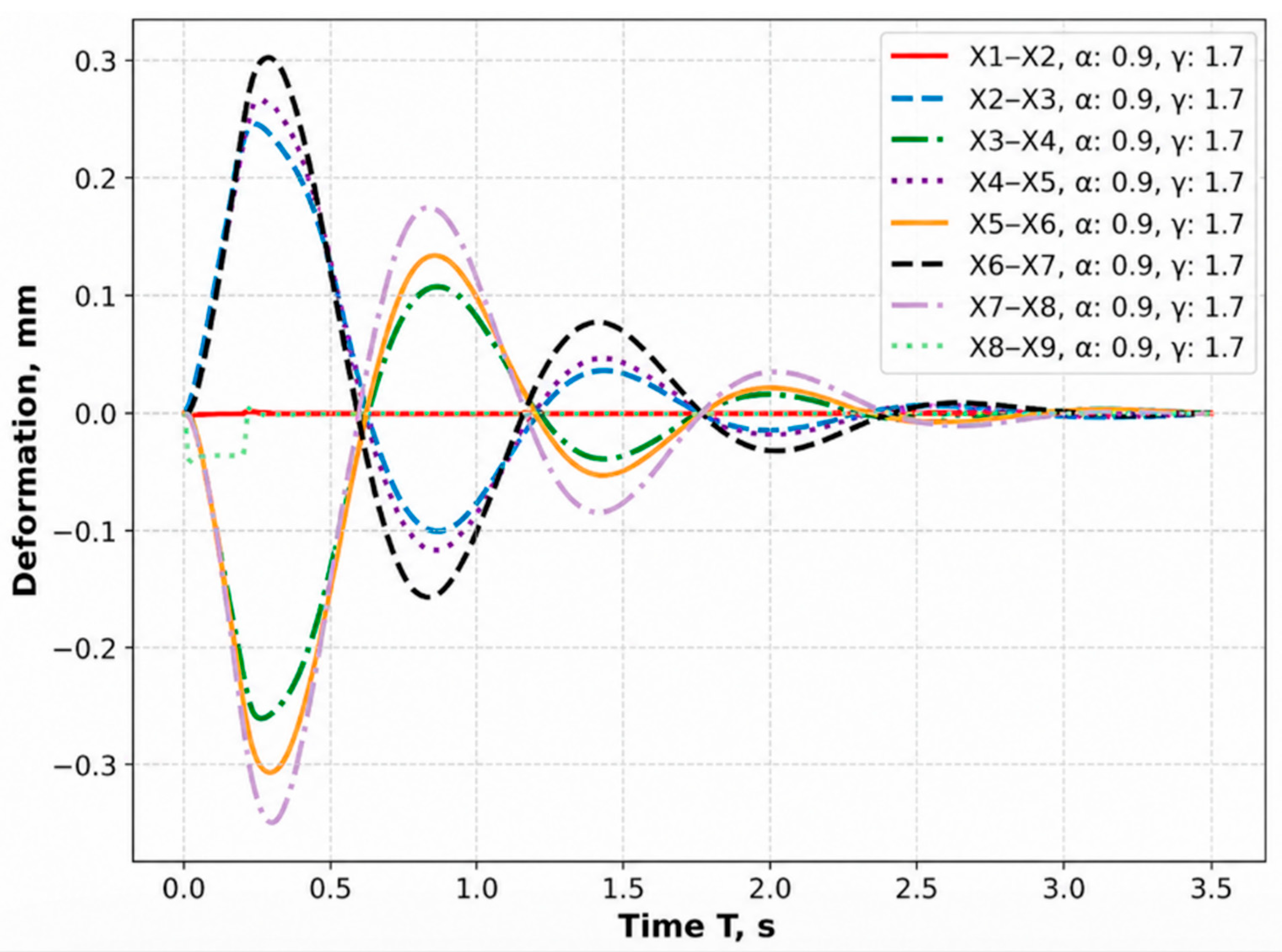
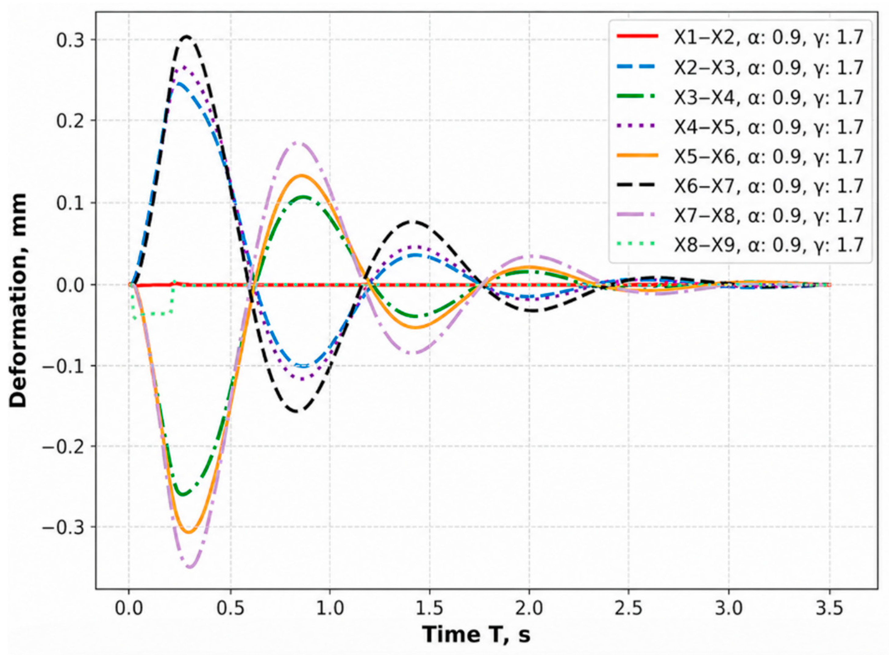
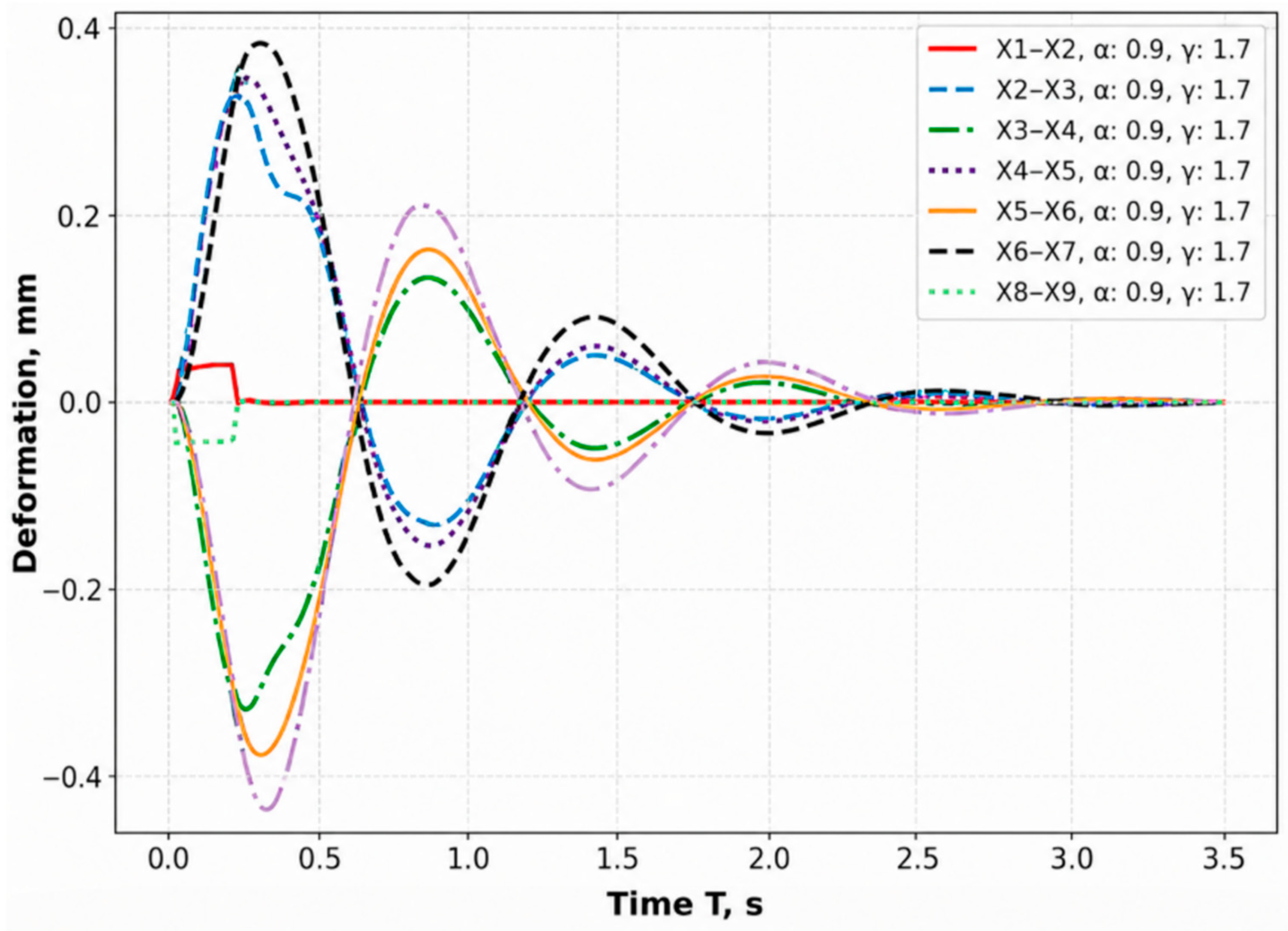
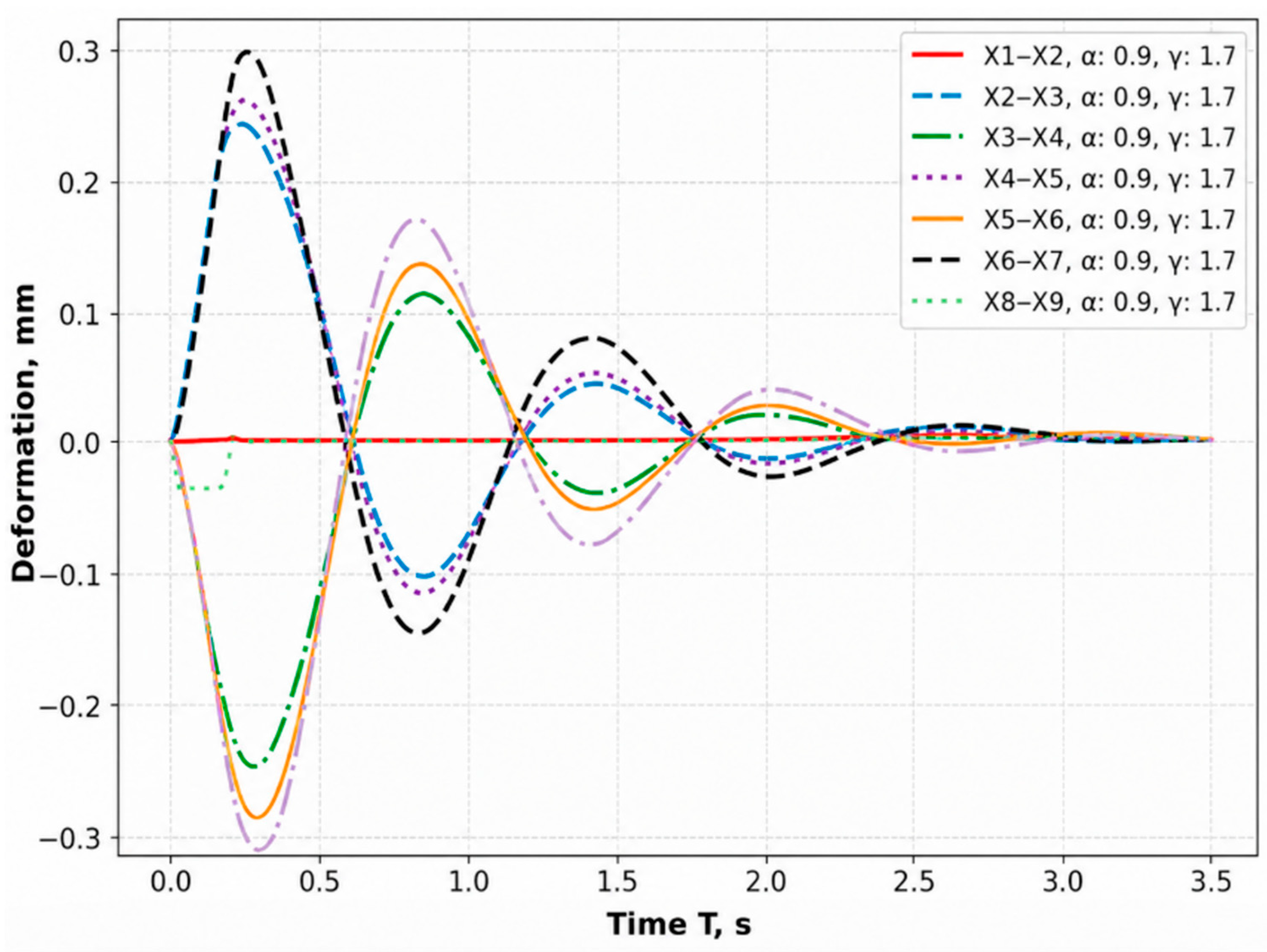
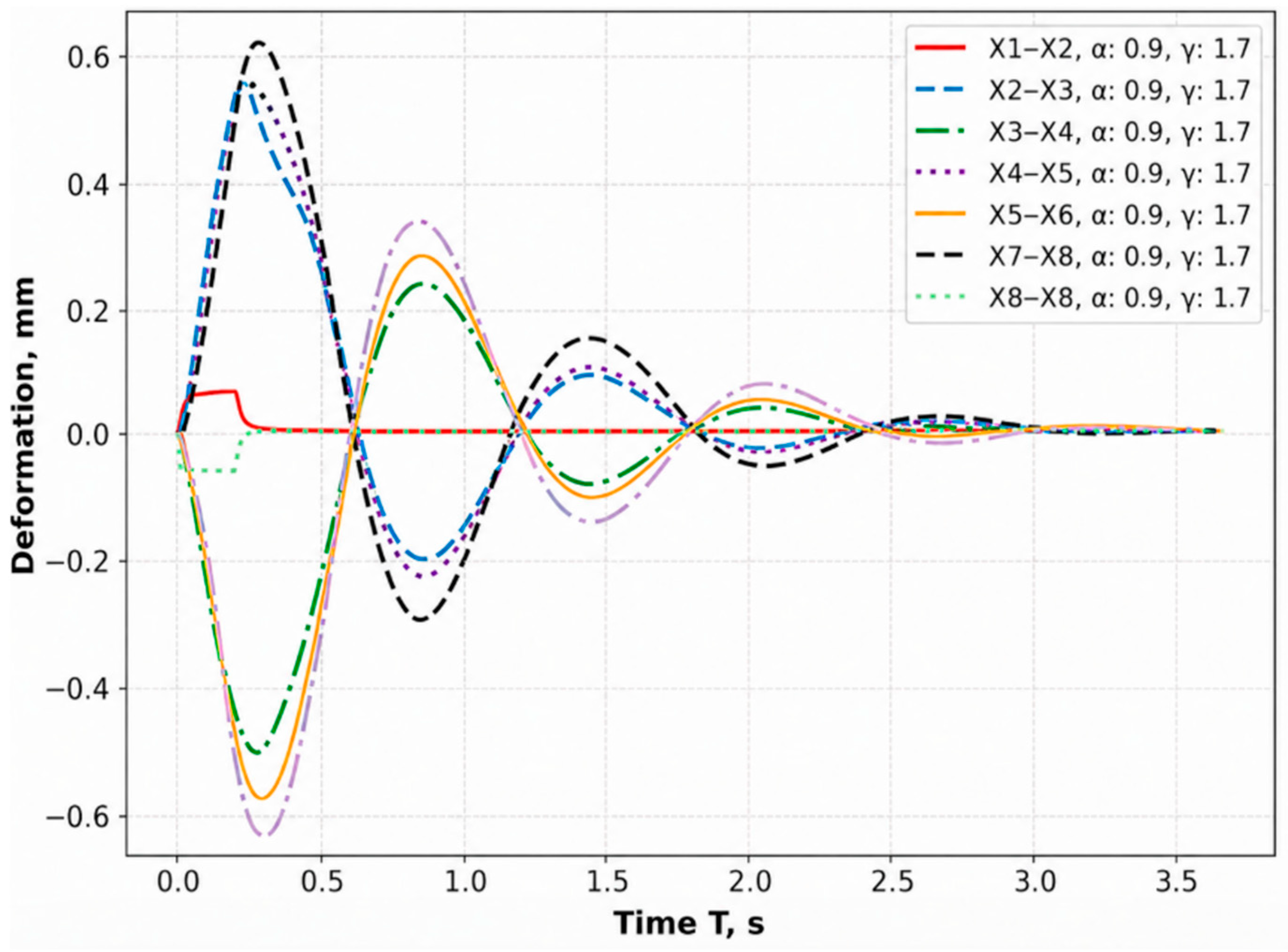
The conducted analysis showed that the order of fractional differentiation α affects the dynamic behavior of the suspended monorail system, primarily influencing the amplitude of oscillations and the rate of their decay (Figure 6, Figure 7, Figure 8, Figure 9, Figure 10 and Figure 11). A decrease in the value of α leads to more pronounced oscillations and slower damping, whereas higher values of the parameter result in more intensive energy dissipation and faster stabilization. At the same time, it was established that when transitioning to integer-order derivatives, the results of the fractional differential model are in good agreement with those obtained within the classical approach [40], which confirms the correctness of the developed model and its consistency with the known solutions.

At the same time, a comparison of the obtained graphs for different loading scenarios and connection coefficients indicates that the qualitative pattern of the process remains similar: in all cases, damped oscillations with comparable phase characteristics are observed. Quantitative differences are mainly manifested in changes to the maximum amplitudes and minor temporal shifts.

Figure 7 presents the simulation results of suspended monorail displacements considering variations in braking forces for different orders of fractional differentiation ($F_q\left(t\right),T_{q1}\left(t\right),T_{q9}\left(t\right)$ = (30, 0, 30)).

Figure 8, Figure 9 and Figure 10 present the simulation results of suspended monorail displacements considering variations variations in stiffness and damping coefficients for different orders of fractional differentiation.

${\mathrm{c}}_{\mathrm{c}12},{\mathrm{c}}_{\mathrm{c}24},{\mathrm{c}}_{\mathrm{c}46},{\mathrm{b}}_{\mathrm{c}12},{\mathrm{b}}_{\mathrm{c}24},{\mathrm{b}}_{\mathrm{c}46}$ = (800, 800, 800, 10, 10, 10)—stiffness coefficients and damping coefficients of the couplings, respectively.

The stiffness and damping coefficients of the couplings are given as: $c_{c12},c_{c24},c_{c46},b_{c12},b_{c24},b_{c46}$ = (900, 900, 900, 20, 20, 20).

Model 2

Figure 11 presents the simulation results of suspended monorail displacements considering various orders of fractional differentiation (${\mathrm{x}}_1,...,{\mathrm{x}}_9$).

The results are consistent with each other and closely align with other numerical estimates, confirming the correctness of the developed model and its stability with respect to parameter variations. This suggests that the fractional approach adequately describes the system dynamics and can be employed for further research and practical calculations, particularly in modeling complex dissipative processes in transport structures.

For the quantitative assessment of discrepancies between the results obtained from the fractional differential model of the dynamic behavior of the suspended monorail system, a statistical criterion based on the correlation coefficient was used. This approach allows the evaluation of the degree of agreement between solutions obtained under different model formulations and the corresponding reference (classical) results, as well as the quantitative characterization of the influence of the fractional order on the variation of the system’s dynamic response.

This criterion is defined as follows:

$$\Delta ={\displaystyle \frac{\left|{\rho }_{\epsilon \overline{\epsilon }}\right|}{\sqrt{1-{\rho }_{\epsilon \overline{\epsilon }}^2}}}\sqrt{n-2}$$

(34)

where $n$ is the number of points used for comparison of the quantities. ${\rho }_{\epsilon \overline{\epsilon }}$ is the correlation coefficient, defined by the following relation:

$${\rho }_{\epsilon \overline{\epsilon }}={\displaystyle \frac{{\displaystyle \sum _{i=0}^n\left({\epsilon }_i-{\epsilon }_{avg}\right)\left({\overline{\epsilon }}_i-{\overline{\epsilon }}_{avg}\right)}}{\sqrt{{\displaystyle \sum _{i=0}^n{\left({\epsilon }_i-{\epsilon }_{avg}\right)}^2{\displaystyle \sum _{i-0}^n{\left({\overline{\epsilon }}_i-{\overline{\epsilon }}_{avg}\right)}^2}}}}}$$

(35)

where ${\epsilon }_i,{\overline{\epsilon }}_i$—denotes the deformation values corresponding to each model according to the derived expressions and represents the experimental data,

$${\epsilon }_{avg}={\displaystyle \frac{1}{n+1}}{\displaystyle \sum _{i=0}^n{\epsilon }_i},{\overline{\epsilon }}_{avg}={\displaystyle \frac{1}{n+1}}{\displaystyle \sum _{i=0}^n{\overline{\epsilon }}_i}.$$

Considering Formulas (34) for the criterion Δ and (35) for the correlation coefficient, a quantitative assessment of the agreement between the numerical simulation results and the experimental data reported in [39] was performed. The obtained values of the correlation coefficient lie within the range $\rho =0.92\text{–}0.98$, while the corresponding values of the criterion are within $\mathsf{\Delta }=15\text{–}35$, indicating a high level of agreement. These values of Δ significantly exceed the commonly accepted threshold (Δ > 10), confirming the adequacy of the developed model and the reliability of the obtained results. Thus, the results of the numerical experiment are in good agreement with the experimental data presented in [39], which confirms the effectiveness of applying fractional calculus to the modeling of the dynamics of suspended transport systems.

In addition, the reliability of the obtained results was further supported by both theoretical consistency and practical validation, including agreement with known analytical solutions, as well as consistency with previously published studies and observed physical behavior of the system.

4. Conclusions

As a result of this study, a fractal model of longitudinal oscillations of large cargo on a suspended monorail system was developed and validated, utilizing fractional differential operators in the sense of Caputo and Grünwald–Letnikov. The model accounts for nonlinear interactions, memory effects, and anomalous diffusion processes that occur under real operating conditions.

Fractional calculus was used as a mathematical tool to model the dynamical effects induced by multiscale surface irregularities, rather than to perform a direct fractal analysis of the system. The use of fractional derivatives of different orders allows for the capture of non-local interactions and structural “memory” effects, making the simulations more physically meaningful. Analysis of the displacement graphs showed that nodes closer to the disturbance source respond more abruptly, while distant nodes exhibit delays and smaller oscillation amplitudes.

The developed numerical algorithm implemented in Python accurately reproduces system dynamics, ensures proper damping of oscillations, and enables identification of moments when the system approaches critical states (e.g., overload or loss of stability).

The model demonstrates high accuracy in predicting oscillatory processes, allowing for the following:

• forecasting the wear of rails and rolling stock components;
• assessing the stability of motion and overall system reliability;
• optimizing the design of the suspended monorail systems considering their nonlinear behavior.

The practical significance of this work lies in its application to design, diagnostics, and operational maintenance of monorail systems, enhancing reliability and safety. Specifically, the use of the fractal model enables more precise vibration control and more efficient energy management, which can ultimately enable, for example, higher operational speeds without compromising performance.

The scientific novelty of this study lies in the integration of multiscale surface irregularity effects within a fractional differential modeling framework, providing a powerful tool for describing complex transport phenomena characterized by memory and spatial nonlocality, which cannot be adequately captured by classical integer-order models.