Adaptive B-Spline-Based Distortion Modeling and Calibration for Cameras with Freeform Lenses

Abstract

Freeform lenses introduce spatially varying and asymmetric distortions that cannot be reliably modeled by conventional calibration frameworks. This work presents a calibration approach that represents the distortion field using a bicubic B-spline surface and integrates it directly into parameter estimation. To address instability caused by uneven sampling, an adaptive knot placement strategy guided by distortion-aware density estimation is introduced, together with a regularized control-point formulation. These components enable stable optimization under non-uniform and sparse observations. Experiments on synthetic and real datasets show that the proposed method consistently achieves sub-pixel reprojection accuracy (0.39–0.80 pixels on synthetic data and 0.24 pixels on real data) and improves geometric rectification quality compared with representative parametric and non-parametric approaches. The results indicate that continuous distortion modeling with adaptive spatial parameterization provides a reliable solution for calibrating complex lens systems.

1. Introduction

Freeform optical components are widely used in modern imaging and display systems due to their flexible surface design [1,2,3]. Compared with traditional rotationally symmetric lenses, freeform lenses simplify optical system structures and improve image quality but introduce more complex distortions [4]. These distortions are often asymmetric and spatially varying. As a result, they do not satisfy the central projection and radial symmetry assumptions of conventional calibration models. This makes freeform lens calibration an important problem.

Freeform surface measurement methods are relatively mature [5,6], but they focus on surface shape and alignment, not imaging calibration. In terms of imaging modeling, freeform optical systems have a non-rotationally symmetric structure. They often exhibit significant spatially varying and asymmetric distortion, which challenges traditional calibration methods. Existing camera calibration methods fall into three categories: parametric, non-parametric, and deep learning-based.

Parametric methods, such as Zhang’s method [7] and the Kannala–Brandt fisheye model [8], rely on the central projection assumption and use low-order polynomials to model distortion. Various extensions have been proposed to improve flexibility. Real-Moreno et al. [9] relax the global symmetry assumption and reduce local errors via quadrant-wise fitting, but boundary continuity and generalization remain limited. Recent works [10,11] incorporate geometric constraints such as line preservation, yet their effectiveness is limited in texture-sparse or curve-dominated scenes. Rameau et al. [12] focus on multi-camera system optimization but stay within conventional distortion modeling. Lochman et al. [13] offer strong generality and robust initialization through a back-projection model, but their performance on non-central distortions from freeform surfaces still needs validation. Overall, these methods still depend on central projection and weak symmetry assumptions. When distortion is strongly spatially varying and non-axisymmetric, their modeling capability is often insufficient, leading to unstable calibration.

Non-parametric methods model distortion as dense or continuous mappings. For example, digital image correlation (DIC)-based methods [14,15] estimate pixel-wise displacement fields accurately but rely on DIC reference images and complex procedures. TPS spline-based models [16] and moving least squares (MLS) methods [17] offer flexible continuous distortion representation. Researchers have reduced the impact of uneven sampling through uniform sampling and minimum curvature estimation [18] and have introduced weighted least squares with feature uncertainty to suppress overfitting in low-quality regions [19]. These approaches improve local robustness, but their performance remains highly dependent on sampling distribution and local feature quality. Consequently, they struggle to ensure global continuity and consistency in regions with severe distortion variation or sparse constraints. Moreover, most non-parametric methods use a decoupled strategy, handling distortion correction and camera estimation separately. This separation often causes geometric inconsistency between distortion modeling and camera estimation, reducing overall stability and accuracy.

Deep learning-based methods use data-driven neural networks for camera parameter estimation or distortion correction. Parameter regression methods [20,21,22] rely on predefined camera models and cannot represent complex asymmetric distortions well. Reconstruction-based techniques [23,24,25] can handle asymmetric distortions and show some potential for freeform lenses, but they require extensive data collection. Although existing studies emphasize generalization, their evaluations are mostly based on traditional distortion types. Furthermore, works such as [26,27,28,29] focus mainly on radial distortion modeling and correction, while [30,31,32] target the rolling shutter effect in CMOS sensors. These methods handle highly nonlinear and complex distortions effectively, but their performance heavily depends on training data distribution. At the same time, they typically optimize for visual quality rather than geometric accuracy. Thus, they lack explicit geometric constraints and physical interpretability, which limits their use in calibration tasks that require precise parameter estimation.

Spline-based methods offer unique advantages. Compared to MLS and TPS, B-splines better balance local control and global consistency. They are gradually gaining attention, and some studies have extended them to specific scenarios. Kawanishi et al. [33] use B-splines to fit radial distortion for ultra-wide-angle stereo vision. Hu et al. [34] use two B-spline curves to describe underwater imaging distortion caused by refraction and the lens. However, both methods are designed for specific scenarios and have limited generalization.

Based on the above discussion, freeform lens calibration faces three major challenges. First, traditional models cannot represent asymmetric and spatially varying distortions. Second, many non-parametric methods decouple distortion modeling from camera estimation, making results highly sensitive to initialization. Third, calibration data distribution is often non-uniform, especially near image boundaries, which may cause model instability or overfitting.

To address these issues, we propose an adaptive B-spline-based calibration framework. A cubic B-spline models distortion as a continuous 2D function and integrates it directly into the calibration process. This enables joint estimation of distortion and camera parameters. An adaptive knot placement strategy and control point regularization enhance stability under non-uniform sampling. The Levenberg–Marquardt (LM) method then jointly optimizes all parameters, reducing sensitivity to initialization and improving calibration accuracy.

The main contributions of this work are summarized as follows:

• Unified B-spline calibration formulation: A continuous bicubic B-spline distortion field is incorporated into the camera projection model. This integrates distortion estimation and camera calibration into one optimization framework, eliminating separate correction steps.
• Jacobian-guided stability analysis: We analyze the Jacobian structure of the proposed model with respect to camera parameters and control points. The analysis shows that inactive basis functions, insufficient knot-span coverage, or weak distortion derivatives cause zero Jacobian columns, rank deficiency, and unstable control-point estimation. These results clarify the observability requirements for spline-based joint calibration and justify the proposed adaptive knot generation strategy.
• Stability-aware adaptive knot generation: We introduce a distortion-weighted knot generation strategy using kernel density estimation (KDE). This strategy preserves basis function activation and numerical stability under non-uniform calibration point distributions. Combined with dual-constrained control-point regularization, it improves robustness against sparse data and local overfitting.
• Experimental validation: Experiments on synthetic and real-world freeform lens datasets confirm sub-pixel calibration accuracy. Reprojection errors range from 0.39 to 0.80 pixels on synthetic distortions and reach 0.24 pixels on real data. Ablation studies further validate the effectiveness of the proposed method.

2. Proposed Methods

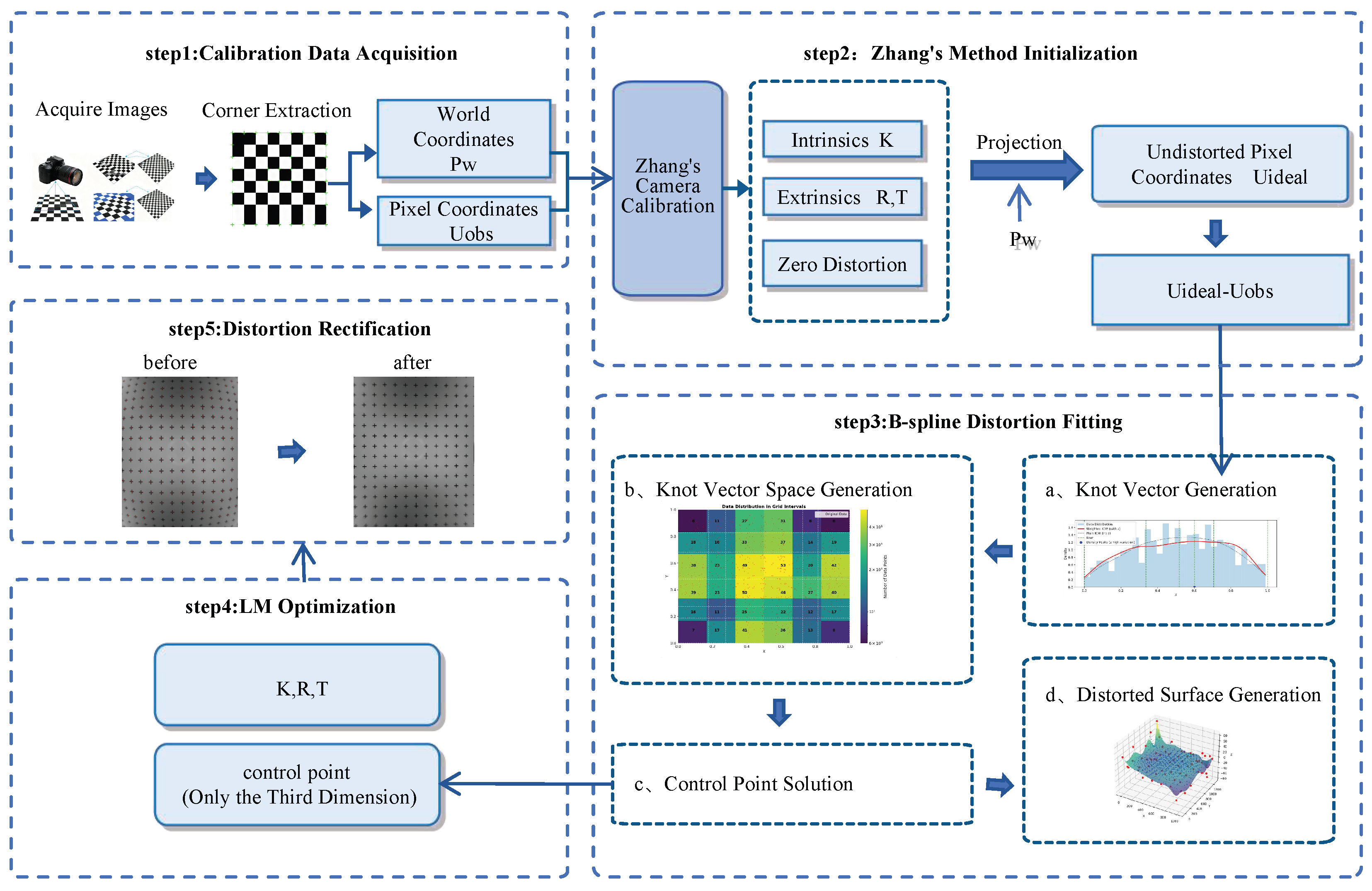
The proposed method employs bicubic B-splines to calibrate the distortion of freeform lenses, enabling joint estimation of camera intrinsic parameters, extrinsic parameters, and spatially varying distortion fields. First, a global projection model incorporating a B-spline distortion model is constructed. Subsequently, the optimization stability conditions are derived through Jacobian matrix and numerical stability analysis. Based on this, we propose an adaptive knot generation strategy driven by weighted kernel density estimation (KDE) and a control point estimation method with dual constraints combining L2 regularization and Laplacian smoothing, aiming to enhance the accuracy and robustness of the model. Finally, L-M nonlinear optimization is employed to jointly optimize all parameters. The overall workflow is illustrated in Figure 1.

The projection pipeline maps 3D world points to distorted 2D image coordinates through coordinate transformations. For clarity,

Table 1. Coordinate systems and notation.

Symbol	Quantity	Coordinate System
$P_w$	3D coordinates of a point in the world frame	World
$P_c$	3D coordinates in the camera reference frame	Camera
$X_c,Y_c,Z_c$	Components of $P_c$ along the camera axes	Camera
$x_n,y_n$	Normalized image coordinates after perspective division	Image Plane
$u_{\mathrm{ideal}},v_{\mathrm{ideal}}$	Undistorted pixel coordinates prior to distortion correction	Pixel
$u,v$	Normalized coordinates scaled to the $[0,1]\times [0,1]$ domain	Pixel-based
$\mathrm{\Delta }x,\mathrm{\Delta }y$	Lens distortion offsets in horizontal and vertical directions	Pixel-based
$u_d,v_d$	Final distorted pixel coordinates after applying distortion	Pixel
$u_{\mathrm{obs}},v_{\mathrm{obs}}$	Observed calibration image coordinates	Pixel

summarizes the symbolic representations and corresponding physical interpretations used throughout this formulation.

2.1. Global Camera Model with B-Spline Distortion

We employ Zhang’s calibration method [7] for initialization. By capturing multiple images of a planar calibration pattern from various orientations, we first estimate the initial camera parameters while neglecting lens distortion. These parameters include the intrinsic matrix K (comprising focal lengths $f_x$, $f_y$, principal point coordinates $c_x$, $c_y$, and skew coefficient s), as well as the extrinsic parameters (rotation matrix R and translation vector t) for each image.

The complete projection process, which maps a 3D world point $P_w$ to its corresponding 2D image coordinates while accounting for lens distortion, is formulated as follows. This pipeline defines the functional relationship between the estimated parameters and the final reprojection error.

The world point $P_w$ is first transformed into the camera coordinate system using the extrinsic parameters:

$$P_c=R{P}_w+t.$$

(1)

The point $P_c$ is then further projected onto the normalized image plane via standard perspective division:

$$x_n={\displaystyle \frac{X_c}{Z_c}},y_n={\displaystyle \frac{Y_c}{Z_c}}.$$

(2)

These normalized coordinates are subsequently converted into ideal (undistorted) pixel coordinates using the intrinsic camera parameters:

$$u_{\mathrm{ideal}}=f_x·x_n+c_x,v_{\mathrm{ideal}}=f_y·y_n+c_y.$$

(3)

Based on these estimated parameters, the world coordinates of the calibration pattern corners are projected to obtain their ideal pixel coordinates. The discrepancy between these coordinates and the observed pixel coordinates defines the observed distortion field:

$$\mathbf{d}=\left[\begin{array}{c}\mathrm{\Delta }x\\ \mathrm{\Delta }y\end{array}\right]=\left[\begin{array}{c}{u}_{\mathrm{obs}}-u_{\mathrm{ideal}}\\ v_{\mathrm{obs}}-v_{\mathrm{ideal}}\end{array}\right],$$

(4)

where $\mathbf{d}$ denotes the distortion vector, and $\mathrm{\Delta }x$, $\mathrm{\Delta }y$ represent the distortion offsets along the horizontal and vertical image axes, respectively.

To model this distortion field using a bicubic B-spline surface, the undistorted pixel coordinates are first normalized to the domain $[0,1]\times [0,1]$ using the image dimensions:

$$u={\displaystyle \frac{u_{\mathrm{ideal}}}{\mathrm{W}-1}},v={\displaystyle \frac{v_{\mathrm{ideal}}}{\mathrm{H}-1}},$$

(5)

where $\mathrm{W}$ and $\mathrm{H}$ represent the image width and height, respectively. This normalization establishes a unified reference frame essential for the B-spline formulation.

The lens distortion offsets at normalized image coordinates are then modeled using bicubic B-spline surfaces:

$$\begin{array}{cc}\hfill \mathrm{\Delta }x(u,v)& =\sum _{i,j}{N}_{i,p}\left(u\right)N_{j,q}\left(v\right)P_{ij}^x,\hfill \end{array}$$

(6)

$$\begin{array}{cc}\hfill \mathrm{\Delta }y(u,v)& =\sum _{i,j}{N}_{i,p}\left(u\right)N_{j,q}\left(v\right)P_{ij}^y,\hfill \end{array}$$

(7)

where $\left\{P_{ij}^x\right\}$ and $\left\{P_{ij}^y\right\}$ represent the control point grids for each distortion component; $N_{i,p}$ and $N_{j,q}$ are the p-th and q-th degree B-spline basis functions; and i, j index the control points.

The final, distorted pixel coordinates $(u_d,v_d)$ are obtained by adding the computed distortion offsets to the undistorted pixel coordinates:

$$u_d=u_{\mathrm{ideal}}+\mathrm{\Delta }x(u,v),v_d=v_{\mathrm{ideal}}+\mathrm{\Delta }y(u,v).$$

(8)

The residual vector r for a single observed image point $(u_{\mathrm{obs}},v_{\mathrm{obs}})$ is thus defined as the difference between the projected-distorted coordinates and the observation:

$$r={[u_d-u_{\mathrm{obs}},v_d-v_{\mathrm{obs}}]}^T.$$

(9)

This residual depends on all parameters involved in the pipeline: the extrinsic parameters (R, t), the intrinsic parameters ($f_x,f_y,c_x,c_y$), and the distortion parameters (the control point values $\left\{P_{ij}^x\right\},\left\{P_{ij}^y\right\}$). The primary objective of this work is to accurately model the distortion vector field $\mathbf{d}$ using this bicubic B-spline formulation.

2.2. Jacobian and Numerical Stability Analysis

In the previous section, a unified camera calibration framework is established using B-spline modeling. Since the behavior of B-spline fitting inherently depends on data distribution characteristics, integrating the distortion model into a comprehensive optimization framework and examining its numerical properties becomes necessary. Accordingly, this section analyzes the Jacobian matrix arising in the nonlinear optimization process and further investigates the essential stability conditions to guarantee convergence and well-posedness.

2.2.1. Jacobian Matrix Derivation

The Jacobian block for intrinsic parameters $[f_x,c_x,f_y,c_y]$ is:

$${\displaystyle \frac{\mathcal{\partial }r}{\mathcal{\partial }[f_x,c_x,f_y,c_y]}}=\left[\begin{array}{cccc}{\displaystyle \frac{\mathcal{\partial }{u}_d}{\mathcal{\partial }{f}_x}}& {\displaystyle \frac{\mathcal{\partial }{u}_d}{\mathcal{\partial }{c}_x}}& 0& 0\\ 0& 0& {\displaystyle \frac{\mathcal{\partial }{v}_d}{\mathcal{\partial }{f}_y}}& {\displaystyle \frac{\mathcal{\partial }{v}_d}{\mathcal{\partial }{c}_y}}\end{array}\right],$$

(10)

where ${\displaystyle \frac{\mathcal{\partial }{u}_d}{\mathcal{\partial }{f}_x}}=x_n\left(1+{\displaystyle \frac{1}{W-1}}{\displaystyle \frac{\mathcal{\partial }\mathrm{\Delta }x}{\mathcal{\partial }u}}\right)$, and ${\displaystyle \frac{\mathcal{\partial }{u}_d}{\mathcal{\partial }{c}_x}}=1+{\displaystyle \frac{1}{W-1}}{\displaystyle \frac{\mathcal{\partial }\mathrm{\Delta }x}{\mathcal{\partial }u}}$.

The stability conditions include three aspects. First, normalized coordinates must be non-zero, meaning $x_n\ne 0$ and $y_n\ne 0$. Second, distortion derivatives must satisfy the validity conditions, specifically ${\displaystyle \frac{\mathcal{\partial }\mathrm{\Delta }x}{\mathcal{\partial }u}}\ne -(W-1)$ and ${\displaystyle \frac{\mathcal{\partial }\mathrm{\Delta }y}{\mathcal{\partial }v}}\ne -(H-1)$. Finally, the data points must be well distributed to ensure the linear independence of the column vectors.

The Jacobian blocks for control points are:

$${\displaystyle \frac{\mathcal{\partial }r}{\mathcal{\partial }{P}_{ij}^x}}=\left[\begin{array}{c}{N}_{i,p}\left(u\right)N_{j,q}\left(v\right)\\ 0\end{array}\right],{\displaystyle \frac{\mathcal{\partial }r}{\mathcal{\partial }{P}_{ij}^y}}=\left[\begin{array}{c}0\\ N_{i,p}\left(u\right)N_{j,q}\left(v\right)\end{array}\right].$$

(11)

The stability conditions include four aspects. First, each control point has valid observations with $N_{i,p}\left(u\right)N_{j,q}\left(v\right)\ne 0$. Second, observations must cover the full parameter space. Third, the basis functions remain linearly independent. Fourth, reasonable density requires the spacing of the control points to match the complexity of the distortion.

The camera pose (extrinsic parameters) is represented using Lie algebra $\xi ={[{\mathit{\omega }}^T,{\mathit{\nu }}^T]}^T\in {\mathbb{R}}^6$, where $\mathit{\omega }\in {\mathbb{R}}^3$ is the rotation vector and $\mathit{\nu }\in {\mathbb{R}}^3$ is the translation vector. A 3D world point $P_w$ is transformed to the camera coordinate frame via the exponential map:

$$P_c=exp\left({\xi }^{\wedge }\right)P_w,$$

(12)

where ${\xi }^{\wedge }$ denotes wedge operator mapping the 6D vector $\xi$ to a $4\times 4$ antisymmetric matrix.

The Jacobian of the reprojection error with respect to the camera pose parameters is derived using the chain rule. Starting with the normalized image coordinates:

$$\begin{array}{cc}\hfill {\displaystyle \frac{\mathcal{\partial }{x}_n}{\mathcal{\partial }\xi }}& ={\displaystyle \frac{\mathcal{\partial }{x}_n}{\mathcal{\partial }{P}_c}}{\displaystyle \frac{\mathcal{\partial }{P}_c}{\mathcal{\partial }\xi }}=\left[\begin{array}{ccc}{\displaystyle \frac{1}{Z_c}}& 0& -{\displaystyle \frac{X_c}{Z_c^2}}\end{array}\right]\left[\begin{array}{cc}-P_c^{\wedge }& I_{3\times 3}\end{array}\right],\hfill \end{array}$$

(13)

$$\begin{array}{cc}\hfill {\displaystyle \frac{\mathcal{\partial }{y}_n}{\mathcal{\partial }\xi }}& ={\displaystyle \frac{\mathcal{\partial }{y}_n}{\mathcal{\partial }{P}_c}}{\displaystyle \frac{\mathcal{\partial }{P}_c}{\mathcal{\partial }\xi }}=\left[\begin{array}{ccc}0& {\displaystyle \frac{1}{Z_c}}& -{\displaystyle \frac{Y_c}{Z_c^2}}\end{array}\right]\left[\begin{array}{cc}-P_c^{\wedge }& I_{3\times 3}\end{array}\right],\hfill \end{array}$$

(14)

where $P_c^{\wedge }$ is the skew-symmetric matrix form of $P_c={[X_c,Y_c,Z_c]}^{\top }$:

$$P_c^{\wedge }=\left[\begin{array}{ccc}0& -Z_c& Y_c\\ Z_c& 0& -X_c\\ -Y_c& X_c& 0\end{array}\right].$$

(15)

The derivatives for undistorted pixel coordinates incorporate the focal lengths:

$$\begin{array}{cc}\hfill {\displaystyle \frac{\mathcal{\partial }{u}_{\mathrm{ideal}}}{\mathcal{\partial }\xi }}& =f_x{\displaystyle \frac{\mathcal{\partial }{x}_n}{\mathcal{\partial }\xi }},\hfill \end{array}$$

(16)

$$\begin{array}{cc}\hfill {\displaystyle \frac{\mathcal{\partial }{v}_{\mathrm{ideal}}}{\mathcal{\partial }\xi }}& =f_y{\displaystyle \frac{\mathcal{\partial }{y}_n}{\mathcal{\partial }\xi }}.\hfill \end{array}$$

(17)

The Jacobian of the reprojection error with respect to the Lie algebra parameters is:

$${\displaystyle \frac{\mathcal{\partial }r}{\mathcal{\partial }\xi }}=\left[\begin{array}{c}{A}_{11}{\displaystyle \frac{\mathcal{\partial }{u}_{\mathrm{ideal}}}{\mathcal{\partial }\xi }}+A_{12}{\displaystyle \frac{\mathcal{\partial }{v}_{\mathrm{ideal}}}{\mathcal{\partial }\xi }}\\ A_{21}{\displaystyle \frac{\mathcal{\partial }{u}_{\mathrm{ideal}}}{\mathcal{\partial }\xi }}+A_{22}{\displaystyle \frac{\mathcal{\partial }{v}_{\mathrm{ideal}}}{\mathcal{\partial }\xi }}\end{array}\right],$$

(18)

where the coefficients account for distortion effects:

$$\begin{array}{cccc}\hfill A_{11}& =1+{\displaystyle \frac{1}{W-1}}{\displaystyle \frac{\mathcal{\partial }\mathrm{\Delta }x}{\mathcal{\partial }u}},\hspace{1em}\hspace{1em}\hspace{1em}\hspace{1em}\hfill & \hfill A_{12}& ={\displaystyle \frac{1}{H-1}}{\displaystyle \frac{\mathcal{\partial }\mathrm{\Delta }x}{\mathcal{\partial }v}},\hfill \\ \hfill A_{21}& ={\displaystyle \frac{1}{W-1}}{\displaystyle \frac{\mathcal{\partial }\mathrm{\Delta }y}{\mathcal{\partial }u}},\hfill & \hfill A_{22}& =1+{\displaystyle \frac{1}{H-1}}{\displaystyle \frac{\mathcal{\partial }\mathrm{\Delta }y}{\mathcal{\partial }v}}.\hfill \end{array}$$

The stability conditions consist of the following six aspects. First, non-zero depth requires $Z_c\ne 0$ to avoid singularities in the derivatives. Second, valid image dimensions require $W\ne 1$ and $H\ne 1$ to prevent division by zero. Third, non-zero focal lengths require $f_x\ne 0$ and $f_y\ne 0$ to ensure a valid transformation. Fourth, non-degenerate points require $P_c\ne {[0,0,0]}^T$ to ensure valid coordinate transformations. Fifth, an active distortion model requires non-zero B-spline derivatives and control points. Sixth, a full-rank coupling matrix requires $det\left[\begin{array}{cc}{A}_{11}& A_{12}\\ A_{21}& A_{22}\end{array}\right]\ne 0$ to maintain invertibility.

The distortion derivatives ${\displaystyle \frac{\mathcal{\partial }\mathrm{\Delta }x}{\mathcal{\partial }u}}$ and ${\displaystyle \frac{\mathcal{\partial }\mathrm{\Delta }y}{\mathcal{\partial }v}}$ play a critical role in the Jacobian analysis. These derivatives are fundamentally governed by the control point grids $\left\{P_{ij}^x\right\}$ and $\left\{P_{ij}^y\right\}$ through the corresponding derivatives of the B-spline basis functions. Consequently, the control points emerge as the cornerstone parameters that dictate both the distortion characteristics and the numerical stability of the overall calibration framework.

2.2.2. Stability Conditions for B-Spline Modeling

As established by the Jacobian matrix analysis, preventing zero columns and maintaining full column rank requires that the data distribution ensures non-trivial B-spline distortion derivatives and control point activations. This subsection further examines the specific numerical stability conditions governing the B-spline formulation.

(1) 

Basis functions

The B-spline basis functions are piecewise polynomial functions defined over a set of non-decreasing real numbers known as the knot vector. For example, the knot vector in the u-direction is given by $\mathbf{U}=\{u_0,u_1,\dots ,u_{m+p+1}\}$. The basis function $N_{i,p}\left(u\right)$ in the u-direction is defined as follows: When $p=0$ (zeroth-degree basis function):

$$N_{i,0}\left(u\right)=\left\{\begin{array}{cc}1,\hfill & \mathrm{if}{u}_i\le u<u_{i+1}\hfill \\ 0,\hfill & \mathrm{otherwise}\hfill \end{array}\right..$$

(19)

When $p>0$ (p-th degree basis function):

$$N_{i,p}\left(u\right)={\displaystyle \frac{u-u_i}{u_{i+p}-u_i}}{N}_{i,p-1}\left(u\right)+{\displaystyle \frac{u_{i+p+1}-u}{u_{i+p+1}-u_{i+1}}}{N}_{i+1,p-1}\left(u\right),$$

(20)

where p represents the degree of the basis function, and i represents the index of the basis function. Each basis function can be expressed as a cubic polynomial in the form:

$$N_j\left(h\right)={\displaystyle \sum _{k=0}^3}{C}_k{h}^k,$$

(21)

where the coefficients $C_k$ depend on the nodal spacings $u_b-u_a$.

When the nodes are located at the boundary endpoints, the basis functions satisfy the following vanishing property at the nodes:

$$u=u_j\Rightarrow N_{j,3}\left(u\right)=0.$$

(22)

Each basis function comprises multiple rational components whose denominators contain products of non-uniform nodal spacings $u_b-u_a$. Partial derivatives demonstrate considerable non-trivial properties.

The partial derivatives of the displacement functions with respect to the parametric coordinates can be derived from Equations (6) and (7):

$$\begin{array}{cc}\hfill {\displaystyle \frac{\mathcal{\partial }\mathrm{\Delta }x}{\mathcal{\partial }u}}& =\sum _{i,j}{\displaystyle \frac{\mathcal{\partial }{N}_{i,p}\left(u\right)}{\mathcal{\partial }u}}{N}_{j,q}\left(v\right)P_{ij}^x,\hfill \end{array}$$

(23)

$$\begin{array}{cc}\hfill {\displaystyle \frac{\mathcal{\partial }\mathrm{\Delta }y}{\mathcal{\partial }v}}& =\sum _{i,j}{N}_{i,p}\left(u\right){\displaystyle \frac{\mathcal{\partial }{N}_{j,q}\left(v\right)}{\mathcal{\partial }v}}{P}_{ij}^y.\hfill \end{array}$$

(24)

These derivative expressions can be further expanded by incorporating the polynomial representation of the basis functions. For the cubic case where $p=3$ and $q=3$, we substitute the polynomial form:

$$\begin{array}{cc}\hfill {\displaystyle \frac{\mathcal{\partial }\mathrm{\Delta }x}{\mathcal{\partial }u}}& =\sum _{i,j}\left({\displaystyle \sum _{k=1}^3}k{C}_k^{\left(i\right)}{u}^{k-1}\right)\left({\displaystyle \sum _{l=0}^3}{D}_l^{\left(j\right)}{v}^l\right)P_{ij}^x,\hfill \end{array}$$

(25)

$$\begin{array}{cc}\hfill {\displaystyle \frac{\mathcal{\partial }\mathrm{\Delta }y}{\mathcal{\partial }v}}& =\sum _{i,j}\left({\displaystyle \sum _{k=0}^3}{C}_k^{\left(i\right)}{u}^k\right)\left({\displaystyle \sum _{l=1}^3}l{D}_l^{\left(j\right)}{v}^{l-1}\right)P_{ij}^y,\hfill \end{array}$$

(26)

where $C_k^{\left(i\right)}$ and $D_l^{\left(j\right)}$ are the polynomial coefficients for the basis functions $N_{i,3}\left(u\right)$ and $N_{j,3}\left(v\right)$ respectively, and the polynomial representation.

From the above formulation, it is evident that the existence and magnitude of the non-trivial B-spline distortion derivatives are governed by the properties of the basis function matrix and, more fundamentally, are immediately influenced by the data distribution.

(2) 

Matrix Representation of B-Spline Basis Functions

Assume the number of node vectors is $m+1$, denoted as $U=\{u_0,u_1,\dots ,u_m\}$. Let the order be p, and the number of control points be $s+1$. Then, the relationship $m=p+s+1$ holds. A data point is selected within each node interval, resulting in the set $Q=\{q_0,q_1,\dots ,q_{m-1}\}$, where each $q_j$ lies in the interval $[u_j,u_{j+1}]$.

Basis function matrix structure for $p=3$ with Non-Repeating End Nodes is as follows:

$$\left(\begin{array}{cccccc}{N}_0^P\left(q_0\right)& 0& 0& 0& \cdots & 0\\ N_0^P\left(q_1\right)& N_1^P\left(q_1\right)& 0& 0& \cdots & 0\\ N_0^P\left(q_2\right)& N_1^P\left(q_2\right)& N_2^P\left(q_2\right)& 0& \cdots & 0\\ N_0^P\left(q_3\right)& N_1^P\left(q_3\right)& N_2^P\left(q_3\right)& N_3^P\left(q_3\right)& \cdots & 0\\ ⋮& ⋮& ⋮& ⋮& \ddots & ⋮\\ 0& \cdots & N_{s-4}^P\left(q_{m-5}\right)& N_{s-3}^P\left(q_{m-5}\right)& \cdots & 0\\ 0& \cdots & 0& N_{s-3}^P\left(q_{m-4}\right)& \cdots & N_s^P\left(q_{m-1}\right)\\ 0& \cdots & 0& 0& \cdots & N_s^P\left(q_{m-1}\right)\\ 0& \cdots & 0& 0& \cdots & N_s^P\left(q_{m-1}\right)\end{array}\right)$$

(27)

The structure of the basis function matrix for $p=3$ with repeated end nodes is given as follows:

$$\left(\begin{array}{ccccccc}{N}_0^P\left(q_0\right)& N_1^P\left(q_0\right)& N_2^P\left(q_0\right)& N_3^P\left(q_0\right)& 0& \cdots & 0\\ 0& N_1^P\left(q_1\right)& N_2^P\left(q_1\right)& N_3^P\left(q_1\right)& N_4^P\left(q_1\right)& \cdots & 0\\ 0& 0& N_2^P\left(q_2\right)& N_3^P\left(q_2\right)& N_4^P\left(q_2\right)& \cdots & 0\\ ⋮& ⋮& \ddots & \ddots & \ddots & ⋮& ⋮\\ 0& \cdots & 0& N_{s-1}^P\left(q_{m-1}\right)& N_{s-2}^P\left(q_{m-1}\right)& \cdots & N_s^P\left(q_{m-1}\right)\end{array}\right)$$

(28)

The use of repeated end nodes enhances the control over data points near the boundaries. As shown in Equations (27) and (28), when end nodes are repeated, the first data point $q_0$ influences four control points. In contrast, with non-repeating end nodes, $q_0$ influences only one control point. If few data points are located near the boundaries, the influence of boundary data on the control points is reduced, causing the control points to be predominantly determined by interior data. This can lead to surface distortion when solving for the control points. Therefore, it is necessary to repeat the end nodes when constructing the node vector.

(3) 

Full Column Rank Condition of the Basis Function Matrix

The local support property of B-spline basis functions requires that the observation domain of each control point contains sufficient sampling points to ensure basis activation. In the proposed calibration framework, the observation matrix $\mathbf{N}$ exhibits a strictly banded structure, where each row contains only $p+1$ non-zero elements. If a knot span $[u_i,u_{i+1})$ lacks sufficient data points, a zero column will appear in $\mathbf{N}$. This breaks the banded continuity and leads to column-rank deficiency, preventing a unique numerical solution for the control points $P_{ij}$.

Notably, the use of repeated end knots (clamped knots) significantly increases the sensitivity of the system to the boundary data distribution.As shown in Equation (28), repeated knots cause the support of boundary basis functions to be highly concentrated. If the initial interval $[u_0,u_1)$ lacks a key observation $q_0$, the first column of the matrix becomes a zero vector, causing the boundary control points to become unconstrained. Unlike interior spans with smooth transitions, boundary spans carry critical geometric information that constrains the extrapolation behavior of the spline surface. Therefore, to ensure a full-rank matrix and suppress numerical oscillations, observations must fully cover the parameter space defined by the knot vector. Specifically, each knot span must contain at least one valid observation, especially in boundary regions where basis functions decay rapidly, to avoid system singularity or non-physical surface distortion.

2.3. Adaptive Knot Generation Based on Distortion-Weighted KDE

According to the analysis in the previous section, stable control-point estimation requires sufficient activation and coverage of the B-spline basis over the observation domain. In calibration with freeform lenses, however, checkerboard corners are only available at scattered and viewpoint-dependent image locations. As a result, uniformly distributed knots may create intervals with weak support or even empty tensor-product cells, which degrades the conditioning of the basis matrix and reduces estimation stability.

To address this issue, we construct the knot vectors adaptively based on the observed global corner distribution and local variations in the distortion response. Let $(u_i,v_i)\in {[0,1]}^2$ denote the normalized image coordinates of the ith corner, and let $z_i$ denote the corresponding distortion response ($\mathrm{\Delta }{x}_i$ or $\mathrm{\Delta }{y}_i$). The core idea is to construct a weight function using local variations of the discrete samples and to introduce weighted kernel density estimation to guide knot placement. The detailed algorithm is as follows.

(1) 

Discrete Estimation of the Weighting Term

For each direction $d\in \{u,v\}$, the samples are sorted according to that coordinate. Let $\{(d_{\left(1\right)},z_{\left(1\right)}),\dots ,(d_{\left(n\right)},z_{\left(n\right)})\}$ denote the reordered sequence, where $d_{\left(k\right)}$ is either $u_{\left(k\right)}$ or $v_{\left(k\right)}$. Rather than interpolating a dense distortion surface and differentiating it, we estimate local distortion variation directly from the discrete samples by a sliding-window statistic. The window size is defined as:

$$m=max\left(m_{min},2⌊{\displaystyle \frac{n\rho }{2}}⌋+1\right),$$

(29)

where $\rho \in (0,1)$ is the window ratio and $m_{min}$ is the minimum admissible window size. The odd-valued form ensures a symmetric neighborhood. For the k-th sorted sample, the local index set is:

$${\mathcal{N}}_k=\left\{j:max\left(1,k-{\displaystyle \frac{m-1}{2}}\right)\le j\le min\left(n,k+{\displaystyle \frac{m-1}{2}}\right)\right\}.$$

(30)

Local distortion variation along direction d is then given by sample standard deviation:

$$\begin{array}{cc}\hfill s_k^{\left(d\right)}& =\sqrt{{\displaystyle \frac{1}{|{\mathcal{N}}_k|}}\sum _{j\in {\mathcal{N}}_k}{\left(z_{\left(j\right)}-{\overline{z}}_k\right)}^2,}\hfill \end{array}$$

(31)

$$\begin{array}{cc}\hfill {\overline{z}}_k& ={\displaystyle \frac{1}{|{\mathcal{N}}_k|}}\sum _{j\in {\mathcal{N}}_k}{z}_{\left(j\right)}.\hfill \end{array}$$

(32)

The quantity $s_k^{\left(d\right)}$ serves as a discrete proxy for the local distortion-gradient magnitude: it becomes large when the response varies rapidly within a local neighborhood and small in smooth regions. Therefore, Equation (29) is implemented in practice by replacing the ideal continuous gradient magnitude with the above discrete local-variation estimate.

To avoid excessive dominance by a few isolated samples, the variation values are linearly normalized into a bounded interval:

$$w_k^{\left(d\right)}=\left\{\begin{array}{cc}{w}_{min}+(w_{max}-w_{min}){\displaystyle \frac{s_k^{\left(d\right)}-s_{min}^{\left(d\right)}}{s_{max}^{\left(d\right)}-s_{min}^{\left(d\right)}}},\hfill & s_{max}^{\left(d\right)}>s_{min}^{\left(d\right)}\hfill \\ 1,\hfill & s_{max}^{\left(d\right)}=s_{min}^{\left(d\right)}\hfill \end{array}\right.,$$

(33)

where $s_{min}^{\left(d\right)}={min}_k{s}_k^{\left(d\right)}$ and $s_{max}^{\left(d\right)}={max}_k{s}_k^{\left(d\right)}$.

We set $w_{min}=0.5$ and $w_{max}=1.5$. This range is chosen to balance model adaptability and structural stability. Specifically, the upper limit allows regions with complex distortion to increase their local knot density by up to 50% to capture fine details, while the lower limit ensures that smooth regions retain at least half of the baseline density. This lower bound prevents the grid from becoming overly sparse, which could lead to rank deficiency during the optimization process. Consequently, this strategy adaptively allocates knots based on the degree of distortion while guaranteeing the numerical robustness of the global optimization.

(2) 

Weighted KDE along the Two Image Directions

Given the directional weights, one-dimensional weighted KDE is performed separately along the u- and v-axes:

$$\begin{array}{cc}\hfill {\widehat{f}}_u\left(u\right)& ={\displaystyle \sum _{i=1}^n}{\tilde{w}}_i^{\left(u\right)}{\displaystyle \frac{1}{h_u}}K\left({\displaystyle \frac{u-u_i}{h_u}}\right),\hfill \end{array}$$

(34)

$$\begin{array}{cc}\hfill {\widehat{f}}_v\left(v\right)& ={\displaystyle \sum _{i=1}^n}{\tilde{w}}_i^{\left(v\right)}{\displaystyle \frac{1}{h_v}}K\left({\displaystyle \frac{v-v_i}{h_v}}\right),\hfill \end{array}$$

(35)

where $K(·)$ is the Gaussian kernel and

$${\tilde{w}}_i^{\left(d\right)}={\displaystyle \frac{w_i^{\left(d\right)}}{{\sum }_{j=1}^n{w}_j^{\left(d\right)}}},$$

(36)

where ${\tilde{w}}_i^{\left(d\right)}$ denotes the normalized weight in direction d.

The bandwidth along each direction $d\in \{u,v\}$ is selected by Scott’s rule under weighted sampling:

$$h_d={\widehat{\sigma }}_d{n}_{\mathrm{eff}}^{-1/5},$$

(37)

where ${\widehat{\sigma }}_d$ is the standard deviation of the samples along direction d. The effective sample size $n_{\mathrm{eff}}$ is given by

$$n_{\mathrm{eff}}={\displaystyle \frac{{\left({\sum }_{i=1}^n{w}_i^{\left(d\right)}\right)}^2}{{\sum }_{i=1}^n{\left(w_i^{\left(d\right)}\right)}^2}}.$$

(38)

This formulation preserves the standard Scott scaling while accounting for unequal sample influence. In practice, it provides a stable compromise between oversmoothing and spurious local oscillations.

(3) 

Adaptive Knot Generation and Grid Optimization

To balance model compactness and fitting accuracy, we propose a three-stage knot placement strategy based on the evaluated weighted KDE curves: initial knot generation, 1D interval merging, and 2D coverage optimization.

First, candidate knots are initialized from three sources: the normalized domain boundaries (0 and 1); the local maxima of ${\widehat{f}}_u$ and ${\widehat{f}}_v$ (to capture dense informative samples); and the empirical quartiles (25%, 50%, and 75%) to ensure global spatial coverage. These candidates are then deduplicated and sorted to form the initial 1D knot vectors.

Second, support-aware interval merging is applied to satisfy the full-rank requirement for control point estimation. For a knot vector ${\mathcal{T}}^{\left(d\right)}=\{t_0^{\left(d\right)},t_1^{\left(d\right)},\dots ,t_{M_d}^{\left(d\right)}\}$ in direction $d\in \{u,v\}$, the support count $c_r^{\left(d\right)}$ of the r-th interval is defined as:

$$c_r^{\left(d\right)}=\left|\left\{i\mid t_r^{\left(d\right)}\le d_i<t_{r+1}^{\left(d\right)}\right\}\right|,$$

(39)

where the last interval includes its right endpoint, and $|·|$ denotes the set cardinality. Let $N_{min}=max(10,N_{total}/50)$ be the minimum data threshold, where $N_{total}$ is the number of valid corners. If $c_r^{\left(d\right)}<N_{min}$, an interior knot is removed to merge the interval with an adjacent one. To limit model complexity, each dimension is capped at 15 intervals. Intervals with the fewest observations are iteratively merged until these 1D constraints are satisfied, explicitly enforcing the coverage requirement analyzed in previous section.

Finally, 2D coverage optimization is performed. Even if both 1D knot vectors meet the support criteria, the resulting tensor-product grid may still contain empty 2D cells, causing inactive basis functions in the final bicubic B-spline surface. To resolve this, we compute a 2D occupancy histogram:

$$H_{ab}=\left|\left\{i\mid u_i\in [t_a^{\left(u\right)},t_{a+1}^{\left(u\right)}),v_i\in [t_b^{\left(v\right)},t_{b+1}^{\left(v\right)})\right\}\right|.$$

(40)

If empty cells ($H_{ab}=0$) exist, the algorithm identifies the dimension with the highest number of empty cells and prioritizes interval merging along that dimension. This cross-dimensional refinement iterates (up to 30 times) until all cells contain valid observation data ($\forall a,b,H_{ab}>0$). This step mathematically eliminates the rank-deficiency risk caused by local data absence, ensuring the numerical stability of the subsequent joint optimization.

2.4. Dual-Constrained Control Point Solver

Even with stable knot distributions, the solution in regions of extreme data sparsity, such as image edges, may remain ill-posed, causing oscillatory control points and distorted surfaces. To enhance robustness, we introduce a composite regularization term.

The loss function is defined as:

$$L={\parallel \mathbf{B}\mathbf{P}-\mathbf{d}\parallel }^2+{\lambda }_1{\parallel \mathbf{P}\parallel }^2+{\lambda }_2{\parallel \mathbf{L}\mathbf{P}\parallel }^2,$$

(41)

where ${\parallel \mathbf{B}\mathbf{P}-\mathbf{d}\parallel }^2$ is the data fidelity term, ${\lambda }_1{\parallel \mathbf{P}\parallel }^2$ is an L2 regularization term that penalizes large control point values, and ${\lambda }_2{\parallel \mathbf{L}\mathbf{P}\parallel }^2$ is a smoothness constraint where $\mathbf{L}$ is a Laplacian matrix that penalizes second-order derivatives of the control point grid. The hyperparameters ${\lambda }_1$ and ${\lambda }_2$ balance fitting accuracy, numerical stability, and smoothness.

The design matrix $\mathbf{B}$ is constructed from B-spline basis functions evaluated at the parameter locations $(\mathbf{u},\mathbf{v})$. The resulting regularized system is solved via least squares:

$$\left({\mathbf{B}}^{\top }\mathbf{B}+{\lambda }_1\mathbf{I}+{\lambda }_2({\mathbf{D}}_r^{\top }{\mathbf{D}}_r+{\mathbf{D}}_c^{\top }{\mathbf{D}}_c)\right)\mathbf{P}={\mathbf{B}}^{\top }\mathbf{d},$$

(42)

where ${\mathbf{D}}_r$ and ${\mathbf{D}}_c$ are finite-difference operators along the rows and columns of the control point grid, respectively.

2.5. Full Parameter Joint Optimization

Using the initial intrinsic and extrinsic parameters along with the B-spline control points obtained from the previous steps as initial values, we construct a complete camera model to perform a final overall optimization. The Levenberg-Marquardt algorithm is employed to minimize the sum of reprojection errors over all points, where regularization terms are introduced to enhance numerical stability and ensure smoothness of the distortion surfaces. A joint bundle adjustment is carried out over all parameters:

$$\underset{K,(R_k,t_k),P}{min}{\displaystyle \sum _{k=1}^M}{\displaystyle \sum _{j=1}^N}{∥{\mathbf{u}}_{\mathrm{obs},k_j}-\pi \left(K,R_k,t_k,P,{\mathbf{u}}_j\right)∥}^2,$$

(43)

where $\pi$ denotes the projection function that incorporates the B-spline distortion model, and ${\mathbf{u}}_j$ represents the world coordinates of the corner points. This step effectively eliminates errors from the initial parameter estimates, enabling the intrinsic parameters, extrinsic parameters, and distortion model to converge to a globally optimal solution, thereby maximizing calibration accuracy.

3. Experiment Results and Analysis

To evaluate the performance of the proposed calibration framework, this paper conducts a series of experiments using both synthetic and real-world data, systematically validating the core research contributions. The experimental design primarily includes validating the framework’s accuracy under controllable distortion patterns using synthetic data, evaluating its practical application performance in industrial lens scenarios through real-world experiments, and conducting comprehensive ablation studies to analyze the individual contributions of each innovative module.

3.1. Experimental Setup

(1)

Baseline Methods and Settings

We compare the proposed method with several representative calibration methods. For a fair comparison, all methods use the same detected corners and the same 3D board coordinates. For baseline methods that need hyperparameters, we tune them individually via grid search to minimize the average reprojection error on the calibration datasets. This gives competitive and stable baseline performance. All experiments run on a desktop with an Intel Core i7-12700K CPU and 32 GB RAM. Both simulated and real datasets contain 10 calibration views. The compared methods and their settings are:

• Zhang [7]: A classic method using a global symmetric polynomial distortion model. We use the OpenCV implementation with three radial coefficients $(k_1,k_2,k_3)$ and two tangential coefficients $(p_1,p_2)$.
• BabelCalib [13]: A general framework based on central camera back-projection and hierarchical initialization. We configure it with a 9th-order Kannala–Brandt angular polynomial. This improves its ability to approximate complex nonlinear distortions, even though the model remains axis-symmetric.
• McCalib [12]: A multi-camera toolbox using co-visibility graph optimization and global bundle adjustment. It uses an 8-parameter rational polynomial model with six radial coefficients $(k_1,\dots ,k_6)$ and two tangential coefficients $(p_1,p_2)$. The co-visibility graph needs at least three common corners between two views. The maximum number of BA iterations is 500.
• MLS [17]: A non-parametric method based on moving least squares interpolation. After Zhang-based initialization, it fits the residual distortion field using a first-order local polynomial. We use a Gaussian weight $w\left(d\right)=exp(-d^2/{\sigma }^2)$. The support radius $\sigma$ is tuned via grid search over $\{5\%,10\%,15\%,20\%\}$ of the image diagonal, and the best value ($10\%$) is used. To avoid unstable extrapolation in sparse regions, we discard samples beyond $3\sigma$.
• TPS [16]: A non-parametric method based on thin-plate spline interpolation. After Zhang-based initialization, it fits two independent TPS surfaces to model the residual distortion. It uses the biharmonic kernel $\varphi \left(r\right)=r^{2}logr$. The smoothing coefficient is tuned via grid search over $\{{10}^{-6},{10}^{-5},{10}^{-4},{10}^{-3},{10}^{-2}\}$, and the best value ${10}^{-4}$ is used. To reduce boundary extrapolation instability, we use only the detected corners as sparse control points.

(2)

Implementation of the Proposed Method

We implement the proposed framework in Python 3.8 using OpenCV and SciPy. It follows the calibration pipeline described in Section 2.

Table 2. Main implementation parameters of the proposed method.

Parameter	Value	Description
B-spline order	3	Bicubic B-spline surface
Max number of knot intervals	15	Prevents over-parameterization
Min support threshold	$max(10,N_{\mathrm{total}}/50)$	Ensures active basis functions
KDE bandwidth	$\mathrm{Scott}\times 1.0$	From bandwidth ablation study (Section 3.5.2)
${\lambda }_{reg}$	${10}^{-3}$	$L_2$ regularization, from ablation study (Section 3.5.4)
${\lambda }_{smooth}$	${10}^{-3}$	Laplacian smoothing, from ablation study (Section 3.5.4)
LM max iterations	500	For nonlinear joint optimization
Convergence tolerance	${10}^{-6}$	LM stopping criterion

lists the main parameters.

Table 3. Final knot intervals and control point grids for each dataset.

Dataset	U-Direction Intervals	V-Direction Intervals	Control Point Grid Size
Radial	8	8	$11\times 11$
Fisheye	10	9	$13\times 12$
Asymmetric	9	10	$12\times 13$
YP (real data)	7	7	$10\times 10$

shows the resulting knot intervals and control point grids for each dataset.

3.2. Experiments with Synthetic Data

3.2.1. Synthetic Dataset Construction

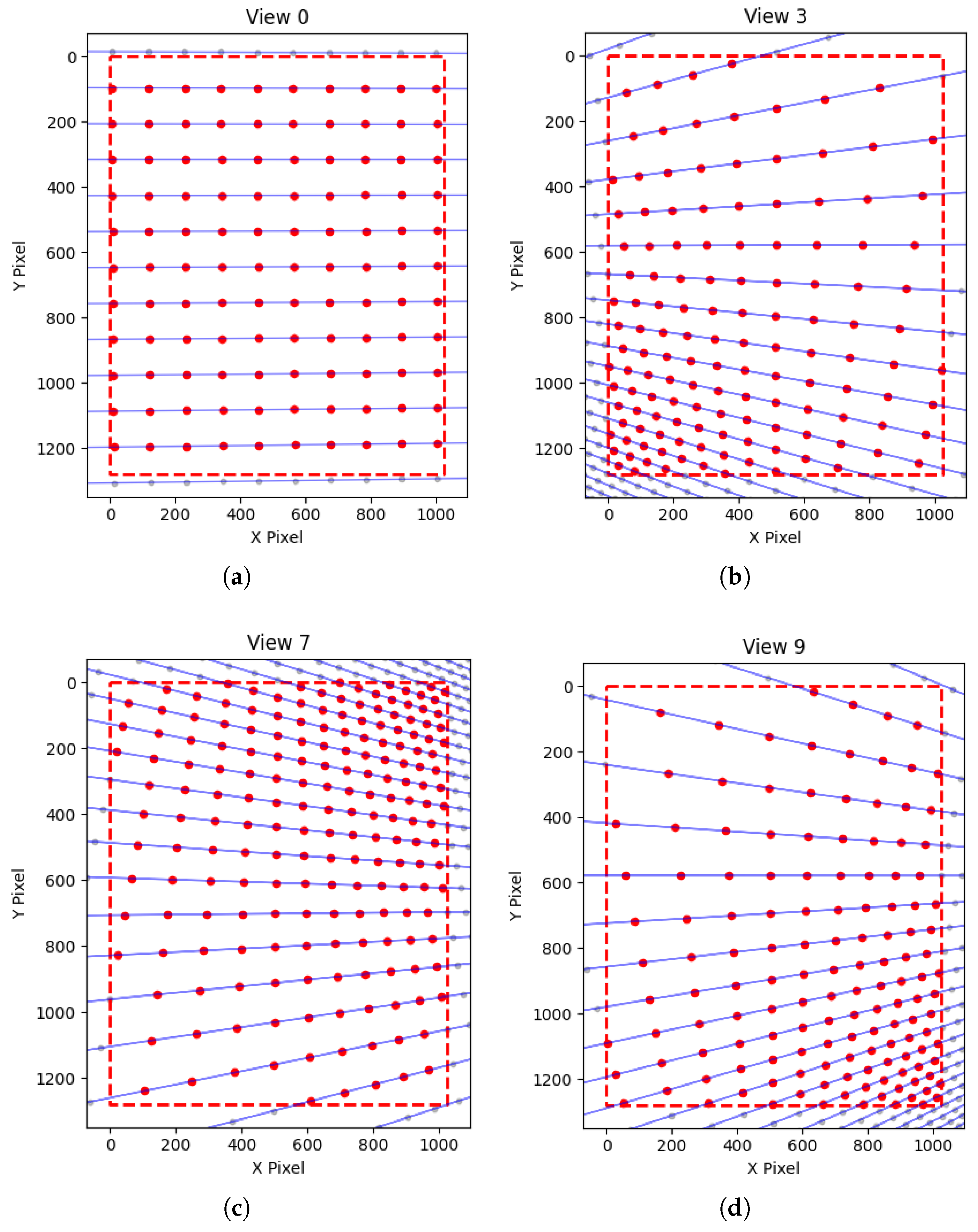
To verify the calibration accuracy, we generated simulated corner data covering the camera’s field of view (FOV). The simulated camera uses intrinsic parameters of focal length $(f_x,f_y)=(305.18,302.45)$ and a principal point of $(c_x,c_y)=(511.61,631.89)$. The extrinsic parameters were calculated from 10 different views. A $150\times 150$ checkerboard with a square size of 50.0 mm was generated at the origin of the world coordinate system. The 3D points were projected onto the image coordinates using the camera model, and points outside the valid image boundaries were filtered out. The image resolution is $1024\times 1280$, with a horizontal FOV of 118.4° and a vertical FOV of 129.4°. This process yielded a total of 1561 valid points across all views, with the number of valid points per view ranging from 108 to 215. Figure 2 illustrates the distribution of corners within the camera’s FOV for four typical views.

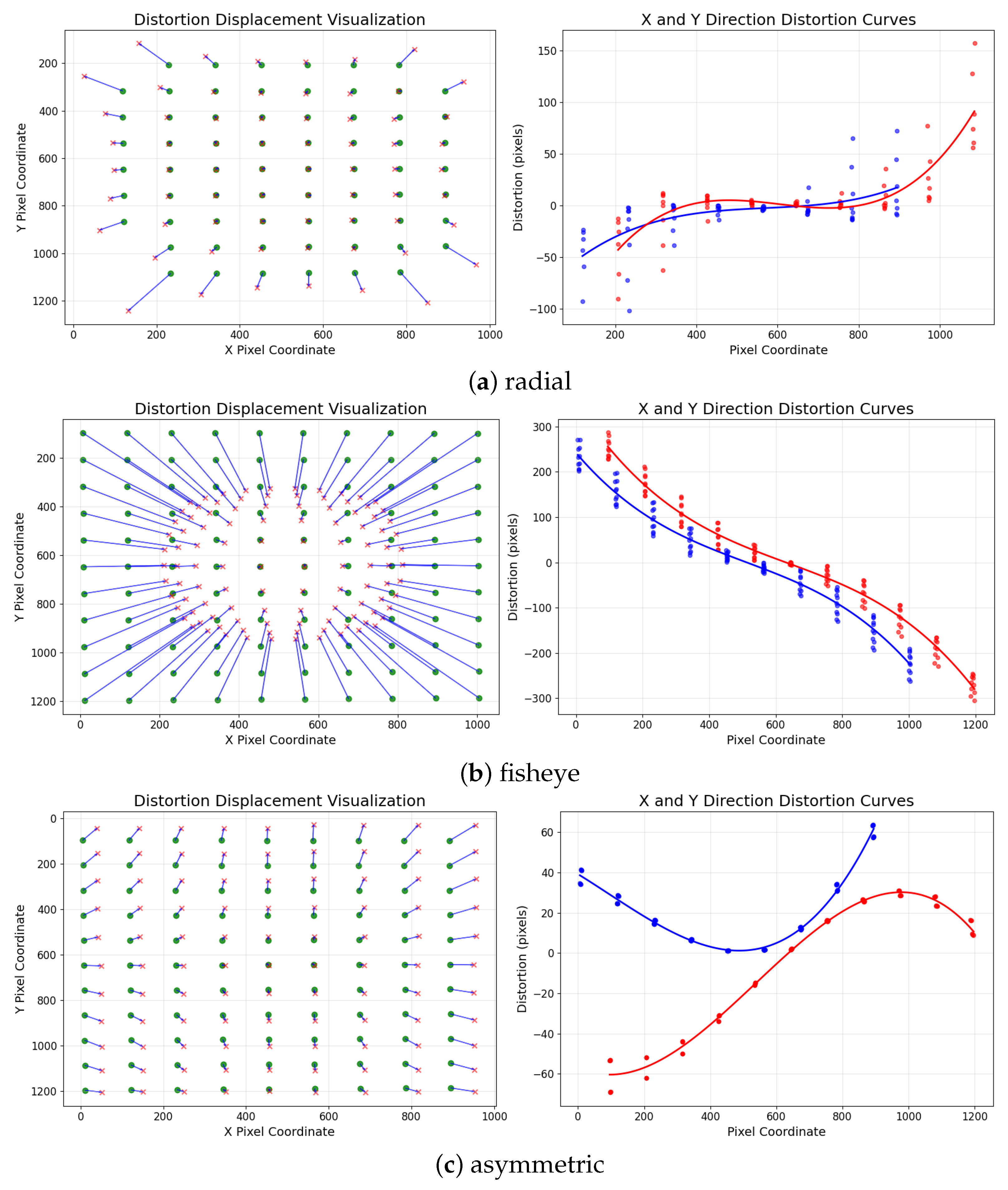
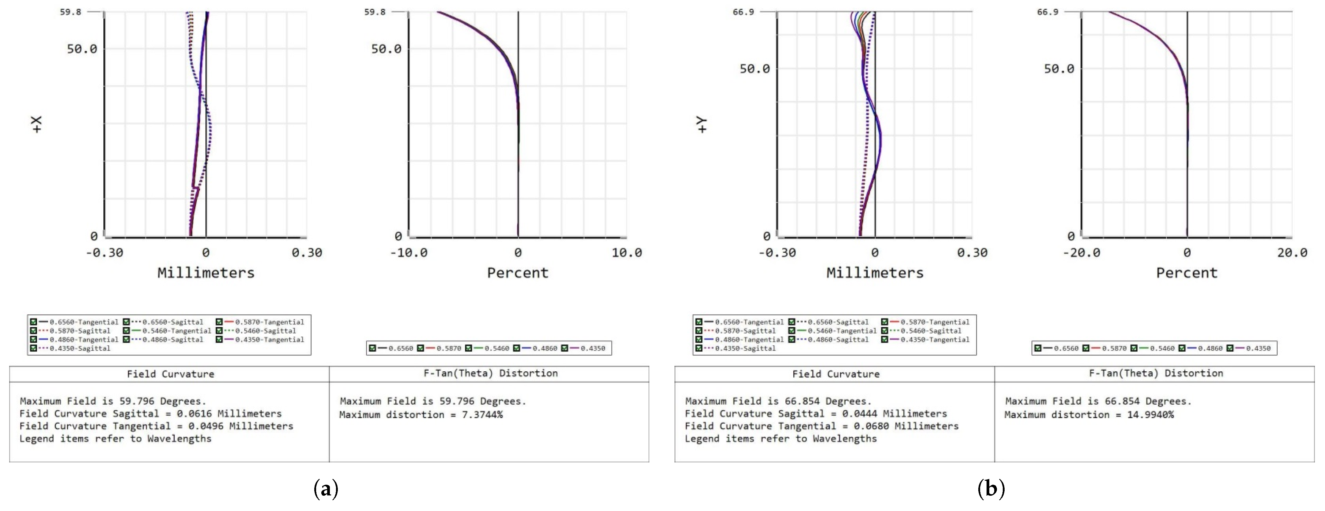
To evaluate the robustness of the proposed method, we introduced three typical types of distortion and added Gaussian noise with a mean of $\mu =0$ and a standard deviation of $\sigma =0.3$ pixels. The first type is the standard radial lens distortion, with coefficients $k_1=-0.05$, $k_2=0.0267$, $k_3=0.0067$, $p_1=0.0067$, and $p_2=-0.01$. The second type is polynomial angle-based distortion, which is a fisheye-like distortion with a strong radial component. Its coefficients are set to $k_1=-0.05$, $k_2=0.02$, $k_3=-0.01$, $k_4=0.005$, and $p_1=p_2=0.0001$. The third type is asymmetric wave distortion, a complex distortion model that combines quadrant-dependent polynomial offsets with global sinusoidal oscillations. Figure 3 shows the distortion distributions.

Both radial distortion and fisheye distortion are symmetric edge distortions. In contrast, the asymmetric distortion breaks central symmetry, resulting in significant differences between the distortion characteristics in the X and Y directions.

3.2.2. Calibration Accuracy Comparison and Analysis

Table 4. Reprojection errors across viewpoints for different distortion types (synthetic data).

Distortion Type	Method	V0	V1	V2	V3	V4	V5	V6	V7	V8	V9	Overall
radial	Zhang	2.862	3.025	3.057	3.063	2.590	2.931	3.042	3.240	3.155	2.706	3.420
	BabelCalib	1.25	1.42	1.38	1.35	1.18	1.30	1.45	1.48	1.33	1.20	1.32
	McCalib	1.20	1.35	1.38	1.28	1.15	1.22	1.38	1.42	1.28	1.18	1.284
	MLS	0.65	0.72	0.78	0.69	0.71	0.68	0.74	0.76	0.73	0.70	0.682
	TPS	0.64	0.64	0.65	0.63	0.64	0.65	0.64	0.63	0.64	0.64	0.643
	ours	0.38	0.54	0.55	0.49	0.48	0.40	0.45	0.49	0.47	0.54	0.393
asymmetric	Zhang	14.636	14.636	15.186	15.536	16.460	15.561	13.747	14.205	15.661	16.700	16.917
	BabelCalib	1.85	1.92	2.10	2.05	2.20	1.98	1.78	1.88	2.05	2.15	1.98
	McCalib	1.55	1.50	1.68	1.58	1.72	1.58	1.42	1.62	1.62	1.68	1.595
	MLS	1.25	1.18	1.32	1.21	1.29	1.24	1.27	1.30	1.26	1.23	1.255
	TPS	1.28	1.23	1.42	1.30	1.22	1.15	1.35	1.48	1.28	1.40	1.374
	ours	0.72	0.70	0.93	0.65	0.75	0.66	0.71	0.78	0.70	0.66	0.797
fisheye	Zhang	3.751	3.660	3.572	3.780	3.753	3.841	3.788	3.736	3.830	3.948	4.571
	BabelCalib	1.05	1.18	1.22	1.10	1.08	1.02	1.15	1.20	1.12	1.05	1.12
	McCalib	0.88	0.89	0.91	0.90	0.87	0.86	0.92	0.94	0.91	0.89	0.983
	MLS	0.82	0.89	0.95	0.85	0.87	0.84	0.91	0.93	0.88	0.86	0.880
	TPS	0.85	0.92	1.08	0.91	0.88	0.79	0.94	1.12	0.95	0.86	0.921
	ours	0.48	0.61	0.65	0.54	0.59	0.48	0.55	0.66	0.55	0.54	0.444

Note: Per-view values are the mean reprojection errors (MSE); Overall is the global RMSE.

shows the reprojection errors of different methods under three simulated distortion types. The proposed method achieves the best results for all distortion types, with RMSE values of 0.393, 0.444, and 0.797 pixels for radial, fisheye, and asymmetric distortions, respectively. Non-parametric methods (MLS, TPS, and ours) consistently outperform parametric ones (Zhang, BabelCalib, McCalib). This indicates that the model’s ability to represent distortion is the key factor for calibration accuracy.

For radial distortion, Zhang has an RMSE of 3.420 pixels. MLS and TPS reduce it to 0.682 and 0.643 pixels. The proposed method further reduces it to 0.393 pixels. TPS performs slightly better than MLS. This is because TPS minimizes global bending energy, which fits well with the smooth and symmetric nature of radial distortion. For fisheye distortion, Zhang increases to 4.571 pixels. MLS and TPS drop to 0.880 and 0.921 pixels. TPS is slightly worse than MLS. The global smoothness of TPS causes extrapolation errors in the highly compressed image edges, while the local support of MLS is more robust. The proposed method uses a bicubic B-spline surface with a KDE-based adaptive knot placement strategy. It achieves an RMSE of 0.444 pixels, which is about 50% and 52% better than MLS and TPS, respectively.

The largest performance gap appears under asymmetric wave distortion. Zhang fails with an RMSE of 16.917 pixels due to its radial symmetry assumption. BabelCalib and McCalib, despite their complex optimization steps, are still limited by their parametric models (e.g., Kannala–Brandt). Their errors are 1.98 and 1.595 pixels. Among non-parametric methods, MLS (1.255 pixels) is better than TPS (1.374 pixels) by about 9.5%. The local rigidity of MLS allows it to fit different image regions independently, while the global smoothness of TPS tends to smooth out local details. The proposed method achieves an RMSE of 0.797 pixels. This is 36.5% and 42.0% better than MLS and TPS. These results show the effectiveness of combining bicubic B-spline representation with adaptive knot placement and regularization.

3.2.3. Robustness Analysis Against Feature Extraction Noise

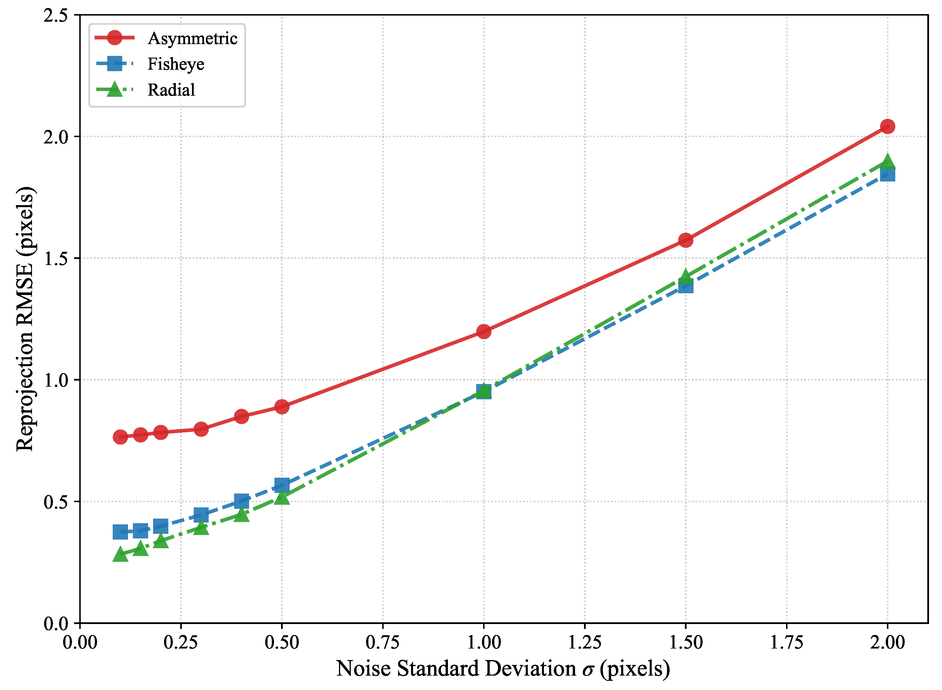
The previous experiments compared the calibration accuracy of the different methods at a fixed noise level ($\sigma =0.3$ pixels). This section further analyzes the noise robustness of the proposed method. Gaussian noise with standard deviations $\sigma$ ranging from 0.1 to 2.0 pixels was injected into the simulated corner coordinates. For the three types of distortion models, 20 independent trials were conducted at each noise level, and the average RMSE of the global reprojection error was recorded. The optimization parameters remained consistent: the regularization weight ${\lambda }_{reg}={10}^{-3}$, the smoothing constraint ${\lambda }_{smooth}={10}^{-3}$, and the convergence thresholds $ftol=xtol={10}^{-6}$.

Figure 4 and

Table 5. Noise sensitivity of the proposed method in terms of RMSE.

Distortion Type	$\mathit{\sigma }=0.1$	$0.15$	$0.2$	$0.3$	$0.4$	$0.5$	$1.0$	$1.5$	$2.0$
radial	0.283	0.307	0.339	0.393	0.447	0.518	0.956	1.424	1.899
fisheye	0.374	0.379	0.398	0.444	0.502	0.566	0.951	1.386	1.846
asymmetric	0.765	0.774	0.784	0.797	0.849	0.889	1.198	1.574	2.041

present the experimental results. The proposed method demonstrates stable performance across all distortion types: the reprojection error increases approximately linearly with the added noise, and no accuracy collapse occurs. For the asymmetric wave distortion, when the noise standard deviation increases from 0.1 to 0.3 pixels, the RMSE only rises from 0.765 to 0.797 pixels. Even under extreme noise conditions of 2.0 pixels, the global RMSE remains well constrained within 2.1 pixels.

3.3. Experiments with Real Data

3.3.1. Real-World Dataset and Experimental Setup

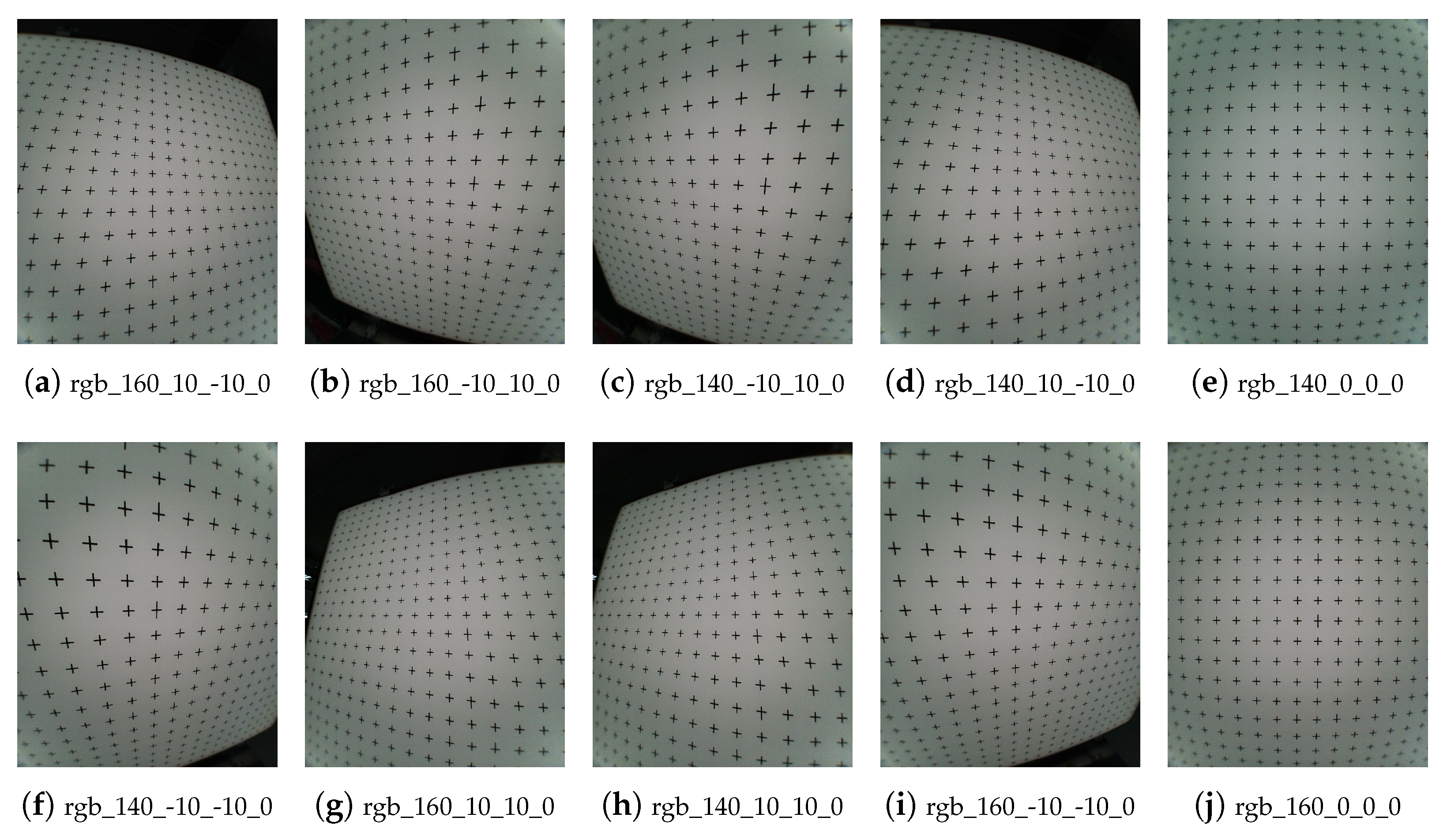
This experiment evaluates the proposed calibration framework on real-world data. Ten checkerboard images with different poses were captured using a commercial Yipin freeform lens (Yipin Optical, Shangrao, China). The checkerboard was placed at different positions and orientations to provide sufficient coverage of the field of view, particularly near the image boundaries. Figure 5 shows the acquired calibration images.

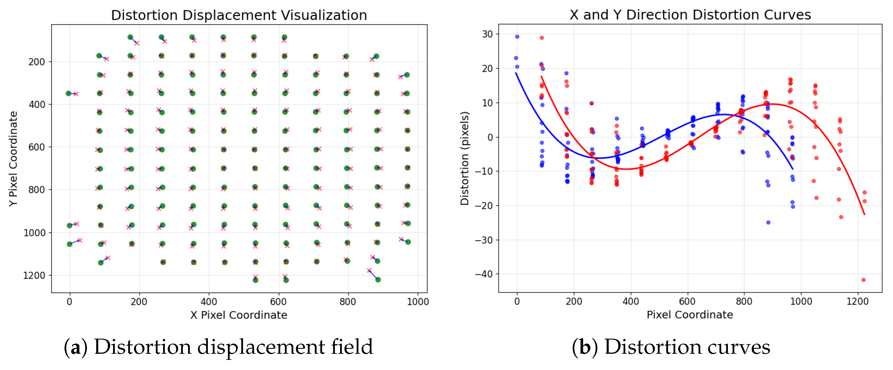
The tested lens adopts a 1G4P optical structure (one glass element and four plastic elements), with an effective focal length of 0.77 mm and a wide asymmetric field of view (120° horizontally and 130° vertically). Zemax OpticStudio 19.4 simulations indicate pronounced nonlinear distortion across the image plane, reaching approximately 14.99% near the image boundary, as shown in Figure 6.

To investigate how these distortion characteristics appear in real observations, the initial distortion field was estimated from the detected checkerboard corners before calibration.

Figure 7 presents the initial distortion field estimated from the captured calibration images. The distortion exhibits clear spatial non-uniformity and directional asymmetry. The distortion ranges from $-25.01$ to $29.33$ pixels in the X direction and from $-41.75$ to $28.88$ pixels in the Y direction. These observations are consistent with the trends predicted by the optical simulation and further demonstrate the limitations of conventional symmetric distortion models when applied to freeform lenses.

3.3.2. Quantitative Analysis of Reprojection Error

Table 6. Reprojection errors across 10 views on the YP dataset (pixels).

View ID	Zhang	BabelCalib	McCalib	MLS	TPS	Ours
V0	1.95	1.912	1.68	0.43	0.58	0.26
V1	2.07	1.852	1.68	0.69	0.62	0.27
V2	2.15	1.907	1.68	0.65	0.65	0.26
V3	2.03	1.839	1.72	0.72	0.60	0.27
V4	1.79	1.553	1.75	0.73	0.56	0.29
V5	1.77	1.700	1.83	0.39	0.52	0.25
V6	2.20	1.972	1.82	0.53	0.64	0.27
V7	2.14	1.882	1.80	0.60	0.70	0.27
V8	2.03	1.704	1.74	0.67	0.63	0.26
V9	1.97	1.674	1.69	0.72	0.59	0.29
Overall	2.44	1.805	1.439	0.48	0.67	0.24

Note: Per-view values are the mean reprojection errors (MSE); Overall is the global RMSE.

shows the reprojection errors and overall RMSE for each method across 10 real views. The proposed method uses a single bicubic B-spline surface with a KDE-based adaptive knot placement strategy. It achieves an overall RMSE of 0.24 pixels, outperforming all compared methods.

Zhang’s method, which uses a polynomial distortion model, has an overall RMSE of 2.444 pixels. Its per-view errors range from 1.77 to 2.20 pixels. This reflects the inherent limitation of traditional parametric models in representing complex asymmetric distortions. BabelCalib and McCalib use more advanced optimization strategies, such as hierarchical back-projection initialization and global bundle adjustment. They improve over Zhang’s method, but their errors are still much higher than those of non-parametric methods. This again shows that better optimization cannot fully compensate for limited model expressiveness.

Among non-parametric methods, MLS uses local weighted interpolation. It achieves an overall RMSE of 0.48 pixels, which is about 67% to 81% lower than parametric methods. However, its per-view errors range from 0.39 to 0.73 pixels. This large fluctuation reflects the sensitivity of local interpolation methods to data distribution and their weak global consistency. TPS fits two independent thin-plate spline surfaces to establish a smooth mapping from distorted coordinates to ideal coordinates. Its overall RMSE is 0.67 pixels.The proposed method reduces the overall RMSE by about 50% (from 0.48 to 0.24) compared to MLS and by about 64% (from 0.67 to 0.24) compared to TPS. These results demonstrate the effectiveness of the bicubic B-spline representation and the adaptive knot placement strategy on real-world complex distortion data.

3.3.3. Qualitative Evaluation of Distortion Rectification Performance

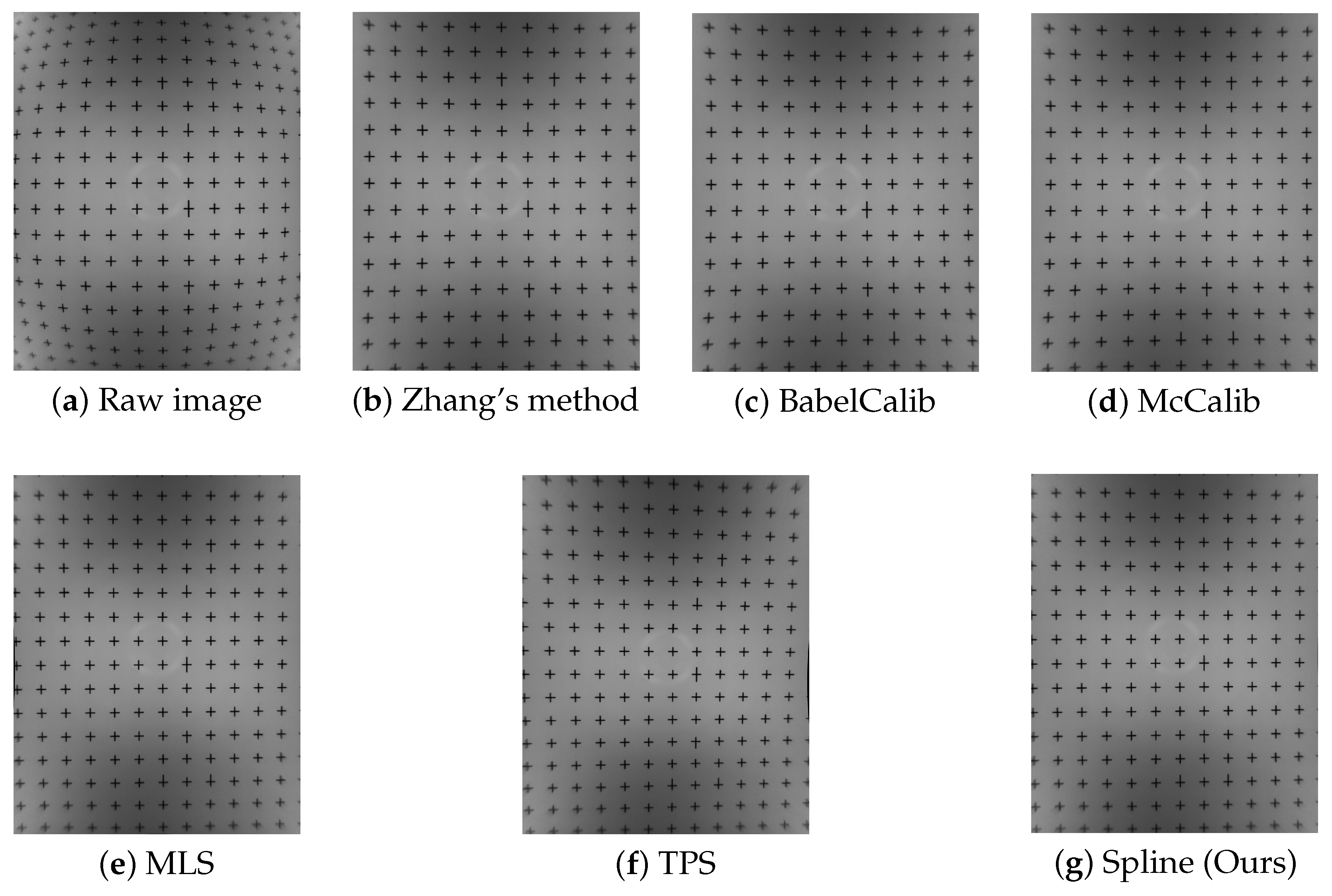
To qualitatively and quantitatively evaluate the distortion rectification performance, we present a visual comparison in Figure 8 and summarize representative geometric quality metrics in

Table 7. Comparison of geometric quality metrics for different rectification methods.

Method	Straightness RMSE	Spacing CV	Orthogonality Error	Distortion Smoothness
Raw image	11.161	0.111	5.82	0.095
Zhang’s method	3.850	0.072	2.94	0.061
BabelCalib	2.650	0.056	2.15	0.049
McCalib	2.420	0.053	1.95	0.045
MLS	1.980	0.047	1.60	0.038
TPS	1.780	0.043	1.42	0.032
Spline (Ours)	1.420	0.036	1.12	0.025

. The evaluated metrics include Straightness RMSE (lower is better), Spacing Coefficient of Variation (Spacing CV; lower indicates more uniform grid spacing), Orthogonality Error (lower indicates better preservation of right angles), and Distortion Field Smoothness (lower indicates smoother deformation).

As shown in Table 7, the raw distorted image exhibits significant geometric deviations across all evaluated metrics, confirming the presence of strong nonlinear distortion. After rectification, all methods substantially improve geometric regularity, as reflected by the reduced straightness error and improved spacing uniformity. Among the parametric calibration methods, Zhang’s method achieves limited correction due to its simplified distortion model, leading to noticeable residual curvature. BabelCalib and McCalib further improve geometric accuracy, yielding lower straightness and orthogonality errors. However, as illustrated in Figure 8, these methods still exhibit minor local inconsistencies and slight degradation near image boundaries, suggesting limited flexibility in modeling complex spatial distortions.

Non-parametric approaches, including MLS and TPS, demonstrate improved adaptability to nonlinear distortions. MLS provides enhanced local fitting capability, resulting in reduced geometric errors, although its locally weighted formulation may introduce moderate inconsistencies in global structure. TPS, benefiting from a global smoothness constraint, achieves more coherent deformation and improved distortion field smoothness compared to MLS. Nevertheless, slight boundary artifacts and sensitivity to control point distribution can still be observed.

The proposed spline-based method achieves consistently strong performance across all metrics. In particular, it reduces straightness error and spacing variation, indicating improved geometric regularity, while maintaining lower orthogonality error for better local structural preservation. Moreover, the distortion field exhibits enhanced smoothness, reflecting more stable and globally consistent deformation.

Overall, while existing parametric methods provide reliable baseline correction and non-parametric approaches improve flexibility, the proposed method offers a balanced trade-off between local adaptability and global consistency.

3.3.4. Hold-Out View Validation

We test the generalization ability of our calibration framework using hold-out view validation on the YP dataset. Unlike the previous test that uses all ten images for calibration, we split the images into a calibration set (eight images) and a validation set (two images). To reduce the effect of a particular split, we test five different splits, where each view serves as validation once.

For each split, all methods train on the same calibration views and test on the same validation views. The validation error is the reprojection RMSE on the checkerboard corners of the unseen views.

Table 8. Hold-out view validation results on the real-world YP dataset. Eight views are used for calibration and two unseen views for validation in each split.

Method	Calibration RMSE (px)	Validation RMSE (px)	Error Increase (px)
Zhang	2.48 ± 0.09	2.71 ± 0.18	0.23
BabelCalib	1.86 ± 0.08	2.04 ± 0.15	0.18
McCalib	1.50 ± 0.07	1.68 ± 0.13	0.18
MLS	0.53 ± 0.06	0.72 ± 0.11	0.19
TPS	0.70 ± 0.05	0.86 ± 0.10	0.16
Spline (Ours)	0.27 ± 0.03	0.36 ± 0.05	0.09

shows the results.

As Table 8 shows, all methods have higher errors on unseen views than on calibration views. This means that predicting new images is harder. Our method gives the lowest validation RMSE (0.36 pixels) and the smallest performance drop (only 0.09 pixels) from calibration to validation.

Parametric methods (Zhang, BabelCalib, McCalib) produce validation errors above 1.6 pixels. Their fixed distortion models cannot capture the spatially varying and asymmetric distortion of the freeform lens. Therefore, their accuracy on unseen views stays limited.

Among non-parametric methods, MLS has a validation RMSE of 0.72 pixels and TPS has 0.86 pixels. Both improve over parametric methods, but their error increase from calibration to validation is larger than ours. This shows that local interpolation is sensitive to the distribution of calibration samples. Global splines also become less flexible where distortion changes rapidly.

Our framework gives the lowest validation error and the smallest calibration-to-validation gap. This shows that our adaptive knot placement and control-point regularization improve generalization and prevent overfitting to specific views. Also, the small standard deviation across different splits indicates that our method stays stable under different calibration-view choices.

In summary, the hold-out validation confirms that our framework fits calibration data accurately and generalizes well to new checkerboard poses. This supports its use in practical freeform lens calibration.

3.4. Spatial Residual Analysis

We analyze the reprojection residuals on the real-world YP dataset to study the spatial distribution of calibration errors. Unlike the global RMSE in Table 6, this analysis checks whether errors spread evenly or concentrate in certain image regions, especially near boundaries where freeform lens distortion is usually stronger.

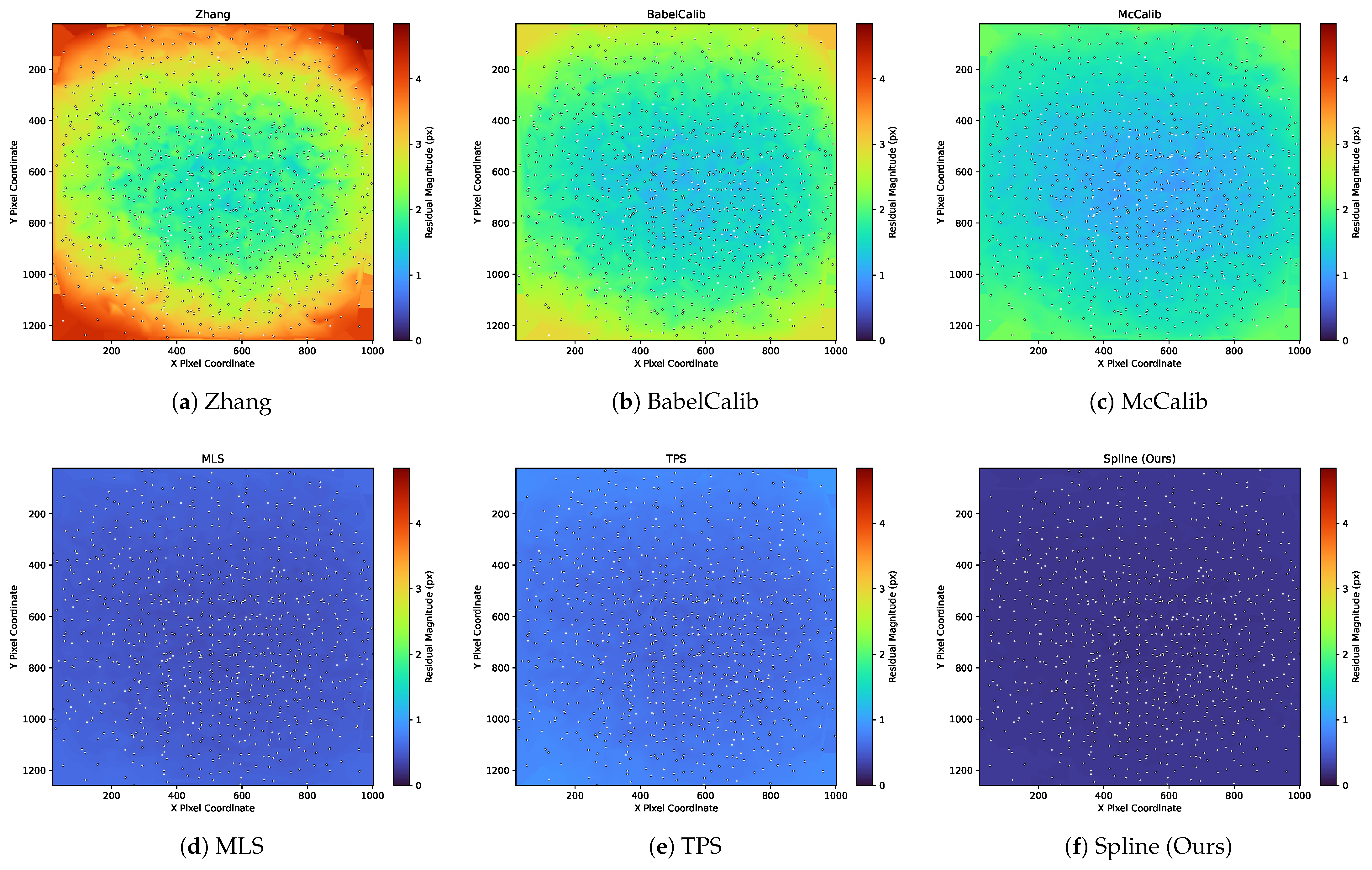
Figure 9 shows the residual heatmaps of different methods. Color intensity indicates the residual magnitude. Zhang’s method gives large residuals over a wide area, particularly near boundaries. This shows that the global polynomial model cannot fully represent the spatially varying distortion of the freeform lens. BabelCalib and McCalib reduce the overall residual level, but some high-error regions remain. Their parametric models still have limits for asymmetric distortion. MLS gives lower residuals than parametric methods, but its residual distribution is less uniform. This reflects the sensitivity of local interpolation to the layout of calibration points. TPS gives a smoother residual pattern, but noticeable residuals still appear where distortion changes rapidly. Our method gives the most uniform and lowest residual distribution across the image plane. This indicates better spatial consistency and stronger ability to model complex freeform distortion.

To compare boundary performance quantitatively, we split the image domain into a center region and an edge region. The center region is the normalized area $[0.25,0.75]\times [0.25,0.75]$, and the rest is the edge region.

Table 9. Center and edge reprojection errors on the real-world YP dataset.

Method	Center RMSE (px)	Edge RMSE (px)	Increase (px)
Zhang	2.180	3.322	1.142
BabelCalib	1.647	2.359	0.712
McCalib	1.341	1.797	0.456
MLS	0.465	0.541	0.076
TPS	0.644	0.772	0.129
Spline (Ours)	0.236	0.256	0.019

Note: Bold values indicate the best calibration performance.

lists the RMSE values in both regions. The edge-to-center increase is:

$${\mathrm{\Delta }}_{\mathrm{edge}-\mathrm{center}}={\mathrm{RMSE}}_{\mathrm{edge}}-{\mathrm{RMSE}}_{\mathrm{center}}.$$

(44)

As Table 9 shows, all methods have higher errors at the edge than at the center. This is expected because the boundary area of the freeform lens has stronger nonlinear distortion and fewer stable calibration constraints. Among parametric methods, Zhang gives the largest edge error (3.322 pixels) and the largest edge-center increase (1.142 pixels). BabelCalib and McCalib reduce the increase to 0.712 and 0.456 pixels, but their edge errors stay high. This confirms that better optimization alone cannot fix the limited expressiveness of the distortion model.

For non-parametric methods, MLS and TPS greatly reduce both center and edge errors. However, MLS still has a larger edge-center increase than our method. This suggests that local interpolation becomes less stable near boundaries where calibration points are sparse. TPS also gives a larger edge error because its global smoothness constraint may over-smooth the highly distorted boundary regions. Our method achieves the lowest center RMSE (0.236 pixels) and the lowest edge RMSE (0.256 pixels). More importantly, its edge-center increase is only 0.019 pixels, which is much smaller than that of all other methods.

These results show that our adaptive B-spline calibration framework reduces the overall reprojection error and improves spatial error uniformity. The adaptive knot placement strategy allocates modeling capacity based on how distortion changes across the image. The regularized control-point estimation suppresses unstable boundary oscillations. As a result, our method maintains robust calibration accuracy in both the center and boundary regions of the freeform lens image.

3.5. Ablation Studies

3.5.1. Ablation Study on Knot Generation

This section validates the proposed kernel density estimation (KDE)-based knot generation strategy by comparing it against conventional uniform placement and intentionally pathological configurations. The objective is to demonstrate its necessity for maintaining numerical stability (measured by design matrix condition numbers, rank, and inactive columns) and achieving high calibration accuracy.

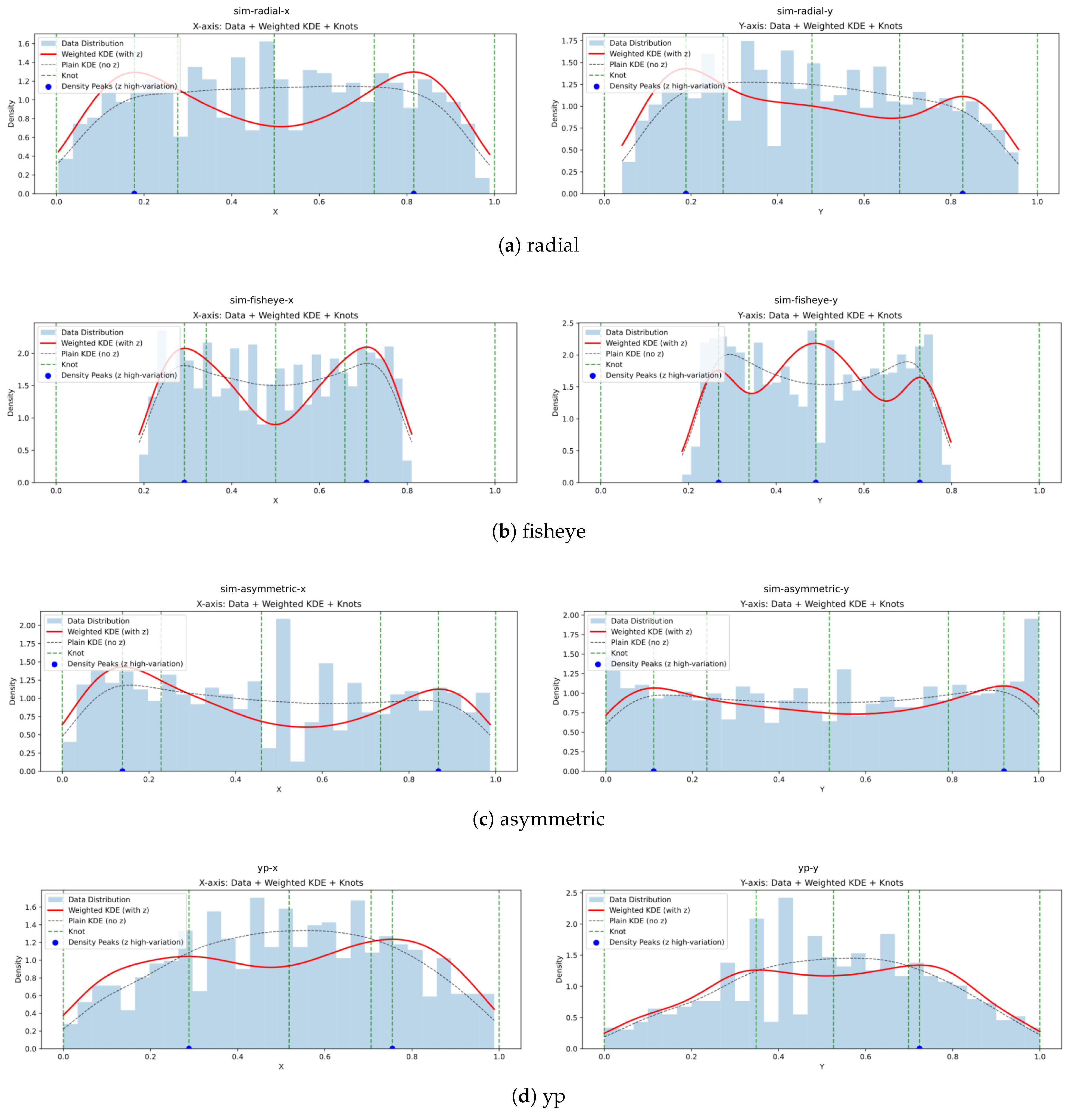
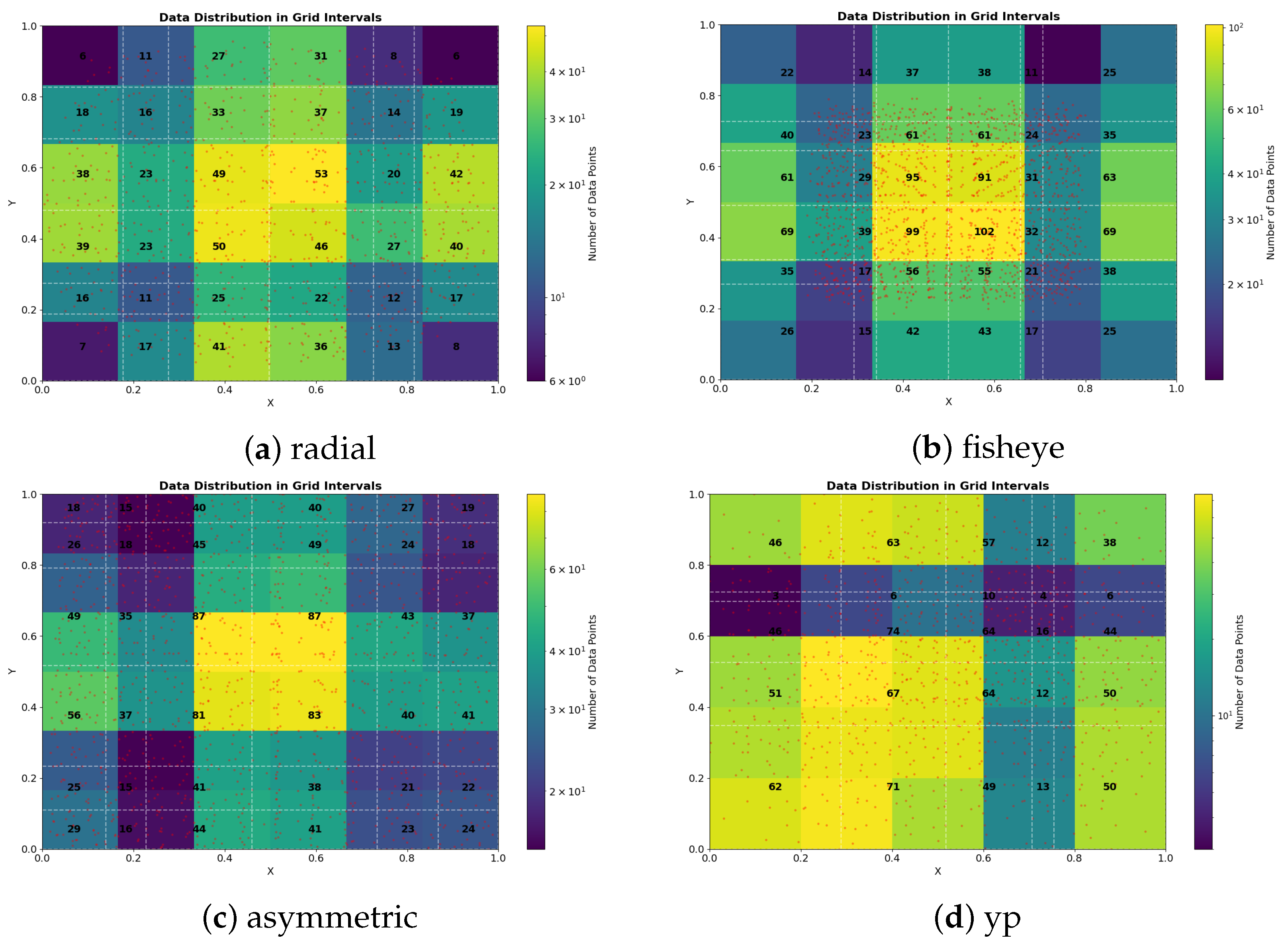
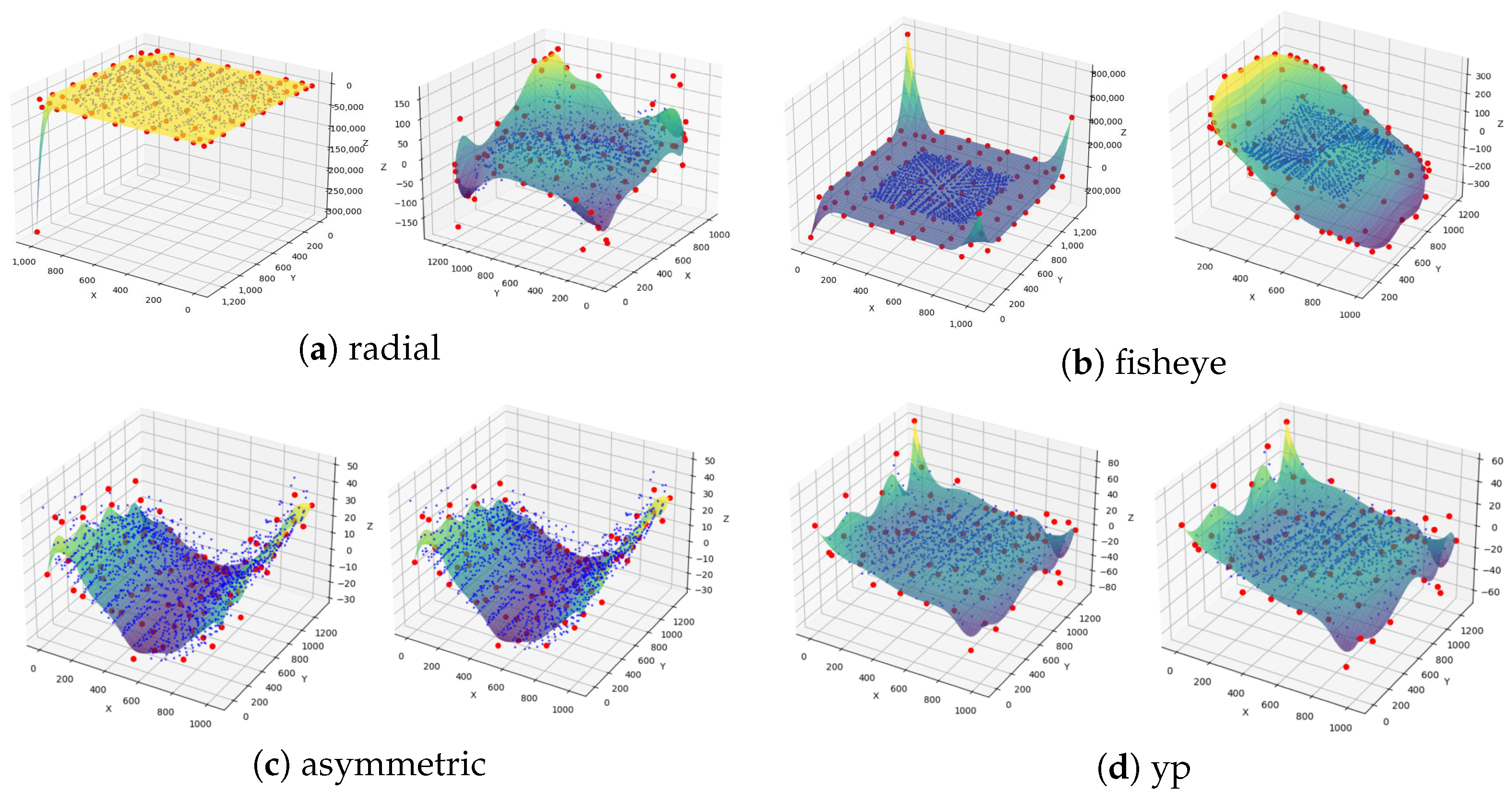
To visualize the spatial variation of distortions, Figure 10 illustrates the distortion vector distributions along the principal directions. The profiles reveal significant local complexity, particularly exhibiting stronger distortions near the periphery. As shown in Figure 11, the proposed KDE method dynamically allocates knots denser in these high-variation regions. In contrast, uniform placement ignores the underlying structural complexity, risking the creation of empty knot intervals in regions with sparse data support.

The quantitative baseline comparison (

Table 10. Condition numbers and reconstruction errors for uniform vs KDE-Based knot placement.

Dataset	KDE-Generated Knots		Uniform Knots		Reconstruction Error (px)
	X-Dir	Y-Dir	X-Dir	Y-Dir	KDE	Uniform
radial	$\mathbf{2.81}\times {\mathbf{10}}^{\mathbf{4}}$	$\mathbf{7.80}\times {\mathbf{10}}^{\mathbf{3}}$	$1.80\times {10}^5$	$7.66\times {10}^4$	$\mathbf{0.393}$	$0.673$
fisheye	$\mathbf{1.53}\times {\mathbf{10}}^{\mathbf{4}}$	$\mathbf{6.95}\times {\mathbf{10}}^{\mathbf{4}}$	∞	∞	$\mathbf{0.797}$	$1.119$
asymmetric	$\mathbf{2.03}\times {\mathbf{10}}^{\mathbf{2}}$	$\mathbf{1.94}\times {\mathbf{10}}^{\mathbf{2}}$	$5.77\times {10}^2$	$5.77\times {10}^2$	$\mathbf{0.444}$	$0.735$
yp	$\mathbf{9.69}\times {\mathbf{10}}^{\mathbf{1}}$	$\mathbf{8.67}\times {\mathbf{10}}^{\mathbf{1}}$	$3.16\times {10}^2$	$3.16\times {10}^2$	$\mathbf{0.236}$	$0.412$

Note: Bold values indicate the best calibration performance.

) confirms that KDE-generated knots yield significantly lower condition numbers and reprojection errors across all datasets.

Notably, for severe distortions like the Simulated fisheye, uniform placement results in a singular matrix (condition number ∞) due to localized data sparsity, whereas KDE maintains numerical feasibility and sub-pixel accuracy.

To explicitly test the boundaries of the stability conditions derived before, we further applied intentionally pathological knot configurations to the real YP dataset using identical optimization settings. As summarized in

Table 11. Analysis of knot placement and matrix degeneracy on the yp dataset.

Knot Configuration	Rank	Zero Cols	Cond(A) (dx/dy)	Min. Singular Val.	Empty Intervals	RMSE
Proposed KDE	64/64	0/0	84.85/70.99	0.0741/0.0857	0/0	0.236
Uniform	64/64	0/0	297.93/297.93	0.0230/0.0230	0/0	0.412
Pathological boundary	44/64	10/10	∞/∞	0/0	2/2	2.1756
Near repeat	64/64	0/0	64.01/64.01	0.0699/0.0699	3/2	0.4772
One-side right	64/64	0/0	64.00/64.00	0.0699/0.0699	3/2	0.4759
Left edge	22/64	40/40	∞/∞	0/0	4/4	1.4864
Nonuniform left	22/64	40/40	∞/∞	0/0	4/4	1.5135

Note: Bold values indicate the best calibration performance.

, while the KDE method preserves full rank (64/64) with zero inactive columns, pathological configurations clearly induce degeneracy.

Insufficient boundary coverage (pathological_boundary) reduces the design-matrix rank to $44/64$, introducing 10 zero columns. More extreme edge-concentrated cases (left_edge) further drop the rank to $22/64$ with 40 zero columns and infinite condition numbers, completely destroying the basis support. Even configurations that maintain full rank (near_repeat) exhibit empty knot intervals, leading to degraded calibration accuracy. These results empirically validate that the proposed stability-aware KDE strategy is essential not only for improving fitting accuracy but for fundamentally preserving observability and robustness in freeform lens calibration.

3.5.2. Ablation Study on KDE Bandwidth Selection

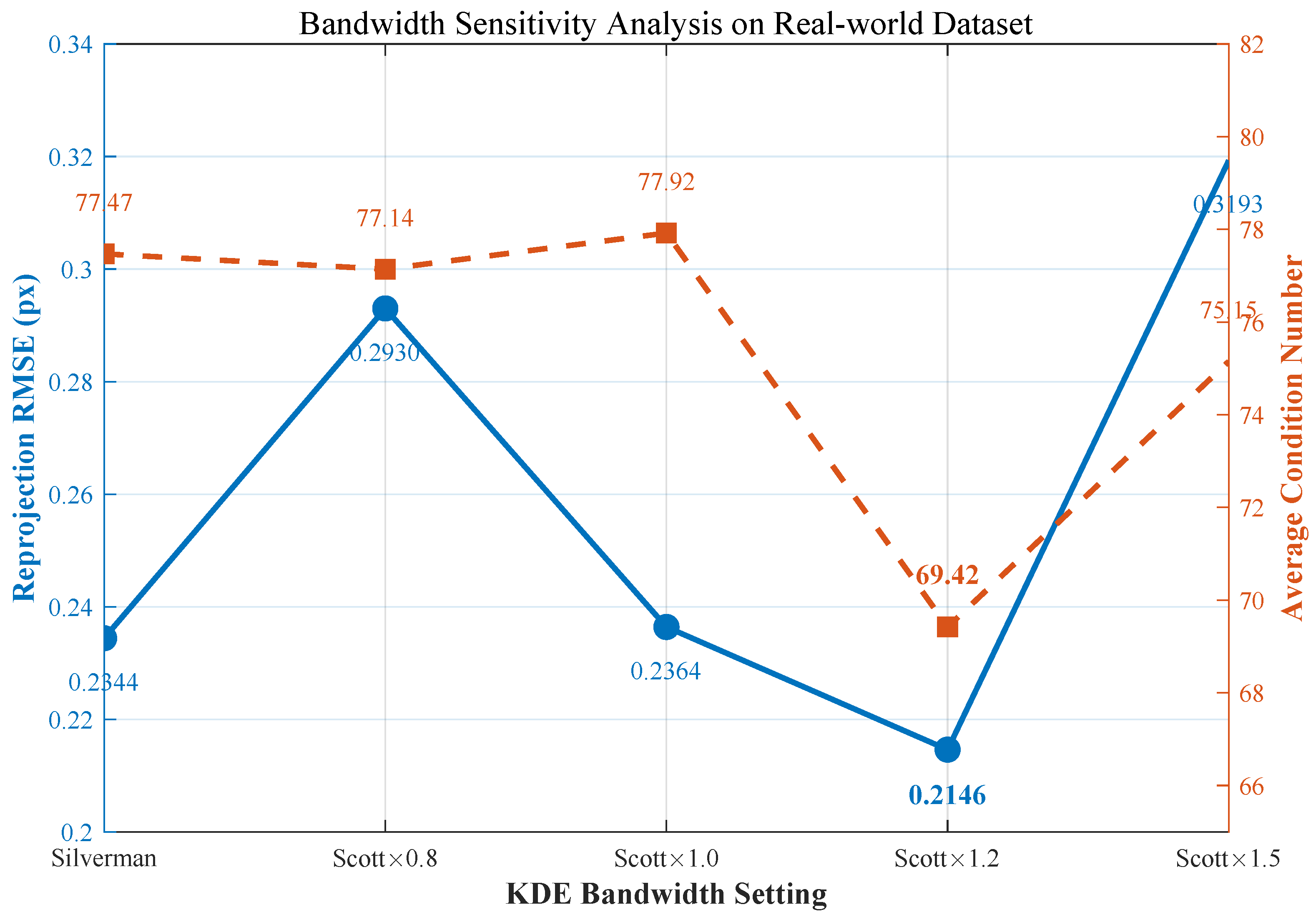
The knot generation strategy relies on a weighted one-dimensional Gaussian KDE. While Scott’s rule serves as the default bandwidth initializer, the non-uniform distribution of calibration points necessitates evaluating the method’s sensitivity to bandwidth variations. To this end, we conducted an ablation study on the yp dataset, keeping all other parameters (initial estimation, regularization, grid size, and optimization settings) constant. We compared five bandwidth settings: Silverman, Scott $\times 0.8$, Scott$\times 1.0$, Scott$\times 1.2$, and Scott$\times 1.5$.

As illustrated in Figure 12, the proposed method remains numerically stable across all tested bandwidths. Matrix-stability tracking confirmed that all settings preserved full effective rank (64/64) and produced zero inactive columns, verifying that the generated knot vectors consistently satisfy the support requirements derived above.

However, the final reprojection accuracy exhibits sensitivity to bandwidth selection. Scott $\times 1.2$ yields the lowest RMSE of 0.2146 pixels, outperforming both the default Scott setting (0.2364 pixels) and Silverman’s rule (0.2344 pixels). Conversely, under-smoothing (Scott $\times 0.8$) and over-smoothing (Scott $\times 1.5$) noticeably degrade calibration quality. These findings confirm that while Scott’s rule provides a robust baseline, a mild increase over the default bandwidth further optimizes fitting performance for real-world asymmetric distortions.

3.5.3. Ablation Study on Weighting Strategies

During B-spline control point optimization, the weight assigned to each sampled distortion vector dictates its contribution to the loss function. We evaluated four weighting strategies on the yp dataset:

• Uniform (Baseline):Assigns an equal weight ($w_i=1$) to all points, assuming uniform reliability.
• Magnitude-based: Weights are proportional to the initial residual magnitude, prioritizing regions with larger fitting errors.
• Gradient-based: Fit a local plane using k nearest neighbors to obtain the gradient magnitude $\parallel \nabla z\parallel$ as weight, focusing on regions with dramatic surface variations.
• Local Std (Proposed): Weights are derived from the local standard deviation within a sliding window, suppressing random noise while preserving structural features.

All strategies were initialized from a similar state (RMSE ≈ 5.05 pixels). As summarized in

Table 12. Calibration accuracy under different weighting strategies (yp Dataset).

Weighting Mode	Initial RMSE	Final RMSE	Improvement
Uniform	5.0582	0.4120	-
Magnitude	5.0567	0.2712	34.17%
Gradient	5.0560	0.2747	33.33%
Local Std	5.0522	0.2363	42.65%

, the proposed Local Std strategy delivers the best performance, reducing the final RMSE to 0.2363 pixels—a 42.65% improvement over the Uniform baseline. While Magnitude and Gradient strategies also achieve errors below 0.28 pixels, Local Std is superior due to its statistical ability to distinguish systematic distortion from measurement noise. By assigning higher confidence to regions with stable data distributions, this spatially-aware weighting mechanism proves essential for achieving sub-pixel accuracy in complex freeform lenses.

3.5.4. Ablation Study on Control Point Regularization

This section evaluates the contribution of the proposed regularization strategy to calibration accuracy and surface robustness. The strategy combines an $L_2$ penalty on control point weights (${\lambda }_{reg}$) with a second-order finite difference smoothness constraint (${\lambda }_{smooth}$).

To determine optimal hyperparameters, a grid-search ablation was conducted on the yp dataset (

Table 13. Reprojection RMSE for different regularization parameters.

${\mathit{\lambda }}_{\mathbf{reg}}\setminus {\mathit{\lambda }}_{\mathbf{smooth}}$	0	1 $\times {10}^{-4}$	1 $\times {10}^{-3}$	1 $\times {10}^{-2}$	1 $\times {10}^{-1}$
0	0.2298	0.2417	0.2394	0.3709	0.9884
1 $\times {10}^{-5}$	0.2412	0.2419	0.2387	0.3653	0.9888
1 $\times {10}^{-4}$	0.2425	0.2433	0.2372	0.3590	0.9849
1 $\times {10}^{-3}$	0.2401	0.2587	0.2364	0.3344	0.9823
1 $\times {10}^{-2}$	0.3029	0.3036	0.3097	0.3575	0.8222

).

The results indicate that ${\lambda }_{smooth}$ primarily balances model complexity and accuracy. While the absolute minimum RMSE (0.2298 pixels) occurs at ${\lambda }_{reg}={\lambda }_{smooth}=0$, this unconstrained state is highly susceptible to overfitting induced by corner detection noise. A moderate constraint (${\lambda }_{smooth}={10}^{-3}$) effectively suppresses local non-physical oscillations, whereas excessive constraints (${\lambda }_{smooth}\ge {10}^{-1}$) cause underfitting by over-smoothing complex distortions.The $L_2$ penalty (${\lambda }_{reg}$) ensures numerical completeness and structural robustness. Within the optimal ${\lambda }_{smooth}={10}^{-3}$ column, increasing ${\lambda }_{reg}$ from 0 to ${10}^{-3}$ causes only a 1.2% RMSE fluctuation, achieving a robust global optimum of 0.2364 pixels. Consequently, $({\lambda }_{reg},{\lambda }_{smooth})=({10}^{-3},{10}^{-3})$ is selected as the optimal configuration.

Using these optimal parameters, we compared the proposed method against a baseline with No Regularization (NR) across multiple datasets (

Table 14. RMS reprojection errors for different regularization strategies.

Dataset	No Regularization (NR)	Proposed
radial	0.3846	0.3927
fisheye	0.4636	0.4442
asymmetric	0.7906	0.7970
yp	0.2298	0.2364

).

Quantitatively, the RMS reprojection errors remain remarkably close across all datasets, with differences strictly within 0.01 pixels. This confirms the regularization strategy maintains baseline accuracy. Qualitatively, as shown in Figure 13, the unregularized method exhibits significant non-physical oscillations in regions with sparse calibration points or complex asymmetric components. In contrast, the proposed method effectively suppresses overfitting, consistently generating smoother and physically plausible distortion surfaces without compromising numerical precision.

4. Discussion

Our performance gains come not only from using B-spline representation. Existing B-spline methods only use spline functions for distortion interpolation after calibration. Our framework directly integrates a continuous 2D B-spline distortion field into the calibration model and jointly optimizes it with camera parameters. Jacobian-based analysis shows that stability depends on basis-function activation and parameter observability. So we introduce an adaptive knot generation strategy. This strategy does more than improve fitting accuracy. It also preserves matrix rank, maintains numerical conditioning, and enables stable optimization under non-uniform calibration point distributions. Specifically, it adjusts knot density based on local distortion changes and enforces a minimum support constraint. This reduces instability from uneven data sampling.

Unlike TPS and MLS (often used as post-processing tools), our joint optimization gives the B-spline model a more stable trade-off between local control and global consistency. TPS tends to over-smooth high-distortion regions. MLS may cause regional inconsistencies. By solving distortion modeling and camera parameter estimation together in one unified optimization, our method better balances local fitting with global geometry. Under our settings, the method shows good numerical stability.

Despite these advantages, the proposed method has several limitations that warrant further investigation.

• First, the current validation does not cover a wide range of lens types, imaging conditions, or different camera platforms. More extensive experiments are therefore needed to confirm the generalizability of our conclusions.
• Second, the performance of the method is contingent upon the quantity and distribution of the calibration data. In cases where the data are extremely sparse or highly clustered, the stability of the estimation may be compromised.
• Third, the current framework does not explicitly account for temporal variations or environmental factors, such as temperature-induced drift or mechanical vibration. Consequently, its applicability to dynamic or complex scenarios remains limited, and further extensions are required to handle such conditions.
• Fourth, the joint optimization of camera parameters and control points incurs higher computational overhead compared to traditional parametric methods. This increased computational complexity may limit the operational efficiency of the proposed method in large-scale tasks and real-time applications that demand stringent low-latency performance.

Future work will explore multi-resolution adaptive spline representations, integrate learning-based priors to improve data efficiency, and extend to dynamic calibration scenarios, aiming to further enhance robustness while reducing computational and data dependencies.In addition, validation on multiple freeform lens systems and dynamic calibration scenarios will be conducted to better assess the general applicability of the proposed framework.

5. Conclusions

This paper proposed a calibration framework for freeform lenses using bicubic B-spline surfaces. The method combines Zhang’s initialization with an adaptive knot generation strategy based on kernel density estimation and dynamic grid adjustment. Regularization with $L_2$ and smoothness constraints is introduced to improve numerical stability.

Experiments on synthetic data show that the proposed method achieves mean reprojection errors of 0.45 pixels for symmetric distortion and 0.80 pixels for asymmetric distortion. On real-world freeform lens data, the method achieves a reprojection error of 0.24 pixels. Compared with traditional polynomial models, the B-spline representation offers greater flexibility in handling complex and asymmetric distortions. The adaptive knot placement ensures numerical stability even when calibration data are unevenly distributed. The regularization strategy prevents overfitting and produces physically plausible distortion surfaces. These results validate that combining B-spline surface modeling with adaptive optimization provides a practical and effective solution for freeform lens calibration.

References

1. Afanaseva, O.; Solomashenko, A.; Shishova, M.; Timashova, L.; Sagatelyan, G.; Tsyganov, I. Design of freeform elements with a large exit pupil for AR display. Optik 2024, 319, 172101. [Google Scholar] [CrossRef]
2. Kumar, S.; Zhong, W.; Williamson, J.; Kumar, P.; Furness, T.; Lou, S.; Zeng, W.; Jiang, X. Design, fabrication, and testing of freeform mirror-based head-up display system. Opt. Laser Technol. 2025, 186, 112653. [Google Scholar] [CrossRef]
3. Yu, J.; Mao, X. Design of off-axis four-mirror optical systems enabled by freeform optics. Photonics 2025, 12, 107. [Google Scholar] [CrossRef]
4. Ding, Y.; Zhang, N.; Yang, C. Design of freeform surface low-distortion automotive lens based on point-by-point construction. Acta Opt. Sin. 2024, 44, 223–233. [Google Scholar]
5. Wang, S.; Kong, L.; Lv, H. Advances in Measurement and Error Evaluation Technique of Optical Freeform Surfaces. Acta Opt. Sin. 2023, 43, 0822013. [Google Scholar]
6. Zhang, X.; Qiu, L.; Zhao, W.; Fu, Y.; Wang, Y.; Liu, Y. Free-form surface measurement with laser differential confocal precise positioning. Opt. Laser Technol. 2025, 183, 112325. [Google Scholar] [CrossRef]
7. Zhang, Z. A flexible new technique for camera calibration. IEEE Trans. Pattern Anal. Mach. Intell. 2000, 22, 1330–1334. [Google Scholar] [CrossRef]
8. Kannala, J.; Brandt, S. A generic camera model and calibration method for conventional, wide-angle, and fish-eye lenses. IEEE Trans. Pattern Anal. Mach. Intell. 2006, 28, 1335–1340. [Google Scholar] [CrossRef]
9. Real-Moreno, O.; Rodríguez-Quiñonez, J.C.; Sergiyenko, O.; Flores-Fuentes, W.; Castro-Toscano, M.J.; Miranda-Vega, J.E.; Mercorelli, P.; Valdez-Rodríguez, J.A.; Trujillo-Hernández, G.; Sanchez-Castro, J.J. A Quadrant Approach of Camera Calibration Method for Depth Estimation Using a Stereo Vision System. In Proceedings of the IECON 2022—48th Annual Conference of the IEEE Industrial Electronics Society; IEEE: Piscataway, NJ, USA, 2022; pp. 1–6. [Google Scholar] [CrossRef]
10. Real-Moreno, O.; Rodríguez-Quiñonez, J.C.; Flores-Fuentes, W.; Sergiyenko, O.; Miranda-Vega, J.E.; Trujillo-Hernández, G.; Hernández-Balbuena, D. Camera calibration method through multivariate quadratic regression for depth estimation on a stereo vision system. Opt. Lasers Eng. 2024, 174, 107932. [Google Scholar] [CrossRef]
11. Ma, X.; Zhu, P.; Li, X.; Zheng, X.; Zhou, J.; Wang, X.; Wai Samuel Au, K. A Minimal Set of Parameters-Based Depth-Dependent Distortion Model and Its Calibration Method for Stereo Vision Systems. IEEE Trans. Instrum. Meas. 2024, 73, 1–11. [Google Scholar] [CrossRef]
12. Rameau, F.; Park, J.; Bailo, O.; Kweon, I.S. MC-Calib: A generic and robust calibration toolbox for multi-camera systems. Comput. Vis. Image Underst. 2022, 217, 103353. [Google Scholar] [CrossRef]
13. Lochman, Y.; Liepieshov, K.; Chen, J.; Perdoch, M.; Zach, C.; Pritts, J. Babelcalib: A universal approach to calibrating central cameras. In Proceedings of the IEEE/CVF International Conference on Computer Vision, Montreal, QC, Canada, 10–17 October 2021; pp. 15253–15262. [Google Scholar]
14. Jin, Z.; Li, Z.; Gan, T.; Fu, Z.; Zhang, C.; He, Z.; Zhang, H.; Wang, P.; Liu, J.; Ye, X. A novel central camera calibration method recording point-to-point distortion for vision-based human activity recognition. Sensors 2022, 22, 3524. [Google Scholar] [CrossRef] [PubMed]
15. Zhan, N.; Zhang, X.; Ye, J.; Wang, T.; Dong, Z.; Song, Z. High-precision parameter-free optical distortion measurement and correction via digital image correlation. Opt. Laser Technol. 2024, 177, 111129. [Google Scholar] [CrossRef]
16. Yinguo, L.; Cheng, C. Distortion correction method for cameras with wide-angle lens based on nonlinear spline interpolation. CAAI Trans. Intell. Syst. 2020, 15, 1033–1039. [Google Scholar] [CrossRef]
17. Huang, L.; Wang, X.; Hou, J.; Zhou, X.; Wang, B.; Zhu, L.; Lyu, F. A Free-form Surface Distortion Correction Method and Process Based on Moving Least Squares Surface Fitting. Chinese Patent 202411229789.X, 24 November 2024. Available online: https://www.xjishu.com/zhuanli/55/202411229789.html (accessed on 10 November 2024).
18. Yu, J.; Sun, H.; Xia, Z.; Zhu, J.; Zhang, Z. Sample balancing of curves for lens distortion modeling and decoupled camera calibration. Opt. Commun. 2023, 537, 129221. [Google Scholar] [CrossRef]
19. Wang, K.; Liu, C.; Shen, S. Geometric calibration for cameras with inconsistent imaging capabilities. Sensors 2022, 22, 2739. [Google Scholar] [CrossRef]
20. Zhao, Y.; Huang, X.; Zhang, Z. Deep Lucas-Kanade Homography for Multimodal Image Alignment. In Proceedings of the 2021 IEEE/CVF Conference on Computer Vision and Pattern Recognition (CVPR), Nashville, TN, USA, 20–25 June 2021; pp. 15945–15954. [Google Scholar] [CrossRef]
21. Cao, S.Y.; Hu, J.; Sheng, Z.; Shen, H.L. Iterative Deep Homography Estimation. In Proceedings of the 2022 IEEE/CVF Conference on Computer Vision and Pattern Recognition (CVPR), New Orleans, LA, USA, 19–24 June 2022; pp. 1869–1878. [Google Scholar] [CrossRef]
22. Ye, N.; Wang, C.; Fan, H.; Liu, S. Motion Basis Learning for Unsupervised Deep Homography Estimation with Subspace Projection. In Proceedings of the 2021 IEEE/CVF International Conference on Computer Vision (ICCV), Montreal, QC, Canada, 11–17 October 2021; pp. 13097–13105. [Google Scholar] [CrossRef]
23. Shao, R.; Wu, G.; Zhou, Y.; Fu, Y.; Fang, L.; Liu, Y. LocalTrans: A Multiscale Local Transformer Network for Cross-Resolution Homography Estimation. In Proceedings of the 2021 IEEE/CVF International Conference on Computer Vision (ICCV), Montreal, QC, Canada, 11–17 October 2021; pp. 14870–14879. [Google Scholar] [CrossRef]
24. Jiang, H.; Li, H.; Han, S.; Fan, H.; Zeng, B.; Liu, S. Supervised Homography Learning with Realistic Dataset Generation. arXiv 2023, arXiv:2307.15353. [Google Scholar] [CrossRef]
25. Cattaneo, D.; Vaghi, M.; Ballardini, A.L.; Fontana, S.; Sorrenti, D.G.; Burgard, W. CMRNet: Camera to LiDAR-Map Registration. In Proceedings of the 2019 IEEE Intelligent Transportation Systems Conference (ITSC), Auckland, New Zealand, 27–30 October 2019; pp. 1283–1289. [Google Scholar] [CrossRef]
26. Yao, L.; Chen, C.; Li, X.; Yan, Z.; Zuo, W. Combining Generative and Geometry Priors for Wide-Angle Portrait Correction. arXiv 2024, arXiv:2410.09911. [Google Scholar] [CrossRef]
27. Dal Cin, A.P.; Azzoni, F.; Boracchi, G.; Magri, L. Revisiting Calibration of Wide-Angle Radially Symmetric Cameras. In Proceedings of the Computer Vision–ECCV 2024; Leonardis, A., Ricci, E., Roth, S., Russakovsky, O., Sattler, T., Varol, G., Eds.; Springer: Cham, Switzerland, 2025; pp. 214–230. [Google Scholar]
28. Zhao, K.; Lin, C.; Liao, K.; Yang, S.; Zhao, Y. Revisiting Radial Distortion Rectification in Polar-Coordinates: A New and Efficient Learning Perspective. IEEE Trans. Circuits Syst. Video Technol. 2022, 32, 3552–3560. [Google Scholar] [CrossRef]
29. Athwale, A.; Shili, I.; Bergeron, É.; Ahmad, O.; Lalonde, J.F. DarSwin-Unet: Distortion Aware Encoder-Decoder Architecture. arXiv 2025, arXiv:2407.17328. [Google Scholar]
30. Cao, M.; Yang, S.; Yang, Y.; Zheng, Y. Rolling Shutter Correction with Intermediate Distortion Flow Estimation. arXiv 2024, arXiv:2404.06350. [Google Scholar] [CrossRef]
31. Nguyen, H.; Jang, Y.M. Design and Implementation of Rolling Shutter MIMO-OFDM scheme for Optical Camera Communication System. In Proceedings of the 2021 International Conference on Information and Communication Technology Convergence (ICTC), Jeju Island, Republic of Korea, 20–22 October 2021; pp. 798–800. [Google Scholar] [CrossRef]
32. Fan, B.; Wan, Z.; Shi, B.; Xu, C.; Dai, Y. Unified Video Reconstruction for Rolling Shutter and Global Shutter Cameras. IEEE Trans. Image Process. 2024, 33, 6821–6835. [Google Scholar] [CrossRef] [PubMed]
33. Kawanishi, H.; Hara, Y.; Tsubouchi, T.; Ohya, A. Calibration of lens distortion for super-wide-angle stereo vision. In Proceedings of the 2015 IEEE International Conference on Automation Science and Engineering (CASE); IEEE: Piscataway, NJ, USA, 2015; pp. 843–848. [Google Scholar]
34. Hu, H.; Qian, B.; Fan, L. An accurate underwater camera calibration method based on a nonparametric distortion model. Measurement 2025, 258, 119024. [Google Scholar] [CrossRef]
Figure 1. Schematic diagram of the overall calibration pipeline. The process begins with initial parameter estimation using Zhang’s method, followed by B-spline surface modeling with stability-aware knot vector generation, and concludes with joint optimization of all parameters to achieve accurate distortion calibration and correction.
Applsci 16 05775 g001
Figure 2. Simulated undistorted corner point data across four different viewpoints: (a) Viewpoint 1; (b) Viewpoint 2; (c) Viewpoint 3; (d) Viewpoint 4. Red dashed lines indicate image boundaries, blue lines represent the horizontal grid lines of the original chessboard, red dots represent corner points within the field of view (FOV), and gray dots denote the original chessboard corners located outside the FOV.
Applsci 16 05775 g002
Figure 3. Distortion patterns at Viewpoint 0 for three models. Each subfigure consists of two parts: the left shows distortion displacement, where green dots indicate ideal points, red crosses indicate distorted points, and blue vectors represent displacement in pixel coordinates; the right shows distortion curves, where blue and red curves correspond to poly3 fits for x and y directions, and scattered points represent actual Δ x and Δ y .
Applsci 16 05775 g003
Figure 4. Performance degradation curves showing the relationship between noise level σ and calibration RMSE.
Applsci 16 05775 g004
Figure 5. Checkerboard images used for calibration. Subplot labels indicate the shooting distance [mm], pitch angle, and yaw angle, respectively.
Applsci 16 05775 g005
Figure 6. Optical distortion profiles of the commercial Yipin freeform lens obtained from Zemax simulations: (a) horizontal distortion profile; (b) vertical distortion profile.
Applsci 16 05775 g006
Figure 7. Initial distortion field of the YP dataset for view 0, presented in the same format as Figure 3.
Applsci 16 05775 g007
Figure 8. Visual comparison of distortion rectification results.
Applsci 16 05775 g008
Figure 9. Spatial residual heatmaps on the real-world YP dataset. Warmer colors mean larger reprojection residuals. Our method gives the lowest and most uniform residual distribution.
Applsci 16 05775 g009
Figure 10. Distribution of distortion vectors along the x / y directions. Peaks indicate high distortion variation requiring denser knot placement.
Applsci 16 05775 g010
Figure 11. Knot vector distributions generated by the proposed KDE method across the four datasets. Numbers indicate the count of corner points within each knot interval.
Applsci 16 05775 g011
Figure 12. Bandwidth sensitivity analysis for KDE-based knot generation on the yp dataset. The dual Y-axis plot illustrates the variation of reprojection RMSE and average condition number across different bandwidth settings.
Applsci 16 05775 g012
Figure 13. Comparison of reconstructed distortion surfaces across four datasets. In each subplot, the left portion represents the raw surface without regularization, while the right portion displays the smoothed surface constrained by regularization.
Applsci 16 05775 g013