Physics-Informed Machine Learning Model (NitroPINN) for Nitrogen Content Prediction in Crude Steel Produced in BOF

Abstract

Nitrogen control in basic oxygen furnace (BOF) steelmaking is critical, as dissolved nitrogen concentrations exceeding 30–40 ppm detrimentally affect the mechanical properties and formability of low-carbon steel products; however, no prior study has applied a physics-informed machine learning model to nitrogen prediction at this process stage. A NitroPINN model was developed incorporating a multiplicative prediction structure that embeds Sievert’s law equilibrium, Wagner interaction coefficients, and Byrne–Belton surface blockage theory directly into the model. The model was trained and evaluated on 66 matched industrial heats from a top-blown 170-ton BOF converter, characterized by 16 physics-informed features, and benchmarked against ridge regression and a pure multilayer perceptron (MLP) under five-fold cross-validation. The NitroPINN achieved the lowest mean absolute error (MAE = 5.60 ppm) and mean absolute percentage error (MAPE = 27.2%) among the three models, whilst the learned equilibrium attainment factor η averaged 0.456 ± 0.028, consistent with sub-equilibrium nitrogen conditions imposed by intense CO flushing during oxygen blowing. All three models exhibited comparable overall accuracy, confirming that dataset size constitutes the principal performance bottleneck. The primary advantage of the NitroPINN lies in its physical interpretability, constraining predictions to metallurgically plausible ranges and providing a transparent decomposition into thermodynamic and kinetic contributions.

1. Introduction

Nitrogen control in steel production represents one of the most critical metallurgical challenges, as even trace quantities of dissolved nitrogen profoundly influence the mechanical properties, formability, and service performance of finished steel products [1]. In low-carbon steels destined for automotive deep-drawing applications, nitrogen contents exceeding 30–40 ppm are known to impair deep drawability by promoting strain aging, whereby interstitial nitrogen atoms pin mobile dislocations and thereby increase the yield strength whilst reducing ductility [2]. The precipitation of aluminum nitride (AlN) particles during recrystallization annealing governs the crystallographic texture development that determines the Lankford r-value, and excessive nitrogen levels shift the texture from the desirable {111} grain towards less favorable orientations [3]. In structural steels, nitrogen-induced age hardening compromises impact toughness, particularly at sub-ambient temperatures, and promotes brittle fracture through the formation of iron nitride (Fe₄N) precipitates along grain boundaries. Bazaleeva [4] comprehensively reviewed the mechanisms through which nitrogen influences both austenitic and ferritic steel grades, demonstrating that the dual role of nitrogen—beneficial at controlled levels in high-nitrogen austenitic steels yet deleterious in conventional low-alloy grades—necessitates precise prediction and control throughout the steelmaking process chain. In typical BOF steelmaking operations, the nitrogen content of crude steel before tapping ranges between 20 and 60 ppm, depending on the raw material composition, blowing practice, and tapping conditions [5]. The imperative to predict and control this narrow concentration range with high accuracy has driven substantial research interest in both mechanistic and data-driven modeling approaches.

The thermodynamics of nitrogen dissolution in liquid iron and steel are described by Sievert’s law, which relates the equilibrium nitrogen solubility to the partial pressure of molecular nitrogen above the melt [6]. The dissolution reaction, (1), is characterized by a standard Gibbs energy change (2) where T is the absolute temperature in Kelvin [7]. The equilibrium constant for the reaction (1) is expressed in the form given by Equation (3) [8]. The equilibrium constant is conventionally expressed in logarithmic form as Equation (4), derived by Shamsuddin [7] for steelmaking temperatures in the range of 1823–1973 K.

¹/₂ N_2(g) = [N]

(1)

ΔG° = −3590 − 23.89 T [J·mol⁻¹]

(2)

$$K_N={\displaystyle \frac{a_N}{{\left(p_{N_2}\right)}^{\frac{1}{2}}}}={\displaystyle \frac{f_N\left[\%N\right]}{\sqrt{p_{N_2}}}}$$

(3)

$$\log K_N=-{\displaystyle \frac{375}{\mathrm{T}}}-1.154$$

(4)

The activity coefficient of nitrogen f_N accounts for the non-ideal interactions between dissolved nitrogen and other solute elements in the steel bath and is calculated using the Wagner interaction parameter formalism (5) [9,10].

$$\log f_N=e_N^C·\left[C\right]+e_N^{Mn}·\left[Mn\right]+e_N^{Si}·\left[Si\right]+e_N^P·\left[P\right]+e_N^S·\left[S\right]+e_N^O·\left[O\right]$$

(5)

The interaction coefficients, determined experimentally by [10] and confirmed by [11,12], indicate that carbon ($e_N^C$ = 0.13), silicon ($e_N^{Si}$ = 0.047), phosphorus ($e_N^P$ = 0.045) and sulfur ($e_N^S$ = 0.007) increase the nitrogen activity coefficient and thereby decrease the equilibrium solubility, whereas manganese ($e_N^{Mn}$ = −0.02) and oxygen ($e_N^O$ = −0.12) decrease f_N and promote nitrogen absorption [9]. These thermodynamic relationships provide the fundamental framework upon which the physics-informed model developed in the present study is constructed.

Whilst thermodynamic equilibrium defines the theoretical upper bound for nitrogen solubility, the actual nitrogen content in BOF crude steel is governed primarily by kinetic factors that prevent the system from reaching equilibrium [13]. The rate of nitrogen transfer across the gas–metal interface is strongly influenced by the presence of surface-active elements, principally dissolved oxygen and sulfur, which adsorb onto the liquid iron surface and block potential reaction sites for nitrogen dissociation [14]. This surface blockage effect is quantified through the relationship (6) [15].

$$\left(1-\theta \right)={\displaystyle \frac{1}{1+260·\left(\%O+\frac{\%S}{2}\right)}}$$

(6)

In a top-blown BOF operating with min. 99.5% purity oxygen, the effective partial pressure of nitrogen above the bath is exceedingly low (1.0–5.1 kPa), being limited to trace nitrogen impurities in the pure oxygen supply and atmospheric entrainment through the BOF vessel mouth [16,17]. The dominant mechanism for nitrogen removal during the oxygen blow is the physical entrainment and stripping of dissolved nitrogen by CO gas bubbles generated during vigorous decarburization. The reaction kinetics in steel production were investigated, and it was demonstrated that the rate of denitrification is proportional to the volumetric rate of CO production, which in turn depends on the carbon content of the bath and the rate of oxygen injection [13]. During a typical 17 min oxygen blow in which the carbon content decreases from approximately 4.4% in pig iron to 0.03–0.07% in crude steel, the intense CO boiling creates a large gas–metal interfacial area that facilitates nitrogen desorption and transport to the gas phase [17,18].

This kinetic framework underpins the physical motivation for several features employed in the present NitroPINN model, including the decarburization rate and the Byrne–Belton [15] surface blockage parameter.

Despite the well-established thermodynamic and kinetic foundations described above, purely mechanistic models for nitrogen prediction in BOF steelmaking encounter significant practical limitations [19,20,21,22]. The simultaneous dependence of the final nitrogen content on raw material variability (pig iron composition, scrap quality, and nitrogen introduced during desulfurization), operational parameters (blowing time, oxygen flow rate, lance height), slag composition and its physico-chemical properties, and the complex multiphase fluid dynamics within the converter renders first-principles modeling exceedingly difficult to calibrate and validate under industrial conditions [21]. Nam et al. [22] developed an integrated mathematical model for nitrogen control in oxygen steelmaking that coupled thermodynamic equilibrium with mass transfer kinetics, yet acknowledged that the model required continuous recalibration to accommodate plant-specific variations. Yoon et al. [23] presented a nitrogen prediction model for a 320-ton converter combining thermodynamic and kinetic sub-models, but reported prediction errors exceeding 15 ppm for certain heat categories. These limitations have driven growing interest in mechanism–data hybrid approaches, in which physical sub-models are coupled with data-driven components to balance mechanistic rigor with practical adaptability; for example, Li et al. [24] demonstrated that such a hybrid architecture substantially reduced both the energy consumption prediction error and carbon emission estimation uncertainty in converter steelmaking relative to purely empirical models. These limitations have motivated the application of data-driven machine learning (ML) approaches to nitrogen prediction. Patra et al. [19] employed artificial neural networks for nitrogen prediction during argon oxygen decarburization (AOD) of stainless steel, achieving improved accuracy over empirical correlations. Liu et al. [20] developed a stacked autoencoder with sparse Bayesian regression for end-point prediction in steelmaking, demonstrating that deep learning architectures can capture non-linear relationships inaccessible to linear models. More recently, Liu et al. [25] developed a dynamic flame feature-driven deep learning model for real-time end-point prediction in BOF steelmaking, achieving improved accuracy through the extraction of temporal process signatures—an approach that further underscores the growing application of advanced neural architectures to converter process control. Similarly, Niu et al. [26] applied a multi-target adversarial transfer learning framework based on the TabTransformer architecture to BOF end-point composition prediction, demonstrating that transfer learning can effectively compensate for the limited labeled data characteristic of industrial steelmaking datasets. Zhang and Yang [21] conducted a comprehensive review of ML applications in steelmaking process modeling, identifying neural networks, support vector machines, and ensemble methods as the most effective algorithms, whilst noting that data quality and feature engineering remain critical bottlenecks. A recent review by Pawlik et al. [27] further surveyed the progress, challenges, and emerging opportunities of artificial intelligence in steelmaking, identifying physics-informed and hybrid modeling strategies as the most promising directions for overcoming the persistent limitations of purely data-driven approaches in industrial deployment.

Physics-informed neural networks (PINNs), formalized by Raissi et al. [28], represent a paradigm shift in scientific machine learning by embedding known physical laws directly into the neural network training process. Rather than relying solely on data-driven loss minimization, PINNs augment the standard data-fitting objective with additional loss terms that penalize violations of governing differential equations, conservation laws, or constitutive relationships. Karniadakis et al. [29] provided a comprehensive review of physics-informed machine learning in Nature Reviews Physics, demonstrating that PINNs achieve superior generalization performance in data-scarce regimes precisely because the embedded physics constrains the solution space to physically plausible regions. This characteristic is particularly advantageous in metallurgical applications, where the collection of large, high-quality datasets is constrained by the cost of industrial sampling campaigns and the inherent variability in production conditions [30,31,32,33]. Cuomo et al. [31] further reviewed the state of scientific machine learning through PINNs, emphasizing their effectiveness in inverse problems and parameter identification tasks where traditional data-driven models are prone to overfitting. Recent application-oriented studies have further extended the PINN framework to address long-time-scale behavior through sequential training strategies [34,35], as well as to inverse parameter identification in geotechnical engineering under noisy and limited observational data [36]—contexts that share the methodological challenge of constraining a neural network to physically plausible solutions when the available data are insufficient to fully determine the model parameters from data alone. Cai et al. [30] surveyed PINN applications in fluid mechanics, demonstrating the successful integration of Navier–Stokes equations into neural network architectures for flow prediction and turbulence modeling—an approach conceptually analogous to the embedding of Sievert’s law thermodynamics proposed in the present study. The applicability of PINNs to high-temperature metallurgical processes has been further demonstrated by Sun et al. [37], who embedded furnace heat transfer physics into a neural network architecture for predicting steel temperatures during the reheating process, confirming that physically constrained models generalize more reliably than purely data-driven alternatives under the sparse measurement conditions typical of industrial environments. In a closely related contribution, Xia et al. [38] proposed dmPINNs—an integrated data-driven and mechanism-based physics-informed framework for predicting end-point carbon content in the BOF converter—demonstrating that the hybrid architecture substantially reduced the prediction error relative to purely data-driven baselines; however, nitrogen prediction at this process stage was not addressed, leaving the gap identified in the present study unresolved. The preceding literature review reveals a significant gap in the application of physics-informed machine learning to nitrogen prediction in BOF steelmaking.

Previous work by Demeter et al. [39] benchmarked eight conventional ML models (including linear regression, polynomial regression, ridge regression, decision tree, random forest, FNN, GPR and SVR) for nitrogen content prediction across four BOF steelmaking phases, finding that FNNs achieved the best performance for this phase (crude steel in BOF before tapping = BOF-stage), with an accuracy of 79.77% (MAPE = 20.23%). Another study by Demeter et al. [40] applied automated machine learning (AutoML) via Microsoft Azure to the same industrial dataset, confirming that ensemble architectures combining multiple algorithms improved prediction robustness. The prediction model for nitrogen content in molten crude steel in the BOF-stage achieved an accuracy of 79.365% (MAPE = 20.635%). However, none of these prior studies incorporated thermodynamic or kinetic constraints into the model architecture.

The present study addresses this gap through three specific contributions:

• The development of a physics-constrained neural network (NitroPINN) with a novel multiplicative η architecture that embeds Sievert’s law equilibrium, Wagner interaction coefficients, and Byrne–Belton surface blockage theory directly into the prediction mechanism, employing physics infusion through feature engineering, architectural design, and composite loss regularization;
• The incorporation of the initial real nitrogen content N_init from desulfurized pig iron (Stage 1) as a predictive feature that establishes the initial boundary condition for nitrogen evolution during BOF blowing (Stage 2);
• A rigorous benchmarking of the NitroPINN model against ridge regression and a pure MLP under five-fold cross-validation on 66 matched industrial heats.

To the best of the present authors’ knowledge, no prior work has applied a physics-informed machine learning model to nitrogen prediction in BOF steelmaking.

2. Materials and Methods

2.1. Industrial Data

The industrial data employed in this study were collected at U. S. Steel Košice, s.r.o. (Košice, Slovakia) during a dedicated sampling campaign conducted between 17 and 22 May 2025. The dataset encompasses rude steel measurements prior to tapping from a BOF vessel (BOF-stage). The BOF vessel at U. S. Steel Košice is a top-blown converter with a maximum charging weight of 170 tons, in which high-purity oxygen (min. 99.5%) is blown at supersonic velocity through a water-cooled lance for approximately 17 min.

Two distinct steel grades were represented within the dataset. The first comprised a structural steel characterized by a manganese content exceeding 0.80% and a specified minimum aluminum content (Steel #1), whilst the second was an aluminum-killed deep-drawing steel (Steel #2). The chemical compositions of both grades satisfied the requirements defined in

Table 1. Chemical composition specifications for the analyzed steel grades included in the study.

Chemical Composition	Grade of Steel
	Steel #1	Steel #2
C (%)	0.07–0.21	0.02–0.1
Mn (%)	0.8–1.6	0.1–0.55
Si (%)	0.03–0.6	max. 0.08
Al (%)	min. 0.02	0.02–0.07
P (%)	max. 0.025	0.01–0.07
S (%)	max. 0.020	max. 0.020
Nb (%)	-	0.004–0.0075

.

The BOF-stage comprised 66 samples of crude steel collected immediately before tapping from the BOF, each characterized by 16 process parameters. These included the chemical composition of the crude steel, the complete BOF slag analysis, slag basicity, temporal parameters (pig iron charging time, pure oxygen blowing time, pure oxygen reblowing time, total heat time, tapping time), tapping temperature, total oxygen consumption, oxygen for reblow, oxygen activity, mass balance parameters and crude steel yield.

The nitrogen content in all samples was determined at the Quantometric Laboratory of U. S. Steel Košice (Labortest, s.r.o.) using an ELTRA ON 900 combustion analyzer (ELTRA GmbH, Haan, Germany), which operates on the thermal conductivity detection principle in accordance with the ASTM E-1019 standard [41]. The key technical specifications, measurement protocol, and quality assurance procedures applied during the analytical campaign are summarized in

Table 2. Analytical specifications, measurement protocol, and quality assurance parameters for nitrogen determination using the ELTRA ON 900 combustion analyzer [42,43].

Category	Parameter	Specification/Value
Instrument specifications	Instrument model	ELTRA ON 900
	Manufacturer	ELTRA GmbH, Haan, Germany
	Operating principle	Combustion with thermal conductivity detection
	Analytical standard	ASTM E-1019
	Measurement range	0.0001–0.03 [wt% N]
	Accuracy	±0.1 ppm or ±1% of measured value (whichever is greater)
	Typical standard deviation	1–3% (under proper operating conditions)
Measurement protocol	Number of measurements per sample	Duplicate (primary + control measurement)
	Calibration factor adjustment	Automatic recalculation by instrument software
	Drift correction	Applied prior to each analytical sequence; repeated as necessary
Quality assurance	Manufacturer calibration	Performed at instrument commissioning
	Periodic servicing	Annual
	Routine verification	Hourly, by laboratory technician using standard reference sample
	Certified reference material (CRM) analysis	Daily, minimum 3 replicates per session

[42,43].

2.2. Physics-Based Feature Engineering

The present study constructed a set of 16 physics-informed features derived from the underlying thermodynamic and kinetic principles governing nitrogen behavior in the BOF. The motivation for this approach is two-fold: (a) physics-based features encode domain knowledge that assists both interpretability and generalization, and (b) setting the dimensionality to 16 features mitigates the risk of overfitting on a small dataset (n = 66).

2.2.1. Thermodynamic Equilibrium Features

The initial measured nitrogen content (N_init) inherited from desulfurized pig iron had an observed range of 23–66 ppm across the 66 matched heats. N_eq is the Sievert equilibrium nitrogen content, computed for each heat from the equilibrium constant K_N based on Equation (4) [7,10]. The Wagner activity coefficient f_N was computed based on Equation (5) from first-order interaction coefficients: $e_N^C$ = 0.13; $e_N^{Si}$ = 0.047; $e_N^P$ = 0.045; $e_N^S$ = 0.007; $e_N^{Mn}$ = −0.02; $e_N^O$ = −0.12 [9,10], and the estimated partial pressure of nitrogen p_N2 in the range of 1.0–5.1 kPa [16,17]. The resulting N_eq values ranged from 66 to 107 ppm.

2.2.2. Kinetic and Interfacial Features

The Byrne–Belton surface availability parameter (1 − θ) [15] is computed based on Equation (6), which quantifies the fraction of the gas–metal interface available for nitrogen transfer. The decarburization rate (C_rate) is defined by Equation (7), which serves as a proxy for the intensity of CO flushing and hence the volumetric gas evolution rate available for nitrogen removal [13].

$$C_{rate}={\displaystyle \frac{C_{pig}-C_{steel}}{\frac{t_{blow}}{60}}}\left[\mathrm{w}\mathrm{t}\%·{\mathrm{m}\mathrm{i}\mathrm{n}}^{-1}\right]$$

(7)

2.2.3. Desulfurization-Derived Features

The desulfurization-derived feature comprises the total volume of molecular nitrogen blown during the desulfurization treatment of pig iron at Stage 1 (N_{2_total_DeS} [×10³ l]). During the desulfurization process, molecular nitrogen serves as a carrier gas for the injection of the Mg + CaO reagent mixture into the pig iron ladle; consequently, a portion of this nitrogen dissolves into the liquid metal, directly contributing to the initial nitrogen content N_init measured in desulfurized pig iron prior to BOF charging. This parameter therefore establishes a quantitative cross-stage link between the upstream desulfurization operation and the downstream prediction target: heats subjected to higher volumes of N₂ carrier gas tend to exhibit elevated N_init values, which in turn constitute the initial boundary condition for nitrogen mass balance during the subsequent oxygen blow (see Section 4.3).

2.2.4. Process Intensity Features

The specific oxygen consumption (O_{2_specific} [L·kg⁻¹ metal]) is calculated based on Equation (8). Scrap_ratio (9) is the mass fraction of scrap in the total metallic charge. Reblow has a binary indicator (0 or 1) identifying heats that required oxygen reblowing to meet compositional or temperature targets. The oxygen blowing intensity (O_{2_intensity} [L·min⁻¹]) is calculated based on Equation (10). Basicity is the CaO/SiO₂ ratio in the converter slag, which influences the refining capacity and interfacial oxygen activity [44]. Fe_slag is the iron oxide content in the slag (%), reflecting the degree of over-oxidation. Si_pig is the silicon content of the charged pig iron (%), which controls the exothermic silicon oxidation reaction and thereby affects the thermal balance and blowing dynamics [5].

$$O_{2\_specific}={\displaystyle \frac{O_{2\_total}}{W_{pig}+W_{scrap}}}\left[\mathrm{L}·{\mathrm{k}\mathrm{g}}^{-1}\mathrm{m}\mathrm{e}\mathrm{t}\mathrm{a}\mathrm{l}\right]$$

(8)

$$Scrap\text{\_}ratio={\displaystyle \frac{W_{scrap}}{W_{pig}+W_{scrap}}}\left[-\right]$$

(9)

$$O_{2\_intensity}={\displaystyle \frac{O_{2\_total}}{\frac{t_{blow}}{60}}}[\mathrm{L}·{\mathrm{m}\mathrm{i}\mathrm{n}}^{-1}]$$

(10)

2.3. NitroPINN Architecture

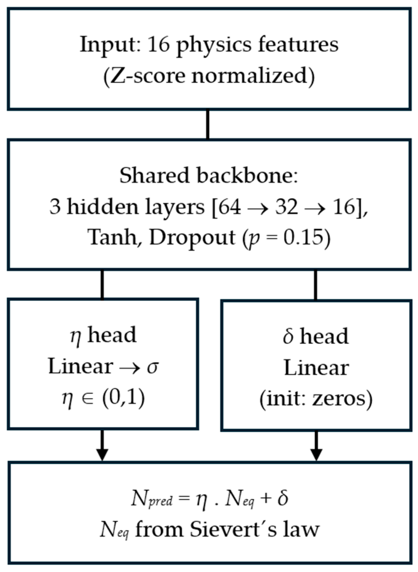
The physics-informed neural network architecture developed in this study, designated NitroPINN, employs a multiplicative structure that directly encodes the relationship between the actual nitrogen content in crude steel and its Sievert equilibrium value [28,29]. It is noted that the NitroPINN architecture does not employ ordinary or partial differential equation residuals evaluated at collocation points with automatic differentiation, which is the defining characteristic of the original PINN formulation by Raissi et al. [28]. Instead, the present model belongs to the category of physics-constrained or physics-guided neural networks within the broader taxonomy of physics-informed machine learning established by Karniadakis et al. [29], who explicitly identified three complementary modes of physics infusion: (a) physics-based preprocessing and feature engineering, (b) innovative network architectures that encode physical structure, and (c) physics-regularized loss functions. The NitroPINN architecture simultaneously employs all three of these modes: physics-derived features (N_eq, f_N, 1 – θ, C_rate) are constructed from first principles (Section 2.2); the multiplicative η·N_eq structure encodes the sub-equilibrium physics of the BOF directly into the prediction equation; and the composite loss function penalizes η values outside metallurgically plausible bounds. The term ‘physics-informed’ is therefore used in the present manuscript in accordance with this broader definition, and the model’s name NitroPINN is retained to reflect this multi-modal physics infusion. The physics penalty loss component constraining η to metallurgically plausible bounds is conceptually analogous to the compatibility loss enforced in sequential bc-PINN training schemes [34,35], where physical consistency across solution segments is preserved through dedicated loss terms rather than through differential equation residuals. The central prediction equation to predicting the nitrogen content in crude steel prior to tapping from the BOF vessel takes the form (11).

$$N_{pred}=\eta \left(x\right)·N_{eq}+\delta \left(x\right)$$

(11)

where x denotes the input feature vector (16 features after standardization), η(x) ∈ (0, 1) is a learned scalar representing the fraction of Sievert equilibrium achieved in the BOF bath, N_eq is the heat-specific equilibrium nitrogen content computed from thermodynamics (Section 2.2.1), and δ(x) is a small additive correction term. The physical motivation for this architecture is straightforward: in a top-blown BOF with intense CO boiling, the actual nitrogen content is invariably below the Sievert equilibrium value [13,17]. The multiplicative factor η directly encodes this sub-equilibrium behavior, constraining the prediction to a physically meaningful range without requiring the network to learn the equilibrium relationship from data alone. It is acknowledged that the present model operates as a static end-point predictor; temporal integration of the nitrogen mass balance throughout the blowing period represents a natural extension, contingent on the availability of continuous in-blow process data.

The network backbone consists of three hidden layers with [64 → 32 → 16] neurons and hyperbolic tangent (Tanh) activation functions, with dropout regularization (p = 0.15) applied after each hidden layer. The Tanh activation was selected over the more commonly used ReLU for its smoothness and bounded output range, which promotes stable gradient propagation through the physics-constrained loss function. Two output heads branch from the shared backbone: (a) the η head, comprising a single linear layer followed by a sigmoid activation to constrain η ∈ (0, 1); and (b) the δ head, comprising a single linear layer with weights and bias initialized to zero, ensuring that the initial prediction defaults to (η·N_eq) with no additive correction. The complete NitroPINN architecture is schematically illustrated in Figure 1.

The composite loss function (L) is computed based on Equation (12), where L_data = MSE (N_pred, N_final) is the standard mean squared error between the predicted and measured nitrogen values. For the purposes of loss computation, N_final was expressed in weight fraction (converted from ppm by division by 10⁶), consistent with the Sievert’s law formulation in which the nitrogen concentration is expressed in wt%; ppm values are used exclusively for reporting and interpretability throughout the manuscript. The AdamW optimizer with adaptive moment estimation further mitigates gradient scaling issues arising from the small absolute magnitude of the target variable. L_physics is calculated based on Equation (13), where n is the number of samples. L_physics penalizes extreme η_i values outside the physically plausible range, reflecting the metallurgical expectation that the equilibrium attainment fraction should lie between 5% and 95%. The bounds of 0.05 and 0.95 were selected as deliberately conservative safety limits, designed to prevent the sigmoid-constrained η output from collapsing towards the physically impossible extremes of zero or unity. In light of the post hoc observed η distribution (mean 0.456 ± 0.028, range 0.388–0.506), these bounds could be tightened—for example, to [0.10, 0.60]—in future work to more strongly constrain the model within the metallurgically plausible zone; the current broad limits were intentionally conservative to avoid imposing prior assumptions before the data distribution was known. L_delta (Equation (14)) is an L₂ regularization term that keeps the additive correction small, thereby preserving the physical interpretability of the multiplicative η·N_eq term.

$$L=L_{data}+\left({\lambda }_{phys}·L_{physics}\right)+\left({\lambda }_{req}·L_{delta}\right)$$

(12)

$$L_{physics}={\displaystyle \frac{1}{n}}{\displaystyle \sum _{i=1}^n}\left[ReLU{\left({\eta }_i-0.95\right)}^2+ReLU{\left(0.05-{\eta }_i\right)}^2\right]$$

(13)

$$L_{delta}={\displaystyle \frac{1}{n}}{\displaystyle \sum _{i=1}^n}{\delta }_i^2$$

(14)

The loss weights were set to λ_phys = 0.05 and λ_reg = 0.01 based on preliminary hyperparameter exploration.

Training employed the AdamW optimizer with an initial learning rate of 2 × 10⁻³ and weight decay of 10⁻³. A CosineAnnealingWarmRestarts learning rate scheduler (T₀ = 500, T_mult = 2, η_min = 10⁻⁶) was employed to facilitate escape from local minima in the non-convex loss landscape. Gradient clipping with a maximum norm of 1.0 was applied to prevent gradient explosion. Early stopping with a patience of 600 epochs and a maximum of 5000 epochs was used to prevent overfitting.

2.4. Baseline Models

Two baseline models were implemented for comparative benchmarking, both operating on the identical set of 16 physics-based features described in Section 2.2.

Ridge Regression: An L₂-regularized linear regression model was fitted using scikit-learn, with the regularization hyperparameter α selected from the candidate set {0.001, 0.01, 0.1, 1.0, 10.0, 100.0} based on validation performance within each cross-validation fold. Ridge regression serves as a robust linear baseline that is resistant to multicollinearity among the physics-based features.

Pure MLP: A multilayer perceptron with the same backbone architecture as the PINN (three hidden layers with [64 → 32 → 16] neurons) was trained using SiLU (Sigmoid Linear Unit) activation functions and dropout (p = 0.15). The MLP employed the same training configuration (AdamW optimizer, learning rate schedule, gradient clipping, early stopping) as the PINN but without any physics-based loss components and without the multiplicative N_eq structure—the output was a direct regression from the backbone to a single scalar value. This architecture isolates the contribution of the physics-informed components by providing a matched non-linear baseline.

2.5. Evaluation Protocol

Model performance was evaluated using 5-fold cross-validation (KFold with shuffle = True, random_state = 42), ensuring that each of the 66 heats appeared in exactly one validation fold. Within each fold, input features were standardized using z-score normalization (scikit-learn StandardScaler) fitted on the training partition and applied to the validation partition, thereby preventing information leakage. All three models (ridge regression, MLP, and NitroPINN) were evaluated on identical fold splits to ensure a fair comparison. Four complementary metrics were computed from the pooled out-of-fold predictions, all expressed in the original ppm scale: root mean squared error (RMSE), mean absolute error (MAE), coefficient of determination (R²), and mean absolute percentage error (MAPE). The RMSE emphasizes large prediction errors, MAE provides a scale-interpretable average error magnitude, R² quantifies the proportion of target variance explained by the model, and MAPE expresses the prediction accuracy as a percentage of the measured value.

2.6. Software

All models were implemented in Python 3.14 using PyTorch 2.10 for the NitroPINN and MLP architectures and scikit-learn 1.8.0 for ridge regression. Data manipulation was performed with pandas 3.0.2 and NumPy 2.4.4. Feature standardization used the StandardScaler 1.8.0 from scikit-learn 0.22, and matplotlib 3.10.8 was employed for data visualization. Z-score normalization (zero mean, unit variance) was applied to all input features.

3. Results

3.1. Data Matching and Exploratory Analysis

The heat-matching procedure successfully linked all 66 BOF heats with their corresponding desulfurized pig iron records, with the maximum weight difference between matched pairs being 400 kg. Although all models were calculated for nitrogen content in [%] terms, numerical values related to nitrogen are presented in [ppm] for better readability and in accordance with metallurgical practice, unless otherwise specified.

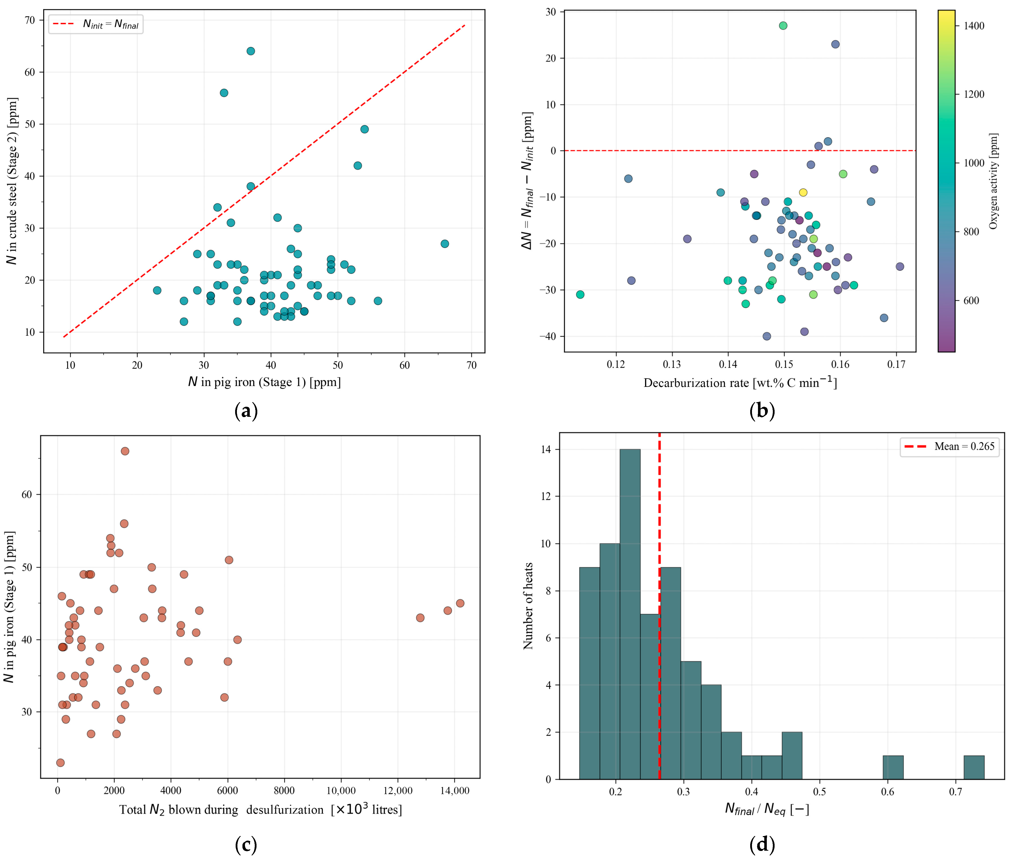
The initial nitrogen content (Stage 1) from desulfurized pig iron (N_init) ranged from 23 to 66 ppm with a mean of approximately 40 ppm. The target variable (Stage 2), nitrogen content in crude steel (N_final), ranged from 12 to 64 ppm with a mean of approximately 25 ppm. The computed Sievert equilibrium nitrogen content (N_eq) ranged from 66 to 107 ppm across the 66 heats.

The nitrogen change during BOF blowing, defined as ΔN = N_final – N_init, ranged from −40 to +27 ppm. The majority of heats exhibited ΔN < 0, indicating net nitrogen removal during oxygen blowing, which is consistent with the expected effect of CO flushing during vigorous decarburization [45,46]. The observed equilibrium attainment ratio, defined as N_final/N_eq, averaged 0.265 across all heats, confirming that the BOF bath reaches only approximately 27% of the Sievert equilibrium nitrogen content under the real operating conditions. This substantial departure from equilibrium is attributed to the combined effects of low nitrogen partial pressure in the converter atmosphere, surface blockage by dissolved oxygen and sulfur, and intense nitrogen stripping by CO bubbles [15]. Exploratory analysis of the nitrogen behavior is illustrated in Figure 2a–d.

3.2. Benchmark Results

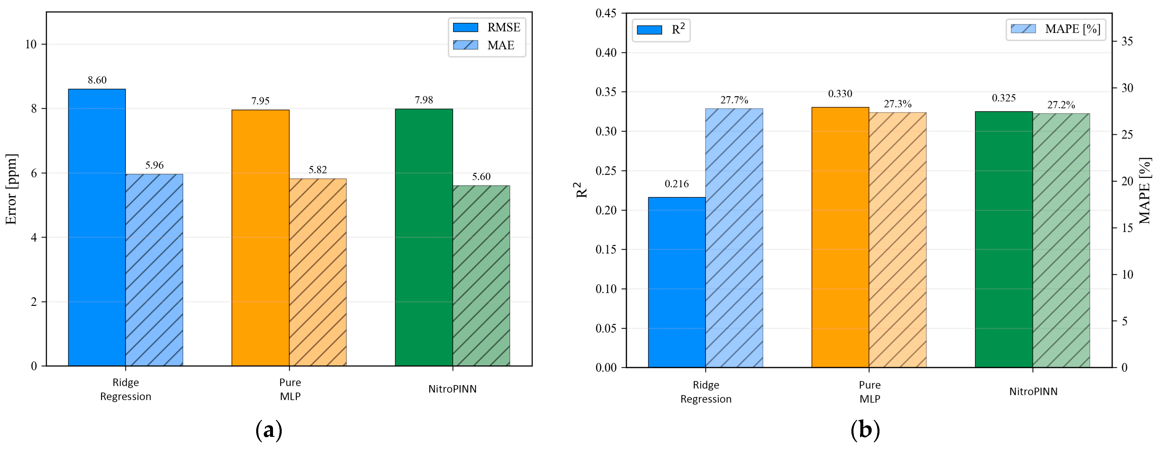
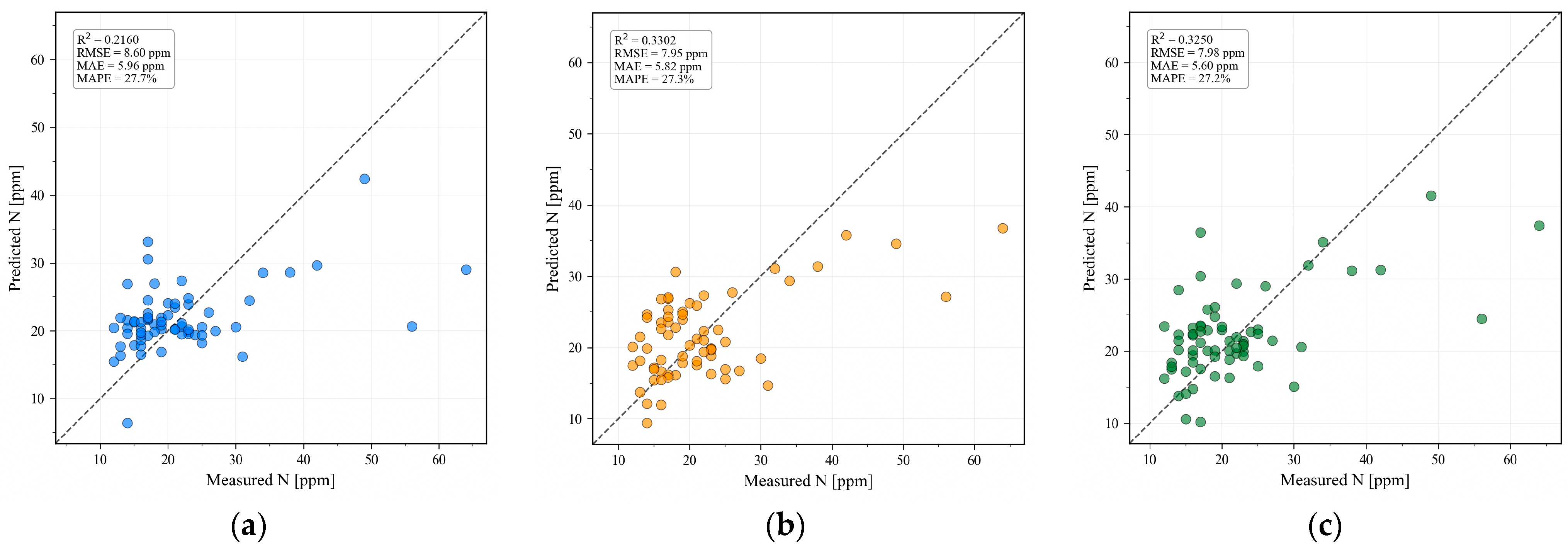
The pooled five-fold cross-validation results for the three models are summarized in

Table 3. Pooled five-fold cross-validation results for nitrogen prediction in crude steel.

Model	RMSE [ppm]	MAE [ppm]	R2	MAPE [%]	100 – MAPE [%]
Ridge Regression	8.60	5.96	0.216	27.7	72.3
Pure MLP	7.95	5.82	0.330	27.3	72.7
NitroPINN	7.98	5.60	0.325	27.2	72.8

. The NitroPINN achieved the lowest MAE (5.60 ppm) and MAPE (27.2%) among the three models; however, the differences relative to the Pure MLP are marginal and statistically inconclusive at n = 66—the pure MLP achieves a marginally superior RMSE (7.95 vs. 7.98 ppm) and R² (0.330 vs. 0.325), and the absolute MAE advantage of the NitroPINN amounts to 0.22 ppm. All three models should therefore be considered broadly comparable in terms of predictive accuracy. The difference of 0.005 in R² between the MLP and NitroPINN lies well within the fold-to-fold variance demonstrated in Table 3 and is not statistically meaningful at this sample size; the principal advantage of the NitroPINN lies in its physical interpretability and metallurgically constrained prediction structure, consistent with the established rationale for physics-informed learning in data-scarce regimes. Ridge regression exhibited the highest MAE (5.96 ppm) and the lowest R² (0.216), consistent with its inability to capture non-linear relationships in the data. The NitroPINN predictions exhibit a tighter clustering around the parity line for heats in the 15–30 ppm range, which constitutes the majority of the dataset, whilst all three models show increased scatter for heats with nitrogen contents exceeding 40 ppm.

Figure 3a,b present a graphical comparison of the RMSE, MAE, R², and MAPE across the three models (ridge regression, pure MLP and NitroPINN).

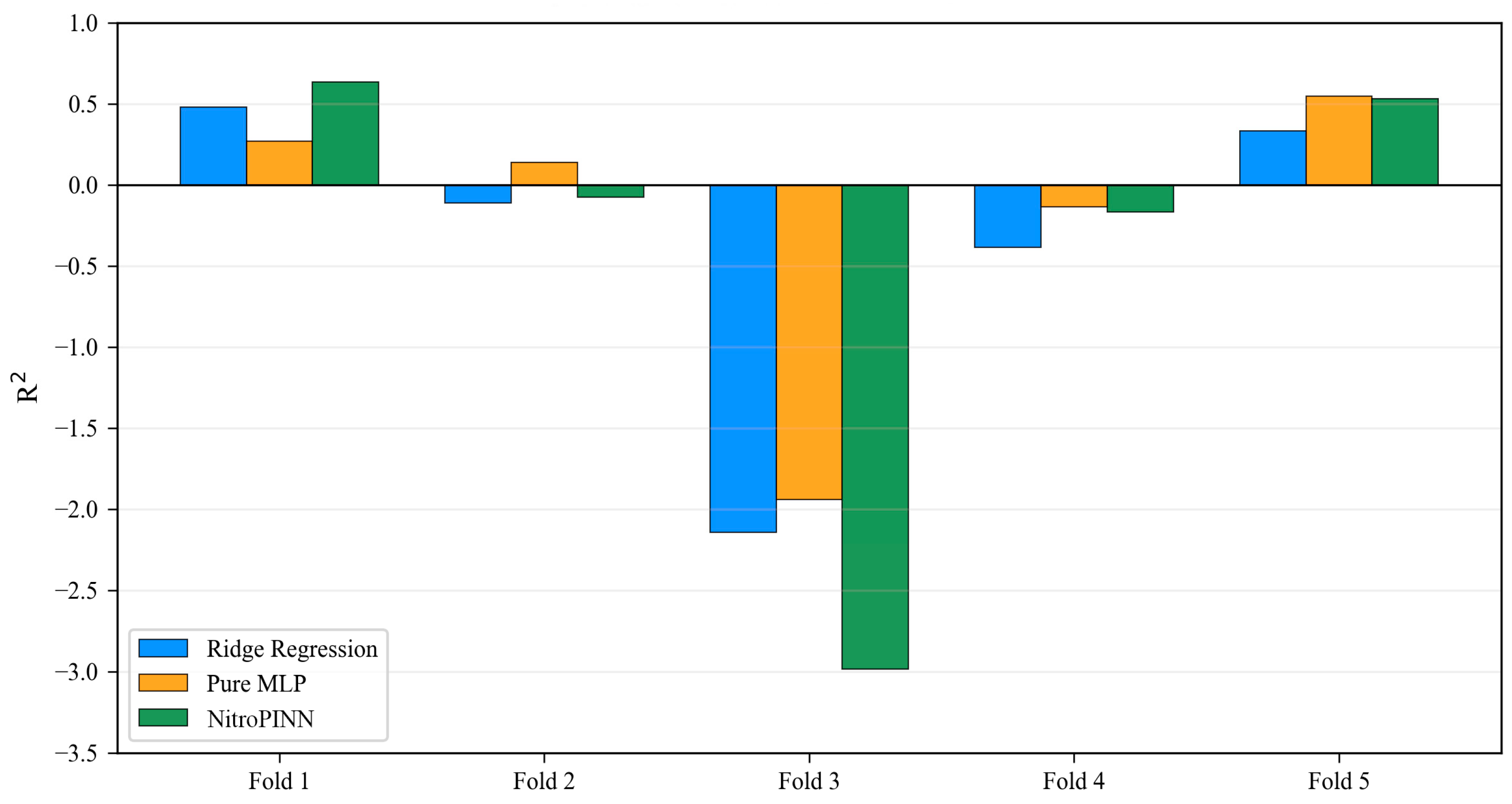
The per-fold results, presented in

Table 4. Per-fold R² values for the three models across five-fold cross-validation.

Fold	Ridge Regression R2	Pure MLP R2	NitroPINN R2
1	0.479	0.268	0.635
2	−0.113	0.136	−0.076
3	−2.143	−1.942	−2.984
4	−0.387	−0.137	−0.168
5	0.334	0.546	0.532

, reveal substantial fold-to-fold variability across all three models, which is attributable to the small sample size (~13 samples per validation fold). Notably, Fold 3 yielded negative R² values for all models (Ridge: −2.143, MLP: −1.942, PINN: −2.984), indicating that this particular fold contained heats with nitrogen behavior poorly represented by the training data. The occurrence of negative R² in Fold 3 across all three models—including the linear ridge regression baseline—confirms that this instability is a consequence of the small validation partition size and an unfavorable fold composition, rather than a model-specific deficiency; this behavior is a well-documented characteristic of small-sample cross-validation. Increasing the total dataset to ≥200 heats would substantially reduce fold-to-fold variance and eliminate such artefacts. Conversely, Fold 1 produced the highest R² for the NitroPINN (0.635), demonstrating strong predictive capability when the validation heats are well-covered by the training distribution. A graphical representation of the per-fold R² distribution is shown in Figure 4.

The parity plots of the measured versus predicted nitrogen content for all three models are presented in Figure 5a–c. The NitroPINN predictions exhibit a tighter clustering around the parity line for heats in the 15–30 ppm range, which constitutes the majority of the dataset, whilst all three models show increased scatter for heats with nitrogen contents exceeding 40 ppm.

3.3. NitroPINN Physics Parameters

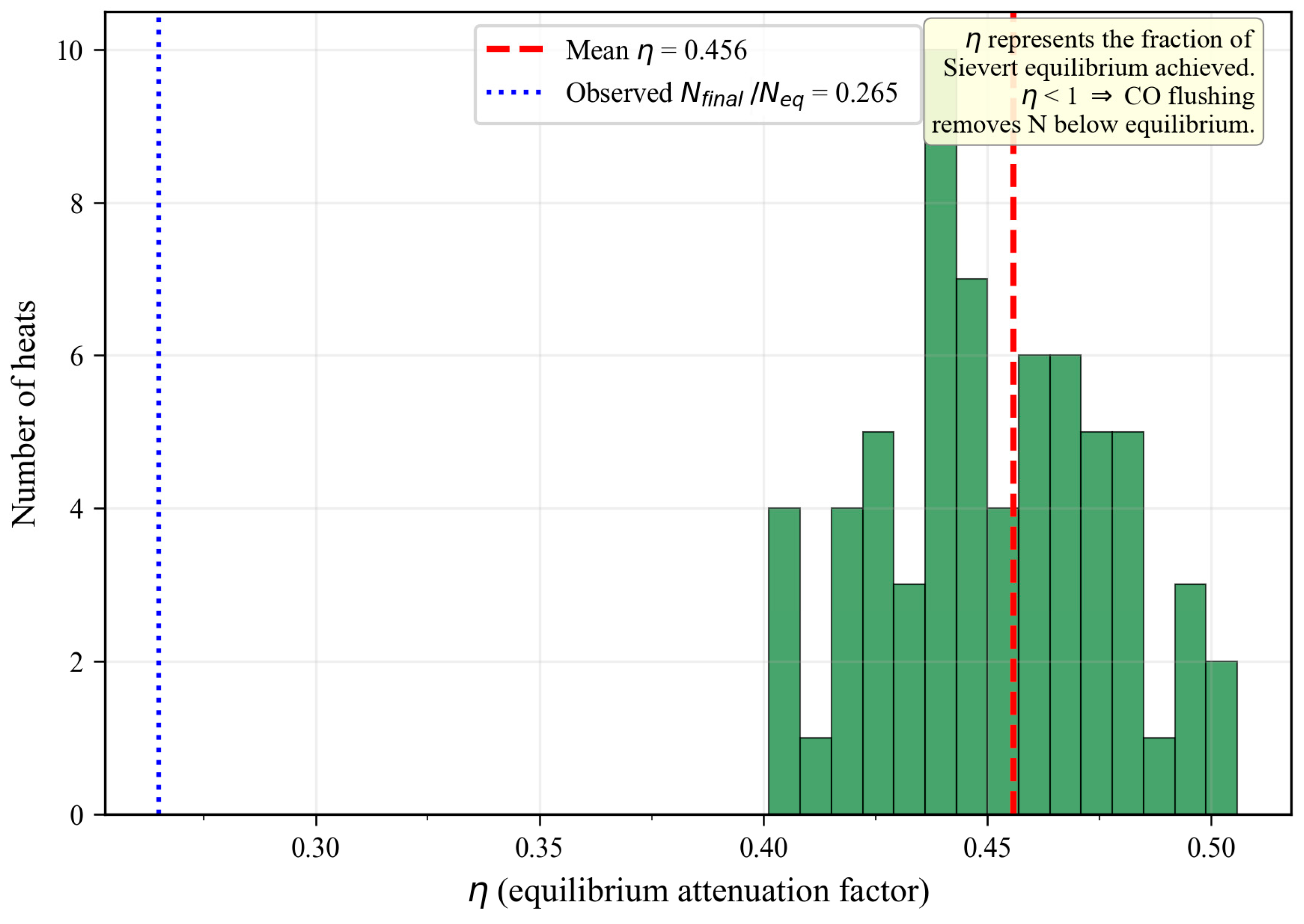
The η parameter learned by the NitroPINN model provides direct physical insight into the degree of equilibrium attainment in the BOF. Across all 66 heats and all cross-validation folds, the mean η value was 0.456 ± 0.028 (standard deviation), with a range of [0.388, 0.506]. This remarkably tight distribution indicates that the PINN consistently estimates the BOF bath to achieve approximately 46% of the Sievert equilibrium nitrogen content, with relatively little variation across heats despite differences in operating conditions (blowing time, scrap ratio, tapping temperature, and reblow occurrence). The η distribution is shown in Figure 6. The parameter η represents the fraction of Sievert equilibrium achieved in the BOF bath; values η < 1 are physically consistent with the sub-equilibrium nitrogen content imposed by intensive CO flushing during oxygen blowing.

The δ correction term remained small across all predictions, with a mean absolute value of approximately 2–3 ppm, confirming that the multiplicative η·N_eq component captures the dominant physics whilst δ provides fine-tuning adjustments for heat-specific deviations. The combined prediction η·N_eq + δ correctly targets the sub-equilibrium range observed in the raw data (mean N_final/N_eq = 0.265), with the discrepancy between η ≈ 0.46 and the observed ratio ≈ 0.27 being reconciled by the typically negative δ correction.

4. Discussion

4.1. Comparison with Previous Work

The present results may be contextualized by comparison with two prior studies conducted by the same research group on overlapping industrial datasets. Demeter et al. [39] benchmarked eight conventional ML models for nitrogen prediction at four BOF steelmaking stages using an 80/20 train–test split with 32 raw features. For the prediction of nitrogen in molten crude steel prior to tapping from the BOF vessel, the best-performing model was a feedforward neural network (FNN) with a reported accuracy of 79.77% (corresponding to a MAPE = 20.23%) and R² = 0.84, whilst ridge regression achieved 65.59% accuracy. Demeter et al. [40] subsequently applied AutoML (Microsoft Azure) to the same dataset, confirming the superiority of the ensemble architectures (MAPE = 20.64%).

The present PINN study differs from these prior works in several important respects. Firstly, the feature set has been reduced from 32 raw parameters to 16 physics-informed features, which sacrifices some information content in favor of physical interpretability and regularization. Secondly, the evaluation protocol employs five-fold cross-validation rather than a single 80/20 split, yielding more conservative and statistically robust estimates of generalization performance. The NitroPINN MAPE of 27.2% is therefore not directly comparable with the 20.23% reported in [39], as the two studies differ in feature set (16 physics-informed vs. 32 raw features), dataset composition, and evaluation protocol (five-fold CV vs. single 80/20 split). No claim of cross-study model superiority is made; the present benchmarking is strictly confined to the three models evaluated under identical conditions on the current 66-heat dataset. A rigorous cross-protocol comparison—in which the models from would be re-evaluated on the present dataset under the same five-fold CV scheme—was not conducted in this study, as the structural difference in feature sets renders such a comparison inherently confounded. It is further acknowledged that the marginal quantitative differences between the NitroPINN and the pure MLP (ΔMAE = 0.22 ppm, ΔMAPE = 0.1 percentage points) do not constitute evidence of predictive superiority; the primary contribution of the physics-constrained architecture is the interpretability of the learned η parameter and the thermodynamically grounded prediction structure, rather than incremental accuracy gains over a matched data-driven baseline. The identification of physically meaningful parameters from limited industrial data—here, the equilibrium attainment factor η—is consistent with the inverse analysis capabilities demonstrated for physics-informed architectures in other engineering domains, including geotechnical parameter recovery from noisy consolidation observations [36].

4.2. Physical Interpretability of the η Parameter

The mean η ≈ 0.46 learned by the NitroPINN indicates that the BOF bath achieves roughly 46% of the thermodynamic equilibrium nitrogen content predicted by Sievert’s law. This value carries direct metallurgical significance. During the approximately 17 min oxygen blow, the carbon content of the melt decreases from approximately 4.4% (pig iron) to 0.03–0.07% (crude steel), generating an enormous volume of CO gas that rises through the bath and strips dissolved nitrogen by physical entrainment and mass transfer across the bubble surfaces. The vigorous CO boiling creates conditions far from equilibrium with respect to nitrogen, as the effective p_N2 is exceedingly low and the contact time between the gas and liquid phases is limited by the rapid rise in velocity of CO bubbles.

The observed ratio N_final/N_eq from the raw data averages 0.265 (27%), which is lower than the PINN’s η ≈ 0.46. This apparent discrepancy is physically meaningful and arises because the PINN’s δ correction is typically negative (mean δ ≈ −2 to −3 ppm). The combined prediction η·N_eq + δ thus correctly targets the observed sub-equilibrium range. The separation of the prediction into a multiplicative thermodynamic component (η·N_eq) and an additive kinetic correction (δ) provides a physically transparent decomposition: the former captures the equilibrium-driven upper bound modulated by the degree of CO flushing, whilst the latter accommodates heat-specific deviations arising from variations in scrap quality, reblow occurrence, or slag chemistry.

The narrow range of η values (0.388–0.506, standard deviation 0.028) across all heats and folds indicates that the degree of equilibrium attainment is remarkably consistent under the standard operating conditions of the 170-ton BOF converter. This consistency reflects the standardized blowing practice: the oxygen flow rate, lance height profile, and blow duration are controlled within tight operational windows for each steel grade, resulting in similar CO evolution patterns and hence similar nitrogen stripping efficiencies across heats.

4.3. Role of N_init from Pig Iron Desulfurization

The incorporation of N_init from desulfurized pig iron as a predictive feature for BOF nitrogen content constitutes a novel contribution of the present study. The physical rationale is that the nitrogen content of the pig iron charged into the BOF establishes the initial boundary condition for the nitrogen mass balance during oxygen blowing [5,22]. The ΔN analysis (Section 3.1) demonstrated that the majority of heats exhibit net nitrogen removal during BOF blowing (ΔN < 0), with the extent of removal correlating with the initial nitrogen level, the decarburization rate, and the surface blockage parameter. Heats with higher N_init values tend to experience larger absolute nitrogen losses, which is consistent with the thermodynamic driving force for denitrogenating being proportional to the saturation (N_final – N_eq) [47].

The link between the desulfurization practice and final nitrogen content is mediated by the N₂ carrier gas used during the injection of the Mg + CaO desulfurization mixture. The total volume of N₂ blown during desulfurization directly contributes to nitrogen pickup in the pig iron, which then carries over into the BOF as the initial nitrogen content. This cross-stage coupling—wherein an upstream process parameter (desulfurization N₂ blow) influences the downstream prediction target (BOF nitrogen)—is precisely the type of process chain interaction that purely stage-isolated models cannot capture.

4.4. Limitations and Future Work

Although the raw data were carefully processed, it is important to note that these are industrial data from the steel production process in an oxygen converter, characterized by a high degree of non-linearity. The performance of the Nitro-PINN model is determined by the size of the dataset. With approximately 13 samples per validation fold, all three models exhibit high fold-to-fold variance, with some folds producing negative R² values (Table 4). This instability is a well-documented consequence of small-sample machine learning, where the composition of individual folds can disproportionately influence performance estimates [31]. The PINN architecture partially mitigates this issue by constraining predictions to physically plausible ranges through the embedded Sievert’s law and the bounded η parameter, but the limited data volume remains insufficient for the neural network components (η and δ heads) to learn fine-grained patterns across the full operating space.

Several additional limitations warrant discussion. The estimated partial pressure of nitrogen (p_{N2_est}) is a proxy derived from gas-phase composition estimates rather than direct off-gas measurement. Real-time off-gas analysis, which is available in some modern BOF installations but was not implemented during the present sampling campaign, would provide a substantially more accurate nitrogen partial pressure and thereby improve the quality of the N_eq computation. Similarly, the temperature and carbon content during the blow are not measured continuously—only end-of-blow values are available. Temporal profiles of temperature and carbon would enable the construction of a true kinetic PINN with ordinary differential equation (ODE) integration, modeling the time evolution of nitrogen throughout the blowing period rather than predicting only the end-point value.

The dataset of 66 heats was the maximum achievable within the constraints of the dedicated sampling campaign conducted between 17 and 22 May 2025. The cost of combustion analysis (ELTRA ON-900, certified reference materials, duplicate measurements in accordance with ASTM E-1019) imposed a significant financial burden on the project budget, and the requirement to match each BOF heat with its corresponding desulfurized pig iron record (Stage 1) further restricted the sample to heats for which both records were available and could be reliably linked. Ongoing collaboration with the industrial partner U. S. Steel Košice is planned to expand the dataset to a minimum of 200 matched heats, which would provide the statistical power required for robust generalization. The cost of laboratory analysis of the samples placed a significant burden on the limited project budget, which affected the size of the data sample analyzed. However, subsequent collaboration with an industrial partner will enable us to analyze a larger dataset. Nevertheless, this article presents a methodology and procedure for evaluating a model based on a PINN. Future research plans to cover a wider range of steel grades and scrap ratios. This will provide sufficient statistical power for robust five- or 10-fold cross-validation. Implementing k-fold cross-validation stratified by steel grade would further improve the representativeness of each fold. Integrating temporal blowing data (for example, off-gas analysis) would allow us to develop a dynamic PINN with time-dependent η(t) and δ(t) functions. This would capture the evolution of equilibrium attainment throughout the blow, rather than modeling it as a single end-point value.

5. Conclusions

This study developed and validated a physics-constrained neural network (NitroPINN) with a novel multiplicative η architecture, embedding physical knowledge through thermodynamic feature engineering, a multiplicative prediction structure, and a physics-penalizing composite loss function for predicting nitrogen content in crude steel before tapping from a top-blown basic oxygen furnace. The NitroPINN embeds Sievert’s law equilibrium, Wagner interaction coefficients, and Byrne–Belton surface blockage theory directly into its prediction mechanism through the formulation N_pred = η(x)·N_eq + δ(x), achieving competitive prediction accuracy (MAE = 5.60 ppm, MAPE = 27.2%, R² = 0.325) under rigorous five-fold cross-validation on 66 matched industrial heats from steel producer. The learned η parameter, averaging 0.456 ± 0.028, quantifies the degree of Sievert equilibrium attainment in the BOF bath and is consistent with the expected sub-equilibrium conditions arising from intense CO flushing during oxygen blowing. All three benchmarked models (ridge regression, MLP, and NitroPINN) exhibited comparable overall accuracy, confirming that dataset size rather than model architecture constitutes the current bottleneck for prediction improvement. The primary advantage of the NitroPINN physics-informed machine learning approach lies in its physical interpretability, which constrains predictions to metallurgically plausible ranges and provides transparent decomposition into equilibrium and kinetic contributions. Future work will expand the dataset to at least 200 heats and incorporate temporal blowing profiles to enable dynamic physics-informed modeling of nitrogen evolution throughout the BOF process.

References

1. Mahanta, B.K.; Gupta, P.; Mohanty, I.; Roy, T.K.; Chakraborti, N. Evolutionary Data Driven Modeling and Tri-Objective Optimization for Noisy BOF Steel Making Data. Digit. Chem. Eng. 2023, 7, 100094. [Google Scholar] [CrossRef]
2. Zhao, F.; Liu, X.; Zhang, Z.; Xie, J. Effect of Nitrogen Content on the Mechanical Properties and Deformation Behaviors of Ferritic-Pearlitic Steels. Mater. Sci. Eng. A 2022, 855, 143918. [Google Scholar] [CrossRef]
3. Hänninen, H.; Romu, J.; Ilola, R.; Tervo, J.; Laitinen, A. Effects of Processing and Manufacturing of High Nitrogen-Containing Stainless Steels on Their Mechanical, Corrosion and Wear Properties. J. Mater. Process. Technol. 2001, 117, 424–430. [Google Scholar] [CrossRef]
4. Bazaleeva, K.O. Mechanisms of the Influence of Nitrogen on the Structure and Properties of Steels (A Review). Met. Sci. Heat Treat. 2005, 47, 455–461. [Google Scholar] [CrossRef]
5. Misra, S.; Fruehan, R.J. Hydrogen and Nitrogen Control in Ladle and Casting Operations; Carnegie Mellon University Pittsburgh: Pittsburgh, PA, USA, 2005. [Google Scholar]
6. Turkdogan, E.T. Fundamentals of Steelmaking; Institute of Materials: London, UK, 2010. [Google Scholar]
7. Shamsuddin, M. Secondary Steelmaking. In Physical Chemistry of Metallurgical Processes, 2nd ed.; Springer International Publishing: Cham, Switzerland, 2021; pp. 293–351. [Google Scholar]
8. Slater, C.; Spooner, S.; Davis, C.; Sridhar, S. Observation of the Reversible Stabilisation of Liquid Phase Iron during Nitriding. Mater. Lett. 2016, 173, 98–101. [Google Scholar] [CrossRef]
9. Siwka, J. Equilibrium Constants and Nitrogen Activity in Liquid Metals and Iron Alloys. ISIJ Int. 2008, 48, 385–394. [Google Scholar] [CrossRef][Green Version]
10. Satir, A.; Feichtinger, H. On the Solubility of Nitrogen in Liquid Iron and Steel Alloys Using Elevated Pressure. Z. Fuer Met. 1991, 52, 689. [Google Scholar]
11. Jang, J.-M.; Kim, D.-H.; Paek, M.-K.; Pak, J.-J. Nitrogen Solubility in Cast Iron Containing C, Si and Mn. ISIJ Int. 2018, 58, 1185–1190. [Google Scholar] [CrossRef]
12. Jang, J.-M.; Seo, S.-H.; Jiang, M.; Paek, M.-K.; Wang, X.; Pak, J.-J. Nitrogen Solubility in Liquid Fe–C Alloys. ISIJ Int. 2014, 54, 32–36. [Google Scholar] [CrossRef]
13. Fruehan, R.J.; Goldstein, D.; Sarma, B.; Story, S.R.; Glaws, P.C.; Pasewicz, H.U. Recent Advances in the Fundamentals of the Kinetics of Steelmaking Reactions. Metall. Mater. Trans. B 2000, 31, 891–898. [Google Scholar] [CrossRef]
14. Kobayashi, A.; Tsukihashi, F.; Sano, N. Kinetic Studies on the Dissolution of Nitrogen into Molten Iron by 14N-15N Isotope Exchange Reaction. ISIJ Int. 1993, 33, 1131–1135. [Google Scholar] [CrossRef]
15. Byrne, M.; Belton, G.R. Studies of the Interfacial Kinetics of the Reaction of Nitrogen with Liquid Iron by the 15N-14N Isotope Exchange Reaction. Metall. Trans. B 1983, 14, 441–449. [Google Scholar] [CrossRef]
16. Pitkälä, J.; Xia, J.; Jokilaakso, A. CFD Modeling of Nitrogen Dissolution into a Steel Bath During Gas Purging. In Proceedings of the Second International Conference on CFD in the Minerals and Process Industries, CSIRO, Melbourne, Australia, 6–8 December 1999; pp. 35–40. [Google Scholar]
17. Inomoto, T.; Kitamura, S.; Yano, M. Kinetic Study of the Nitrogen Removal Rate from Molten Steel (Normal Steel and 17 mass%Cr Steel) under CO Boiling or Argon Gas Injection. ISIJ Int. 2015, 55, 1822–1827. [Google Scholar] [CrossRef]
18. Trotter, D.; Varcoe, D.; Reeves, R.; Hornby, S. Use of HBI and DRI for Nitrogen Control in Steel Products. SEAISI Q. 2002, 31, 39–50. [Google Scholar]
19. Patra, S.; Nayak, J.; Singhal, L.; Pal, S. Prediction of Nitrogen Content of Steel Melt during Stainless Steel Making Using AOD Converter. Steel Res. Int. 2017, 88, 1600271. [Google Scholar] [CrossRef]
20. Liu, C.; Tang, L.; Liu, J. A Stacked Autoencoder With Sparse Bayesian Regression for End-Point Prediction Problems in Steelmaking Process. IEEE Trans. Autom. Sci. Eng. 2020, 17, 550–561. [Google Scholar] [CrossRef]
21. Zhang, R.; Yang, J. State of the Art in Applications of Machine Learning in Steelmaking Process Modeling. Int. J. Miner. Metall. Mater. 2023, 30, 2055–2075. [Google Scholar] [CrossRef]
22. Nam, J.; Rout, B.; Chatterjee, S.; Van Ende, M.-A.; Jung, I.-H. Integrated Mathematical Model for Nitrogen Control in Oxygen Steelmaking Process. Metall. Mater. Trans. B 2025, 56, 2202–2223. [Google Scholar] [CrossRef]
23. Yoon, C.; Eom, C.; Jeon, Y.; Kim, K. Development of a Nitrogen Prediction Model for 320 Tonne Converter. In Proceedings of the 12th International Conference of Molten Slags, Fluxes and Salts (MOLTEN 2024) Proceedings, Brisbane, Australia, 17–19 June 2024. [Google Scholar] [CrossRef]
24. Li, B.; Li, C.; Jing, P.; Shi, C.; Wu, W.; Dong, K. Mechanism-Data Hybrid-Driven Modeling of Energy Consumption and Carbon Emission for Converter Steelmaking Process Optimization. J. Clean. Prod. 2025, 532, 146964. [Google Scholar] [CrossRef]
25. Liu, J.; Liu, H.; Chen, F.; Su, Y.; Li, H.; Xue, X. Dynamic Flame Feature-Driven Prediction Model for Basic Oxygen Furnace Steelmaking Endpoint Carbon Content Based on Three-Dimensional Multi-Layer Complex Networks. Eng. Appl. Artif. Intell. 2025, 139, 109564. [Google Scholar] [CrossRef]
26. Niu, D.; Hu, W.; Zhou, J.; Jia, M. Multi-Target Adversarial Transfer TabTransformer for BOF Endpoint Composition Prediction under Zero-Inflated Sparsity. Expert Syst. Appl. 2026, 322, 132349. [Google Scholar] [CrossRef]
27. Pawlik, L.; Wilk-Jakubowski, J.L.; Frej, D.; Wilk-Jakubowski, G. Applications of Computational Mechanics Methods Combined with Machine Learning and Neural Networks: A Systematic Review (2015–2025). Appl. Sci. 2025, 15, 10816. [Google Scholar] [CrossRef]
28. Raissi, M.; Perdikaris, P.; Karniadakis, G.E. Physics-Informed Neural Networks: A Deep Learning Framework for Solving Forward and Inverse Problems Involving Nonlinear Partial Differential Equations. J. Comput. Phys. 2019, 378, 686–707. [Google Scholar] [CrossRef]
29. Karniadakis, G.E.; Kevrekidis, I.G.; Lu, L.; Perdikaris, P.; Wang, S.; Yang, L. Physics-Informed Machine Learning. Nat. Rev. Phys. 2021, 3, 422–440. [Google Scholar] [CrossRef]
30. Cai, S.; Mao, Z.; Wang, Z.; Yin, M.; Karniadakis, G.E. Physics-Informed Neural Networks (PINNs) for Fluid Mechanics: A Review. Acta Mech. Sin. 2021, 37, 1727–1738. [Google Scholar] [CrossRef]
31. Cuomo, S.; Di Cola, V.S.; Giampaolo, F.; Rozza, G.; Raissi, M.; Piccialli, F. Scientific Machine Learning Through Physics–Informed Neural Networks: Where We Are and What’s Next. J. Sci. Comput. 2022, 92, 88. [Google Scholar] [CrossRef]
32. Lee, J.; Shin, S.; Kim, T.; Park, B.; Choi, H.; Lee, A.; Choi, M.; Lee, S. Physics Informed Neural Networks for Fluid Flow Analysis with Repetitive Parameter Initialization. Sci. Rep. 2025, 15, 16740. [Google Scholar] [CrossRef] [PubMed]
33. Badora, M.; Bartosik, P.; Graziano, A.; Szolc, T. Using Physics-Informed Neural Networks with Small Datasets to Predict the Length of Gas Turbine Nozzle Cracks. Adv. Eng. Inform. 2023, 58, 102232. [Google Scholar] [CrossRef]
34. Mattey, R.; Ghosh, S. A Novel Sequential Method to Train Physics Informed Neural Networks for Allen Cahn and Cahn Hilliard Equations. Comput. Methods Appl. Mech. Eng. 2022, 390, 114474. [Google Scholar] [CrossRef]
35. Lin, S.; Chen, Y. The Improved Backward Compatible Physics-Informed Neural Networks for Reducing Error Accumulation and Applications in Data-Driven Higher-Order Rogue Waves. Chaos Interdiscip. J. Nonlinear Sci. 2024, 34, 033139. [Google Scholar] [CrossRef]
36. Li, D.; Cao, Y.; Huang, S.; Cui, Y.; Wei, X.; Cao, H.; Wang, C. Lagged Backward-Compatible Physics-Informed Neural Networks for Unsaturated Soil Consolidation Analysis. Can. Geotech. J. 2026, 63, 1–28. [Google Scholar] [CrossRef]
37. Sun, Y.; Zhang, Q.; Raffoul, S. Physics-Informed Neural Network for Predicting Hot-Rolled Steel Temperatures during Heating Process. J. Eng. Res. 2025, 13, 1496–1504. [Google Scholar] [CrossRef]
38. Xia, Y.; Wang, H.; Xu, A. dmPINNs: An Integrated Data-Driven and Mechanism-Based Method for Endpoint Carbon Prediction in BOF. Metals 2024, 14, 926. [Google Scholar] [CrossRef]
39. Demeter, J.; Buľko, B.; Hrubovčáková, M. Predictive Modelling of Nitrogen Content in Molten Metal During BOF Steelmaking Processes via Python-Based Machine Learning: A Benchmarking of Statistical Techniques. Appl. Sci. 2026, 16, 3774. [Google Scholar] [CrossRef]
40. Demeter, J.; Buľko, B.; Demeter, P.; Hrubovčáková, M.; Hubatka, S.; Fogaraš, L. Automated Machine Learning for Nitrogen Content Prediction in Steel Production: A Comprehensive Multi-Stage Process Analysis. Appl. Sci. 2025, 16, 441. [Google Scholar] [CrossRef]
41. ASTM E1019-18; Standard Test Methods for Determination of Carbon, Sulfur, Nitrogen, and Oxygen in Steel, Iron, Nickel, and Cobalt Alloys by Various Combustion and Inert Gas Fusion Techniques. ASTM International: West Conshohocken, PA, USA, 2018. Available online: https://store.astm.org/e1019-18.html (accessed on 21 April 2026).
42. ELTRA GmbH. Basic Application Information. Available online: https://www.eltra.com/files/446383/expert-guide-application-information.pdf (accessed on 22 April 2026).
43. ELTRA GmbH. Effective Quality Control of Steel and Iron Products with Combustion Analysis. Available online: https://www.eltra.com/files/14146/effective-quality-control-of-steel-and-iron-products-with-combustion-analysis.pdf (accessed on 22 April 2026).
44. Seetharaman, S. Fundamentals of Metallurgy; CRC Press: Boca Raton, FL, USA, 2005. [Google Scholar]
45. Mukherjee, D.; Shukla, A.K.; Senk, D.G. Prediction of Decarburisation Process along with Hydrogen and Nitrogen Removal by Mathematical Modelling of RH Degassing Process. Ironmak. Steelmak. 2018, 45, 412–419. [Google Scholar] [CrossRef]
46. Lee, M.S.; Trimble, D.J.; Wibberley, L.J. Evaluation of Low-Grade Iron Carbide as a Reagent for Enhanced Nitrogen Desorption in Steel Melts. Scand. J. Metall. 2001, 30, 121–126. [Google Scholar] [CrossRef]
47. Zhang, Y.; Liu, J.; Yang, H.; Li, W.; Zhang, S.; Zhou, W. Kinetics of Nitrogen Absorption/Vacuum Denitrigenization and Precipitation Behavior of Nitrogen Bubbles in 42CrMoA Molten Steel. Steel Res. Int. 2025, 96, 2400071. [Google Scholar] [CrossRef]
Figure 1. Structure of the NitroPINN model architecture.
Applsci 16 05731 g001
Figure 2. Exploratory analysis of nitrogen behavior across steel production in BOF: (a) Ninit vs. Nfinal scatter plot; (b) nitrogen change ΔN = NfinalNinit as a function of decarburization rate, color-coded by oxygen activity [ppm]; the dashed red line denotes ΔN = 0; (c) Ninit as a function of total N2 volume blown during desulfurization; (d) histogram of the equilibrium attainment ratio Nfinal/Neq, (dashed red line denotes mean).
Applsci 16 05731 g002
Figure 3. Graphical comparison of RMSE, MAE, R2, and MAPE across the three predictive models: (a) RMSE and MAE comparison; (b) R2 and MAPE comparison.
Applsci 16 05731 g003
Figure 4. Per-fold R2 distribution across 5-fold cross-validation for three models.
Applsci 16 05731 g004
Figure 5. Parity plots of measured versus predicted nitrogen content in crude steel [ppm] for the three models evaluated under 5-fold cross-validation (n = 66 pooled out-of-fold predictions); the dashed line in each panel represents perfect prediction (predicted = measured): (a) ridge regression (R2 = 0.2160, RMSE = 8.60 ppm, MAE = 5.96 ppm, MAPE = 27.7%); (b) pure MLP (R2 = 0.3302, RMSE = 7.95 ppm, MAE = 5.82 ppm, MAPE = 27.3%); (c) NitroPINN (R2 = 0.3250, RMSE = 7.98 ppm, MAE = 5.60 ppm, MAPE = 27.2%).
Applsci 16 05731 g005
Figure 6. Distribution of the equilibrium attenuation factor η learned by the NitroPINN across all 66 heats and cross-validation folds. The red dashed line indicates the mean η = 0.456, and the blue dotted line indicates the observed raw data ratio NFINAL/Neq = 0.265 for reference.
Applsci 16 05731 g006