Comparison of Initialization Strategies for EM in High-Dimensional Multivariate Diagonal Gaussian Mixture Models

Abstract

Expectation Maximization (EM) iterations for Gaussian mixture models (GMMs) are highly sensitive to initial parameters, which calls for developing robust initialization methods. For multidimensional GMMs, the problem is even more severe than for univariate GMMs because of the larger number of parameters. For univariate or low-dimensional GMMs, several studies on their initialization have appeared in the literature, whereas research on initializing multivariate, high-dimensional GMMs remains limited. In this study, we compare several initializations for Multivariate Diagonal Gaussian Mixture Models (MDGMMs). In our study, we have included methods already used in the literature for initializing MDGMMs: Hierarchical Clustering, K-means, and random initialization. We have also used a new method, namely, Ensemble Clustering. A review of the existing literature suggests that Ensemble Clustering has not been used previously as an initialization strategy for MDGMM. Several metrics were used to evaluate the clustering quality. Our study demonstrates that Ensemble Clustering, while computationally intensive, is competitive with other methods for initializing MDGMMs.

1. Introduction

The rapid increase in dataset sizes and dimensions has posed a considerable challenge for researchers seeking to discover structures and extract knowledge from analyses using supervised and unsupervised approaches [1]. One example is the model-based, unsupervised clustering of high-dimensional data, where the model is the multidimensional mixture of probability distributions. In this approach, multivariate Gaussian mixture models (MGMMs) are most common for probability density approximation and clustering. MGMMs assume that the data points are generated from a mixture model, in which each component corresponds to a multivariate Gaussian distribution [2]. They offer flexibility not possible with simpler deterministic algorithms, specifically through soft probabilistic assignments and the ability to model clusters with varying shapes, sizes, and orientations. However, this flexibility comes at the expense of increased computational cost/complexity. The number of entries in the full covariance matrix increases quadratically with the number of variables/features. Algorithms used for their estimation in high-dimensional data are computationally expensive and can also be numerically unstable. Their results become less reliable and less informative, and clustering/classification performance may decrease [3].

To avoid overfitting and excessive computational complexity, parsimonious models are used [4]. A special case of this approach is the multivariate diagonal Gaussian mixture model (MDGMM), which comprises a mixture of multivariate Gaussian distributions with diagonal covariance matrices. Restricting the covariance matrix to a diagonal form allows for a drastic reduction in the number of estimated parameters. This approach allows fitting to data models of significantly larger size, which may yield better approximations of complex data distributions while maintaining numerical stability. The efficiency of the diagonal model, MDGMM, depends on the optimization process used to fit/calibrate the model to the dataset. Estimation of model parameters using the Expectation–Maximization (EM) algorithm [5,6] is an iterative method that does not guarantee convergence to a global optimum and may get stuck at a local one. Hence, the choice of a starting point (initialization method) strongly impacts the quality of the final model. Poor initialization can lead to “empty” clusters, slow convergence, or getting stuck in a suboptimal solution, which makes the entire analysis less reliable [7,8].

EM-based GMM fitting has been applied across various domains [9], and multiple studies have already examined its initialization methods. However, most previous studies on EM initialization for GMMs have focused either on univariate cases or on low-dimensional multivariate data [10,11]. Most previous studies on EM initialization for GMMs have focused either on univariate cases or on low-dimensional multivariate data. In the case of univariate models, the literature presents various initialization approaches such as random initialization and model-based methods [6,7,12], strategies based on quintiles or data clustering [13], or dynamic programming partitioning [14,15]. For multidimensional models, different initialization approaches have also been widely studied, including clustering-based strategies such as Hierarchical Clustering and K-means [16,17], as well as more advanced techniques based on singular value decomposition or EM trajectory properties [18,19]. However, while GMMs generally provide an accurate fit for standard data distributions [20], the number of dimensions considered in prior studies has typically remained limited and not truly high [21]. This limitation is important because a significant increase in dimensionality makes mixture estimation more difficult, both statistically and computationally [1,22]. Therefore, conclusions based on low- or moderate-dimensional data are less transferable to truly high-dimensional settings.

The main objective of this study is to evaluate and compare algorithms for initializing EM iterations in the MDGMM model for problems where the number of features in the dataset is large (at least hundreds). Compared algorithms for initialization are random, K-means clustering, Hierarchical Clustering, and Ensemble Clustering. Three of the above initialization methods, which we call standard initialization methods, random, K-Means Clustering, and Hierarchical Clustering, have already been applied in the literature. However, the fourth, Ensemble Clustering, is new as the initialization strategy for MDGMM. We verify the hypothesis that using the Ensemble Clustering method yields a statistically significant improvement in clustering quality compared to standard initialization methods (random, K-means, Hierarchical) in MDGMM.

2. Materials and Methods

The data matrix analyzed $\mathbf{X}$ has N observation vectors (columns), ${\mathbf{x}}_1,{\mathbf{x}}_2,\dots ,{\mathbf{x}}_N$,

$$\mathbf{X}=\left[{\mathbf{x}}_1,{\mathbf{x}}_2,\dots ,{\mathbf{x}}_N\right].$$

(1)

Each observation vector contains M entries (features) of continuous type,

$${\mathbf{x}}_n={\left[x_{n,1},x_{n,2},\dots ,x_{n,M}\right]}^T,$$

(2)

where $x_{n,m}$ is the m-th entry (feature) of the n-th observation vector. Observation vectors ${\mathbf{x}}_n$, assumed independent, are characterized by the model given by a mixture of Multivariate Diagonal Gaussian Distributions.

2.1. Multivariate Diagonal Gaussian Distribution

The Multivariate Diagonal Gaussian Distribution is the Multivariate Gaussian Distribution with a diagonal covariance matrix $\mathbf{\Sigma }$

$$\mathbf{\Sigma }=\left[\begin{array}{cccc}{\sigma }_1^2& 0& \cdots & 0\\ 0& {\sigma }_2^2& \cdots & 0\\ ⋮& ⋮& \ddots & ⋮\\ 0& 0& \cdots & {\sigma }_M^2,\end{array}\right]$$

(3)

so its probability density function $f(\mathbf{x},\mathit{\mu },\mathbf{\Sigma })$, with $\mathbf{\Sigma }$ above and

$$\mathbf{x}={\left[x_1,x_2,\dots x_M\right]}^T,\mathit{\mu }={\left[{\mathit{\mu }}_1,{\mathit{\mu }}_2,\dots ,{\mathit{\mu }}_M\right]}^T$$

(4)

is a product of univariate Gaussian probability density functions $f_m(x_m,{\mu }_m,{\sigma }_m)$,

$$f(\mathbf{x},\mathit{\mu },\mathbf{\Sigma })={\displaystyle \frac{1}{{\left(2\pi \right)}^{M/2}{\left|\mathbf{\Sigma }\right|}^{1/2}}}exp\left(-{\displaystyle \frac{1}{2}}{(\mathbf{x}-\mathit{\mu })}^T{\mathbf{\Sigma }}^{-1}(\mathbf{x}-\mathit{\mu })\right)={\displaystyle \prod _{m=1}^M}{f}_m(x_m,{\mu }_m,{\sigma }_m),$$

(5)

$$f_m(x_m,{\mu }_m,{\sigma }_m^2)={\displaystyle \frac{1}{\sqrt{2\pi {\sigma }_m^2}}}exp\left(-{\displaystyle \frac{{(x_m-{\mu }_m)}^2}{2{\sigma }_m^2}}\right).$$

(6)

Compared to the multivariate Gaussian distribution with a full covariance matrix, which has ${\displaystyle \frac{M(M+1)}{2}}$ covariance/variance parameters, the multivariate diagonal Gaussian distribution contains only M variances of the components of the observation vector. This is crucial for the computational efficiency of the EM algorithm and the stability of estimation in high-dimensional spaces.

2.2. Multivariate Diagonal Gaussian Mixture Model (MDGMM)

The mathematical model for dataset clustering, MDGMM, is a mixture of multivariate diagonal Gaussian distributions (5). Assuming K mixture components, introducing mixing proportions (also called component weights) ${\alpha }_1,{\alpha }_2,\dots ,{\alpha }_K$, ${\alpha }_1+{\alpha }_2+\dots +{\alpha }_K=1$ and using the index k for the parameters of the mixture components, one obtains the following expression for the probability density function of the MDGMM:

$$\begin{array}{c}\hfill f_{MDGMM}(\mathbf{x},{\alpha }_1,{\alpha }_2,\dots ,{\alpha }_K,{\mathit{\mu }}_1,{\mathit{\mu }}_2,\dots ,{\mathit{\mu }}_K,{\mathbf{\Sigma }}_1,{\mathbf{\Sigma }}_2,\dots ,{\mathbf{\Sigma }}_K)\end{array}$$

(7)

$$\begin{array}{c}\hfill ={\displaystyle \sum _{k=1}^K}{\alpha }_k{f}_k(\mathbf{x},{\mathit{\mu }}_{\mathit{k}},{\mathbf{\Sigma }}_{\mathit{k}})={\displaystyle \sum _{k=1}^K}{\alpha }_k{\displaystyle \prod _{m=1}^M}{f}_{k,m}(x_m,{\mu }_{k,m},{\sigma }_{k,m}),\end{array}$$

(8)

where

$$f_{k,m}(x_m,{\mu }_{k,m},{\sigma }_{k,m})={\displaystyle \frac{1}{\sqrt{2\pi }{\sigma }_{k,m}}}exp\left[-{\displaystyle \frac{1}{2}}{\left({\displaystyle \frac{x_m-{\mu }_{k,m}}{{\sigma }_{k,m}}}\right)}^2\right].$$

(9)

2.3. Likelihood Function of the Dataset

Assuming the MDGMM (8), the likelihood function of the dataset (2) is as follows:

$$L(x_1,x_2,\dots x_n,\dots ,x_N)={\displaystyle \prod _{n=1}^N}{\displaystyle \sum _{k=1}^K}{\alpha }_k{\displaystyle \prod _{m=1}^M}{f}_{k,m}(x_{n,m},{\mu }_{k,m},{\sigma }_{k,m})$$

(10)

2.4. EM Recursive Algorithm for Mixture Parameters Estimation

The main idea behind the EM algorithm is that there are hidden (latent) variables that are not directly observable. EM recursions alternate between two steps: expectation (E-step), in which the expected values of the latent variables are calculated from current parameter estimates given observed data, and maximization (M-step), in which the parameters are re-estimated based on the expected values of the latent variables from the E-step. These two steps are repeated until convergence is achieved. The hidden variables in the EM algorithm to estimate the parameters of the MDGMM (8) are scalars $z_1,z_2,\dots ,z_N$, which assign observation vectors (2) to the components of the mixture, $z_n=k$, if the observation vector $x_n$ was generated by the component k of the mixture. In other words $z_n=k$ if $x_n$ belongs to component k, and then we have

$$z_n=k\mathrm{if}\mathrm{observation}{\mathbf{x}}_n\mathrm{belongs}\mathrm{to}\mathrm{component}k$$

(11)

Successive iterations of the EM algorithm are indexed using the symbol I and the initial values of the mixture parameters are marked using the index 0. The symbol ${\mathit{p}}^I$ is introduced to denote the vector (or rather the set) of all parameters at iteration I of the algorithm.

$${\mathit{p}}^I={\alpha }_1^I,{\alpha }_2^I,\dots ,{\alpha }_K^I,{\mathit{\mu }}_1^I,{\mathit{\mu }}_2^I,\dots ,{\mathit{\mu }}_K^I,{\mathbf{\Sigma }}_1^I,{\mathbf{\Sigma }}_2^I,\dots ,{\mathbf{\Sigma }}_K^I$$

(12)

With this notation, the EM algorithm can be specified as follows.

2.4.1. Initial Values

The initial values of the mixture parameters are

$${\mathit{p}}^0={\alpha }_1^0,{\alpha }_2^0,\dots ,{\alpha }_K^0,{\mathit{\mu }}_1^0,{\mathit{\mu }}_2^0,\dots ,{\mathit{\mu }}_K^0,{\mathbf{\Sigma }}_1^0,{\mathbf{\Sigma }}_2^0,\dots ,{\mathbf{\Sigma }}_K^0$$

(13)

The above initial values are obtained from the initial partitions of the data matrix X (along the index n). Initial mixing proportions are computed from partition sizes, initial means vectors are computed as (vector) sample averages, and vectors of standard deviations are given by the roots of vectors of sample variances over partitioned data. Initial partitions are obtained using four alternative algorithms, which are compared in this study: random, K-means, Hierarchical Clustering, and Ensemble Clustering.

In the Equations (14)–(17) below, we present the successive updates of the conditional distributions of the hidden variables (E-step) and the parameters of the MDGMM (M-step). These expressions explicitly assume a diagonal covariance structure and can be implemented much more efficiently than analogous expressions for the full covariance model.

2.4.2. E-Step

In the E-step, the conditional distribution of the hidden variables $z_n$ is computed, given the I-th estimate of the parameters and the observation matrix $\mathit{X}$

$$p\left(k\right|{\mathit{x}}_{\mathit{n}},p^I)=P\left\{{\mathit{x}}_n\subset k\right\}={\displaystyle \frac{{\alpha }_k^I{\prod }_{m=1}^M{f}_{k,m}(x_{n,m},{\mu }_{k,m}^I,{\sigma }_{k,m}^I)}{{\sum }_{\chi =1}^K{\alpha }_{\chi }^I{\prod }_{m=1}^M{f}_{\chi ,m}(x_{n,m},{\mu }_{\chi ,m}^I,{\sigma }_{\chi ,m}^I)}}$$

(14)

2.4.3. M-Step

In the M-step, the update of parameters (values of parameters for iteration $I+1$) is obtained by maximizing the conditional expectation of the log-likelihood corresponding to (10), given the data matrix $\mathit{X}$ and the estimates of parameters for iteration I, ${\mathit{p}}^I$. The update equations are as follows. For estimates of mixture proportions, the update relation is

$${\alpha }_k^{I+1}={\displaystyle \frac{{\sum }_{n=1}^{N}p\left(k\right|{\mathit{x}}_{\mathit{n}},p^I)}{N}}.$$

(15)

For estimates of the m-th element of the mean vector belonging to the k-th mixture component and m-th element of the vector of standard deviations for the k-th component of the mixture, the update equations are as follows:

$${\mu }_{k,m}^{I+1}={\displaystyle \frac{{\sum }_{n=1}^N{x}_{n,m}p\left(k\right|{\mathit{x}}_{\mathit{n}},p^I)}{{\sum }_{n=1}^{N}p\left(k\right|{\mathit{x}}_{\mathit{n}},p^I)}}$$

(16)

and

$${\left({\sigma }_{k,m}^{I+1}\right)}^2={\displaystyle \frac{{\sum }_{n=1}^N{(x_{n,m}-{\mu }_{k,m}^{I+1})}^{2}p\left(k\right|{\mathit{x}}_{\mathit{n}},p^I)}{{\sum }_{n=1}^{N}p\left(k\right|{\mathit{x}}_{\mathit{n}},p^I)}}.$$

(17)

2.4.4. Stopping Criteria

EM iterations terminate if one of the stopping criteria is met. The first criterion is convergence to a limit defined by the $ϵ=$ sum of absolute values of the differences between steps of parameters, which is less than a predefined threshold. In the computations, $ϵ<1.0\times {10}^{-8}$ was applied. The second criterion is the number of iterations greater than 1500.

2.4.5. Condition for Regularization/Stabilization of Iterations

Apart from getting stuck in local minima, the EM algorithm (with unequal variances) also tends to diverge along paths with vanishing variances. Therefore, one more condition is necessary: a limit on the values of the estimates of the standard deviations of all components. This limit value is denoted by $\delta$, where

$${\sigma }_{k,m}^I\ge \delta \mathrm{for}\mathrm{all}k,m,I.$$

(18)

In the computations, $\delta =1.0\times {10}^{-6}$ was applied.

2.5. Initialization Strategies Compared in the Study

As already stated, initialization is crucial for the performance of EM iterations. The impact of the following algorithms on the quality of final convergence of the MDGMM model was analyzed:

2.5.1. Random Initialization

The random initialization method serves as the baseline for the algorithm under investigation. It involves randomly assigning observation vectors to the initial clusters K, with equal probabilities. Based on this, initial estimates/guesses of the mixing proportions ${\alpha }_k^0$, means ${\mu }_{k,m}^0$, and standard deviations ${\sigma }_{k,m}^0$ are calculated.

The advantage of this initialization method is the low computational cost in the initial phase. However, the disadvantage is the high risk that the EM algorithm gets stuck in a local optimum or creates “empty” clusters due to an unfavorable random choice.

2.5.2. K-Means Initialization

K-means initialization is a commonly used method. Before running the EM algorithm, the data are quickly clustered using the K-means algorithm [23,24]. Based on these clusters, the initial estimates ${\alpha }_k^0$, ${\mathit{\mu }}_{k,m}^0$, and ${\mathit{\sigma }}_{k,m}^0$ are computed analogously, as described in the previous subsection.

2.5.3. Hierarchical Clustering Initialization

Hierarchical Clustering initialization is a deterministic method that groups similar data points into a nested, tree-like structure (a dendrogram). It uses distance metrics to iteratively merge clusters [25]. Given K, the clusters are calculated by cutting the dendrogram to an appropriate level. Then, as in the previous subsections, the initial estimates ${\alpha }_k^0$, ${\mathit{\mu }}_{k,m}^0$, and ${\mathit{\sigma }}_{k,m}^0$ are computed.

The repeatability of the results and the ability to detect irregularly shaped structures even before the EM is launched are among the greatest advantages of this method. However, it has a higher computational cost, which may pose a challenge for very large datasets.

In this paper, Hierarchical Clustering is implemented using the Ward linkage and the Euclidean distance [26].

2.5.4. Ensemble Clustering Initialization

In addition to the initialization strategies mentioned above, which have already been used in other studies [12,15,18,21], we implement a new approach based on feature-based Ensemble Clustering [27]. The proposed approach is based on the Evidence Accumulation framework presented by Fred and Jain [27]. However, unlike the original formulation, the accumulated similarity matrix was not merged using a majority voting strategy. Instead, Hierarchical Clustering was used to obtain the final data partition. The resulting cluster structure was then used to initialize the MDGMM parameters before the EM procedure began. Thus, Ensemble Clustering was used not as a standalone consensus clustering method but as an initialization strategy for mixture model estimation. The main goal of this strategy is to generate stable initial parameters (${\alpha }_k^0$, ${\mathit{\mu }}_k^0$, ${\mathbf{\Sigma }}_k^0$) for the target multidimensional EM algorithm, thus minimizing the risk of convergence to weak local optima.

The implemented procedure is based on the concept of evidence accumulation [28] and consists of four main stages:

• Estimation of one-dimensional models (univariate GMM): For each of the features, a one-dimensional Gaussian mixture model (with k components) is fitted independently to the data $x_{1,m},x_{2,m},\dots ,x_{N,m}$, $m=1,2,\dots ,M$. This enables a preliminary capture of the data structure along each dimension. The same number of components K is used for all features. The value of K is predetermined according to the known number of components in the datasets; therefore, no separate model selection procedure is performed for individual features.
• Generating component partitions (MAP method): After fitting a one-dimensional GMM for a given feature m, each measurement $x_{n,m}$ (where n is the observation vector index) is classified into one of K clusters. This assignment is performed using the MAP (Maximum A Posteriori) estimator, which assigns the observation to the component of the mixture for which the a posteriori probability reaches its highest value. As a result of this step, for each of the M features, an independent partition of all observation vectors is created into K classes.
• Building consensus: Given M independent partitions of observation vectors, the algorithm aggregates them to identify the most stable division. This process involves constructing a co-association matrix $N\times N$. Each element of this matrix corresponds to a pair of observation vectors and the entry in the number of partitions for which this pair was assigned to the same cluster. The co-association matrix is treated as a measure of similarity on the basis of which a distance matrix is generated. The final consensus partition is determined using a Hierarchical Clustering algorithm (Ward’s method), which categorizes patients into K groups.
• Initialization of the Multivariate Diagonal GMM: As with the previous initialization strategies, random, K-means, and Hierarchical, the initial estimates ${\alpha }_k^0$, ${\mu }_{k,m}^0$, ${\sigma }_{k,m}^0$ are computed based on the Ensemble Clustering partitions.

2.6. Reference Algorithm for Fitting MDGMM Models to Data

To evaluate the effectiveness of algorithms, a comparative analysis was performed with an alternative solution available in the ClusterR package of the R environment [29].

The ClusterR package (v1.3.6), built on the Armadillo library, includes various clustering algorithms, such as K-means and GMM. It also offers functions for validation, plotting results, predicting observations, and estimating the optimal number of clusters [29,30]. In particular, it provides an efficient, publicly available framework for fitting high-dimensional MDGMM models.

The ClusterR environment is implemented here as a reference approach for fitting MDGMM models to the data (2). ClusterR is used here with two initialization methods: random and K-means. It does not offer Hierarchical Clustering or Ensemble Clustering.

2.7. Datasets Used

2.7.1. Artificially Generated Datasets

The datasets were generated as a series of multivariate, diagonal normal distributions with varying parameters. More precisely, the mixtures differed in the number of dimensions/features M (datasets with 5, 10, 15, 20, 50, 100, 200, 500, 750, or 1000 dimensions), the number of clusters K (ranging from 2 to 5), and the separation of averages S (ranging from 0.1 to 1.0, with an increment of 0.05). The S parameter controls the level of cluster separation by scaling the shifts of the generated component means. In the selected dimensions, the values of the mean shifts are randomly drawn from a normal distribution

$${\mu }_{kj}\sim \mathcal{N}(0,{(2·S)}^2),$$

which means that as the value of the S parameter increases, the expected distance between cluster centers increases, and thus, the degree of their overlap decreases. The number of observations was constant (N = 2000).

In total, 760 unique datasets were generated.

2.7.2. Real-World Biological Data

Lastly, the study incorporated real-world biological data derived from high-throughput (HT) molecular techniques [31]. The datasets are categorized into three distinct feature spaces: (i) Transcript-level, (ii) KEGG pathway, and (iii) REACTOME pathway representations. Initially, six different microarray studies and nine Bulk RNA-Seq datasets were downloaded from publicly available resources using the GSEABenchmarkeR R package v. 1.26 [32], as detailed in

Table 1. Summary of the real-world biological datasets used in the study.

ID	HT Platform	Disease	Sample Size [Control/Case]	No. of Features
GSE15471	Microarray	Pancreatic Cancer	70 [35/35]	17,656
GSE16515	Microarray	Pancreatic Cancer	30 [15/15]	17,656
GSE18842	Microarray	NSC Lung Cancer	88 [44/44]	17,656
GSE19188	Microarray	NSC Lung Cancer	153 [62/91]	17,656
GSE19728	Microarray	Astrocytoma	21 [4/17]	17,656
GSE5281-HIP	Microarray	Alzheimer’s	23 [13/10]	17,656
TCGA-BRCA	RNA-Seq	Breast Cancer	226 [113/113]	12,112
TCGA-COAD	RNA-Seq	Colorectal Cancer	82 [41/41]	11,876
TCGA-HNSC	RNA-Seq	HNSCC	86 [43/43]	11,456
TCGA-KIRC	RNA-Seq	Kidney Cancer	144 [72/72]	12,049
TCGA-LIHC	RNA-Seq	Liver Cancer	100 [50/50]	10,468
TCGA-LUAD	RNA-Seq	Lung Adenocarcinoma	116 [58/58]	12,081
TCGA-LUSC	RNA-Seq	Lung SCC	102 [51/51]	12,100
TCGA-PRAD	RNA-Seq	Prostate Cancer	104 [52/52]	12,004
TCGA-THCA	RNA-Seq	Thyroid Cancer	118 [59/59]	11,747

. For each, only protein-coding features were extracted, and for the RNA-Seq data, log2 normalization was applied (microarray data were already normalized). This level of granularity captures the comprehensive molecular landscape of biological samples.

Furthermore, to incorporate structured biological knowledge and reduce noise, we projected the transcript-level data onto functional pathway representations using the single-sample Gene Set Enrichment Analysis (ssGSEA) method [33]. In this algorithm, transcripts are ranked separately for each sample, and the enrichment score is then calculated. The highest absolute enrichment score is used as the sample score for the pathway’s activity. Using the KEGG database [34], the feature space was condensed to 300 features. The same transformation was performed using the REACTOME pathway database [35], yielding intermediate-density datasets comprising roughly 1600 features. Pathway-based representations balance the fine-grained detail of individual genes with the functional robustness of biological systems, a balance that may be reflected in clustering performance.

2.8. Performance Evaluation

The assessment of clustering performance was done on the basis of five different performance metrics:

• Adjusted Rand Index (ARI): evaluates the similarity between two partitions of the same dataset, correcting for chance agreement between them [36,37], and is defined as

  $$ARI={\displaystyle \frac{{\sum }_{i,j}\left(\genfrac{}{}{0pt}{}{n_{ij}}{2}\right)-\left[{\sum }_i\left(\genfrac{}{}{0pt}{}{a_i}{2}\right){\sum }_j\left(\genfrac{}{}{0pt}{}{b_j}{2}\right)\right]/\left(\genfrac{}{}{0pt}{}{n}{2}\right)}{\frac{1}{2}\left[{\sum }_i\left(\genfrac{}{}{0pt}{}{a_i}{2}\right)+{\sum }_j\left(\genfrac{}{}{0pt}{}{b_j}{2}\right)\right]-\left[{\sum }_i\left(\genfrac{}{}{0pt}{}{a_i}{2}\right){\sum }_j\left(\genfrac{}{}{0pt}{}{b_j}{2}\right)\right]/\left(\genfrac{}{}{0pt}{}{n}{2}\right)}},$$

  (19)

  where:

  –

  $n_{ij}$ is a number of objects common to a group $U_i$ and $V_j$ (elements of the contingency matrix).

  –

  $a_i$ is a sum of elements in the i-th row of the contingency matrix (${\sum }_j{n}_{ij}$).

  –

  $b_j$ is a sum of elements in the j-th column of the contingency matrix (${\sum }_i{n}_{ij}$).

  –

  n is the total number of samples in the dataset.

  –

  $\left({\displaystyle \genfrac{}{}{0pt}{}{n}{2}}\right)$ is the number of all possible pairs that can be formed from n elements.

• Matthews Correlation Coefficient (MCC): measure of the quality of binary classification; it takes into account the full confusion matrix and is defined as

  $$MCC={\displaystyle \frac{TP·TN-FP·FN}{\sqrt{(TP+FP)(TP+FN)(TN+FP)(TN+FN)}}},$$

  (20)

  where:

  –

  $TP$ is the number of true positives, when the model correctly predicts the positive class.

  –

  $TN$ is the number of true negatives, when the model correctly predicts the negative class.

  –

  $FP$ is the number of false positives, type I errors, when the model incorrectly predicts the positive class.

  –

  $FN$ is the number of false negatives, type II errors, when the model incorrectly predicts the negative class.

  This coefficient produces values between −1 and 1, where −1 means complete disagreement, 0 means random assignment, and 1 means complete agreement [38].
• Error Rate: measure the frequency of incorrect predictions (ratio of the number of incorrect decisions to the total number of decisions made by the model) [39] and is defined as

  $$\mathrm{Error}\mathrm{Rate}={\displaystyle \frac{FP+FN}{TP+TN+FP+FN}},$$

  (21)
• Normalized Mutual Information (NMI): measures the amount of information shared by two data divisions normalized by the arithmetic mean of entropies $H\left(U\right)$ and $H\left(V\right)$ [28] and is defined as

  $$NMI={\displaystyle \frac{2·I(U,V)}{H\left(U\right)+H\left(V\right)}},$$

  (22)

  where:

  –

  $I(U;V)$ is Mutual Information;

  –

  $H\left(U\right)$ and $H\left(V\right)$ are Shannon entropies of distributions U and V.

• Maximum-Match Measure (MMM): measures the clustering accuracy with optimal label assignment [40] and is defined as

  $$MMM={\displaystyle \frac{1}{N}}\underset{\pi \in {\Pi }_K}{max}{\displaystyle \sum _{i=1}^N}\mathbb{I}\left(u_i=\pi \left(c_i\right)\right)$$

  (23)

  where:

  –

  $u_i$ is a true label for the i-th sample.

  –

  $c_i$ is a cluster label obtained from the algorithm for the $it$-th sample.

  –

  $\pi$ is a function mapping cluster labels to class labels.

  –

  $\mathbb{I}(·)$ is an indicator function that returns 1 when the condition is met and 0 if it is not.

Statistical inference was conducted to examine differences in the performance of various initialization methods across the tested indices. For this purpose, the nonparametric Kruskal–Wallis rank-sum test [41] was applied. When the Kruskal–Wallis test indicated a statistically significant difference, Conover’s post hoc test [42] was subsequently performed to identify pairwise differences.

For the real datasets, qualities of clustering were evaluated in different feature spaces, with different levels of reduction/aggregation: (i) Transcript-level, (ii) KEGG pathway, and (iii) REACTOME pathway representations. The data clustering analysis was extended by examining the impact of feature-space aggregation on clustering quality. The impact of feature space reduction was investigated using the Jonckheere–Terpstra trend test [43]. Furthermore, the dependence of the performance metric on the number of features (M) and the separation (S) was investigated using Spearman’s rank correlation. In all statistical inference procedures, the significance level was set to $\alpha =0.05$.

Finally, in addition to evaluating clustering quality, the computational time for each initialization was also measured and analyzed.

3. Results

A comprehensive comparative analysis of MDGMM initialization methods (Ensemble, Hierarchical Clustering, K-means, and random) was performed. To ensure the reliability and universality of the results, the experiments were conducted in two ways using artificially generated data and real-world biological datasets, thereby verifying the methods’ usefulness in practical applications. The datasets have been described in Section 2.5. To analyze results from artificially generated datasets, ClusterR was used for comparison.

The evaluation of clustering quality was based on a set of diverse metrics described in Section 2.6, enabling an extensive assessment of the algorithm’s stability and convergence. The analysis of the results was enriched with various visualizations and verification of the significance of differences with statistical tests.

3.1. Artificial Datasets

We begin by presenting the results obtained for 760 artificially generated datasets described in Section 2.7.1.

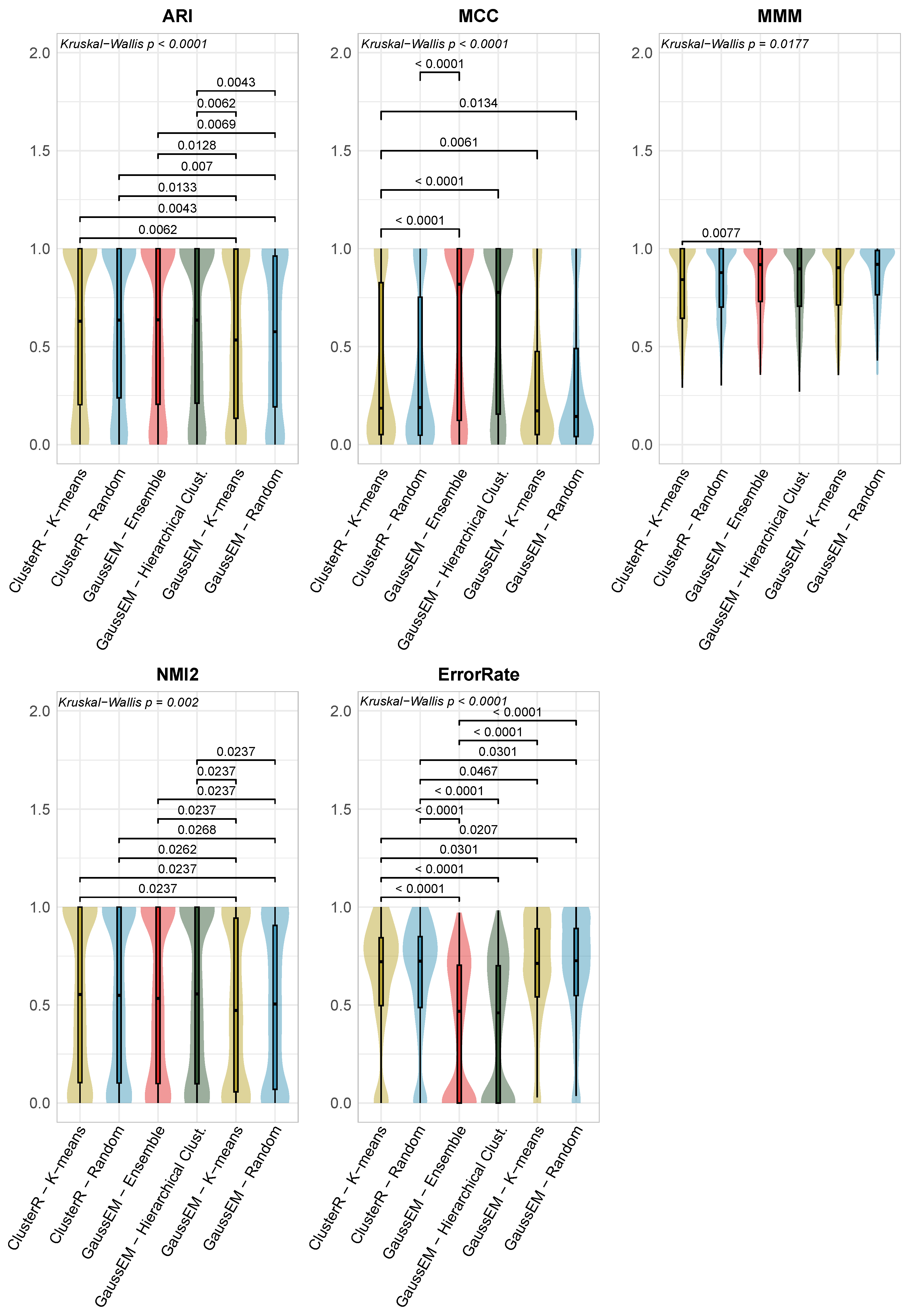
A comparison of the impact of different MDGMM initialization methods on selected quality metrics (ARI, NMI, MCC, MMM, Error Rate) is shown in Figure 1. Each of the five panels presents the distribution of results as violin plots, allowing simultaneous assessment of stability and central values. To verify whether the differences between the approaches were statistically significant, the nonparametric Kruskal-Wallis test [41] was performed (with the significance level set to $\alpha =0.05$). For the statistically significant test results, pairwise comparisons were performed using Conover’s post hoc test [42]. First, quality indices such as ARI and NMI were analyzed. In both cases, Conover’s test showed that the MDGMM with Ensemble and Hierarchical Clustering initialization, as well as ClusterR K-means and random, achieved comparably high effectiveness. In the case of the Error Rate, Ensemble Clustering and Hierarchical Clustering obtained significantly better results than the remaining initialization methods used in MDGMM and in ClusterR. A comparative analysis for MCC, once again, indicated the dominance of Ensemble Clustering and Hierarchical Clustering, which achieved significantly higher results than the remaining methods. At the same time, ClusterR proved to be an intermediate solution, yielding lower results than MDGMM Ensemble and Hierarchical Clustering, but achieving significantly better results than MDGMM, K-means, and random. The MMM metric stood out among the four metrics for its highest stability relative to the initial conditions. While the Conover’s test showed numerous differences in other cases, here, statistical significance was confirmed only for the comparison between Ensemble Clustering and ClusterR K-means. The other configurations were statistically equivalent, as confirmed by the almost identical median levels in the violin plots.

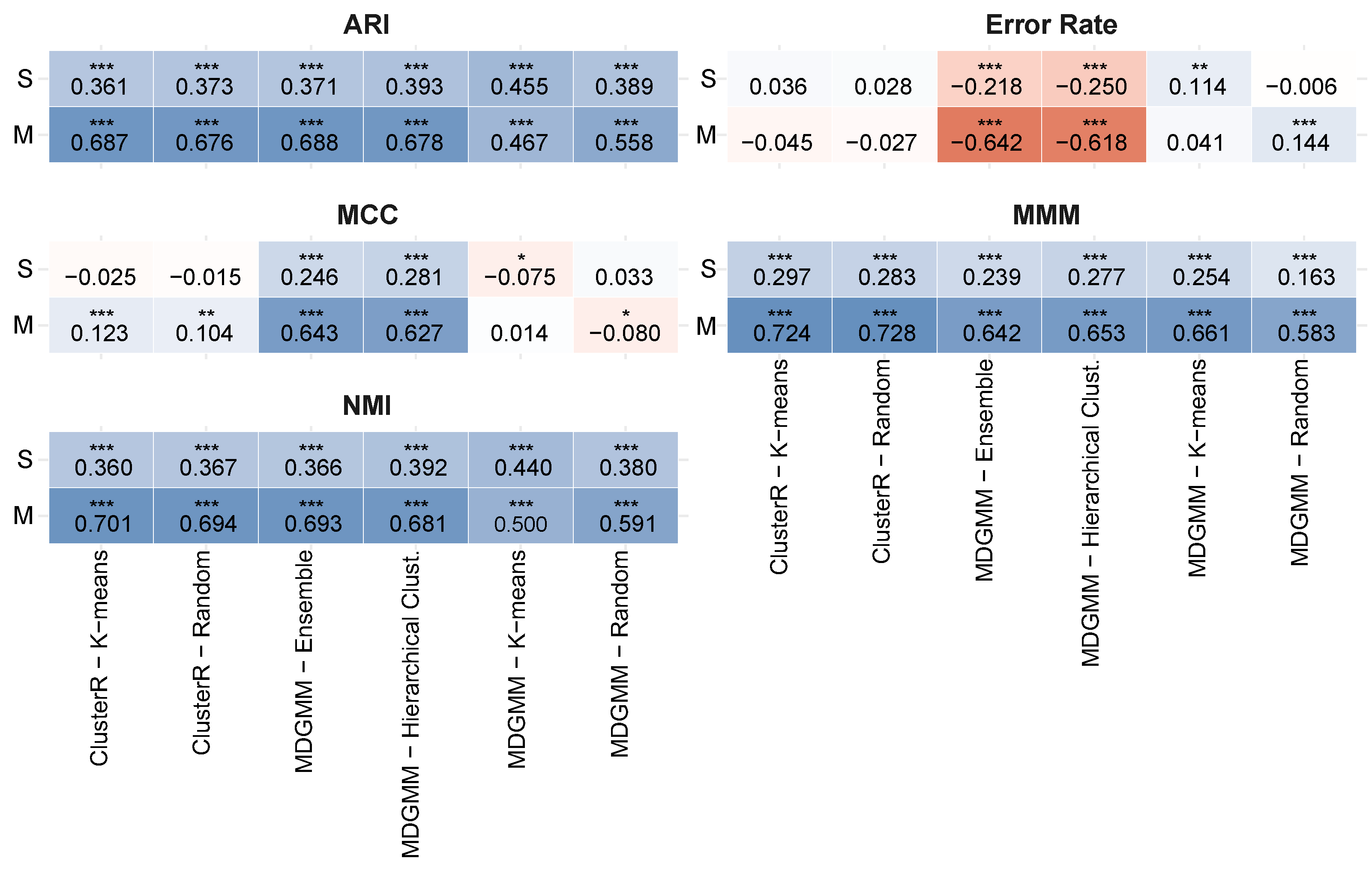
To investigate the influence of dataset parameters, such as separation and the number of dimensions, on quality measure values, a Spearman correlation between the evaluated metrics and the parameters of synthetic datasets with various separations S and dimensions M was calculated for each initialization method. The results are presented in Figure 2.

The graphs show that, in general, increasing S, as with M, improved the quality metrics. The analysis of the MMM, ARI, and NMI metrics revealed a universal dependency pattern common to all initialization methods studied. Both parameters, S and M, showed a constant, positive correlation with the results of this metric at a level of $r_s\in (0.3,0.5)$ for S and $r_s\in (0.45,0.75)$ for M.

A particularly strong correlation was observed for MDGMM Ensemble Clustering in the M, ARI, MCC, and Error Rate metrics, yielding the highest correlation among those metrics compared to other initialization methods. For the MCC metric, the impact of increasing the parameters was limited. Only in the case of Ensemble and Hierarchical Clustering was a statistically significant positive correlation observed: weak for the S parameter and strong for the M parameter. For the other initialization methods tested, the Spearman correlations were, in most cases, not statistically significant. Regarding the Error Rate, statistical analysis showed a highly significant, weak negative correlation with the parameter S and a strong negative correlation with the parameter M for Ensemble and Hierarchical Clustering, indicating that, with increasing S and especially M, the Error Rate decreased markedly in those cases.

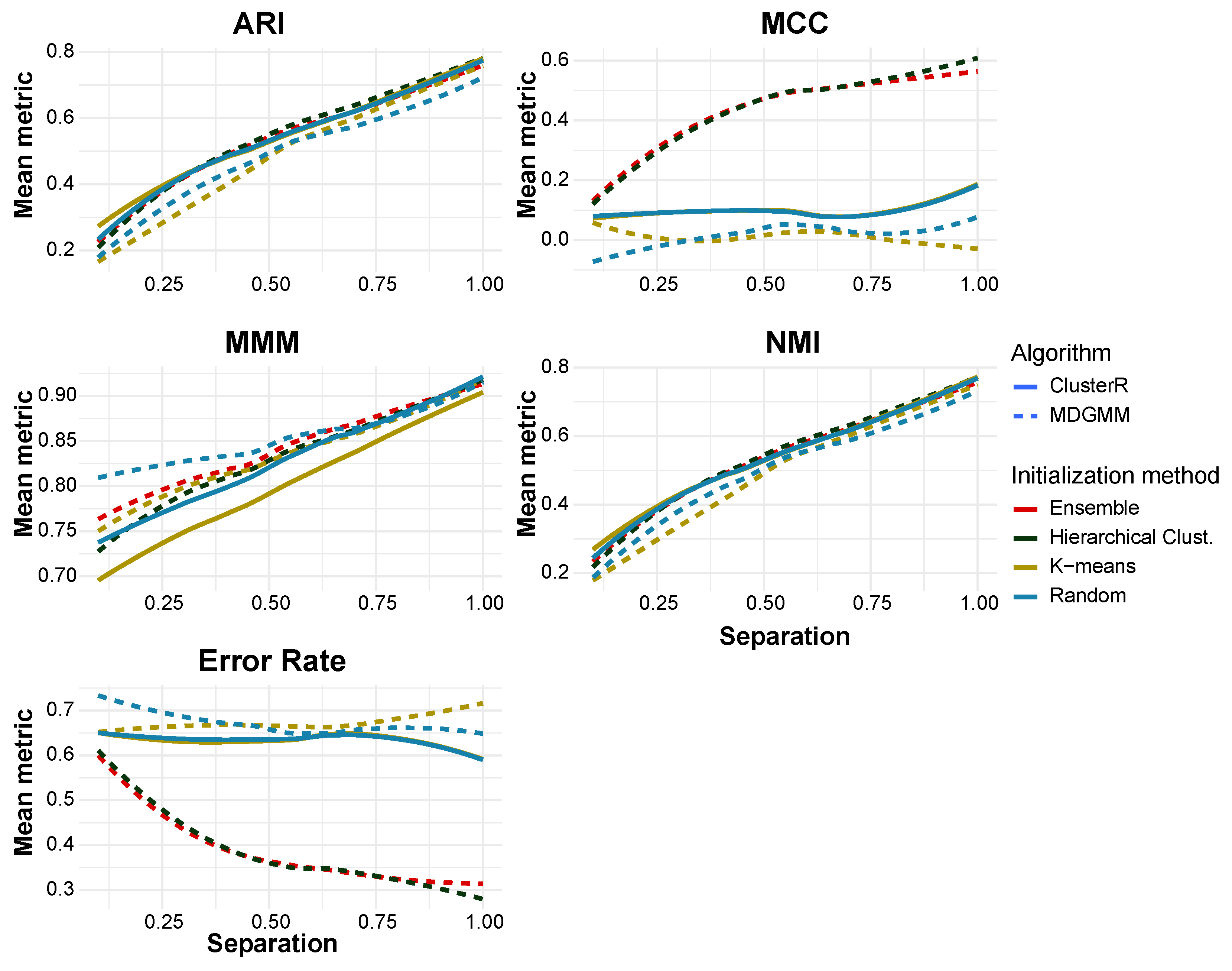
Details on the impact of S on the mean value of each metric across all tested methods are provided in Figure A1. In most cases, increased separation improved clustering quality. For the ARI and NMI metrics, a clear upward trend is evident across all methods, indicating that better-separated clusters are easier to reproduce. A similar effect can be observed for MMM, although the differences between the methods are smaller.

The greatest improvements were observed for MCC and Error Rate. Specifically, as S increased, Ensemble Clustering and Hierarchical Clustering showed a marked improvement, while K-means and random initialization remained weaker. Moreover, the Error Rate decreased significantly for Ensemble and Hierarchical Clustering, but it remained high for the other methods.

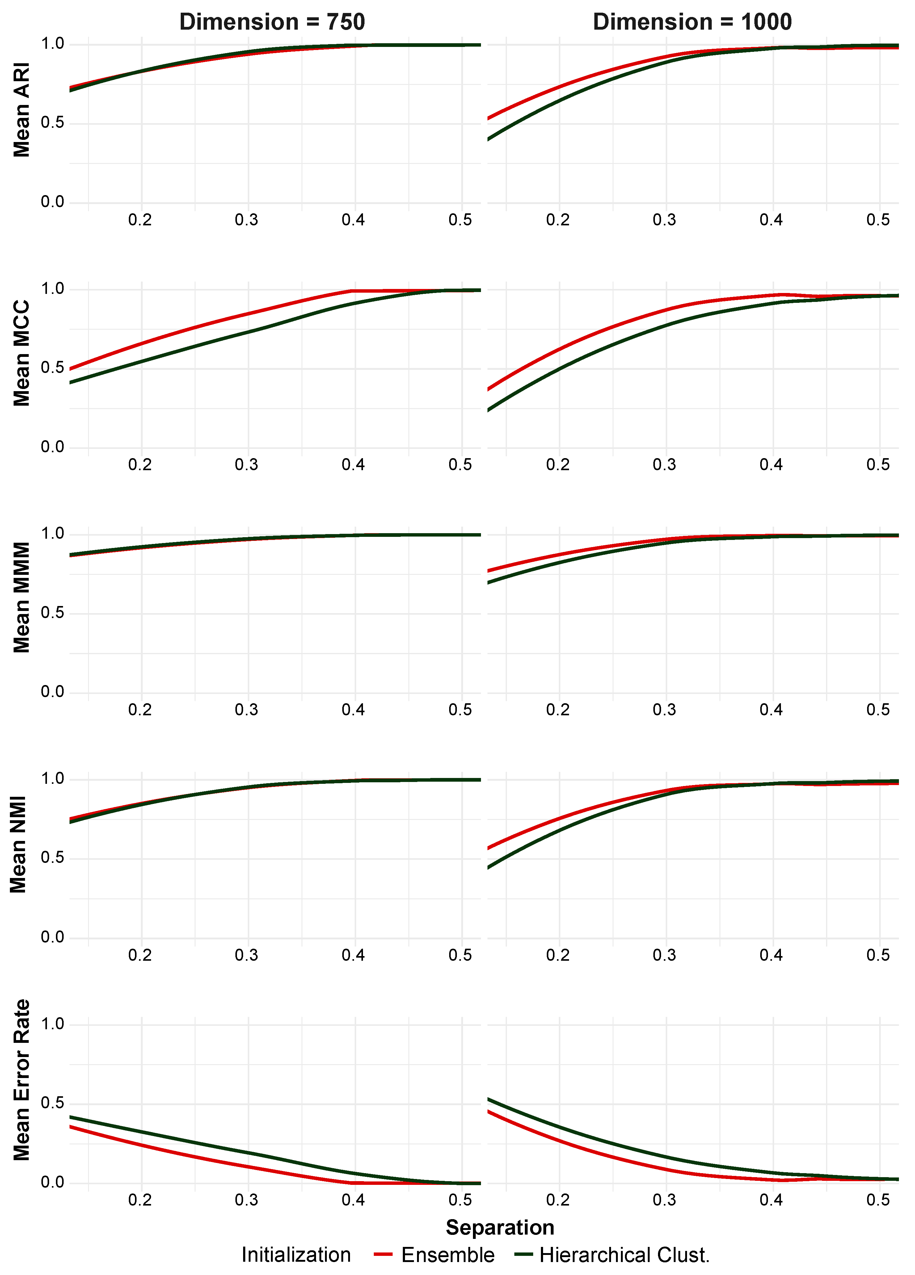
In contrast, Figure A2 shows the results for high dimensionality (M = 750 and M = 1000) and low separation values. Both methods yielded very similar results for all metrics. The advantage of Ensemble Clustering is particularly evident at low S values. For the quality metrics, the values are generally higher, and for the Error Rate, it is lower than in the case of Hierarchical Clustering. The differences are most noticeable for the MCC, NMI, and Error Rate. The effect is stronger for M = 1000, indicating that Ensemble performs better with high cluster overlap and very high dimensionality. As separation increases, the differences disappear, and both methods achieve similar results.

3.2. Real-Word Biological Data

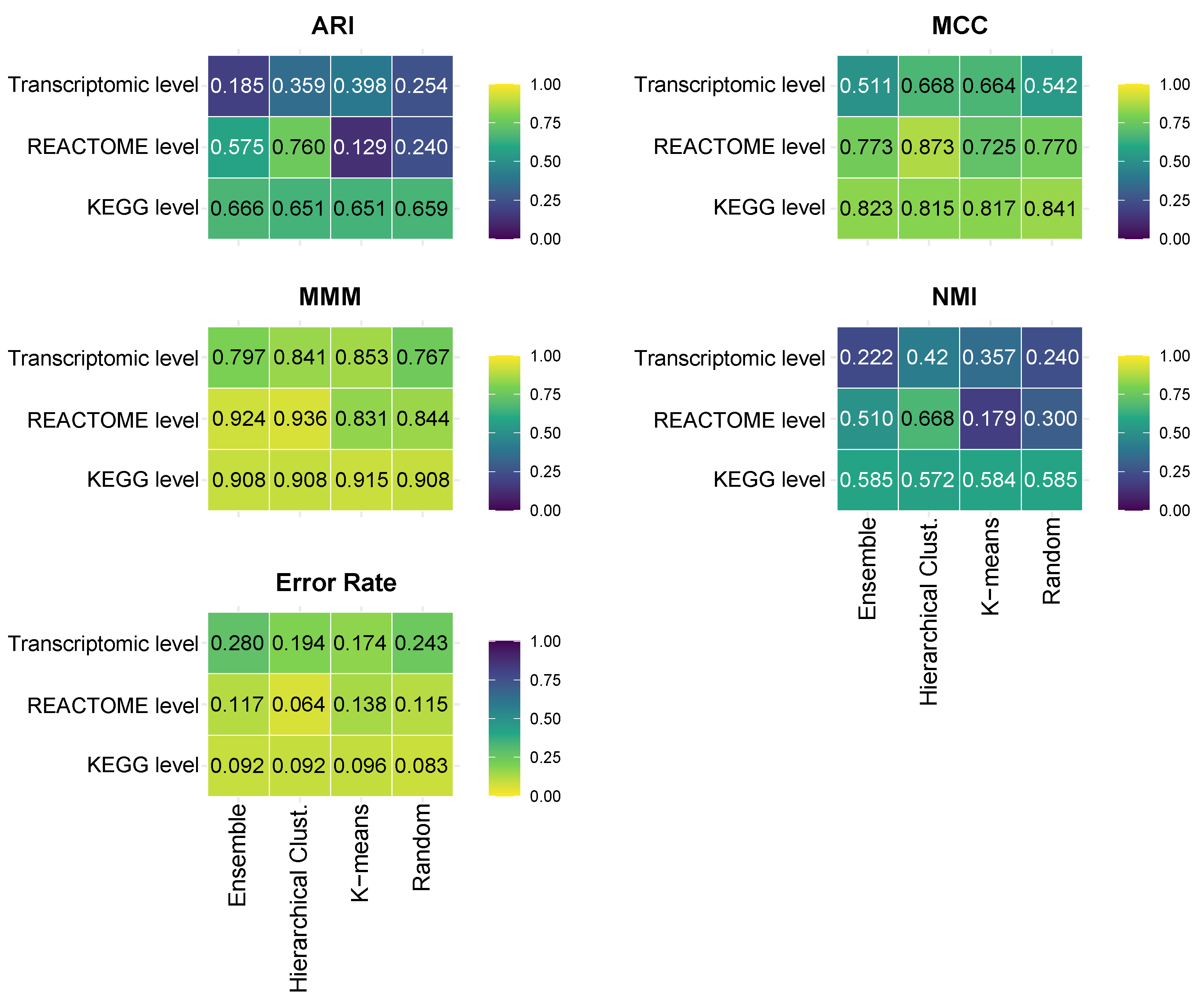
Further, we assessed the impact of the initialization method on the MDGMM results across three real-world biological datasets. To summarize the results obtained on real datasets, a heatmap was used. For each metric studied, a separate matrix was prepared, with rows corresponding to the tested initialization methods and columns to the individual datasets. The results are presented in Figure 3. The values in the map cells represent the medians of the results obtained from samples within the same feature spaces (Transcriptomic-level, KEGG pathways, and REACTOME pathways). The use of the median rather than the arithmetic mean was intended to minimize the impact of outliers on the overall assessment of the methods’ effectiveness.

Heatmap analysis revealed high median values for metrics MCC (indicating good agreement between predicted and true labels) and MMM. Regardless of the dataset or initialization method, the median values of these indicators did not fall below the 0.5 threshold. The MMM metric showed particularly high stability, with values consistently exceeding 0.7.

The analysis of the transcriptomic data revealed a distinct pattern. There was a significant disproportion between the scores obtained using different measures. While metrics based on entropy and pair counting (ARI, NMI) indicated a degradation in clustering quality, the MCC and MMM indicators remained highly stable. The fact that the MCC remained at a satisfactory level (in most cases above 0.6) shows that, despite difficulties in accurately mapping cluster boundaries, the model retains high predictive power and correctly identifies key relationships in the data.

Although the cluster structure is noisy (low NMI) for the most difficult data, the overall Error Rate remained under control (all values were lower than 0.3). This means that the errors are scattered rather than systemic.

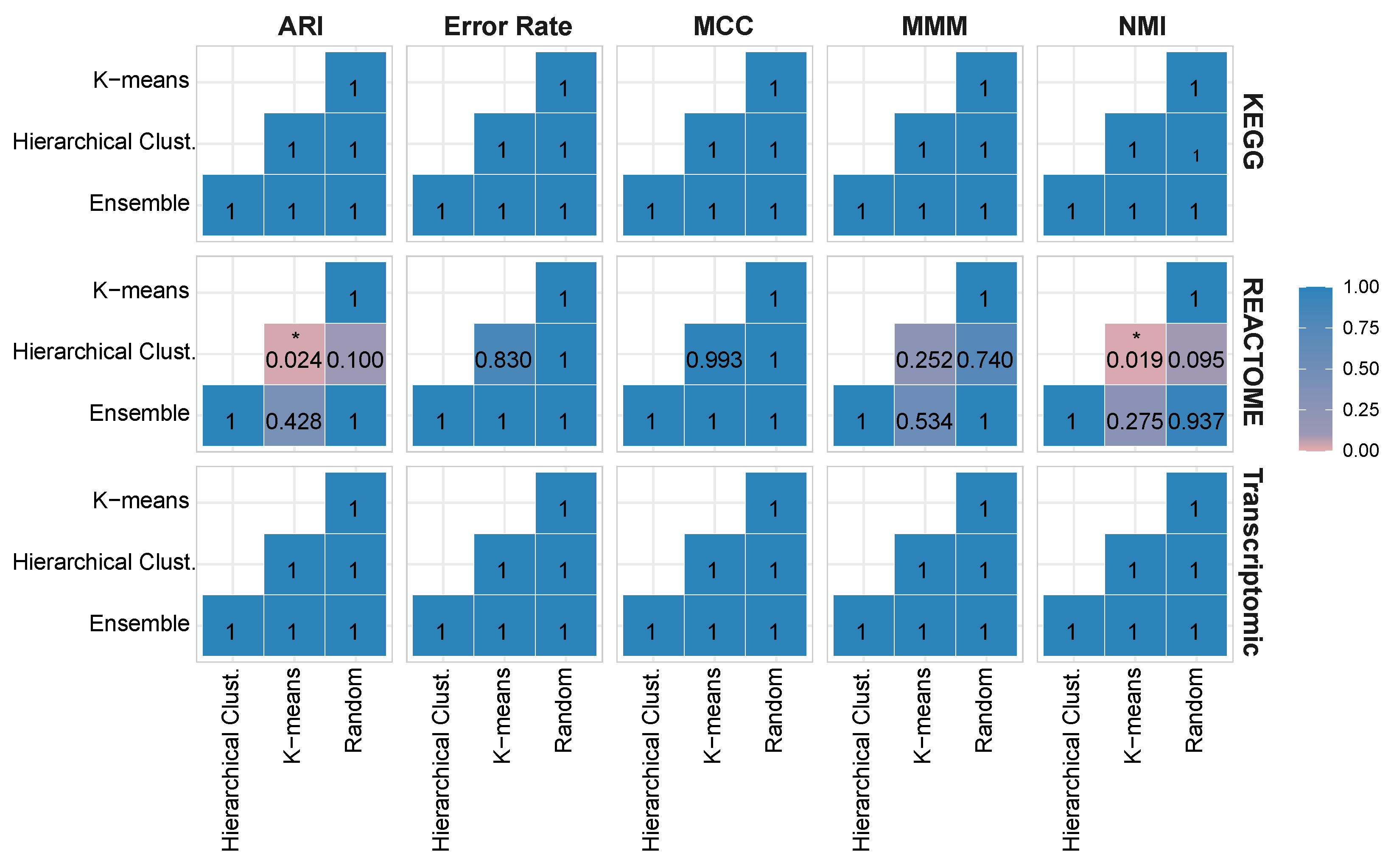
The Kruskal–Wallis test was performed to determine if there were any significant differences in medians among the groups. Then, the Conover’s post hoc test was performed, as in the case of artificially generated data, to identify between which methods there was a significant difference (Figure A3). From the results, we observed significant differences in ARI and NMI metrics only at the REACTOME level between Hierarchical Clustering and K-means. Based on the median values shown in Figure 3, it was concluded that Hierarchical Clustering was more effective than K-means. Moreover, Ensemble did not yield statistically significant improvements compared to other methods.

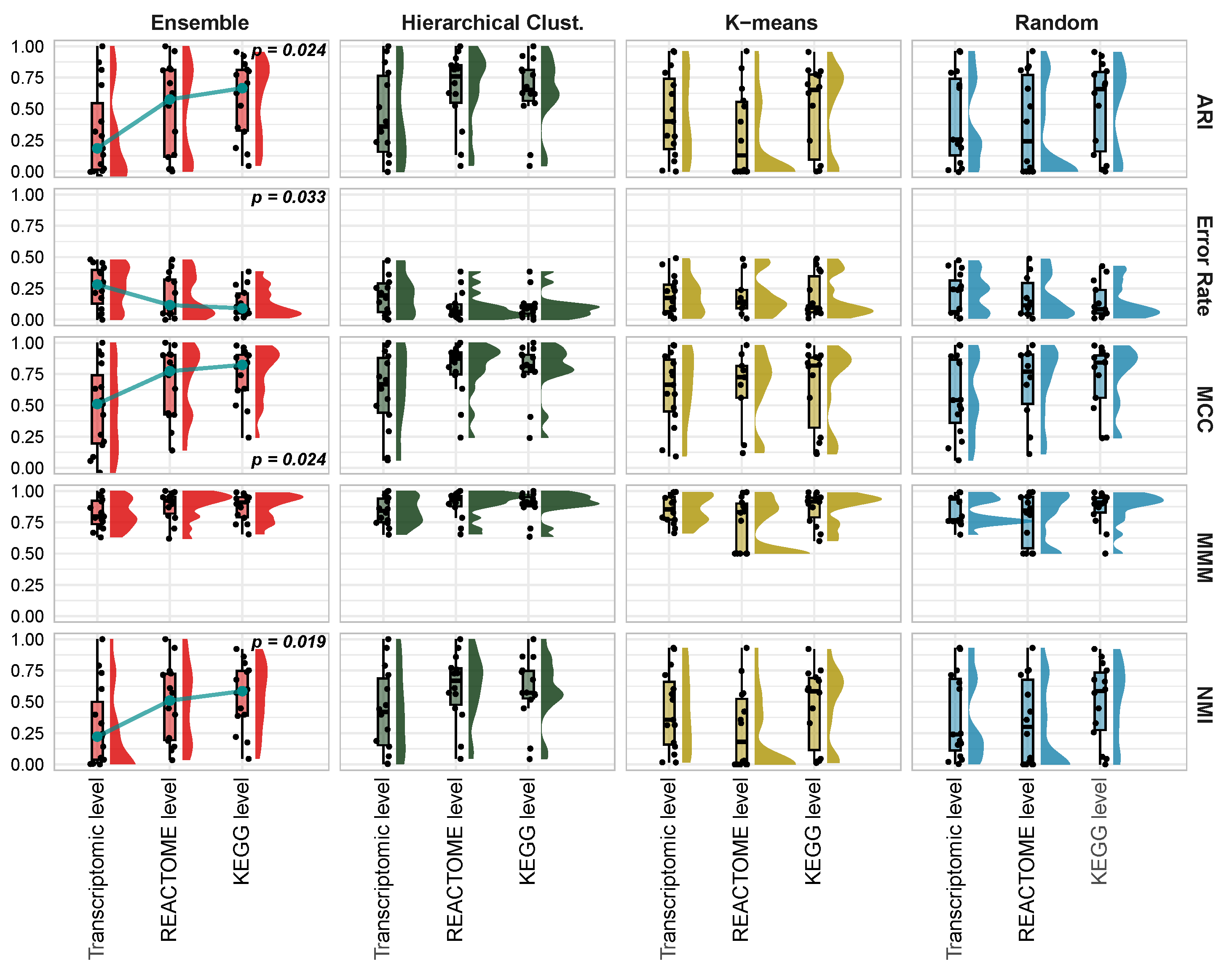
Further, the Jonckheere–Terpstra trend test was performed to evaluate the impact of biological information granularity, ranging from the high-dimensional Transcriptomic level to the more condensed REACTOME and KEGG levels, on clustering performance (Figure A4). This approach accounts for the reduction in feature space while capturing more robust biological signals with diminished stochastic noise. For the MDGMM with Ensemble initialization, the Jonckheere–Terpstra test showed a monotonic increase in the method’s effectiveness ($p<0.05$) across most quality indices. As the number of features decreased across subsequent datasets, improvements in the ARI, MCC, NMI, and Error Rate metrics were observed.

3.3. Computational Time

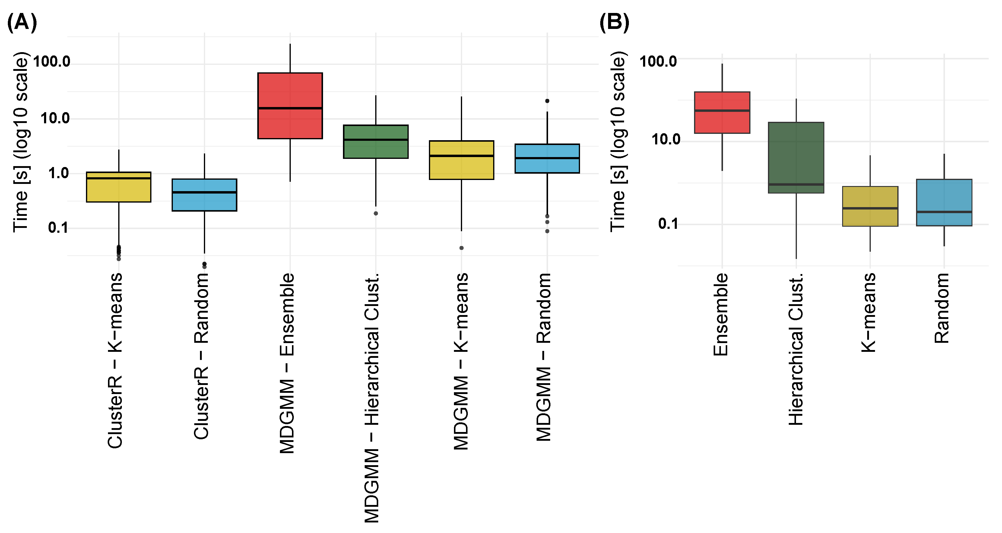
Finally, the empirical computational time of all methods was investigated across both datasets. The results are presented in seconds on a log10 scale on Figure 4. As can be observed in Figure 4A, for synthetic data, the MDGMM–Ensemble initialization is the most computationally demanding among all tested solutions. While the best performance was observed for approaches utilizing K-means and random initializations. Furthermore, for these standard initialization strategies, the MDGMM framework is slower than the corresponding ClusterR implementations. These trends are fully consistent with the performance on real-world biological data (Figure 4B), where the Ensemble approach again exhibits the highest execution time.

4. Discussion

We have performed a comparative study of initialization methods for the MDGMM, random, Hierarchical Clustering, K-means, and Ensemble applied to a range of datasets, both artificially generated and real-life biological datasets. Several clustering quality metrics were used for comparisons: the ARI, MCC, Error Rate, NMI, and MMM.

For artificial datasets, we compared the results of our algorithm with different initialization methods to those obtained with ClusterR GMM using K-means and random initialization. Several clustering quality metrics were used for comparisons: the ARI, MCC, Error Rate, NMI, and MMM. Artificially generated datasets were created with a varying number of observations N, dimensions/number of features M, separation parameter S, and number of clusters/Gaussian components. The number of observations was $N=2000$, number of features ranged from 5 to 1000, and number of mixture components ranged from 2 to 5.

The real datasets included six microarray gene expression datasets and nine RNA sequencing datasets, with observation vectors (patients) ranging from 21 to 226 and features ranging from 10,468 to 17,656. Additionally, real data were categorized into three distinct feature spaces (Transcript-level, KEGG, and REACTOME pathways) to assess whether reducing the feature space for ordered data affects the clustering results.

In this study, the emphasis was on Ensemble Clustering as an initialization for the MDGMM. To investigate whether such MDGMM initialization improves clustering outcomes, a nonparametric Kruskal–Wallis rank-sum test was applied to assess differences in performance across initialization methods, given the non-normal distributions of the results. Conover’s post hoc test was used to perform pairwise comparisons when the Kruskal–Wallis test indicated a statistically significant difference. Spearman’s rank correlation was used to investigate the dependency of the performance metric on the number of features and separation. Furthermore, for real data, the Jonckheere–Terpstra trend test was used to assess the impact of reducing the feature space on ordered data. The significance level was set to $\alpha =0.05$ for all statistical inference procedures. The computational time for each initialization on each dataset was also collected and analyzed.

For the artificially generated datasets, the Kruskal–Wallis rank-sum test, together with Conover’s post hoc test, reveals that initializing MDGMM with Ensemble Clustering and Hierarchical Clustering yielded better clustering performance than the remaining methods across most performance metrics. The MMM remained stable across initialization strategies because they yield a similar number of correctly matched samples after optimal label assignment. This suggests that the overall correspondence between inferred clusters and true labels was largely preserved, even though the detailed clustering structure varied across runs. It can also be concluded that the performance metric’s dependence is strongly correlated with parameters such as the separation S and the dimensions M. For all results, statistically significant positive correlations were observed for the ARI, MMM, and NMI. For the Error Rate and MCC, statistically significant correlations were observed with Ensemble and Hierarchical Clustering.

Analysis of real biological datasets showed that the median values for all metrics were comparable across initialization methods. Further investigation using the Jonckheere–Terpstra trend test revealed that, for the MDGMM with Ensemble initialization, the method showed a monotonic increase in effectiveness across most quality indices, indicating that reducing the dataset’s feature count in subsequent sets improved the ARI, MCC, NMI, and Error rate. Only in the case of the MMM, no improvement was observed. In the biological datasets, stable MMM values suggest that, after optimal label matching, feature-space reduction preserved a similar number of correctly matched samples. This indicates that the main correspondence between clusters and biological reference groups was mostly retained and that the observed grouping was not strongly dependent on a specific reduced feature representation.

The results obtained for high-dimensional data show that the best initialization for MDGMM is provided by two methods: Ensemble Clustering and Hierarchical Clustering. For most of the analyzed quality metrics (ARI, MCC, NMI, and MMM), both algorithms yielded similar results. They achieved better outcomes than classical initializations. Importantly, Ensemble Clustering proved not only comparable to Hierarchical Clustering but also performed better in some scenarios. However, the advantage of the proposed approach is less pronounced for real datasets than for artificially generated data. This may be due to the complexity of biological data, in which clusters are often less clearly separated, might be affected by technical and biological noise. In consequence, clustering performance may be driven more by the intrinsic data structure than by the initialization method, making the proposed approach sometimes comparable to simpler initializations.

The most notable advantage of Ensemble initialization was evident when the separation values were low. This is demonstrated in Figure A2, which compares Hierarchical Clustering and Ensemble Clustering. In that case, the clusters are strongly overlapping, making estimation of the mixture especially challenging. It was exactly when Ensemble methods proved to perform better, achieving higher performance metric values and lower error rates. This suggests that information aggregated from many individual partitions might provide a more stable and accurate starting point for EM iterations, rather than relying on a single hierarchical procedure.

Nonetheless, both methods are computationally intensive. While the empirical execution time of the Ensemble Clustering appeared to rise steadily within the limited scope of the analyzed datasets, especially in the real-world datasets (where the number of observations N was relatively small compared to the feature space M), this empirical observation masks the underlying theoretical complexity. The construction of the $N\times N$ matrix introduces a quadratic time complexity $\mathcal{O}\left(N^2\right)$. Therefore, while ensemble initialization currently offers an attractive compromise between high clustering quality and practical application for moderately-sized datasets, scaling it to massive cohorts, such as the recently introduced single-cell RNA-Seq data (with N usually > 10,000) would require algorithmic optimizations.

References

1. Bouveyron, C.; Celeux, G.; Murphy, T.B.; Raftery, A.E. Model-Based Clustering and Classification for Data Science: With Applications in R; Cambridge University Press: Cambridge, UK, 2019. [Google Scholar]
2. Reynolds, D.A. Gaussian Mixture Models. Encycl. Biom. 2009, 741, 659–663. [Google Scholar]
3. Bouveyron, C.; Brunet, C. Model-Based Clustering of High-Dimensional Data: A review. Comput. Stat. Data Anal. 2013, 71, 52–78. [Google Scholar] [CrossRef]
4. Frühwirth-Schnatter, S.; Celeux, G.; Robert, C.P. Handbook of Mixture Analysis; CRC Press: Boca Raton, FL, USA, 2019. [Google Scholar]
5. Dempster, A.P.; Laird, N.M.; Rubin, D.B. Maximum likelihood from incomplete data via the EM algorithm. J. R. Stat. Soc. Ser. B (Methodol.) 1977, 39, 1–38. [Google Scholar] [CrossRef]
6. Bilmes, J.A. A gentle tutorial of the EM algorithm and its application to parameter estimation for Gaussian mixture and hidden Markov models. Int. Comput. Sci. Inst. 1998, 4, 126. [Google Scholar]
7. McLachlan, G.J.; Peel, D. Finite Mixture Models; John Wiley & Sons: New York, NY, USA, 2000. [Google Scholar]
8. McLachlan, G.J.; Krishnan, T. The EM Algorithm and Extensions; John Wiley & Sons: New York, NY, USA, 2007. [Google Scholar]
9. Zhang, H.; Zhao, L.; Yang, S.; Deng, Y.; Ouyang, Z. Fatigue evaluation of Orthotropic steel deck welds based on WIM data and UD-BP neural network. Structures 2025, 78, 109198. [Google Scholar] [CrossRef]
10. Zyla, J.; Szumala, K.; Polanski, A.; Polanska, J.; Marczyk, M. dpGMM: A new R package for efficient and robust Gaussian mixture modeling of 1D and 2D data. J. Comput. Sci. 2026, 95, 102811. [Google Scholar] [CrossRef]
11. Baudry, J.-P.; Celeux, G. EM for mixtures: Initialization requires special care. Stat. Comput. 2015, 25, 713–726. [Google Scholar] [CrossRef]
12. Karlis, D.; Xekalaki, E. Choosing initial values for the EM algorithm for finite mixtures. Comput. Stat. Data Anal. 2003, 41, 577–590. [Google Scholar] [CrossRef]
13. Biernacki, C. Initializing EM using the properties of its trajectories in Gaussian mixtures. Stat. Comput. 2004, 14, 267–279. [Google Scholar] [CrossRef]
14. Polanski, A.; Marczyk, M.; Pietrowska, M.; Widlak, P.; Polanska, J. Signal partitioning algorithm for highly efficient Gaussian mixture modeling in mass spectrometry. PLoS ONE 2015, 10, e0134256. [Google Scholar] [CrossRef]
15. Polański, A.; Marczyk, M.; Pietrowska, M.; Widłak, P.; Polańska, J. Initializing the EM algorithm for univariate Gaussian, multi-component, heteroscedastic mixture models by dynamic programming partitions. Int. J. Comput. Methods 2018, 15, 1850012. [Google Scholar] [CrossRef]
16. Maitra, R. Initializing partition-optimization algorithms. IEEE/ACM Trans. Comput. Biol. Bioinform. 2009, 6, 144–157. [Google Scholar] [CrossRef] [PubMed]
17. Biernacki, C.; Celeux, G.; Govaert, G. Choosing starting values for the EM algorithm for getting the highest likelihood in multivariate Gaussian mixture models. Comput. Stat. Data Anal. 2003, 41, 561–575. [Google Scholar] [CrossRef]
18. Melnykov, V.; Melnykov, I. Initializing the EM algorithm in Gaussian mixture models with an unknown number of components. Comput. Stat. Data Anal. 2012, 56, 1381–1395. [Google Scholar] [CrossRef]
19. O’Hagan, A.; Murphy, T.; Gormley, I. Computational aspects of fitting mixture models via the expectation-maximization algorithm. Comput. Stat. Data Anal. 2012, 56, 3843–3864. [Google Scholar] [CrossRef]
20. Zhang, H.; Zhao, L.; Chen, F.; Luo, Y.; Xiao, X.; Liu, Y.; Deng, Y. A machine learning and multi-source authentic data-driven framework for accurate fatigue life prediction of welds in existing steel bridge decks. Thin-Walled Struct. 2026, 222, 114559. [Google Scholar] [CrossRef]
21. Panić, B.; Simić, S.; Kovačević, M.; Panić, M. Improved initialization of the EM algorithm for mixture model parameter estimation. Mathematics 2020, 8, 373. [Google Scholar] [CrossRef]
22. Ingrassia, S. A likelihood-based constrained algorithm for multivariate normal mixture models. Stat. Methods Appl. 2004, 13, 151–166. [Google Scholar] [CrossRef]
23. MacQueen, J. Some methods for classification and analysis of multivariate observations. In Proceedings of the Fifth Berkeley Symposium on Mathematical Statistics and Probability; University of California Press: Oakland, CA, USA, 1967; pp. 281–297. [Google Scholar]
24. Arthur, D.; Vassilvitskii, S. K-means++: The advantages of careful seeding. In Proceedings of the Eighteenth Annual ACM-SIAM Symposium on Discrete Algorithms, New Orleans, LA, USA, 7–9 January 2007; Society for Industrial and Applied Mathematics: Philadelphia, PA, USA, 2007; pp. 1027–1035. [Google Scholar]
25. Murtagh, F.; Contreras, P. Algorithms for hierarchical clustering: An overview. Wiley Interdiscip. Rev. Data Min. Knowl. Discov. 2012, 2, 86–97. [Google Scholar] [CrossRef]
26. Ward, J.H., Jr. Hierarchical grouping to optimize an objective function. J. Am. Stat. Assoc. 1963, 58, 236–244. [Google Scholar] [CrossRef]
27. Fred, A.L.N. Finding consistent clusters in data partitions. In Multiple Classifier Systems; Kittler, J., Roli, F., Eds.; Springer: Berlin/Heidelberg, Germany, 2001; pp. 309–318. [Google Scholar]
28. Fred, A.L.N.; Jain, A.K. Robust data clustering: A combiner approach. In Proceedings of the IEEE Computer Society Conference on Computer Vision and Pattern Recognition (CVPR); IEEE: Madison, WI, USA, 2003; pp. 128–136. [Google Scholar]
29. Mouselimis, L. R Package, version 1.3.6; ClusterR: Gaussian Mixture Models, K-Means, Mini-Batch-Kmeans, K-Medoids and Affinity Propagation Clustering; CRAN: Vienna, Austria, 2025.
30. Sanderson, C.; Curtin, R. Armadillo: A template-based C++ library for linear algebra. J. Open Source Softw. 2016, 1, 26. [Google Scholar] [CrossRef]
31. Widłak, W. High-Throughput Technologies in Molecular Biology. In Molecular Biology. Lecture Notes in Computer Science; Widłak, W., Ed.; Springer: Berlin/Heidelberg, Germany, 2013; Volume 8248. [Google Scholar] [CrossRef]
32. Geistlinger, L.; Csaba, G.; Santarelli, M.; Ramos, M.; Schiffer, L.; Turaga, N.; Waldron, L. Toward a gold standard for benchmarking gene set enrichment analysis. Brief. Bioinform. 2021, 22, 545–556. [Google Scholar] [CrossRef] [PubMed]
33. Barbie, D.A.; Tamayo, P.; Boehm, J.S.; Kim, S.Y.; Moody, S.E.; Dunn, I.F.; Hahn, W.C. Systematic RNA interference reveals that oncogenic KRAS-driven cancers require TBK1. Nature 2009, 462, 108–112. [Google Scholar] [CrossRef]
34. Kanehisa, M.; Goto, S. KEGG: Kyoto encyclopedia of genes and genomes. Nucleic Acids Res. 2000, 28, 27–30. [Google Scholar] [CrossRef]
35. Jassal, B.; Matthews, L.; Viteri, G.; Gong, C.; Lorente, P.; Fabregat, A.; D’Eustachio, P. The reactome pathway knowledgebase. Nucleic Acids Res. 2020, 48, D498–D503. [Google Scholar] [CrossRef]
36. Santos, J.M.; Embrechts, M. On the use of the adjusted Rand index as a metric for evaluating supervised classification. In Proceedings of the International Conference on Artificial Neural Networks; Springer: Berlin/Heidelberg, Germany, 2009; pp. 175–184. [Google Scholar]
37. Hubert, L.; Arabie, P. Comparing partitions. J. Classif. 1985, 2, 193–218. [Google Scholar] [CrossRef]
38. Chicco, D.; Jurman, G. The advantages of the Matthews correlation coefficient (MCC) over F1 score and accuracy in binary classification evaluation. BMC Genom. 2020, 21, 6. [Google Scholar] [CrossRef] [PubMed]
39. Hastie, T.; Tibshirani, R.; Friedman, J. The Elements of Statistical Learning: Data Mining, Inference, and Prediction, 2nd ed.; Springer: New York, NY, USA, 2009. [Google Scholar]
40. Cai, D.; He, X.; Han, J. Document clustering using locality preserving indexing. IEEE Trans. Knowl. Data Eng. 2005, 17, 1624–1637. [Google Scholar] [CrossRef]
41. Kruskal, W.H.; Wallis, W.A. Use of ranks in one-criterion variance analysis. J. Am. Stat. Assoc. 1952, 47, 583–621. [Google Scholar] [CrossRef]
42. Conover, W.J. Practical Nonparametric Statistics, 3rd ed.; John Wiley & Sons: New York, NY, USA, 1999. [Google Scholar]
43. Jonckheere, A.R. A distribution-free k-sample test against ordered alternatives. Biometrika 1954, 41, 133–145. [Google Scholar] [CrossRef]
Figure 1. Comparison of initialization methods across metrics. Within each metric, initialization methods were compared using pairwise Conover’s post hoc tests, and statistically significant differences are indicated.
Applsci 16 05427 g001
Figure 2. Spearman rank correlation coefficient between initialization methods and two synthetic data parameters (number of dimensions M and separation S). Statistical significance is marked as follows: * p < 0.05, ** p < 0.01, *** p < 0.001.
Applsci 16 05427 g002
Figure 3. Comparison of median value of evaluation metrics for different initializations and HT data levels. The color scale ranges from yellow to purple, with yellow indicating good performance and purple indicating poor performance.
Applsci 16 05427 g003
Figure 4. Computational time (log10 scale) for tested initializations and dataset collections. Panel (A) shows result for artificially generated data, while panel (B) shows real-world biological data results. The dots represents the outliers.
Applsci 16 05427 g004