Article

Integrated Modeling and Data-Driven Analysis of Bread Machine Electromechanical System with Hydration-Dependent Viscoelastic Load

Faculty of Technics and Technologies, Trakia University, 38 Graf Ignatiev Street, 8602 Yambol, Bulgaria
*
Author to whom correspondence should be addressed.
Appl. Sci. 2026, 16(11), 5392; https://doi.org/10.3390/app16115392
Submission received: 14 April 2026 / Revised: 18 May 2026 / Accepted: 25 May 2026 / Published: 28 May 2026

Abstract

Electromechanical systems operating under viscoelastic loads require precise modeling due to the highly nonlinear behavior of the load. An automatic bread machine is a practical example where dough represents a dynamic viscoelastic load sensitive to hydration. As found in this paper, increasing the water content leads to a decrease in the torque and the required mechanical power. An integrated approach combining MATLAB/Simulink and Simscape modeling, experimental measurements, and a PCA-based regression model is presented. The tests were conducted with three types of flour (type 500, type 1850, and rye–wheat) at hydrations of 52%, 58%, and 63% with over 6000 measurements recorded for each combination. The regression models achieve moderate predictability (R2 = 0.64–0.96) model performance that varies across flour types. Increasing the dough hydration from 52% to 63% reduces the torque by approximately 22–46% across the tested flour types, while the angular velocity rises slightly (from about 147.9 to 151.9 rad/s). A descriptive decrease in energy consumption of up to around 6% was observed within the sampled batches with the system efficiency remaining within a narrow range around η ≈ 0.67. Within the studied levels (52–63%), the minimum load was observed at 58%. The proposed integrated model reliably describes the interaction between the electric motor, the mechanical gear, and the viscoelastic load, and it offers a basis for energy optimization and the implementation of low-cost sensor systems for intelligent control in the bread-making process.

1. Introduction

Electromechanical devices convert energy between electrical and mechanical forms. The behavior of the mechanical load plays a major role in how efficient, stable, and reliable these systems are, especially when the load shows viscoelastic properties [1]. This type of behavior appears in many industrial and biomedical settings, such as material-handling mechanisms and electric-drive control systems [2]. Because the interactions between components change over time and are often complex, traditional analytical models are not always enough. As a result, data-driven approaches are becoming increasingly important for achieving better accuracy [3].
Recent research pays particular attention to electromechanical systems that operate under variable and dynamic loads [4]. An automated bread-making machine is a practical example for studying such conditions. Its electric drive goes through repeated phases of mixing, resting, fermentation, and heating. Each stage brings rapid torque changes, high starting currents, mechanical impacts from the dough, and temperature fluctuations [5]. Since these machines are compact yet energy-intensive, they provide a useful platform for examining how dynamic loads affect system performance, product quality, and overall energy use [6].
Recent publications in the field of small-scale food processing technologies highlight a growing interest in automated bread-making devices, which is driven by advances in intelligent control, energy-efficient electromechanical design, and integrated sensor systems. Current research trends focus on improving process monitoring, optimizing mixing dynamics, and enhancing system reliability through embedded sensing and data-driven analysis. These developments position household bread machines as suitable platforms for studying electromechanical systems operating under variable viscoelastic loads [7,8,9,10].
Even with their popularity, automatic bread machines pose notable challenges from both mechanical and control perspectives. Dough has complex viscoelastic behavior, which means its response changes over time and does not follow simple linear rules [11,12,13]. This directly affects how efficiently the machine can knead the dough and how good the final bread will be. The dough’s rheological properties, strongly shaped by hydration, play a key role in forming the gluten network, developing texture, and guiding fermentation [14,15,16]. Because these properties vary widely with ingredients and conditions, accurately modeling and controlling the process remains difficult.
A large body of research has examined different aspects of dough preparation and bread-machine operation, which are typically grouped into three areas: dough-mixing mechanisms, fermentation monitoring, and data-driven quality prediction. Studies on mixing systems include the mechanical designs proposed by Okafor [17], Orelaja et al. [18], and Abdul Fatah et al. [19], which improve efficiency, dough uniformity, or processing time. However, these works treat the mixer primarily as a mechanical subsystem and do not analyze the coupled interaction between the motor, transmission, and the viscoelastic dough.
Research on fermentation control, such as the electromechanical monitoring approach developed by Hsu [20], focuses on identifying optimal baking conditions but does not characterize the mechanical load during mixing. Data-driven approaches to bread-quality prediction, including the neural-network-based method of Lee et al. [21], rely on sensory or visual features and provide limited insight into the internal electromechanical behavior of the machine.
Simulation tools such as MATLAB, Simulink, and Simscape have been used for the system-level modeling of electromechanical devices [22,23,24], while earlier studies have demonstrated how physical systems can be translated into simulation models and optimized under varying conditions [25,26]. Additional tools such as ElectroM extend these capabilities to nonlinear systems [27]. Despite their strengths, these approaches often rely on simplified load representations and require experimental validation when applied to nonlinear viscoelastic materials such as dough.
The main contributions of this paper are as follows:
(1)
An integrated electromechanical–viscoelastic model combining Simscape physics and PCA-based analysis;
(2)
Experimentally validated relationships between dough hydration, torque demand, angular velocity, and energy consumption;
(3)
A low-cost sensor-based measurement system enabling the real-time monitoring of torque, speed, and power in bread-making machines.
No prior study integrates electromechanical modeling, hydration-dependent viscoelastic load characterization, and PCA-based analysis into a unified framework validated with high-resolution experimental data. By combining system-level modeling, experimental measurements, and data-driven analysis, the proposed approach offers a strong foundation for improving energy efficiency, process stability, and product quality in electromechanical systems operating with complex viscoelastic loads.
The paper is organized as follows. Section 2 presents the materials, experimental setup, and the integrated modeling approach, including the physical and data-driven components. Section 3 reports the experimental results and the validation of the electromechanical-viscoelastic model. Section 4 examines how dough hydration and flour type influence the electromechanical behavior of the system in terms of torque demand, angular velocity stability, and energy consumption, while also summarizing the main findings and methodological limitations, and identifying directions for future work.

2. Material and Methods

In the integrated model of the electromechanical control system of an automatic bread machine, two levels of abstraction are used, which combine a physical and a computational model of the system. The first level is a system physical model of the electric motor, the mechanical gear, and the viscoelastic load, which is described by equations for current, torque, angular velocity, inertia, and friction. This allows for an analysis of the dynamic modes and the interaction between the electric drive and the dough. The second level is a functional model based on PCA analysis, which summarizes the experimental data and predicts the load on the electromechanical system, depending on the hydration and type of flour. The combination of the two levels provides a sufficiently effective simulation of real operating modes and the possibility of improving the performance of the electromechanical system based on actually measured data.

2.1. Place and Conditions of Measurement

The measurements were made in the laboratories of “Production Automation and Robotics” and “Food Technologies” at the Faculty of “Technics and Technology”, Yambol, Bulgaria. In all cases, the measurements are carried out at the same altitude. The atmospheric pressure and gas composition of the air are assumed to be constant and are not taken into account. The measurements were made at a temperature of 20 ± 3 °C and a relative humidity of 40 ± 3%RH.
To ensure reproducibility and to address the dynamic nature of the electromechanical load, all measurements were performed under controlled and repeatable conditions.
All electrical and mechanical signals (voltage, current, motor speed, temperature) were sampled at 100 Hz, which provides sufficient temporal resolution to capture the rapid torque fluctuations during kneading. The sampling frequency was selected based on preliminary tests showing that higher rates did not change the measured signal characteristics in a meaningful way.
Each measurement sequence covered the entire kneading phase, lasting 12 min for all flour types and hydration levels. Only the steady-state portion of the kneading cycle (between 1 min and 3 min) was used for analysis to avoid transient effects at startup and shutdown. The interval between 1 and 3 min was identified as the quasi-steady operating region based on the stabilization of motor current, torque, and angular velocity, which was confirmed through preliminary exploratory analysis of the time-series data.
For each flour type and hydration level, three independent dough batches were prepared and measured. This ensured that the dataset did not consist of autocorrelated samples from a single batch and allowed for an assessment of batch-to-batch variability. Each batch produced approximately 6000 data points, resulting in more than 18,000 samples per condition.
Raw signals were preprocessed using a second-order low-pass Butterworth filter with a cutoff frequency of 10 Hz to suppress high-frequency electrical noise and mechanical vibration artifacts. Filtering was applied identically to all signals to maintain consistency across conditions.
All sensors were calibrated prior to data collection. The ACS712 current sensor was calibrated using a laboratory power supply and a precision ammeter (±1% accuracy). The voltage measurement circuit was calibrated against a true-RMS multimeter. The F249 speed sensor was calibrated using a reference motor with known rotational speed. The thermocouple amplifier (MAX6675) was calibrated using a certified temperature probe in the range 20–60 °C. Calibration curves were applied to all raw measurements before further processing.

2.2. Test Measurements and Raw Materials Used

Test measurements of the characteristics of an electromechanical system of an automatic bread machine were made using a viscoelastic load—bread dough.
The following raw materials were used: flour type 500 (white) (GoodMills Bulgaria EOOD, Sofia, Bulgaria); flour type 1150 (standard) (GoodMills Bulgaria Ltd., Sofia, Bulgaria); flour type 1850 (whole grain) (GoodMills Bulgaria Ltd., Sofia, Bulgaria); rye flour type 1750 (SP. “TIT-Tenyo Tenev,” Kameno, Bulgaria); drinking water, according to Regulation No. 9/2001 on the quality of water intended for drinking and domestic purposes of the Ministry of Health, Ministry of Regional Development and Public Works, and Ministry of Environment and Waters (published in the State Gazette, issue 30, 2001).
The dough was prepared according to approved Bulgarian bread standards (https://bfsa.egov.bg, accessed on 31 May 2025): US02/2011 White Bread; US07/2019 Whole Wheat Bread; US09/2019 Rye–Wheat Bread.
According to the specified standards, water was added in quantities of 52–63% to the flour (or flour mixture). The rye–wheat dough (60/40%) was made only with a flour mixture and water without liquid rye sourdough. The dough was prepared with 300 g of flour or flour mixture with quantities of water specified in the standards above.

2.3. Selection of Measuring and Control Devices for a System for Determining the Dynamic Characteristics of an Automatic Bread Machine

Table A2 of Appendix A presents the hardware used to build a device for determining the characteristics of an electromechanical system of an automatic bread machine.
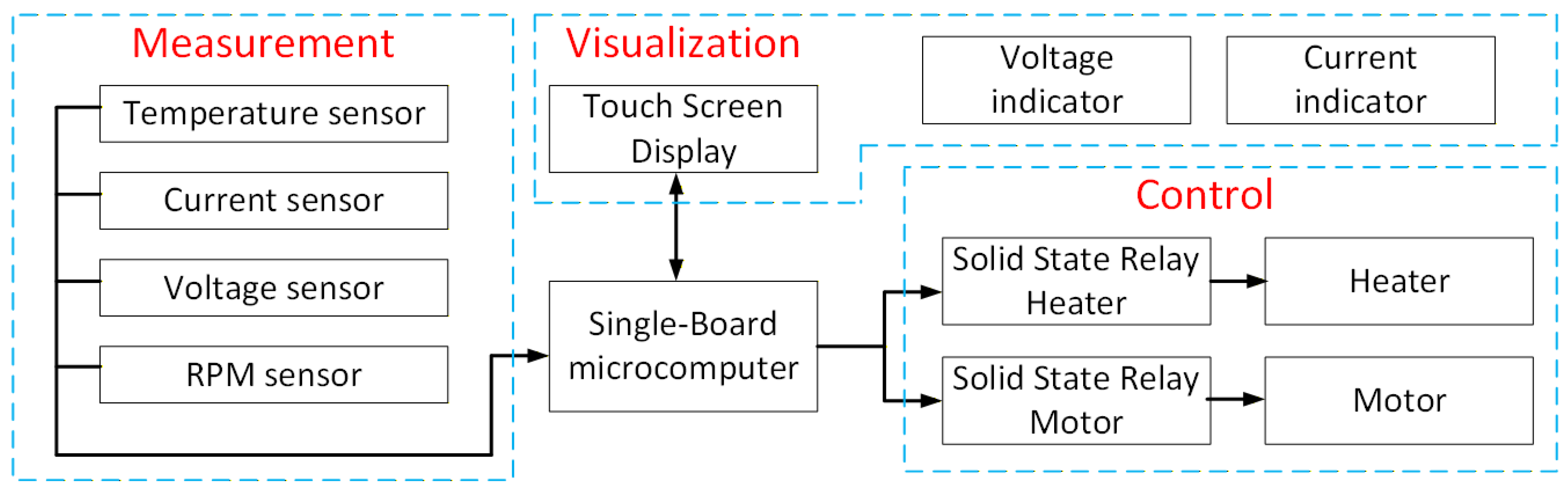
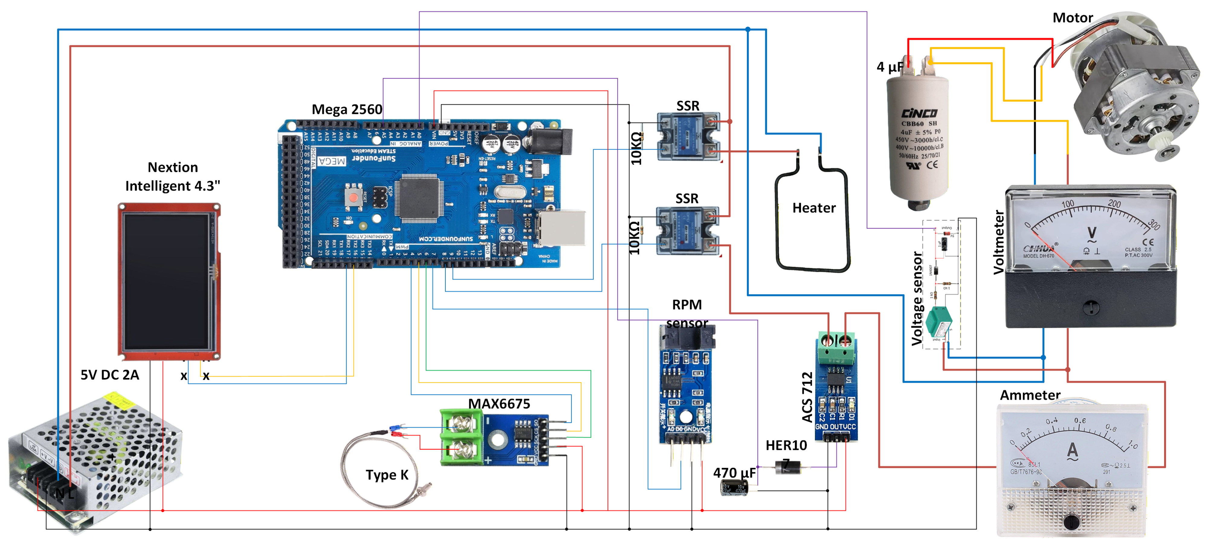
Figure 1 shows a block-diagram of the proposed electric drive measurement and control system. On the left side are the four main sensors—for temperature, current, voltage, and speed, which feed data to the Mega 2560 single-board microcomputer. It performs the functions of a central controller, processing incoming signals, calculating the current parameters of the electromechanical system, and controlling the actuators. The upper part shows the visualization module, implemented using the Nextion touch display, which provides two-way communication with the controller and allows for the monitoring of the measured values and interaction with the operator. On the right side are the control channels to the semiconductor relays for the electric motor and heater, which ensure the execution of the commands for controlling the electromechanical system.
The characteristics of the electric motor of the automatic bread machine are presented in Table 1. The nominal voltage and power are according to the technical specification of the electric motor. The nominal current of the electric motor was measured with a digital multimeter UNI-T UT20B (Uni-Trend Group Ltd., Chengdu, China). The resistance and inductance of the windings were determined with a measuring instrument UNI-T UT603 (Uni-Trend Group Ltd., Chengdu, China).
The synchronous speed Ns, rpm is determined by
N s = 120 f p , r p m
where f represents the frequency of the supply voltage, which is measured in Hz; and p represents the number of poles of the electric motor.
The slip of the electric motor S is determined by
S = N s N n N s , a . u .
where Ns represents the synchronous speed of the electric motor, which is measured in rpm; and Nn represents the nominal speed of the electric motor, which is also measured in rpm.
The nominal torque Tn is determined by
T n = P n ω n , N m
where Pn represents the nominal power of the electric motor, which is measured in W; and ωn represents the nominal angular velocity of the electric motor, which is measured in rad/s.
The initial data for the mechanical transmission of the automatic bread machine are presented in Table 2. The dimensions were determined with a digital caliper SEB-DC-023 (Shanghai Shangerbo import & export Co., Ltd., Shanghai, China) with an accuracy of 0.05 mm and a maximum measured length of 150 mm. The efficiency of the belt transmission was determined according to catalog data.

2.4. Determining the Characteristics of an Electromechanical System

The electromechanical system converts electrical energy into mechanical energy. The electric motor, belt drive, and dough have a dynamic interaction. The computational equations for this type of electromechanical system are adapted from those presented in the available literature [28,29,30,31]. The principle of conversion from integral to a form usable in a computational program, which is based on discretization, is used. In this, continuous physical quantities and integrals are replaced by finite values measured at separate moments of time, and the integrals are approximated by sums. This allows the relatively complex dependencies described by integrals to be calculated numerically by computer program algorithms that use step intervals and repeated calculations. The equations used are presented in both integral and discrete forms. The integral control equation is expressed as
W m = t 0 t 1 P m t d t , J
where Wm is the mechanical work, which is measured in J; and Pm is the mechanical power, which is measured in W. The induced electromechanical force (EMF) (induced EMF) is defined by
E t = U t R I t L d I d t , V
where E is the EMF, which is measured in V; U is the measured voltage of the motor, which is measured in V; I is the current of the motor, which is measured in A; R is the resistance of the motor windings, which is measured in Ω; and L is the inductance of the motor windings, which is measured in H. Basically, the EMF is obtained as the difference between the voltage applied to the motor and the losses in the resistance and inductance of the windings. This is directly related to Faraday’s law of electromagnetic induction, which states that changes in magnetic flux induce a voltage.
The mechanical work P and mechanical energy W generated by the motor are defined by
W m = t 0 t 1 T t ω t d t , J
P m = T ω , W
where Pm is the mechanical power, which is measured in W; Wm is the mechanical energy, which is measured in J; T is the torque, which is measured in Nm; ω is the angular velocity in rad/s, and Pm is the mechanical work in W. The mechanical work is used to calculate the total mechanical energy transmitted by the electric motor for a given interval.
The mechanical power is used to determine the instantaneous power produced by the torque and the angular velocity. The mechanical power is calculated for both the electric motor and the agitator, taking into account the conversion factor:
P m _ m i x = T m i x ω m i x , W
where Tmix is the torque of the drive mechanism, which is measured in Nm; ωmix is the angular velocity of the stirring mechanism, which is measured in rad/s; and Pm is the mechanical work, which is measured in W.
The electric power P and the electric energy We of the electric motor are determined by
W e t = t 0 t 1 U t I t d t , J
P = U . I . c o s ( φ ) , W
where U is voltage, which is measured in V; I is electric current, which is measured in A; cos(φ) is the power factor, which is measured in a.u.; Pe is electric power; and We is electric energy, which is measured in J. We represent the total electric energy delivered to the motor and the instantaneous electric power.
The power factor of an electric motor is determined by
c o s ( φ ) = P w m S
S = U I , V A
c o s ( φ ) = P w m U I
where cos(φ) is the power factor, which is measured in a.u.; U is the voltage, which is measured in V; I is the electric current, which is measured in A; Pwm is the active power, which is directly measured with a wattmeter; and S is the apparent power, which is measured in VA.
The efficiency of the electromechanical system is calculated by:
η = P m _ m i x P
where η is the efficiency of the electromechanical system, which is measured in a.u.; Pm_mix is the mechanical power, which is measured in W; and P is the electrical power of the electric motor, which is measured in W.
The torque T of the electric motor, which is measured in Nm, is determined by
T = P 2 π N 60 , N m
where P is the electric power of the electric motor, which is measured in W; and N is the speed of the electric motor, which is measured in rpm.
The torque Tmix at the mixing element is determined by
T m i x = T D m i x D η , N m
W m i x = t 0 t 1 T m i x t ω m i x t d t , J
where T is the torque of the electric motor, which is measured in Nm; D is the diameter of the drive wheel of the belt drive (at the motor), which is measured in m; Dmix is the diameter of the driven wheel (at the stirring element), which is measured in m; η is the efficiency of the belt drive (assumed to be 0.95), which is measured in a.u.; and Wmix is the mechanical energy, which is measured in J.
The angular speed (velocity) ω is calculated by
ω = 2 π N 60 , r a d / s
where N is the speed of the electric motor, which is measured in rpm. For the mixing mechanism, it is calculated in the same way as Nmix, and the rpm is recalculated with the gear ratio of the belt drive.
The tension force in the belt drive is determined by
W b = t 0 t 1 F 1 t F 2 t ω ( t ) d t , J
F 1 F 2 = P m ω , N
where F1 is the tensile force of the driving disk, which is measured in N; F2 is the tensile force of the driven disk, which is measured in N; Pm is the mechanical power, which is measured in W; ω is the angular velocity, which is measured in rad/s; and Wb is the energy of the belt drive, which is measured in J. It determines the difference in the tensile forces of the driving and driven disks.
Figure 2 shows a diagram of the forces acting in the belt drive. A belt drive with two discs and a belt is visualized with three main forces acting on the system—F1 (the tension force of the drive disc), F2 (the tension force of the driven disc) and F3 (additional contact force). An angle α is also shown, which determines the relationship between the directions of the forces [32]. The diagram and diagrams illustrate how the belt transfers mechanical power between the pulleys through the tension forces. F1 > F2 and both depend on the transmitted power and the angular velocity. These forces are determined by the contact conditions between the belt and the pulleys.
The belt drive losses Wloss are determined by
W l o s s = t 0 t 1 T t ω t 1 η ( t ) d t , J
W l o s s = W e W m i x , J
where W is the energy of the electric motor, which is measured in J; Wmix is the energy of the belt drive, which is measured in J; T is the torque of the electric motor, which is measured in Nm; ω is the angular velocity, which is measured in rad/s; and η is the efficiency of the belt drive, which is measured in a.u. The belt drive losses Wloss, which is measured in J, represent part of the mechanical energy that is not transmitted to the load (mixing element) due to friction, slippage and other losses.
The energy balance of the electromechanical system is determined by
t 0 t 1 U t I t d t = t 0 t 1 T m i x t ω t D 2 D m i x 2 η ( t ) d t + t 0 t 1 T t ω t 1 D 2 D m i x 2 η ( t ) d t
W e = W m i x + W l o s s , J
where U is the electric voltage which is measured in V; I is the electric current, which is measured in A; T is the torque, which is measured in Nm; ω is the angular velocity, which is measured in rad/s; D is the diameter of the drive wheel of the belt drive, which is measured in m; Dmix is the diameter of the driven wheel of the belt drive (in the mixing mechanism), which is measured in m; and η is the efficiency of the electric motor, which is measured in a.u. The energy balance is the total distribution of the electric energy to useful work and losses.
The dough, which is the load in the studied electromechanical system, is a nonlinear viscoelastic material.
The shear stress equation is
τ = G γ + η d γ d t , N / m 2
where τ is the shear stress, which is measured in N/m2; G is the elastic modulus, which is measured in N/m2; η is the viscosity of the dough, which is measured in N.s/m2; and γ is the strain coefficient, which is measured in a.u. This equation describes how the stress in a material changes during its deformation, taking into account both the instantaneous response (elasticity) and the time-dependent viscosity. It represents Maxwell’s equation for a viscoelastic model [33,34].
The Maxwell model (Figure 3) represents a material that combines elastic and viscous behavior by connecting an elastic and a viscous element in series. This model is suitable for describing stress relaxation and long-term deformation.
The equation of state for Maxwell’s model is described by
σ t + η k d σ ( t ) d t = η d ϵ ( t ) d t
where σ(t) is the stress of the material, which is measured in Pa; ε(t) is the strain of the material, which is measured in a.u.; k, k0 and k1 are the elastic moduli, which are measured in Pa; η is the viscosity which is measured in Pa·s; (t)/dt is the strain rate, which is measured in s−1; and (t)/dt is the rate of change in the stress of the material, which is measured in Pa/s.
Dough exhibits both viscous and elastic behavior, which makes it suitable for representation through classical viscoelastic models. Among these, the Maxwell model is widely used to describe stress relaxation, which is a phenomenon strongly expressed in bread dough under mechanical deformation. In the Maxwell formulation, stress decays over time, reflecting the experimentally observed tendency of dough to continue deforming and flowing under sustained loading from the mixing element [35]. The Maxwell model was selected as a qualitative approximation [36].
The load-dough torque is defined by
T L = t 0 t 1 F d ( t ) r d t , N m
where TL is the torque of the load, which is measured in Nm; Fd is the force exerted by the dough, which is measured in N; and r is the radius of the mixing element (the stirrer), which is measured in m.
Determining the operating point of the electric motor is necessary because it shows at what speed and torque the system operates stably without overloading and without loss of efficiency. In an automatic bread machine, this is important because during its kneading, the dough changes its consistency and hence the load on the electric motor. By determining the operating point, it can be ensured that the motor provides sufficient torque to knead the dough without overheating, excessive slipping or a drop in speed. This allows for optimal process control, better dough quality and a longer life of the electromechanical components of the machine [37,38]. The methodology for determining the operating point of the electric motor is presented in Appendix A, Table A1.
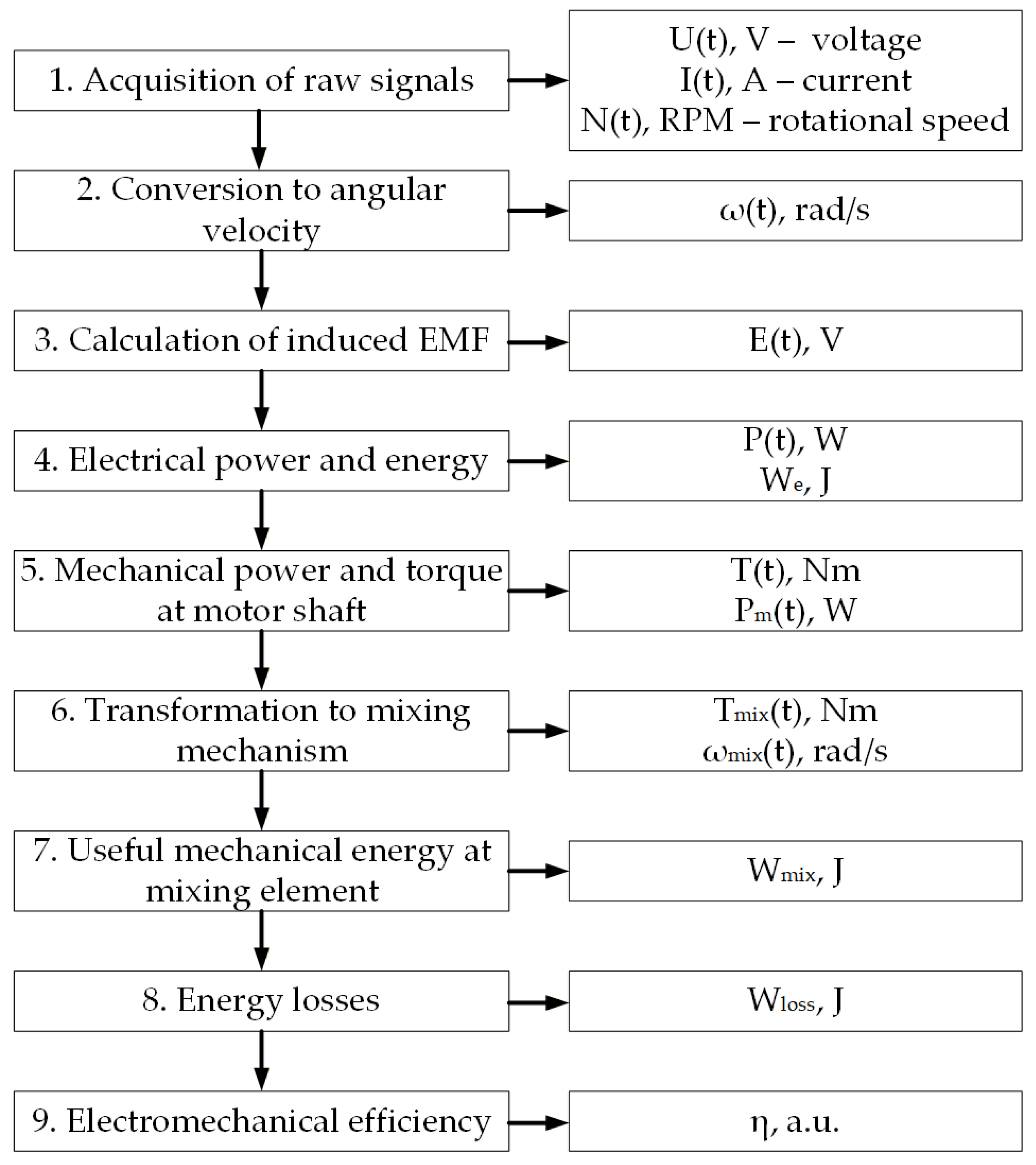
The computational workflow for deriving the electromechanical and viscoelastic characteristics of the bread-making system follows a sequential, dependency-based structure. The process is organized into nine stages, each using the outputs of the previous step to ensure consistency and avoid circular dependencies. The block diagram presented in Figure 4 summarizes the sequential workflow used to compute the electromechanical and viscoelastic characteristics of the bread-making system. It begins with the acquisition of raw electrical and mechanical signals and proceeds through the calculation of angular velocity, induced EMF, electrical power, torque, and mechanical power. The workflow then applies the belt-drive transformation to obtain the torque and speed at the mixing mechanism, which is followed by the computation of useful mechanical energy and energy losses. The final step evaluates the overall electromechanical efficiency. Each stage uses the outputs of the previous one, ensuring a clear, reproducible, and logically ordered computational process.

2.5. Selection of Informative Features

The RReliefF algorithm is a robust method for determining the weights of features describing studied objects. It is designed for regression tasks, extending the original ReliefF algorithm by assessing the relevance of features based on their ability to distinguish similar cases with different target values. RReliefF was used to assess the informativeness of each feature with a threshold weight of 0.6 being set as the criterion for selecting informative features. Features with weights exceeding this threshold were considered to have a significant impact on the target variable and were retained for subsequent modeling. This approach improves the interpretability of the model and reduces the dimensionality of the data while preserving their predictive power. The theoretical basis and empirical validation of RReliefF were reviewed by Robnik-Šikonja et al. [39] in their work on ReliefF-based algorithms for regression and classification tasks.
To assess the sensitivity of the selected features and their suitability for regression analysis, the k-fold, hold-out, and leave-one-out methods were applied [40,41,42]. By applying these approaches to different subsets of the data, it is checked to what extent the selected features retain their predictive ability when changing the training and test samples. The stable performance of the model in the different partitions shows which features are truly informative and contribute to increasing the accuracy and reliability of the regression models. The evaluation of the cross-validation results was made according to the criteria R2, SSE, RMSE, and MAE, which are presented as formulas in the subsection for regression models.

2.6. Reducing the Volume of Data in the Vectors of Selected Features

Principal component analysis (PCA) is a widely used data dimensionality reduction technique without training that transforms a set of possibly correlated variables into a smaller number of uncorrelated variables, which are called principal components. These components are linear combinations of the original variables and are ordered such that the first few retain most of the variation present in the original dataset. In this paper, PCA was applied to reduce the dimensionality of the data while preserving the structure of the variance, thereby increasing computational efficiency and interpretability. Features with high values of the weight coefficients on the first few principal components were considered informative and were retained for further analysis. This method is particularly effective in identifying latent patterns and eliminating redundancy in high-dimensional data. The theoretical foundations and practical applications of PCA are presented by Gewers et al. [43].
Prior to PCA, all variables (current, voltage, speed, torque, flour type) were standardized using z-score normalization. PCA was performed on the correlation matrix, and components with eigenvalues >1 (Kaiser criterion) and cumulative explained variance above 90% were retained. For all flour types, this resulted in 2 principal components.

2.7. Regression Method Used

The regression method used is a nonlinear regression. This approach allows to model the complex relationship between the reduced set of independent variables and the dependent variable. The regression form used is quadratic:
z = b 0 + b 1 x + b 2 y + b 3 x 2 + b 4 y 2 + b 5 x y
where x and y are the first two principal components (PC1 and PC2) and represent independent variables in the model; z is the dependent variable—torque; b represents the coefficients of the model.
The following were used to evaluate the model: coefficient of determination R2; Fisher’s exact test (F) compared to its critical value (Fcr); p-value; standard error (SE) [44].

2.8. Schematic Diagram for Simulation Analysis of an Electromechanical System with an AC Electric Motor and a Viscoelastic Load

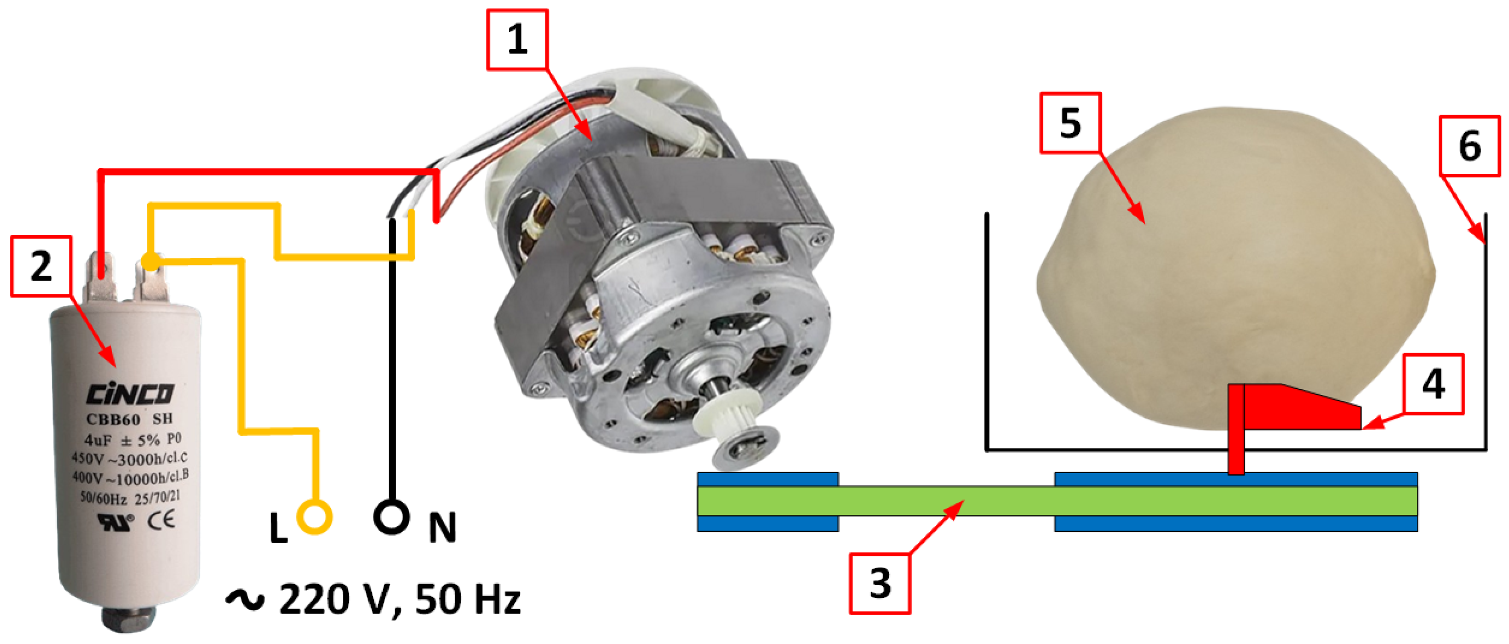
Figure A1 of Appendix A presents the schematic diagram of the experimental setup used for the simulation analysis. The electromechanical setup is a generalized model of a kneading system in an automatic bread machine, in which the individual elements are functionally connected without the need for designation by numbers or positions. At the base of the system is a single-phase asynchronous electric motor, to which a starting capacitor is connected, providing the necessary conditions for starting and stabilizing the torque. The resulting mechanical motion is transmitted to a belt drive, which adapts the speed and torque to the requirements of the subsequent mechanism.
After the transmission unit, a stirring mechanism is located, the kinematic structure of which is designed to provide the necessary deformation and movement regime of the processed material. This material is a visco-elastic load, which was modeled to describe the behavior of the dough during kneading. The entire process takes place in a kneading vessel, which limits the working space and determines the boundary conditions of interaction between the mechanism and the dough.
The combination of system-level modeling, flexibility in abstraction, and the ability to integrate real-world measurements makes MATLAB/Simulink (The MathWorks Inc., Natick, MA, USA) a suitable tool for analyzing the electromechanical system of an automatic bread machine. In this paper, simulations serve as a basis for calibrating the model against experimental data and for investigating the behavior of the system at different hydration levels. This task would be significantly more difficult and expensive to perform using physical experiments alone.

2.9. Software Products Used

For the processing of experimental data and the presentation of the results, the following software tools were used:
  • MS Office 2016 (Microsoft Corp., Redmond, WA, USA) was applied for the preparation of spreadsheet calculations and graphical presentations;
  • MATLAB 2017b (Mathworks Inc., Natick, MA, USA) was used as the main environment for numerical analysis, visualization and development of algorithms related to the simulation of the electromechanical system.
  • Additional statistical processing, modeling and creation of regression models were performed with Statistica 12 (TIBCO Software Inc., Palo Alto, CA, USA), which provides advanced capabilities for data analysis and graphical presentation.
  • Nextion Editor v.1.65.1 (ITEAD Intelligent Systems Co. Ltd., Shenzhen, China). The graphical interface of the touch screen display was developed with this application.

2.10. Comparative Analysis of the Results Obtained

The comparative analysis between the real electromechanical system of an automatic bread machine and the simulation model developed in MATLAB/Simulink and Simscape was performed by parallel measurement and the calculation of basic electrical and mechanical parameters. The experimental section includes recording the supply voltage, current, angular velocity and torque for different types of flour and hydration levels. The data were collected by integrated current, voltage and speed sensors, and the measurements were performed under real operating conditions of the machine.
The simulation model was configured to reproduce the same operating modes with identical input parameters set—supply voltage, rated motor power and mechanical load, which was modeled as a hydration-dependent visco-elastic element. In Simscape, the dynamic changes of torque, angular velocity, power factor and efficiency under different loads were tracked.
The real and simulated electromechanical systems are compared using a model of the following type:
y = a x + b
where y is the dependent variable; x is the independent variable; and a and b are the model coefficients.
To assess the correspondence between the real and simulated data, standard statistical indicators were calculated. The mean absolute error (MAE), the sum of squared errors (SSE), and the root mean square error (RMSE) were calculated using the following formulas:
M A E = 1 N i = 1 N y r y s
S S E = 1 N i = 1 N y r y s 2
R M S E = 1 N i = 1 N y r y s 2
where N is the number of measurements; yr represents the measurements from the real system; and ys represents the measurements obtained from simulation analysis. The coefficient of determination is derived directly from an MS Excel spreadsheet.
These metrics allow a quantitative comparison of the two systems and an assessment of the accuracy of the model. Additionally, comparative graphs for torque and angular velocity were constructed, which visualize the dynamic differences and similarities between the experimental and simulation results.
The methodological approach is compared with the available literature, which emphasizes the importance of the rheological properties of the dough and their influence on the mechanical loads of the electromechanical system.
All data were processed at a significance level of α = 0.05.

3. Results and Discussion

3.1. Simulation Analysis of Electromechanical Control System of Automatic Bread Machine

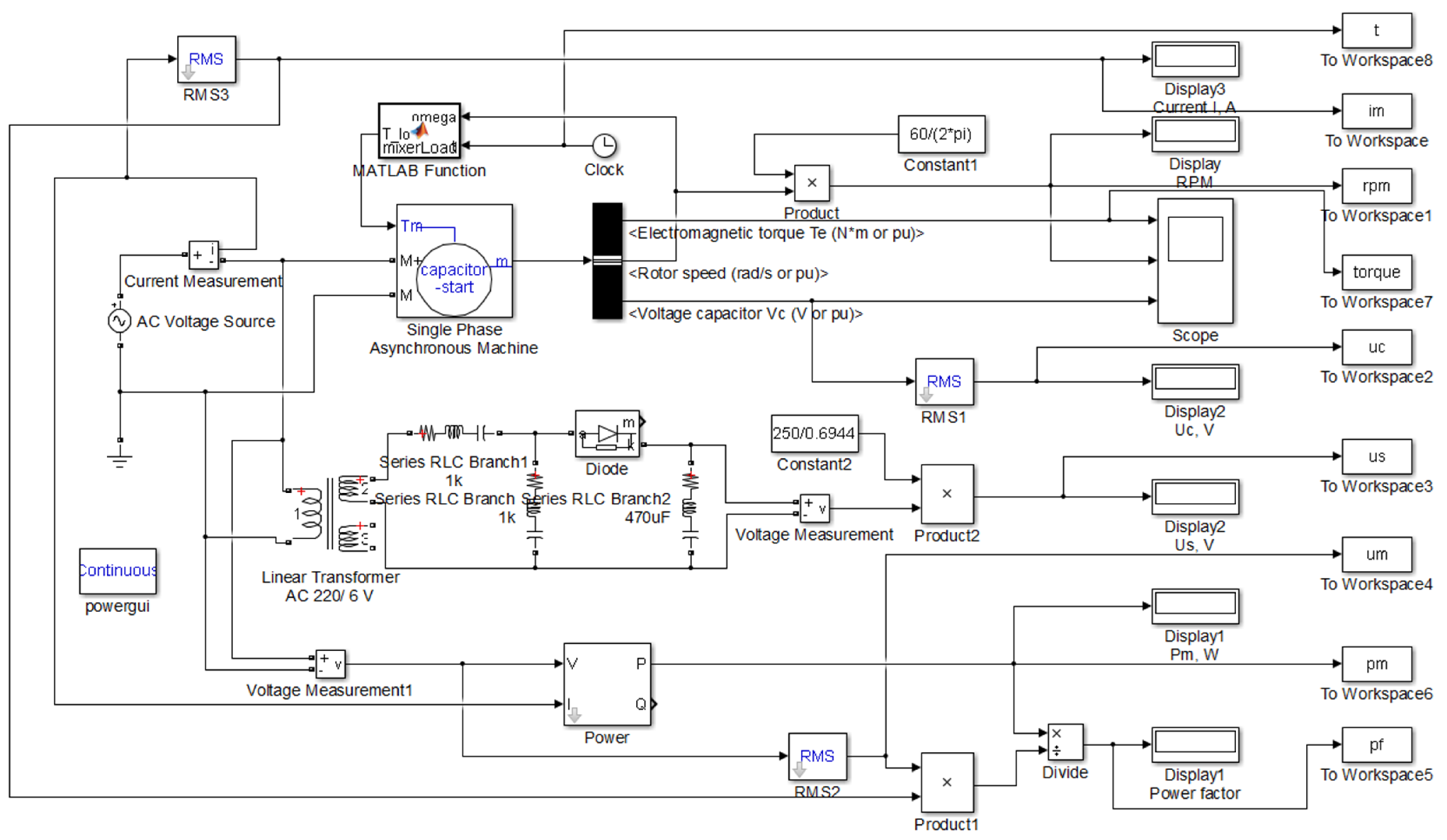
Figure 5 shows the simulation diagram of an electromechanical system with a viscoelastic load. It includes a single-phase induction motor with a starting capacitor, driven by an AC source, which is connected to a viscoelastic load, which is simulated by a Matlab function block. In order to measure and monitor the operation of the system, multiple measuring instruments are integrated that measure current, voltage, power and power factor, as well as a voltage sensor that converts the input voltage to a lower value suitable for measurement. The simulation results are analyzed and recorded using the Display, Scope and To Workspace blocks, which allow both visual observation and subsequent analysis of parameters such as torque, speed and power factor.
Appendix A, Figure A2 presents the configuration of the electric motor model together with the functional block used for generating the viscoelastic load in the electromechanical simulation.
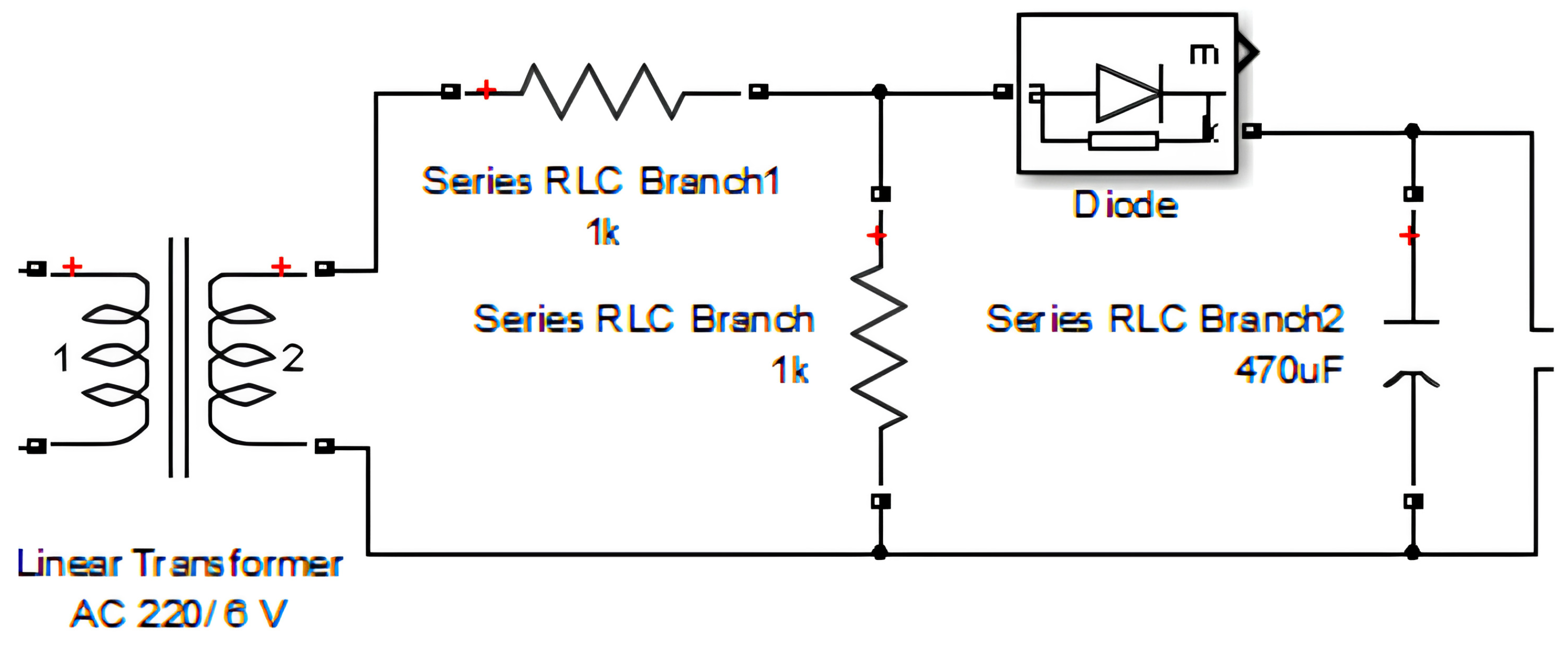
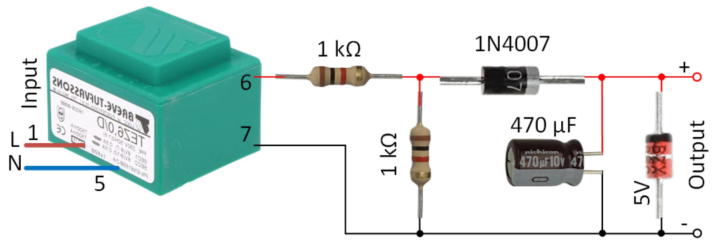
Figure 6 shows a simulation circuit of a voltage sensor. The voltage of 311 V AC is reduced to 6 V AC by a transformer. A voltage divider with 1 kΩ resistors is used. The rectifier diode cuts off the lower half-wave of the sinusoidal signal. The 470 µF capacitor smooths the resulting voltage signal.
Table 3 describes the viscoelastic load (bread dough) of the electromechanical system. These are approximate values based on typical resistances when kneading dough with a humidity of about 60–65%. The direct relationship between the mass of the dough and the required torque is presented, which is the main indicator of the load on the electric motor. Different load levels are shown-from minimal (580 g of dough) to limit (1050 g of dough), which requires sufficiently powerful electric motors that are typical of professional models of automatic bread machines. Accordingly, for each gram of dough, the final gram of the baked bread is also indicated, ranging from 580 g (individual) to 1050 g (for professional use or “batch bread”). Increasing the mass of the dough leads to a higher load on the mechanism, and this corresponds to the different sizes of bread.
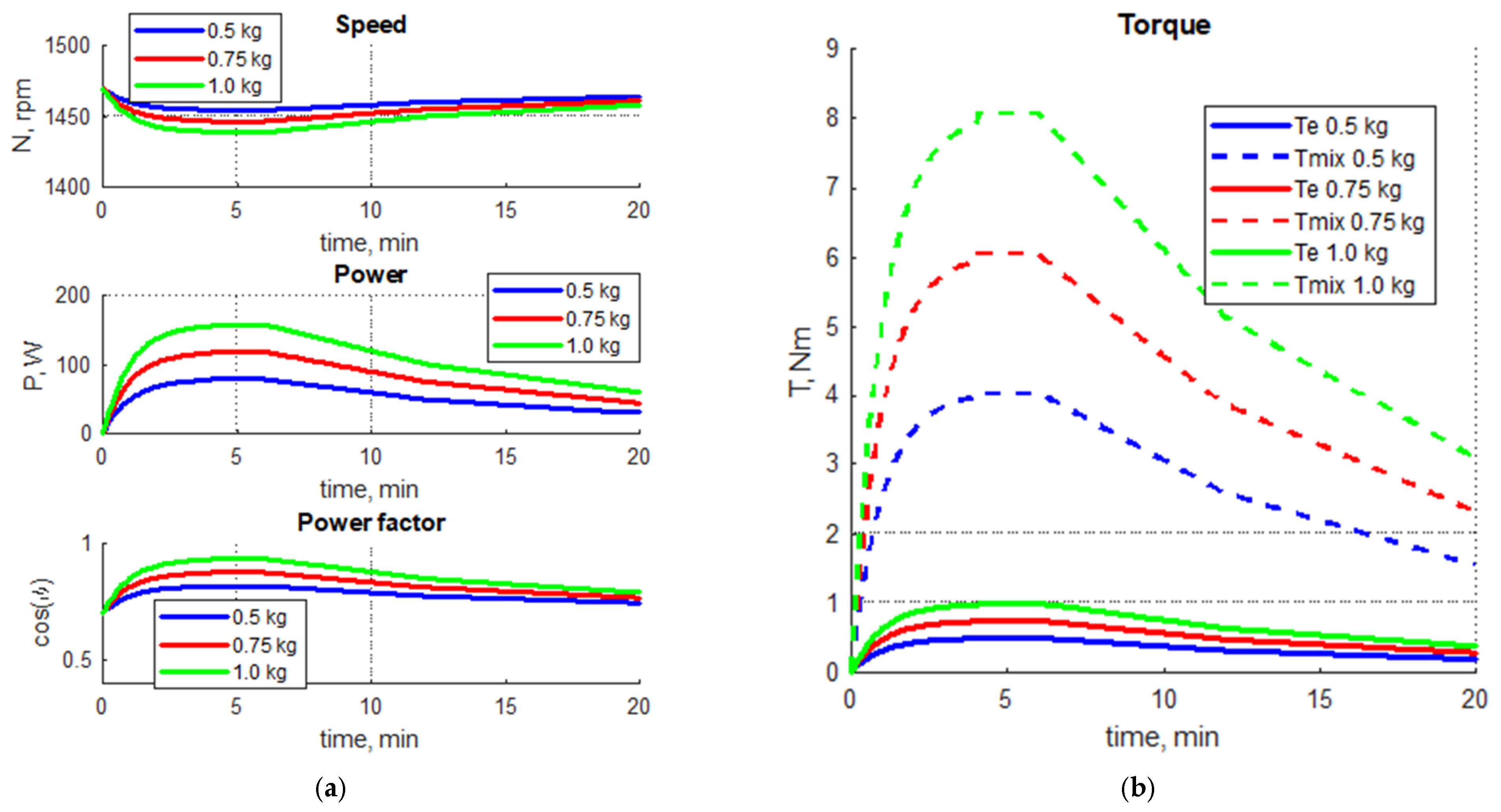
Figure 7 shows the results of a simulation of the load on the electric motor. The increase in the mass of the dough, which acts as a viscoelastic load, has a direct impact on the operation of the electric motor of the automatic bread machine. As the mass of the dough increases, both the required mechanical power and the power factor increase. This means that the motor operates under a greater load and more efficiently uses the electrical energy to overcome the resistance of the larger mass of the dough. Despite the increased load, the rotor speed is maintained in a relatively constant range, which indicates the ability of the system to cope with different loads, ranging from light to maximum, which is typical of professional machine models. As the mass of the dough increases, the required mechanical power increases. At lower weights, the motor operates at lower power, while at large masses (900 g and 1050 g), the peak power reaches its highest values since more energy is required to knead the denser and larger amount of dough are required as well. As the load increases (i.e., with a larger dough mass), the power factor increases, approaching 0.95. This indicates that the motor is working more efficiently and converting a larger part of the energy consumed into useful mechanical work. Although the load increases, the rotor speed remains relatively constant. Slight fluctuations and dips are observed at peak load moments, but these are minimal.
The torque of the electric motor is constant and always lower than that of the load (dough) to ensure continuous and efficient mixing. As the dough mass increases, the base torque provided by the electric motor also increases to compensate for the greater resistance. In turn, the torque of the load (dough) is dynamic, being highest at the beginning of the mixing process and gradually decreasing as the gluten network softens and develops. This relationship shows that the motor provides the required torque, which varies depending on the amount of dough, while ensuring that the load resistance does not exceed the capabilities of the system within the range of dough mass variation.
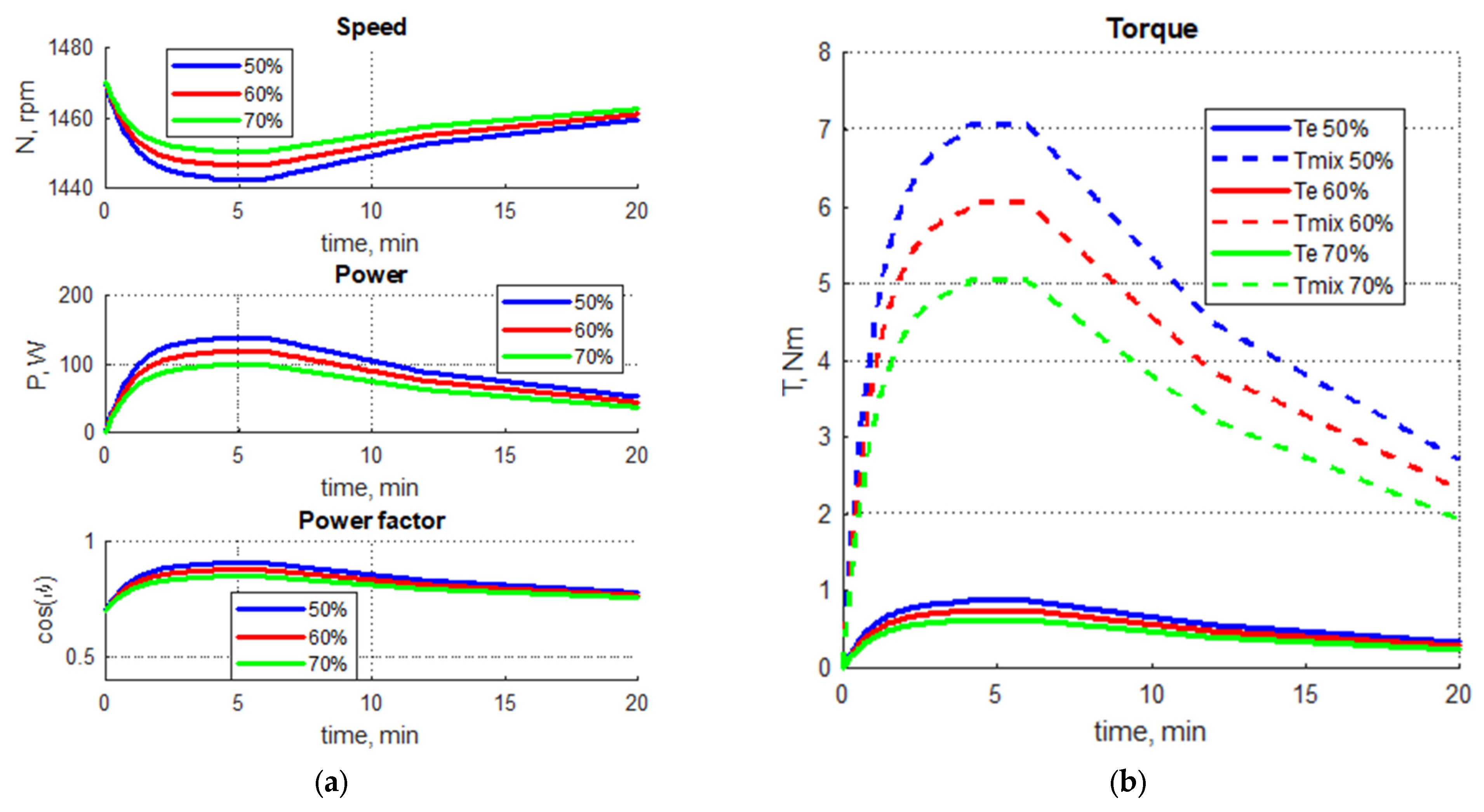
A simulation was made for changing the amount of water in a dough with a mass of 500 g. The amount of water is 50%, 60% and 70%. This change was made by changing the values of b and T_step for each amount of water in the dough in the code of the load simulation function (Table 4).
Figure 8 shows the results of the simulation of the operation of the electromechanical system when changing the amount of water in a viscoelastic load (dough). The amount of water in the dough has a direct impact on the operation of the electromechanical system of the automatic bread machine. As can be seen from the graphs, less water (50%) leads to a denser and stiffer dough, which requires higher torque and mechanical power from the electric motor. A larger amount of water (70%) creates a softer dough, which requires lower torque and power from the electric motor. Despite these differences in load, the rotor speed remains relatively constant for all three cases. The power factor remains close to 0.8.
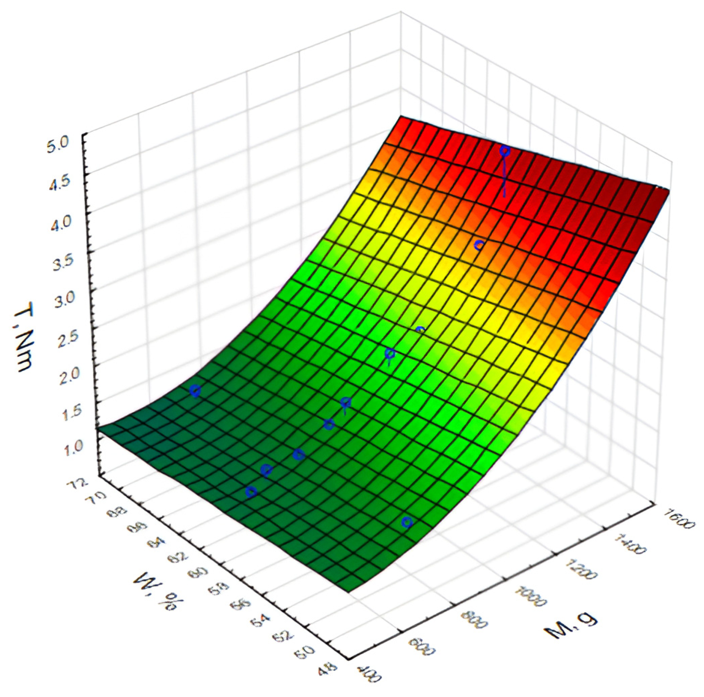
From the results obtained so far, a regression model can be created describing the relationship between two independent variables, dough mass and water quantity, and the dependent variable—electric motor torque.
After removing the insignificant coefficients with p > α, we have a model of the form
T = 1.6 + 0.000002 M 2 0.000027 M W
where T is the torque of the load, which is measured in Nm; M is the mass of the dough, which is measured in g; and W is the percentage of water in the dough.
The coefficient of determination for the model is R2 = 0.96. According to the Fisher criterion F(2, 8) = 110 >> Fcr = 4.46. The standard error is SE = 0.19. The analysis of the residuals showed that they are close to the normal probability plot, and their distribution is close to normal. According to these evaluation criteria, the obtained regression model is adequate and describes the experimental data with sufficient accuracy.
In general graphical form, the obtained regression model is presented in Figure 9. The torque of the electric motor is highest when the dough is dense (low percentage of water) and its mass is relatively high. The torque is lowest for softer dough (high percentage of water) and low mass. The resulting regression model can be used to predict the required torque under different operating conditions of an automatic bread machine.

3.2. Development of a Control System for the Electromechanical System of an Automatic Bread Machine

Figure 10 shows a developed control system for the electromechanical system of an automatic bread machine. The Mega 2560 single-board microcomputer receives input signals from the temperature sensor, the RPM sensor, the voltage sensor and the current sensor. Based on these data, the microcontroller controls the heater and the motor through the TRIAC switches. The user interacts with the system through the Nextion display, where the measurements are visualized. The pointer ammeter and voltmeter display additional information about the electrical parameters current and voltage.
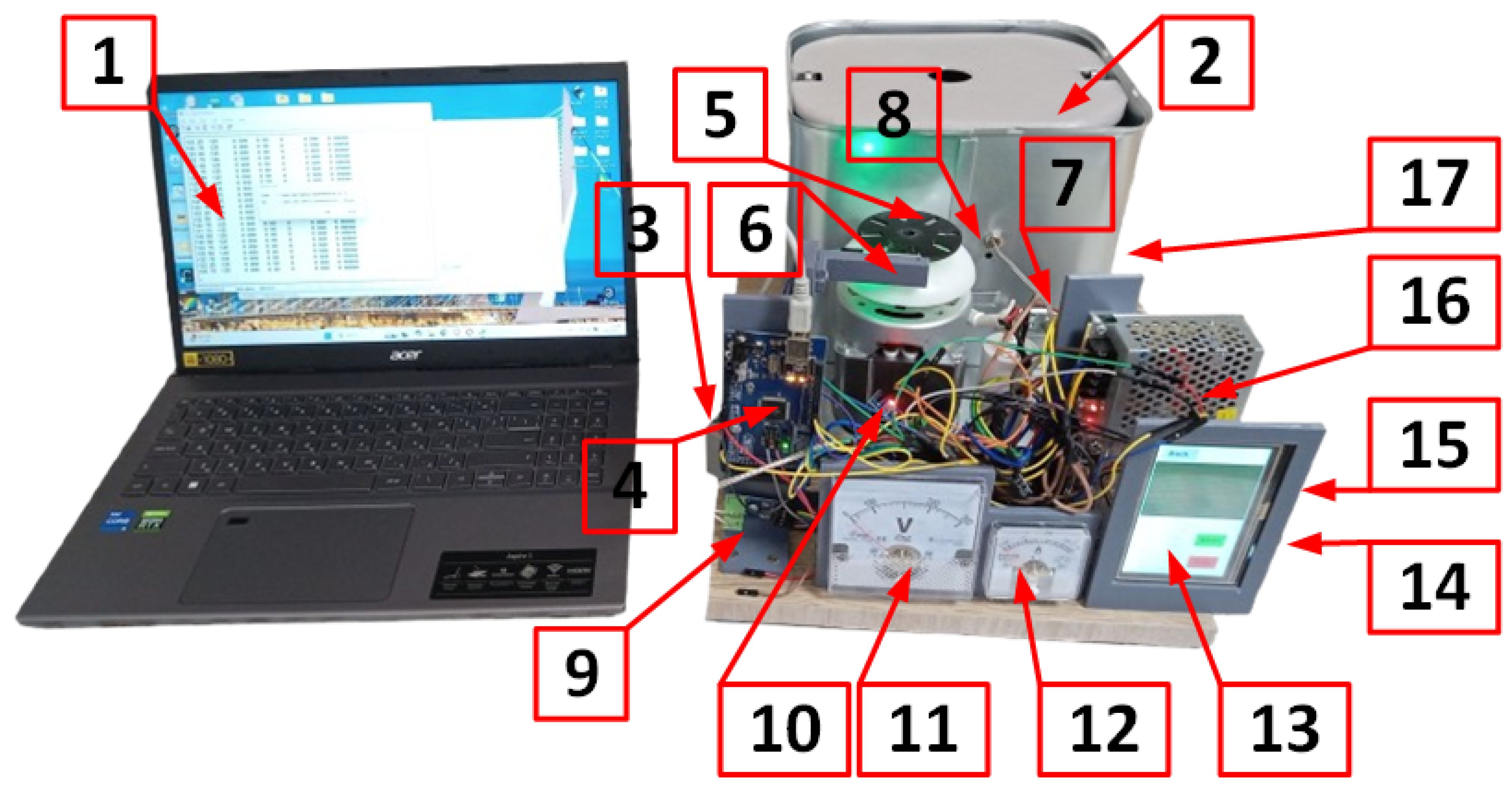
Figure 11 shows in general form the experimental setup for determining the characteristics of an electromechanical system for dough preparation. Position 1 indicates the personal computer on which the data used in the analysis of the electromechanical system are recorded. Position 2 represents a vessel with a stirring element. The voltage sensor is marked with 3, and the single-board microcomputer is marked with 4. The schematic diagram and description of the voltage sensor are presented in Appendix A (Table A2 and Figure A3). The electric motor with a mounted measuring disk with holes is marked with 5, and the speed sensor is marked with 6. The heater is marked with 7, the thermocouple with 8, and its sensor-amplifier with 9. The current sensor is at position 10, the analog voltmeter is at position 11, and the analog ammeter is at position 12. The display is marked with 13. The solid state relays (SSRs) for controlling the heater and the motor are at positions 14 and 15, respectively. The power supply unit is marked with 16, and the belt drive located under the dough container is marked with 17. Video of the system is presented in Supplementary Materials.
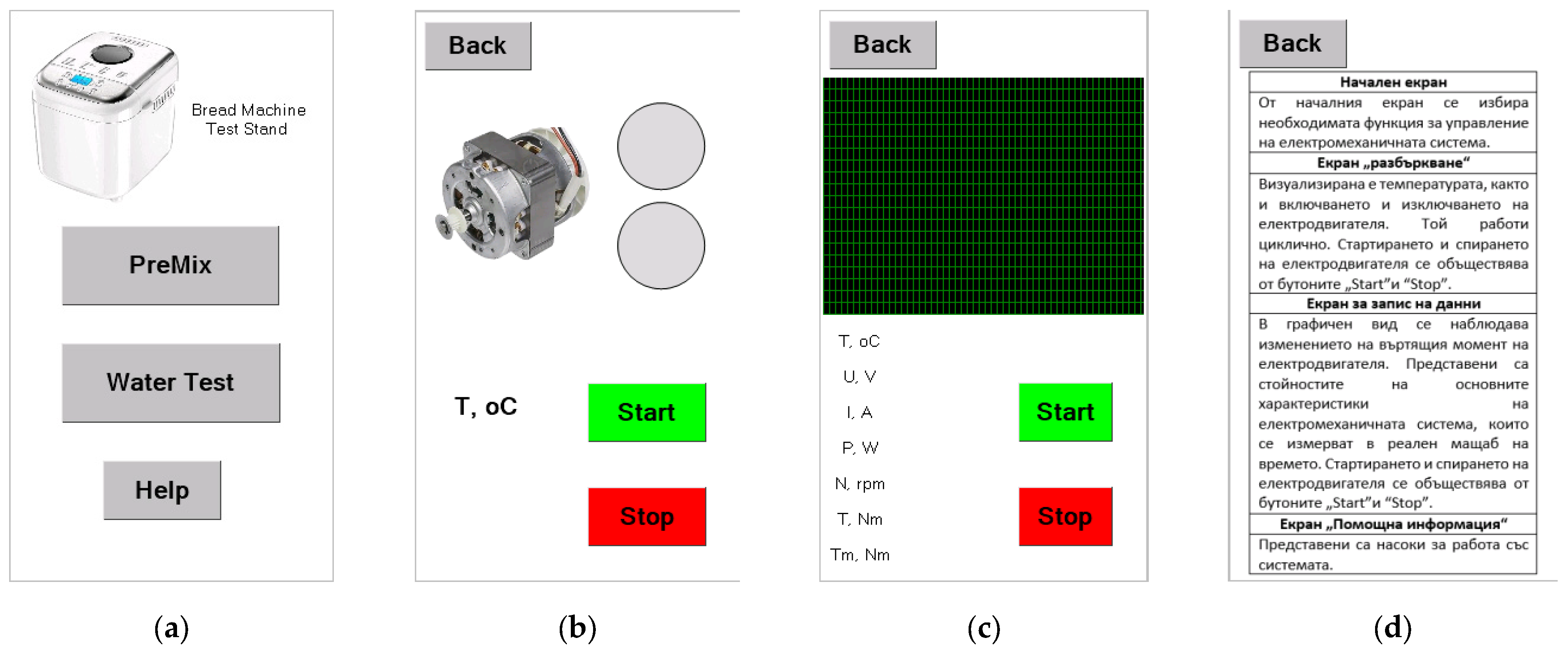
The developed algorithm, subroutines, graphical user interface and setup of the PID controller are presented in Appendix A (Table A3, Table A4 and Table A5; Figure A4, Figure A5, Figure A6 and Figure A7).

3.3. Results of Kneading Dough with Different Amounts of Water

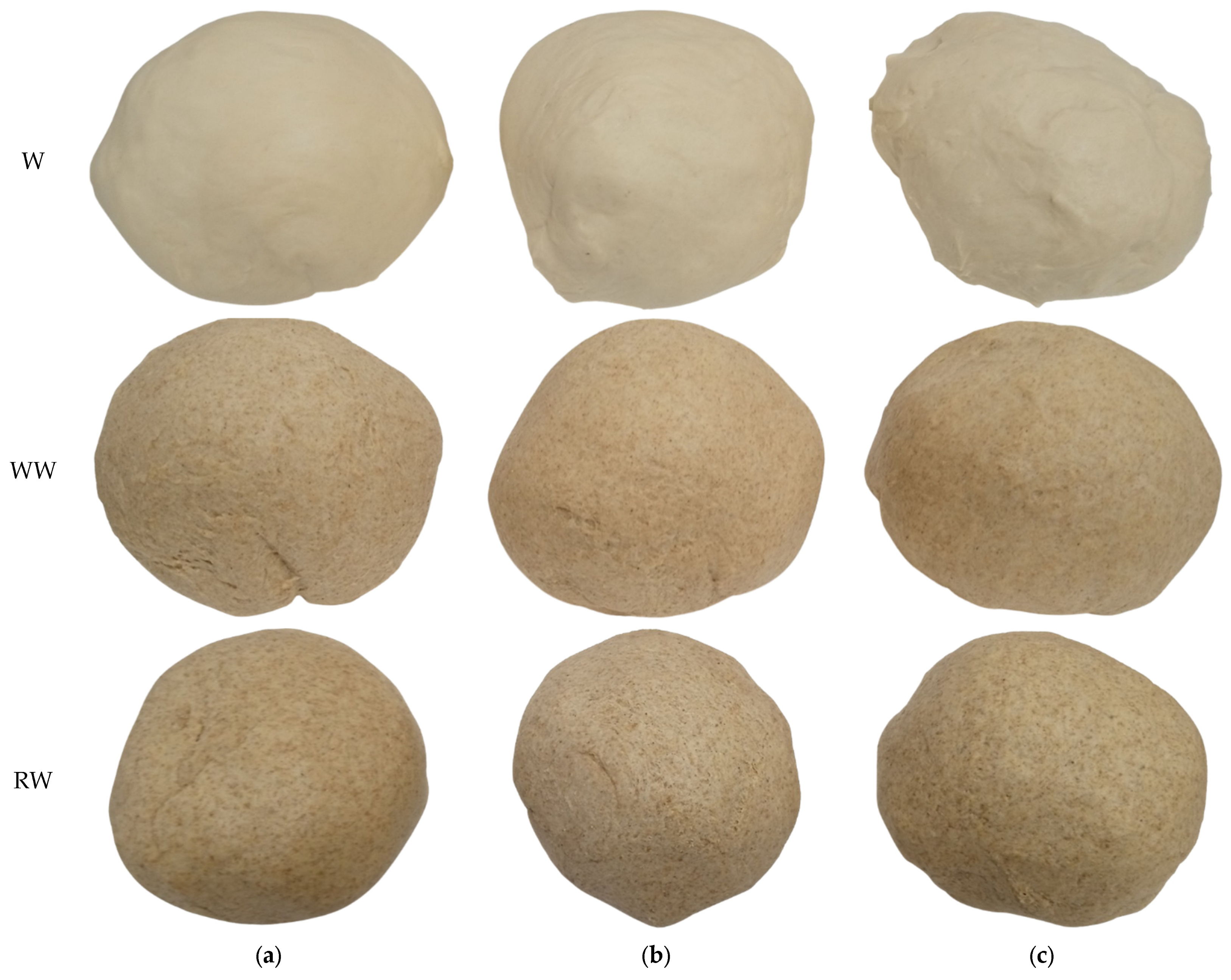
In general, the dough prepared in an automatic bread machine with an electromechanical system is presented in Figure A8 in Appendix A. The three types of dough used in the study are shown—type 500 flour, type 1850 wholemeal flour and rye–wheat flour—each at different levels of hydration. The amount of water determines the rheological properties of the dough, including its elasticity, plasticity, viscosity and ability to deform under mechanical load, which directly affects the torque recorded by the electromechanical system.

3.4. Determining Electrical and Mechanical Characteristics of an AC Motor

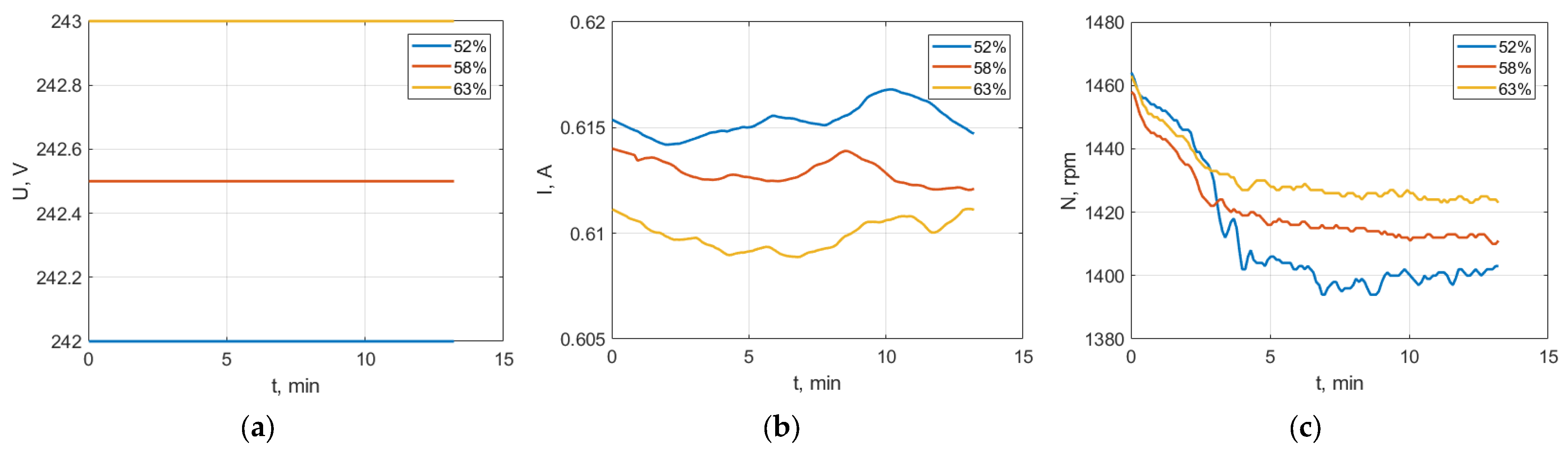
Figure 12 shows graphs of voltage, current and speed in rpm of the electric motor of an automatic bread machine when kneading dough from type 500 flour and different amounts of water. At 52% water, the dough is the densest, which leads to high mechanical resistance. This is reflected in an increase in the values of the current (I) and reduced revolutions (N) of the motor, while the voltage (U) remains relatively stable but with distinct fluctuations in the initial phase. At 58% water, the dough reaches optimal consistency—t he current stabilizes, the revolutions increase, and the voltage is smoothed out, which indicates an efficient and balanced operation of the system. At 63% water, the dough is soft and easy to process—the current has the lowest value, the revolutions are the highest, and the voltage is the most stable, but too low a load can lead to insufficient structuring of the dough. These dependencies confirm that 58% water provides a relatively good compromise between energy efficiency and technological stability.
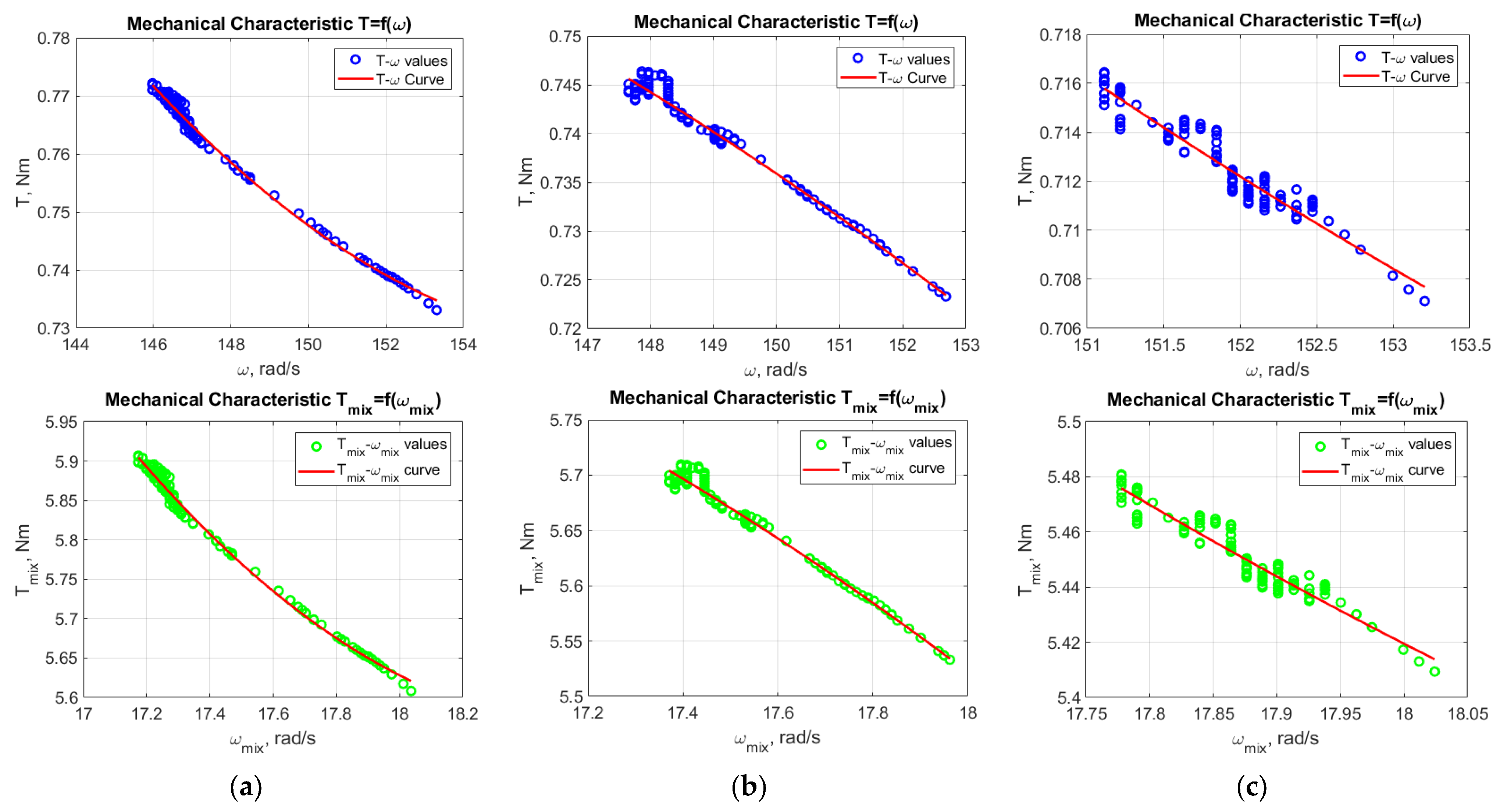
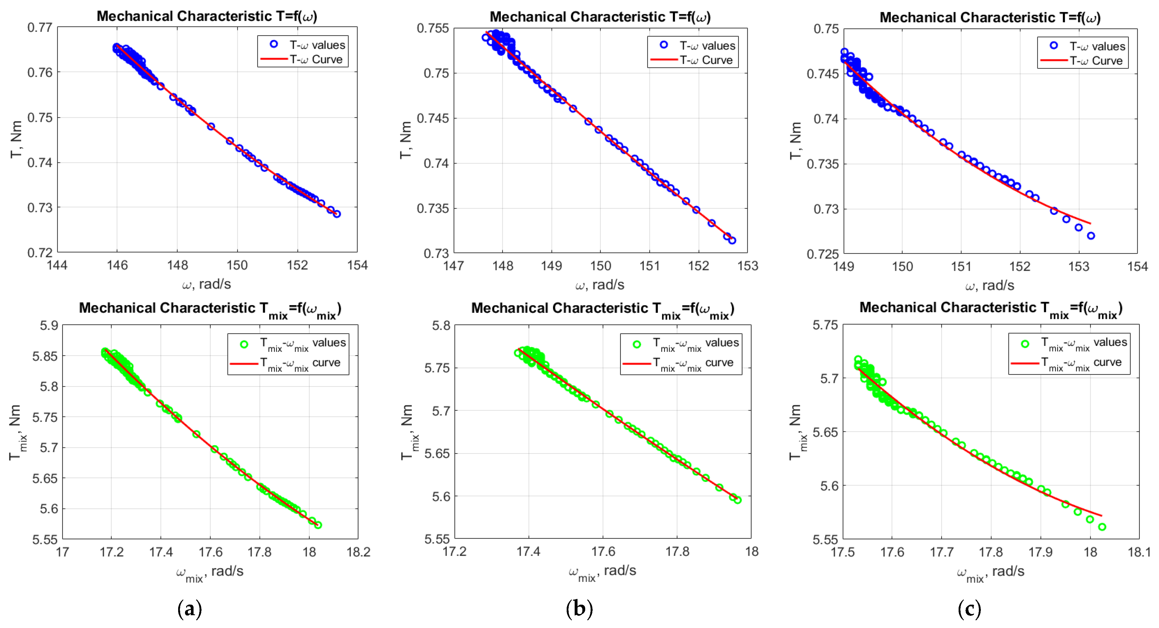
Figure 13 shows graphs of the function T = f(ω) of the electric motor and the stirring mechanism for a load of type 500 flour dough. The study of the relationship between the torque (T) and the angular velocity (ω) when kneading dough with different water contents (52%, 58% and 63%) shows a clearly expressed mechanical characteristic of the electric motor and the stirring mechanism. In all cases, the typical inversely proportional relationship is observed—with increasing angular velocity, the torque decreases. For dough with the lowest water content (52%), the torque is highest at low values of the angular velocity, which suggests that the motor must overcome greater resistance in the harder dough (with lower hydration). At lower humidity (52%), both components are subjected to higher mechanical resistance—the motor requires more force, and the mechanism generates greater torque. With increasing water to 63%, the load decreases significantly, which facilitates dough mixing, but it may compromise the technological result. The most balanced characteristics are observed at 58% water, where the system operates with optimal efficiency and stability.
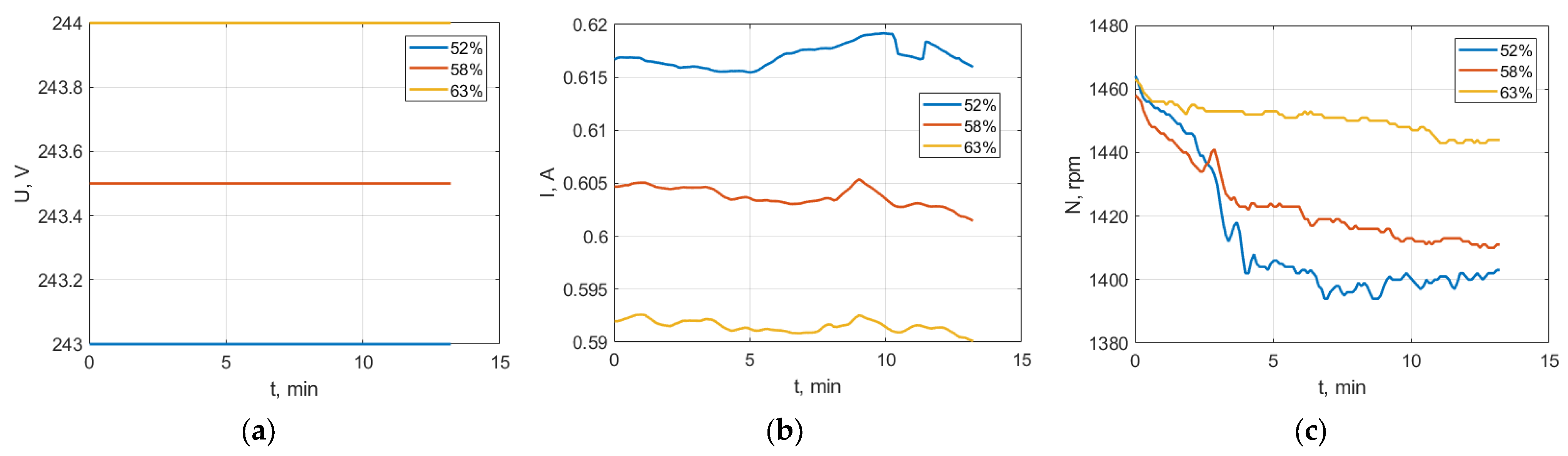
Figure 14 shows graphs plotting the voltage, current and speed of the electric motor of an automatic bread machine when kneading dough from type 1850 flour and different amounts of water. When kneading dough with type 1850 flour in an automatic bread machine, the electric motor shows clearly pronounced changes in its electrical characteristics depending on the water content. At 52% water, the voltage and current are the highest, and the revolutions are lower and unstable, which reflects the high mechanical resistance of the thick dough. At 58% water, the parameters stabilize—the voltage and current decrease moderately, and the revolutions approach the nominal ones, which indicates optimal load and good workability. At 63% water, the dough is soft, the resistance is minimal, the current and voltage are the lowest, and the revolutions are the highest.
Figure 15 shows graphs of the function T = f(ω) of the electric motor and the stirring mechanism for a load of wholemeal flour dough type 1850. The mechanical characteristic, expressed by the dependence between the torque (T) and the angular velocity (ω), shows the typical hyperbolic shape, in which the torque decreases with increasing revolutions. This behavior is common to all studied dough hydrations, but some differences are observed in the scale and slope of the curves depending on the water content. At 52% water, the highest torque is observed, which indicates significant resistance and difficulty in mixing. At 58%, the torque stabilizes, which suggests better workability and energy efficiency. At 63% water, the resistance is minimal, but too soft dough can lead to technological problems with the resulting product. The water content of 58% again emerges as optimal for the balanced operation of the mechanism.
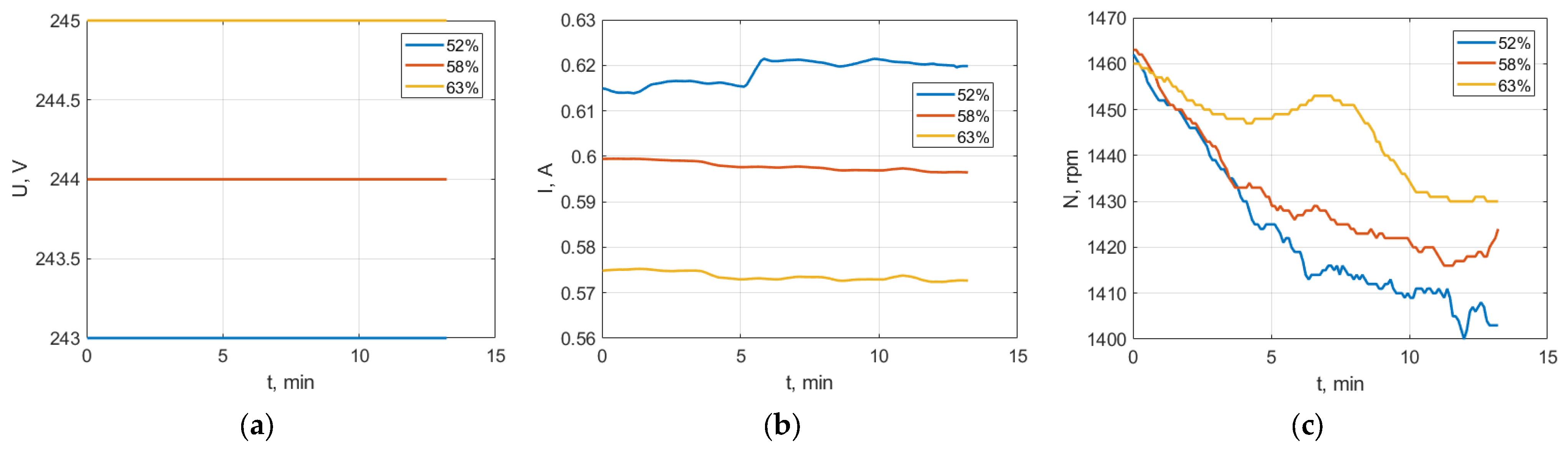
Figure 16 shows graphs plotting the voltage, current and speed of the electric motor of an automatic bread machine when kneading dough from rye–wheat flour and different amounts of water.
When kneading dough with rye–wheat flour in an automatic bread machine, the electric motor shows clearly pronounced changes in its electrical parameters according to the water content. At 52% water, the current is highest and the revolutions are lowest, which reflects significant mechanical resistance and load. At a water content of 58%, the current stabilizes, the revolutions increase, and the voltage remains stable, which indicates a balanced and efficient operation of the system. At 63% water, the lowest current consumption, highest revolutions, and smoothest voltage profile are observed. The best electromechanical stability is observed at 58% water.
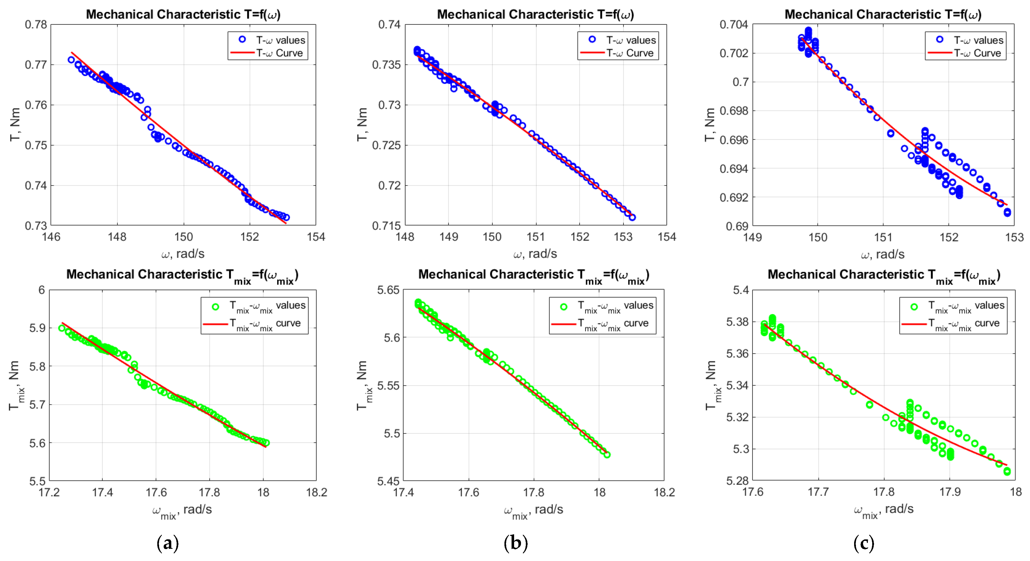
Figure 17 shows graphs of the function T = f(ω) of the electric motor and the stirring mechanism for a load of rye–wheat flour dough. The mechanical dependence between the torque (T) and angular velocity (ω) at the three hydration levels (52%, 58% and 63%) follows the expected trend—with increasing speed, the torque decreases.
At 52% water, the highest torque is observed, which indicates significant resistance and difficulty in processing. At 58%, the torque stabilizes, and the curve shows smoother behavior—a sign of optimal processability. At 63% water, the resistance is lowest, but too soft dough can lead to technological deviations. Here too, the water content of 58% emerges as the most balanced for effective and stable operation of the mechanism.
It can be summarized that different types of flour (type 500, whole wheat type 1850 and rye–wheat) react differently to hydration, which directly affects the texture, elasticity and quality of the dough. Lower hydration leads to a denser and harder dough, while higher hydration creates a softer, stickier and airier dough, especially with type 500 flour. Whole wheat and rye–wheat dough absorb more water, leading to a weaker gluten network. These differences in the structure and behavior of the dough place demands on the electromechanical control system of the automatic bread machine—it must provide precise control of the kneading, time and temperature according to the specific type of dough and hydration level.

3.5. Operating Points of the Electromechanical System with an AC Electric Motor for Different Types of Flour and Hydration Levels

The operating points of the electromechanical system with an AC electric motor are determined for three types of flour—white, whole grain, and rye–wheat, at three levels of hydration—52%, 58%, and 63%. For each combination, the average values of the angular velocity and torque of the electric motor were calculated as well as the corresponding values after the belt drive that drives the stirring element. The results obtained allow us to assess the influence of the rheological properties of the dough on the load of the electromechanical system and to analyze the adaptability of the motor to different technological conditions. The results of this analysis are presented in Table 5.
Regardless of the type of flour, increasing hydration leads to a pronounced tendency to reduce the torque and slightly increase the angular velocity. At lower hydration (52%), the dough is stiffer and offers greater resistance to the mixing mechanism, which leads to higher torque values, both of the motor (T ≈ 0.45–0.51 Nm) and of the mixing element after the gear (Tmix ≈ 3.8–4.4 Nm). At higher hydration (63%), the dough becomes softer and easier to process, which reduces the load on the system. In this case, the torque of the electric motor drops to 0.28–0.40 Nm, and the torque of the mixing element drops to 2.36–3.41 Nm. This also leads to an increase in the angular velocity of both the motor (ω ≈ 149–152 rad/s) and the mixing element (ωmix ≈ 17.6–17.9 rad/s).
The comparison between the different types of flour shows differences in the load on the system. Wholemeal flour leads to the highest torque values at low hydration (Tmix ≈ 4.37 Nm at 52%), which is due to the higher fiber content and greater water absorption of the flour. At the same time, it also demonstrates the strongest torque drop with increasing hydration to only 2.36 Nm at 63%, which indicates a high sensitivity of its rheological properties to the amount of water. White flour exhibits the most balanced behavior with moderate torque values and a smooth change at different hydrations. Rye–wheat flour occupies an intermediate position—at 52% water, the load is lower than that of wholemeal but higher than that of white, and at 63% water, the torque decreases to about 2.5 Nm.
In all cases, the asynchronous electric motor operates in a stable zone with little slip with its speed remaining in a narrow range around the nominal value (147.9–151.9 rad/s). This shows a sufficiently good adaptability of the electromechanical system to different loads without the risk of overload or instability. The belt drive provides the necessary increase in torque, amplifying the motor torque by approximately 8.5 times, which allows for the effective mixing of dough with different consistencies.
The results obtained show that hydration is one of the main factors determining the load on the electromechanical system. Harder doughs at low hydration lead to higher torques and lower revolutions, while softer doughs at high hydration reduce the load and allow for higher mixing speeds. The differences between flour types show the importance of their rheological properties for the operation of the system with wholemeal flour proving to be the most demanding on the motor at low hydration and white flour being the most balanced in a wide range of technological conditions.

3.6. Energy Analysis of the Electromechanical System of an Automatic Bread Machine When Kneading Dough with Different Compositions

The results in Table 6 show that the efficiency of the electromechanical system remains nearly constant across all flour types and hydration levels with values close to η ≈ 0.67 for every tested condition. The power factor also shows no systematic variation and stays around cos(φ) ≈ 0.85, indicating similar reactive characteristics of the load regardless of flour composition or water content. The electrical energy consumption (We) is highest for rye–wheat dough at 52% hydration (We ≈ 118,945 J), which is followed closely by whole-wheat (≈118,657 J) and white flour (≈117,850 J). For all flour types, increasing hydration from 52% to 63% leads to a gradual decrease in both electrical energy (We) and losses (Wloss), reflecting the lower mechanical resistance of more hydrated doughs. Among the tested conditions, whole-wheat dough at 63% hydration shows one of the lowest energy consumptions (We ≈ 114,223 J) and reduced losses (Wloss ≈ 37,122 J), indicating easier processing at higher hydration levels.
It can be summarized that the least load and energy losses are observed when kneading dough with white flour and/or high water content. Wholemeal flour creates the highest resistance in the mechanism and leads to maximum load on the electric motor. Regardless of external conditions, the system shows relatively constant efficiency, which is important for its long-term reliability and low energy consumption.

3.7. Determining the Amount of Water at Which the Electromechanical System of an Automatic Bread Machine Will Operate Efficiently Enough

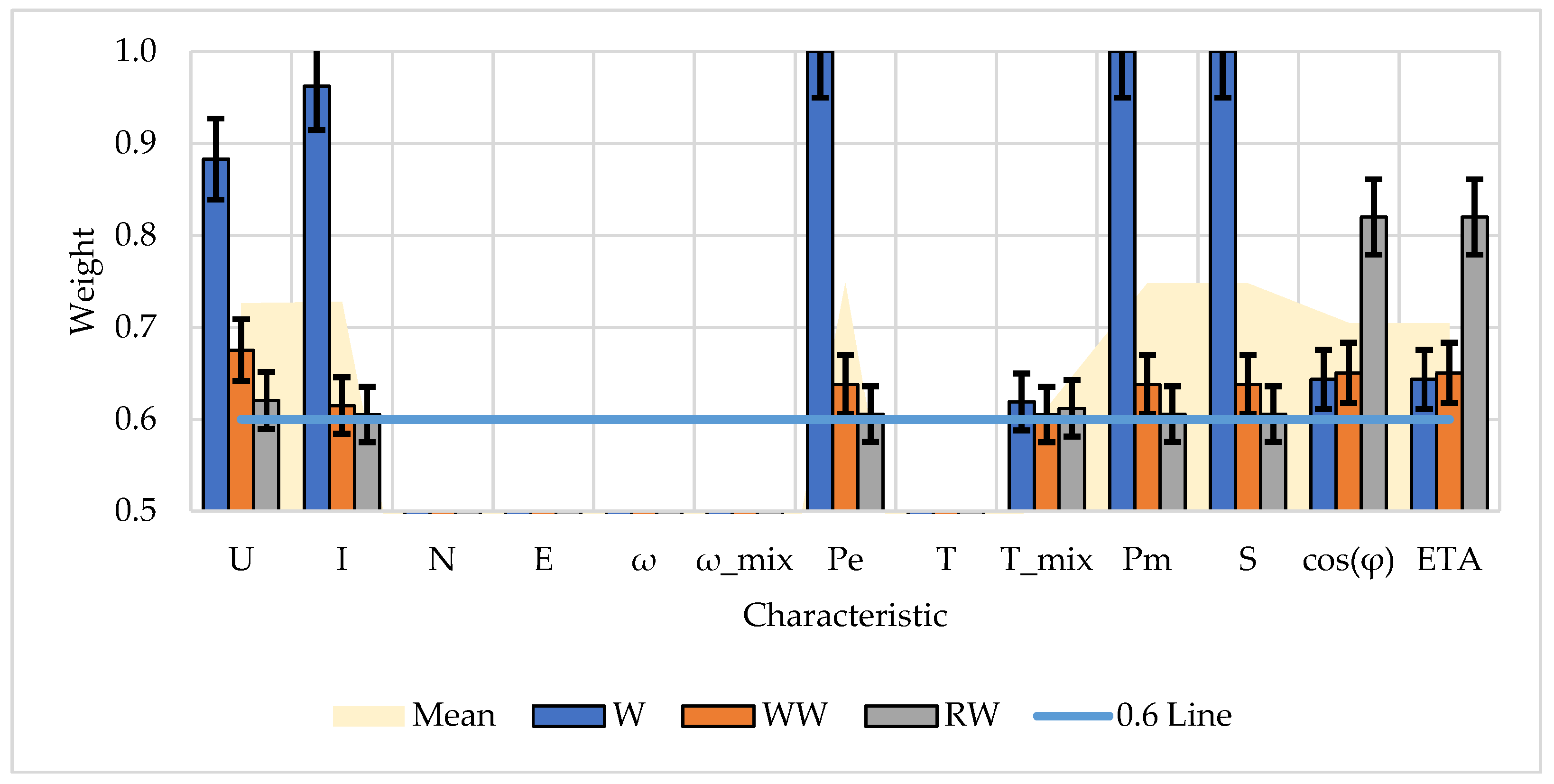
Figure 18 shows the results of selection of informative features. Those features were selected that have weight coefficients above 0.6. It can be noted that in all types of tests, the selected features are of the same type. Out of a total of 13 features, almost half (8) were selected. With the highest values of the weight coefficients, compared to all features, are those for the power of the electric motor and those of the mixing mechanism.
Table 7 presents the results of the verification of the selected features using four different cross-validation methods: k-fold, hold-out, leave-one-out, and repeated hold-out. For each method, the main criteria for evaluating the regression models (RMSE, MAE, SSE, and R2) were calculated, which reflect the accuracy and stability of the predictions. The results show that all methods give close error values, which is an indicator of model stability and good informativeness of the selected features. The leave-one-out method achieves the lowest error (RMSE = 0.46; MAE = 0.38) and the highest explained variance (R2 = 0.88), which is expected due to the maximum use of the available data. K-fold (10) gives similar results (R2 = 0.87), while hold-out (70/30) shows higher errors (RMSE = 0.52), which is due to its dependence on a single data split. The R2 values in the range of 0.85–0.88 confirm that the selected features are suitable for regression modeling, and the error rates demonstrate good predictability and limited variability between different validation methods.
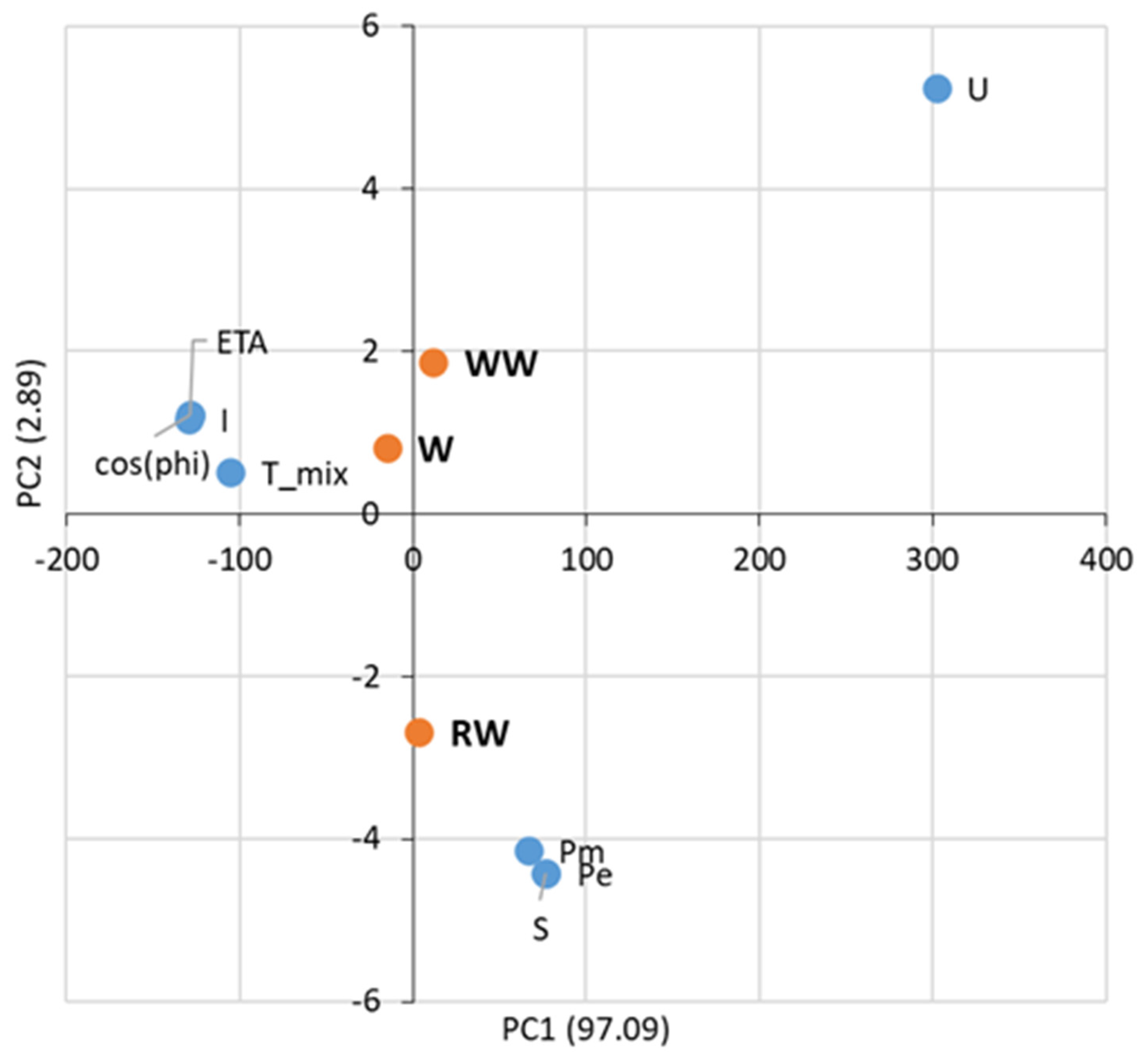
Figure 19 presents the results of the principal component analysis, where the original set of eight electromechanical features is reduced to two principal components. Together, PC1 and PC2 explain more than 90% of the variance in the experimental data, indicating that the main dynamic behavior of the system can be represented in a low-dimensional space.
PC1 captures the dominant variation in the electromechanical response. High positive loadings on voltage, electrical power and mechanical power suggest that this component reflects the overall energy demand of the system. The negative loadings on variables such as power factor, efficiency and torque indicate that PC1 also incorporates aspects of mechanical resistance. Thus, PC1 can be interpreted as an axis associated with the combined electrical–mechanical load experienced by the machine.
PC2 describes secondary variations that are not directly related to the main load axis. Its mixed positive and negative loadings indicate that it captures differences in the electrical dynamics of the system under similar mechanical conditions, such as variations in instantaneous current–voltage behavior.
The distribution of the three flour types in the PCA space follows these tendencies. White flour samples cluster near the origin, indicating stable and balanced electromechanical behavior. Wholemeal flour tends to occupy regions with higher PC1 values, reflecting increased mechanical resistance. Rye–wheat flour forms a separate cluster along PC2, suggesting distinct electrical characteristics associated with its specific dough structure.

3.8. Comparative Analysis of the Results Obtained

Table 8 presents a comparative analysis between the real (experimental) electromechanical system of an automatic bread machine and its simulation equivalent, which was implemented in the MATLAB/Simulink and Simscape environments. The comparison covers basic electrical and mechanical parameters, including supply voltage, rated power, torque, angular velocity, power factor, efficiency, and maximum torque. The data show that the simulated system reproduces the main trends observed in experimental measurements, such as the dependence between the load and the dynamic characteristics of the motor. However, differences are observed in the absolute values of the torque and speed, which is due to the idealized parameters in the model and the simplified description of the visco-elastic load. Despite these deviations, the simulation model demonstrates a high degree of correspondence (R2 = 0.64–0.96) and is suitable for the analysis, optimization, and prediction of the system behavior under different load regimes.
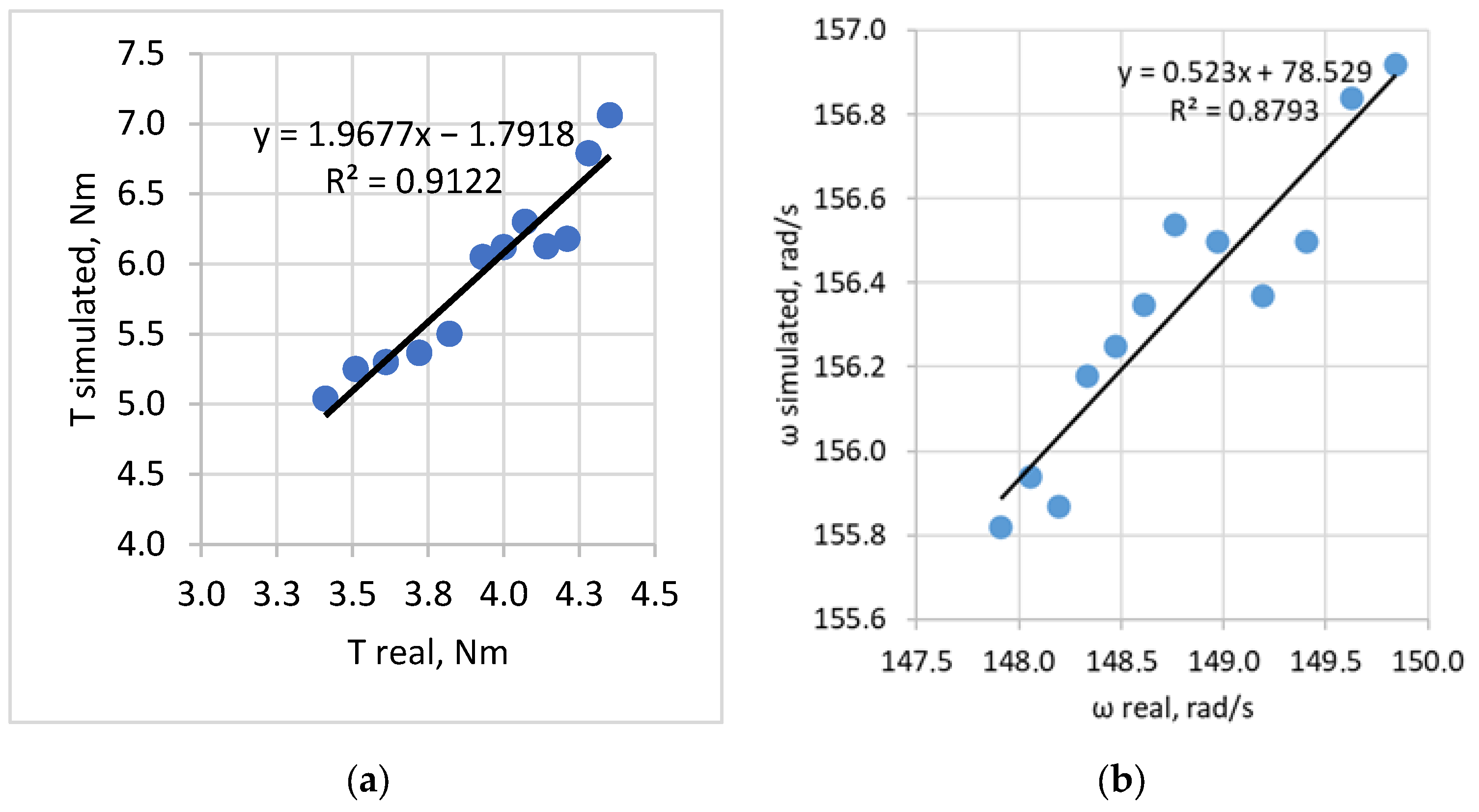
Figure 20 presents comparative plots of torque and angular velocity between the real and simulated electromechanical systems. Although the simulation model predicts higher torque values compared to experimental measurements, the discrepancy remains within acceptable limits for system-level analysis. This confirms that the model is suitable for load assessment, parameter optimization, and the development of control strategies without the need for a complete redesign of its structure.
Table 9 presents comparative results for the errors between the real and simulated electromechanical systems. The sum of squared errors (SSE), root mean square error (RMSE), mean absolute error (MAE), and coefficient of determination (R2) for torque and angular velocity were calculated. The obtained values show a very high degree of correspondence between the real and simulated data with R2 reaching 0.99 for torque and 0.95 for angular velocity. The low values of SSE and RMSE confirm that the differences between the two systems are minimal, and MAE shows a stable and predictable deviation. This demonstrates the good calibration of the model and reliability of the simulation approach in analyzing the dynamics of the electromechanical system.
When comparing the actual measurements and the simulation results, differences are observed in the absolute values of both the torque and the angular velocity. The simulated system predicts higher values compared to the experimental data, which leads to significant deviations reflected in the MAE, SSE, and RMSE metrics. However, the general trend of change remains the same in both cases. Both in the actual measurements and in the simulation, the torque decreases with decreasing mass/load, and the angular velocity increases smoothly. This shows that although the model is shifted in absolute values, it correctly describes the dynamic relationship between the load and the behavior of the electromechanical system, which is important for the validity of the simulation approach.

3.9. Discussion

The results of the experimental measurements and simulations clearly show that the dynamics of the electromechanical system in the automatic bread machine are strongly dependent on the type of flour and the level of hydration of the dough.
Table 10 provides a structured comparison between this paper and related studies, highlighting differences in research focus, modeling approaches, and methodological limitations. The table shows that previous contributions primarily address isolated aspects of the bread-making process such as mechanical design, dough homogeneity, fermentation control, or neural-network-based quality prediction without integrating electromechanical modeling with hydration-dependent viscoelastic load characterization. In contrast, this paper combines physical modeling, PCA, and experimental validation, thereby addressing gaps such as the absence of torque-based load modeling, lack of hydration effects, and limited real-data validation in earlier works.
Modern control approaches such as state-filtered disturbance-rejection control, multilayer neuroadaptive reinforcement learning and actor–critic RL offer high performance for nonlinear systems but require extensive sensing, large datasets, and significant computational resources. These methods are therefore difficult to implement in low-cost consumer appliances, where hardware constraints and the inability to perform safe exploration limit their applicability. In contrast, this paper adopts a lightweight, interpretable modeling approach that can operate with minimal sensing and computation, making it more suitable for embedded monitoring in automatic bread machines. While less sophisticated than advanced RL-based controllers, the proposed method provides transparent relationships between dough properties and mechanical load, enabling practical integration into low-budget systems.
Torque shows the clearest dependence, decreasing by nearly 22–46% as hydration increases from 52% to 63%, which is consistent with the rheological observations of Cappelli et al. [13] and the flour-specific responses described by Niveditha et al. [12]. The slight increase in angular velocity at higher hydration reflects reduced mechanical resistance and aligns with the Maxwell-type viscoelastic behavior incorporated in the model, as also noted by Kuhnert et al. [1].
The energy analysis shows that wholemeal and rye–wheat doughs exhibit a more pronounced reduction in electrical and mechanical energy at higher hydration, supporting the findings of David [15] regarding the higher stiffness of low-hydration doughs. Despite these variations, system efficiency remains stable (η ≈ 0.67), indicating that the electrical subsystem is largely unaffected by load changes, which is similar to the observations of Popov et al. [24].
The MATLAB/Simulink–Simscape simulations demonstrate good agreement with experimental measurements, particularly at medium and high hydration levels. This complements the modeling approaches of Mohammed et al. [22] and Eshkabilov [26]. Deviations at low hydration confirm the known limitations of Simscape in representing highly nonlinear friction and hysteresis effects, as reported by Kittirattanachai et al. [23].
The regression model achieves R2 values between 0.64 and 0.96, reflecting the increasing variability of high-fiber doughs. Compared to neural-network-based approaches [21], the PCA-supported analysis offers higher interpretability and lower computational requirements, making it suitable for low-cost embedded implementations.
The integration of physics-based modeling with high-resolution measurements provides a more accurate representation of the electromechanical–viscoelastic interaction than conventional PI-based designs, which do not account for hydration-dependent load behavior. Higher hydration reduces torque and energy demand within the tested range 52–63%, which demonstrate the potential of the proposed framework for future intelligent control strategies and recipe-aware optimization.

4. Conclusions

This paper demonstrates that integrating system-level electromechanical modeling with high-resolution experimental measurements provides a coherent framework for analyzing the interaction between the motor, transmission, and hydration-dependent viscoelastic load in an automatic bread machine. The results consistently show that higher dough hydration reduces torque and mechanical resistance across all tested flour types, leading to lower energy demand during kneading. These experimentally verified trends align with established rheological findings and confirm the relevance of hydration as a dominant factor influencing the mechanical load.
The combined simulation–experimental approach enables the reproduction of the main dynamic behaviors of the system with MATLAB/Simulink–Simscape models capturing the torque and angular-velocity trends observed in practice. Although the predictive accuracy varies across flour types, the regression analysis provides interpretable relationships between hydration, flour composition, and mechanical load, supporting its use as an analytical rather than a predictive tool.
This paper also shows that low-cost sensing (current, voltage, speed) can be effectively integrated into consumer-grade automatic bread machines, enabling the real-time monitoring of electromechanical variables relevant to process stability and energy use. This highlights a practical pathway for enhancing adaptability and diagnostics in low-budget systems without requiring complex control architectures.
The results obtained can be summarized as follows:
  • Integrated simulation–experimental methodology for analyzing electromechanical systems with viscoelastic loads.
  • Interpretability-focused regression analysis linking hydration and flour type to torque and mechanical power.
  • Validation of Simscape models against extensive experimental measurements.
  • Demonstration of low-cost sensor integration for monitoring electromechanical behavior in bread-making machines.
The limitations of this paper can be summarized as follows:
  • Simplified viscoelastic representation that does not capture all nonlinearities of dough behavior.
  • Single machine platform and a limited hydration range defined by standard bread recipes.
  • Restricted experimental space (three hydration levels, fixed dough mass).
  • No temperature-dependent rheology included in the current model.
Future work should focus on extending the experimental space, incorporating temperature-dependent rheological parameters, refining the viscoelastic model, and developing real-time torque-based control strategies suitable for embedded implementation in commercial bread machines.

Supplementary Materials

The following supporting information can be downloaded at https://www.youtube.com/shorts/sblsd1noMJU (accessed on 24 May 2026); a video with the modified automatic bread machine for the determination of its electromechanical characteristics can be seen.

Author Contributions

Conceptualization, Z.Z. and T.P.; methodology, Z.Z. and M.V.; software, Z.Z.; validation, S.K., T.P. and M.V.; formal analysis, Z.Z. and M.V.; investigation, Z.Z., M.V. and S.K.; resources, Z.Z.; data curation, T.P.; writing—original draft preparation, Z.Z. and M.V.; writing—review and editing, Z.Z. and M.V.; visualization, Z.Z.; supervision, T.P.; project administration, Z.Z.; funding acquisition, Z.Z. All authors have read and agreed to the published version of the manuscript.

Funding

This research was funded by the Bulgarian national program “Development of scientific research and innovation at Trakia University in the service of health and sustainable well-being”—BG-RRP-2.004-006-C02. The APC was funded by the same program.

Institutional Review Board Statement

Not applicable.

Informed Consent Statement

Not applicable.

Data Availability Statement

Additional information can be requested from the corresponding author.

Acknowledgments

We thank Bulgarian national program “Development of scientific research and innovation at Trakia University” for administrative and financial support.

Conflicts of Interest

The authors declare no conflicts of interest.

Abbreviations

The following abbreviations are used in this manuscript:
ACAlternating current
CACalifornia
CFDComputational fluid dynamics
DCDirect current
EMFElectromechanical force
ETAEfficiency
FEMFinite elements modeling
HMIHuman–machine interface
KKTKarush–Kuhn–Tucker
Ltd.Limited company
MAMassachusetts
MAEMean absolute error
MATLABMATrix LABoratory
MSMicrosoft Corporation
PCPrincipal component
PCAPrincipal component analysis
PIDProportional–Integral–Derivative (controller)
RHRelative humidity
RLReinforcement learning
RMSRoot mean squared
RMSERoot mean square error
RPMRevolutions per minute
RWRye–wheat flour
SEStandard error
SPSole proprietorship
SSESum of squared errors
SSRSolid state relay
UKUnited Kingdom
USAUnited States of America
WWhite flour
WWWhole wheat flour

Appendix A

Figure A1 presents an experimental setup for the simulation analysis of an electromechanical control system for an automatic bread machine.
Figure A1. Experimental setup—schematic diagram. 1—single-phase asynchronous electric motor; 2—starting capacitor; 3—belt drive; 4—stirring mechanism; 5—viscoelastic load (bread dough); 6—container in which the dough is kneaded.
Applsci 16 05392 g0a1
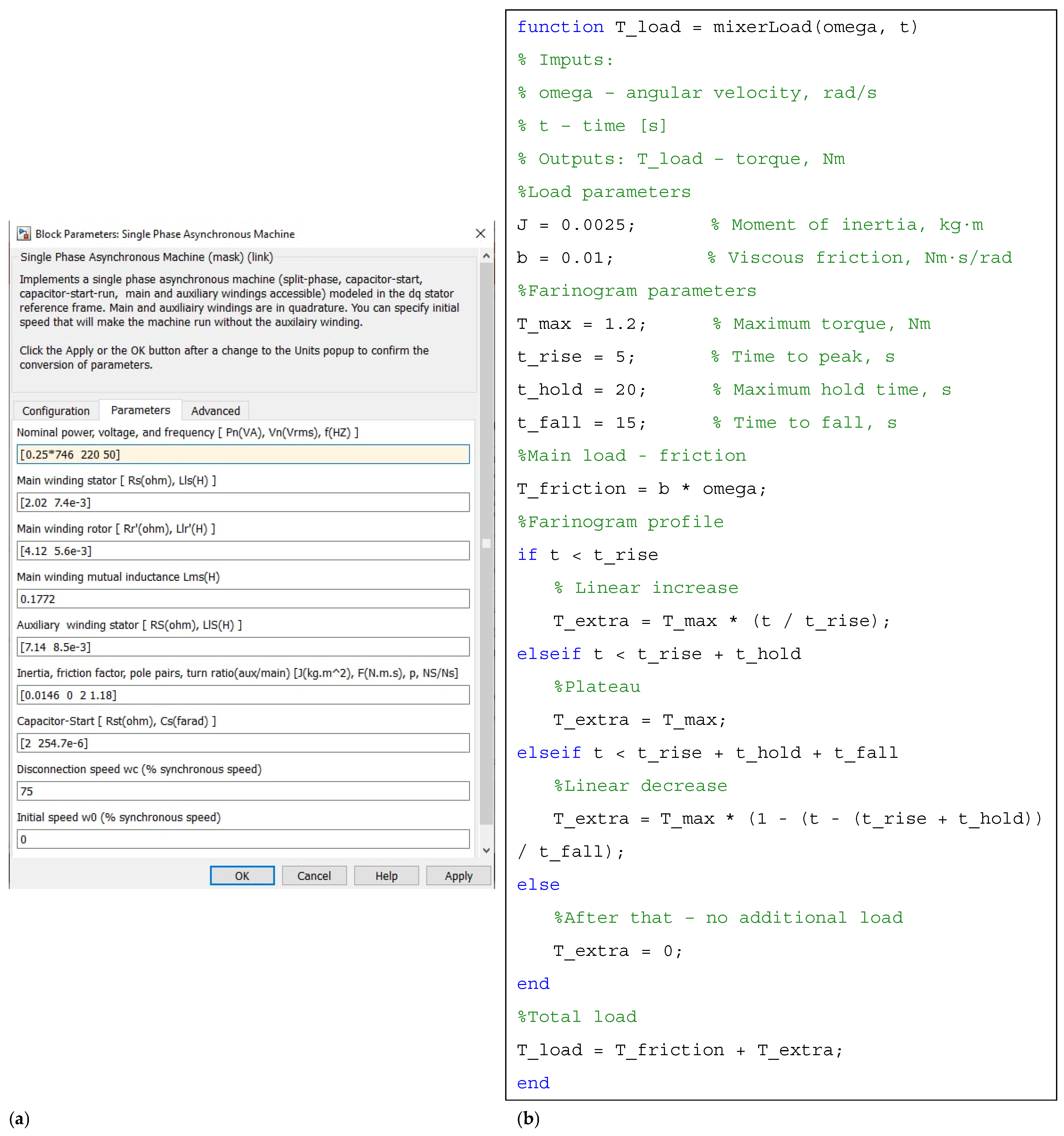
Figure A2 shows the settings of the electric motor and load generation unit. The first part of the figure shows the settings of the single-phase asynchronous motor used in this paper. The motor is bipolar and equipped with a starting capacitor that provides the necessary starting torque. It is configured for a rated apparent power of 105.3 VA, an operating voltage of 220 V, and a frequency of 50 Hz. The model includes the electrical parameters of the main and auxiliary windings, such as their resistances and inductances, as well as the mechanical characteristics of the motor, including its inertia. A capacitor with a capacitance of 4 μF and a resistance of 100 Ω is used during start-up. The auxiliary winding and the capacitor are automatically disconnected once the motor reaches approximately 75% of its synchronous speed, which improves efficiency during steady-state operation. The second part of the figure illustrates the load-generation block that simulates the viscoelastic behavior of the dough during the kneading process. The implemented functional unit reproduces a combined load consisting of viscous friction and a time-dependent farinograph-type torque profile. The viscous component is continuously present and is proportional to the angular velocity of the motor shaft. The farinograph-like component reaches a maximum torque of 1.2 Nm and varies over time to emulate a realistic kneading cycle: it increases linearly during the first 5 s, remains constant for 20 s, and then decreases linearly over the following 15 s before returning to zero. The total load applied to the motor is the sum of these two components, enabling the simulation of a dynamic and realistic viscoelastic load characteristic of dough mixing, where resistance depends both on rotational speed and on the phase of the working process.
Figure A2. Settings of the electric motor and load generation unit: (a) settings of the electric motor; (b) code in the functional block for the load generation unit in the electromechanical system.
Applsci 16 05392 g0a2
Table A1 presents the algorithm for determining the operating point of an AC and DC electric motor. The symbols in the table are as follows: N, rpm—speed of the electric motor; ω, rad/s—angular speed; U, V—supply voltage; I, A—total current of the electric motor, including active and reactive components; Ia, A—current creating torque in the AC motor; cos(φ)—power factor; Iact, A—active component of the current; Ir, A—current in the rotor creating torque; f, Hz—frequency of the supply voltage; p—number of poles of the electric motor; Ns, rpm—synchronous speed of the electric motor; ωs, rad/s—synchronous angular speed of the electric motor; S, a.u.—slip of the electric motor; Pn, W—nominal power; ωn, rad/s—nominal angular velocity; Tn, Nm—nominal torque; Tmax, Nm—maximum torque; Tmot, Nm—torque of the electric motor; Tload, Nm—load torque, linearized load model; I, a.u.—gear ratio (ratio) of the belt drive; ωmix, rad/s—angular speed after the belt drive; Tmix, Nm—torque after the belt drive; ωwp, rad/s—angular speed at the operating point; Twp, Nm—torque at the operating point; a and b are coefficients of the load characteristic equation.
Table A1. Algorithm for determining the operating point of an AC electric motor.
StageNameEquationNumber
1Conversion of revolutions into angular velocity ω = 2 π N 60 (A1)
2Active current (active component) I a c t = I c o s ( φ ) (A2)
3Rotor current I r = s I a c t (A3)
4No load speed (synchronous speed) n s = 120 f p (A4)
5No load angular velocity (synchronous angular velocity) ω 0 = 2 π N s 60 (A5)
6Nominal angular velocity ω n = 2 π N n 60 (A6)
7Nominal torque T n = P n ω n (A7)
8Stall torque (maximum torque) T m a x 2.5 T n (A8)
9Mechanical characteristic T = T m a x ω s ω ω s ω m i n (A9)
10Slip S = N s N N s (A10)
11Load characteristic T l o a d = a ω + b (A11)
12Operating point T ω w p = T l o a d ω w p (A12)
13After belt drive ω m i x = ω i ;   T m i x = T i (A13)
14Mechanical characteristic after gearing T m o t ,   m i x = T m a x i 1 ω ω s i (A14)
15Operating point after gearing T m o t ,       m i x = T l o a d ,       m i x (A15)
Table A2 presents the hardware used to build a device for determining the characteristics of an electromechanical system of an automatic bread machine. The Mega 2560 single-board microcomputer is used to execute programs for controlling electronic components, while the Nextion Intelligent 4.3” NX4827P043-011 touch display visualizes data and accepts commands by touch. The Vemark VGX-4825DA TRIAC switch is used for contactless switching of electrical circuits, and the HM-550 (MAX6675) digital amplifier converts an analog signal from a thermocouple into digital temperature data. The power supply unit converts the mains voltage from 220V AC to 5V DC for powering electronic devices. Capacitors 470 µF, 16V DC MKP10 and Vemark 4 µF ±5% stabilize the voltage and filter electrical signals. The CBM-6511 automatic bread machine was used as the basis for creating the experimental model of an electromechanical system. The ACS712 5A current sensor measures the electric current in the electric motor circuit, and the frequency sensor F249 monitors its rotation speed.
Table A2. Technical specification of the selected hardware.
ModelType of the DeviceManufacturerCity, Country
Mega 2560Single-board microcomputerSunfounder Inc., Shenzhen, Chinahttps://www.sunfounder.com (accessed on 10 February 2025)
Nextion Intelligent 4.3” NX4827P043-011Touch-sensitive displayITEAD Intelligent Systems Co., Ltd.Shenzhen, China
Vemark VGX-4825DATRIAC switch (SSR)Vikiwat Ltd.Plovdiv, Bulgaria
HM-550, based on integrated circuit Max6675Digital thermocouple amplifierChipskey Technology Co., Ltd.Shenzhen, China
220V AC to 5V DC, 2APower supply unitPenghan New energy Co., Ltd.Wenzhou, China
470 µF, 16V DC MKP10CapacitorWIMA GmbH & Co. KGMannheim, Germany
Vemark 4 µF ± 5%CapacitorVikiwat Ltd.Plovdiv, Bulgaria
CBM-6511, 600 WAutomatic bread machineCrownShanghai, China
ACS712 5ACurrent sensorAllegro Micro Systems, Inc.Worcester, MA, USA
F249Speed sensorDAOKIShenzhen, China
To create a voltage sensor, a basic electronic circuit presented in (https://www.instructables.com/AC-Voltmeter-Using-Arduino (accessed on 25 May 2025)) was used.
The circuit of the voltage sensor is presented in Figure A2. The voltage of 200 V AC is reduced to 6 V AC by a transformer. A voltage divider with 1 kΩ resistors is used. The 1N4007 rectifier diode cuts off the lower half-wave of the sinusoidal signal. The 470 µF capacitor smooths the resulting voltage signal. The Zener diode limits the voltage to 5 V DC. The output from the sensor is connected to an analog input of a single-board microcomputer.
Figure A3. Voltage sensor—electrical diagram.
Applsci 16 05392 g0a3
The analog input of the single board computer is 10 bit. For this reason, the 0–5 V DC signal is represented as 0–1023 bit. It is necessary to calculate the V/bit ratio, according to the following formula:
U m a x = b 311 1023 , V
where b is the value (0–1023) obtained from the ADC of the single-board microcomputer.
The conversion of the signal from the sensor is performed by calculating the effective value of the input voltage (Urms). It is calculated from the peak value of the voltage (Umax) according to the following formula:
U r m s = U m a x 2 , V
Table A3 shows in tabular form the algorithm of the software support of an electromechanical system control system. The algorithm implements the control and monitoring of an electromechanical system using a microcontroller that measures and processes physical quantities such as temperature, voltage, current, and revolutions (RPM); then, it calculates power, torque, and derivative value tmix; and the results are visualized through a connected Nextion display. In the initial phase, the initialization of pins and serial connections is performed. In the main cycle (loop), the sensors provide data on temperature, voltage, and current, and the calculations are used to determine the current parameters of the system. The data are sent to the display in both text and graphical form. The algorithm monitors commands from the user (such as “start motor” or “stop”), processes them, and controls the motor and PID control to maintain a set temperature.
Table A3. Algorithm of software for an electromechanical system control system.
FunctionDescription
Input DataI, A; U, V; N, rpm; Display Button Status
1Initialization (setup)Setting pins, starting serial communication with: Serial, Serial2 (Nextion), Serial3
2Determine RPMWith the help of calculateRPM(), by input from pin 7
3Measure temperatureFrom MAX6675 thermocouple via .readCelsius()
4Measure voltagereadVoltage()—via analog input A0
5Measure currentreadCurrent()—via analog pin A5 with conversion calculations
6Calculate power (W)power = voltage × current
7Calculate torquecalculateTorque()—uses RPM and power
8Calculate tmixtmix = torque × 0.105
9Send to displaySends all measured values to the Nextion display via sendToNextion()
10Send commands to graphVisualization commands (“add 5,2,” and “add 5,0,”)
11Process input commandsAccepting commands from Nextion (via Serial2) when 0xFF is received 3 times
12Call processCommandAnalysis of display commands (startmotor, stopmotor, start, stop)
Output dataP, W; T, Nm; Tmix, Nm; text and graphic visualization on the display
The input data entry and the calculation of the output variables are implemented in the form of subroutines. Table A4 lists these subroutines. The subroutines in the algorithm ensure the modular and efficient operation of the system by performing specific control, measurement, calculation and visualization tasks. They process input commands (processCommand, continuous), control the operating mode of the electric motor (mix), implement communication with the display (sendToNextion), and perform measurements from voltage, current and speed sensors (readVoltage, readCurrent, calculateRPM). Calculations for torque and (Tmix) are performed by (calculateTorque), and PID temperature control is implemented by the function (pid), which controls the heater via a PWM signal.
Table A4. Subroutines in the software of an electromechanical control system.
FunctionDescription
processCommand()Registers commands from the display: start/stop of the electric motor (with or without timer)
mix(uint32_t d1)Interval start of the electric motor for a set time (in minutes). Controls icons on the Nextion display
continuous(cmd)Starts the PID controller and starts the electric motor continuously until it receives a stop command
sendToNextion()Sends values to the display in the required format with terminators 0xFF
readVoltage()Reads an analog signal and calculates voltage (calibrated with coefficients)
readCurrent()Converts analog input to the effective value of the current using the appropriate formula
calculateRPM()Reads pulsations from the speed sensor and converts them to revolutions per minute (every 4 s)
calculateTorque()Calculates the electric motor torque T, Nm and the agitator torque Tmix, Nm
pid(Setpoint)PID temperature controller: regulates the PWM of the heater (HEATER_PIN) relative to a set value
Using the Nextion Editor programming system, a graphical user interface (HMI) of software for controlling the electromechanical system of an automatic bread machine has been developed. This HMI consists of four screens (Figure A4).
Figure A4. Graphical user interface of software for controlling the electromechanical system of an automatic bread machine: (a) main screen; (b) screen “mixing”; (c) data acquisition screen; (d) help screen.
Applsci 16 05392 g0a4
From the main screen, the necessary function for controlling the electromechanical system is selected. The temperature in the kneading chamber is visualized on the “Mixing” screen as well as the switching on and off of the electric motor. It operates cyclically, its operation being visualized by means of round indicators “On” and “Off”, respectively. The electric motor is started and stopped by the “Start” and “Stop” buttons.
On the data recording screen, the change in the electric motor torque is observed in graphic form. The values of the main characteristics of the electromechanical system are presented, which are measured in real time. The electric motor is started and stopped by the “Start” and “Stop” buttons. The “Help information” screen presents guidelines (instructions) for working with the electromechanical control system.
When operating the electromechanical system of an automatic bread machine, it is necessary to maintain the water temperature at around 30 °C, as this provides appropriate conditions for dough preparation. For this purpose, a PID controller has been implemented as a subroutine in the control software.
Figure A5 shows the method used for L-a approximation of the object. The temperature object is assumed to be self-regulating, and for this reason, the Ziegler–Nichols L-a approximation method has been used.
Figure A5. Determining the PID controller settings by the transient characteristic of the controlled object.
Applsci 16 05392 g0a5
The PID controller settings are implemented using the following formulas:
k p = 1.2 a
T i = 2 L
k i = 1 T i
k d = L 2
α = T s L a + T s
where L and a are the time and temperature, which are determined with the L-a approximation; Kp is the proportional coefficient of the controller; Ti is the integration time; Ki is the integration coefficient; Kd is the differentiation coefficient; α is the filter coefficient of the differential part of the controller; and Ts is the time interval for each temperature measurement.
Figure A6 shows in graphic form how the parameters for setting the PID temperature controller are determined.
After smoothing the transient characteristic, a tangent is drawn to it. At the intersection points of the tangent to the horizontal and vertical axes, an L-a approximation is made.
Figure A6. Determining the parameters for tuning a PID temperature controller using L-a approximation.
Applsci 16 05392 g0a6
The parameters of the PID temperature controller are determined. Table A5 shows the calculated settings of the controller and those obtained after fine tuning. Kp is increased by 1.2 times, Ki is increased by about 1.6 times, Kd is reduced by 1.4 times, and α is reduced by 0.3. From this, it follows that the calculated and fine-tuned parameters of the controller have a minimal difference.
Table A5. PID controller settings.
ParameterCalculated ValueSet Value
a0.225-
L71-
Kp5.336.5
Ti142-
Ki0.0070.011
Kd35.525
α0.240.21
Figure A7 shows the result of the operation of the PID temperature controller. The peaks in the measured values are due to the fact that the object is not sufficiently polished by the environment, and interference occurs. The averaged characteristics show that the controller can maintain the set temperature of 30 °C.
Figure A7. Transient process of a closed temperature control system.
Applsci 16 05392 g0a7
Figure A8 shows dough prepared in an automatic bread machine. The dough from type 500 flour shows classic gluten network behavior. At low hydration (52%), the structure is stiffer and has high deformation strength, which correlates with a higher measured torque. Medium hydration (58%) leads to a balance between elasticity and plasticity, while at 63%, the dough becomes softer and viscous, which reduces the resistance to mixing and, accordingly, the torque.
Wholemeal dough made from 1850 flour has a higher water-holding capacity due to the presence of fiber and bran. This results in a weaker and more tearable gluten network, a higher initial density and greater mechanical resistance at low hydration. At 52%, the dough is the stiffest and generates the highest torque of the three flour types, while at 63% it becomes more plastic, leading to a distinct reduction in the load on the electric motor. Rye–wheat dough has a dominant viscous behavior due to the limited formation of the gluten network. It absorbs more water but remains sticky and with lower elasticity. This results in moderate torque values at low hydration and a smoother reduction in load as the water content increases. The visually stickier and denser structure at 52% corresponds to higher mechanical resistance, while the softer consistency at 63% correlates with distinctly lower torques.
Figure A8. Dough prepared in an automatic bread machine with an electromechanical system driven by a single-phase asynchronous electric motor—general view: (a) water 52%; (b) water 58%; (c) water 63%; W—dough made from white flour; WW—dough made from whole wheat flour; RW—dough made from rye–wheat flour.


Applsci 16 05392 g0a8

References

  1. Kuhnert, W.M.; Cammarano, A.; Silveira, M.; Gonçalves, P.J.P. Synthesis of Viscoelastic Behavior Through Electromechanical Coupling. J. Vib. Eng. Technol. 2021, 9, 367–379. [Google Scholar] [CrossRef]
  2. Liu, S.; Yu, H.; Ding, N.; He, X.; Liu, H.; Zhang, J. Exploring Modeling Techniques for Soft Arms: A Survey on Numerical, Analytical, and Data-Driven Approaches. Biomimetics 2025, 10, 71. [Google Scholar] [CrossRef]
  3. Fu, Q.; Nicholson, G.L.; Easton, J.M. Understanding Data Quality in a Data-Driven Industry Context: Insights from the Fundamentals. J. Ind. Inf. Integr. 2024, 42, 100729. [Google Scholar] [CrossRef]
  4. Olugbade, T.O.; Ojo, O.T. Development and performance evaluation of an improved electric baking oven. Leonardo Electron. J. Pract. Technol. 2018, 33, 189–206. [Google Scholar]
  5. Murugesan, M.; Pandurangan, P.; Murugesan, A.; Senthilkumar, H.; Hegde, K.K.; Thangaraj, S.; Moovendhan, M. Artificial Intelligence in Bread Making: Applications in Quality Control, Formulation and Sensory Prediction. Food Chem. X 2026, 34, 103654. [Google Scholar] [CrossRef]
  6. Zhao, S.; Jiao, T.; Adade, S.Y.-S.S.; Wang, Z.; Ouyang, Q.; Chen, Q. Digital Twin for Predicting and Controlling Food Fermentation: A Case Study of Kombucha Fermentation. J. Food Eng. 2025, 393, 112467. [Google Scholar] [CrossRef]
  7. Smith, L.P.; Ng, S.W.; Popkin, B.M. Trends in US home food preparation and consumption: Analysis of national nutrition surveys and time use studies from 1965–1966 to 2007–2008. Nutr. J. 2013, 12, 45. [Google Scholar] [CrossRef]
  8. Horská, E.; Urgeová, J.; Prokeinová, R. Consumers’ food choice and quality perception: Comparative analysis of selected Central European countries. Agric. Econ. 2011, 57, 493–499. [Google Scholar] [CrossRef]
  9. Mashal, I.; Shuhaiber, A.; Al-Khatib, A.W. User acceptance and adoption of smart homes: A decade long systematic literature review. Int. J. Data Netw. Sci. 2023, 7, 533–552. [Google Scholar] [CrossRef]
  10. Fatoki, O. Factors influencing the purchase of energy-efficient appliances by young consumers in South Africa. Found. Manag. 2020, 12, 151–166. [Google Scholar] [CrossRef]
  11. Raffak, A.; Chafai, Y.; Toure, I.; Hamouda, A.; Ismaili Alaoui, M.; Ouazzani Touhami, A.; Mounir, M. Real-Time Monitoring Device “Panigraph” for Bread Fermentation with an Arduino-Based Data Acquisition and Management System. Mor. J. Agri. Sci. 2023, 4, 185–193. [Google Scholar]
  12. Niveditha, A.; Chidanand, D.V. Assessment of Dough Rheological Characteristics with Mixing Time. Indian J. Pure Appl. Biosci. 2019, 7, 269–276. [Google Scholar] [CrossRef]
  13. Cappelli, A.; Bettaccini, L.; Cini, E. The Kneading Process: A Systematic Review of the Effects on Dough Rheology and Resulting Bread Characteristics, Including Improvement Strategies. Trends Food Sci. Technol. 2020, 104, 91–101. [Google Scholar] [CrossRef]
  14. Ntalios, E.; Raphaelides, S.; Marinopoulou, A. An Investigation of Changes in the Rheological Properties of Toast Pan Bread Dough During the Various Processing Steps of Kneading in an Industrial Bakery. Gastronomy 2024, 2, 57–72. [Google Scholar] [CrossRef]
  15. David, I. The Enzyme Activity of Hemicellulase Used on Dough Obtained from Wheat Flour. Actual Tasks Agric. Eng. 2014, 42, 353–363. [Google Scholar]
  16. Voicu, G.; Constantin, G.; Ipate, G.; Tudor, P. Farinographic Parameter Variation of Doughs from Wheat Flour with Amount of Water Added. In Proceedings of the International Scientific Conference Engineering for Rural Development, Jelgava, Latvia, 24–26 May 2017; pp. 976–981. [Google Scholar]
  17. Okafor, B.E. Design of Power Driven Dough Mixing Machine. Int. J. Eng. Technol. 2015, 5, 76–79. [Google Scholar]
  18. Orelaja, O.A.; Alabi, A.A.; Tiamiyu, O.A.; Adeogun, O. Design and Fabrication of an Improved Industrial Impeller Dough Mixer. Int. J. Eng. Sci. 2020, 9, 36–43. Available online: https://www.theijes.com/papers/vol9-issue11/D0911013643.pdf (accessed on 24 May 2026).
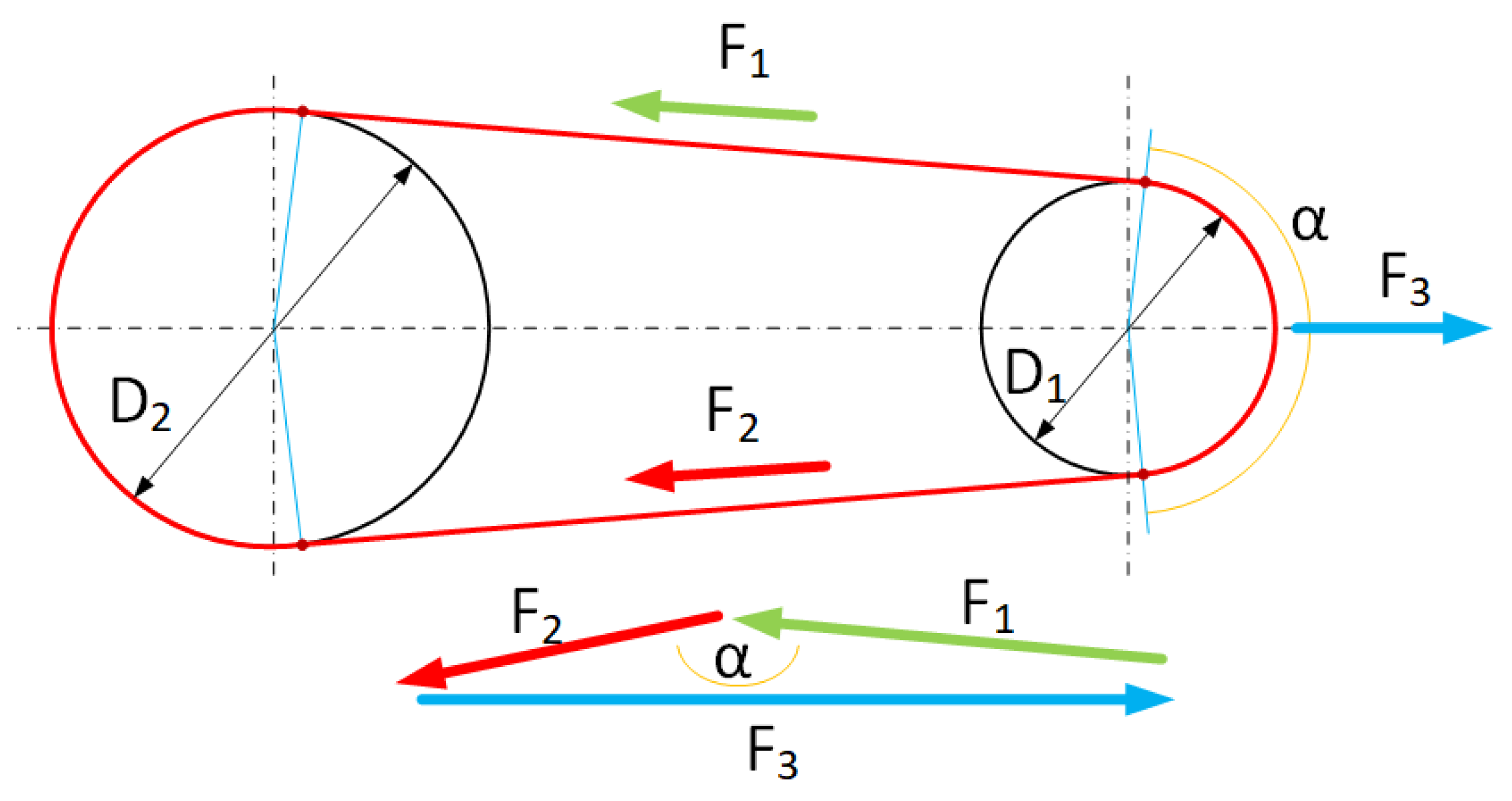
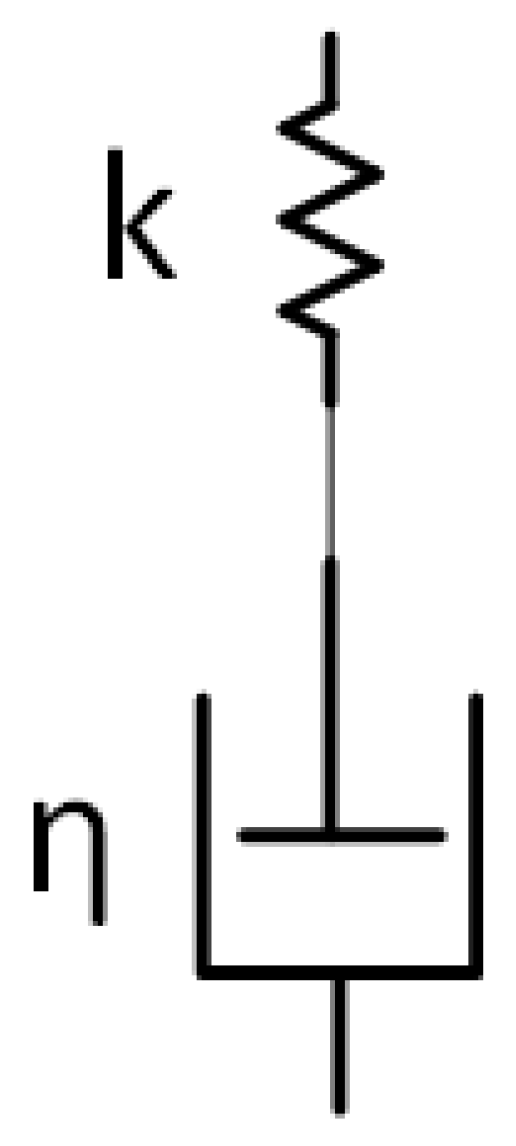
  19. Abdul Fatah, I.Y.; Ramli, N.A.B.; Rohimi, R. Conceptual Design and Simulation Analysis of Dough Mixer-Maker Machine. Malays. J. Appl. Sci. 2022, 7, 93–102. [Google Scholar] [CrossRef]
  20. Hsu, E.J. Design of a Measurement Device for Bread Dough Proofing. Master’s Thesis, Massachusetts Institute of Technology, Cambridge, MA, USA, 2020. [Google Scholar]
  21. Lee, J.; Kim, Y.; Kim, S. The Study of an Adaptive Bread Maker Using Machine Learning. Foods 2023, 12, 4160. [Google Scholar] [CrossRef]
  22. Mohammed, F.M.; Mohammed, J.A.-K.; Faisl, H. Modeling and simulation of an electromechanical brake system. IOP Conf. Ser. Mater. Sci. Eng. 2021, 1105, 012051. [Google Scholar] [CrossRef]
  23. Kittirattanachai, A.; Watechagit, S. Simulated braking performance comparison of an electric drum brake and a hydraulic drum brake systems. IOP Conf. Ser. Mater. Sci. Eng. 2020, 886, 012031. [Google Scholar] [CrossRef]
  24. Popov, M.; Negodin, A. Simulation on elevator emergency brake. IOP Conf. Ser. Mater. Sci. Eng. 2021, 1118, 012029. [Google Scholar] [CrossRef]
  25. Aires de Freitas, F.B.; Pereira, L.R.; Dias da Silva Cabral, L.; Cavallini, A.A.; Steffen, V. Numerical modeling and experimental analysis of structural integrity monitoring of mechanical systems based on electromechanical impedance. J. Nondestruct. Eval. 2026, 45, 41. [Google Scholar] [CrossRef]
  26. Eshkabilov, S.L. Practical MATLAB Modeling with Simulink: Programming and Simulating Ordinary and Partial Differential Equations, 1st ed.; Apress: New York, NY, USA, 2020. [Google Scholar] [CrossRef]
  27. Cunha, A.; Pereira, M.; Avanço, R.; Tusset, A.M.; Balthazar, J.M. ElectroM: ElectroMechanical dynamic code. Softw. Impacts 2023, 17, 100533. [Google Scholar] [CrossRef]
  28. Dochev, M. Simplified Method of Defining the Torque, the Shaft Load Moment and the Moment of Inertia for Power Tools. In Proceedings of the ELMA 2008, TU-Sofia, Bulgaria, 16–18 September 2008; pp. 323–324. [Google Scholar]
  29. Dochev, M.; Bojilov, G. Diagnostic Computing Model of a Single-Phase Commutator Motor for Power Tools. In Proceedings of the International Conference on Electrical Machines, Drives and Power Systems (ELMA ’99), Varna, Bulgaria, 22–25 September 1999; pp. 106–109. [Google Scholar]
  30. Nikolova, I.; Dahterova, D.; Ivanov, V.; Lemu, H. Comparative Study of PROMETHEE II and RAZOR Methods for Multi-Criteria Optimization of Electromechanical Modules. Teh. Vjesn. 2018, 25, 1330–1338. [Google Scholar] [CrossRef]
  31. Yordanov, P.; Spirov, D.; Dochev, M. Power Tools Performance Characteristics at Dynamic and Steady-State Regimes. In Proceedings of the 9th International Conference “Research and Development in Mechanical Industry” (RaDMI 2009), Vrnjačka Banja, Serbia, 16–19 September 2009; pp. 1258–1263. [Google Scholar]
  32. Tec-Science. Power Transmission of a Belt Drive. 2025. Available online: https://www.tec-science.com/mechanical-power-transmission/belt-drive/power-transmission-of-a-belt-drive (accessed on 16 June 2025).
  33. Roylance, D. Engineering Viscoelasticity; Report; Massachusetts Institute of Technology: Cambridge, MA, USA, 2001; pp. 8–11. Available online: https://web.mit.edu/course/3/3.11/www/modules/visco.pdf (accessed on 30 May 2025).
  34. Weinerowska-Bords, K. Viscoelastic Model of Waterhammer in Single Pipeline—Problems and Questions. Arch. Hydro-Eng. Environ. Mech. 2006, 53, 331–351. [Google Scholar]
  35. Bonfanti, A.; Kaplan, J.L.; Charras, G.; Kabla, A. Fractional Viscoelastic Models for Power-Law Materials. Soft Matter 2020, 16, 6002–6020. [Google Scholar] [CrossRef]
  36. Launay, B. A Simplified Nonlinear Model for Describing the Viscoelastic Properties of Wheat Flour Doughs at High Shear Strain. Cereal Chem. 1990, 67, 25–31. [Google Scholar]
  37. Altuna, L.; Romano, R.C.O.; Pileggi, R.G.; Ribotta, P.D.; Tadini, C.C. Torque Measurement in Real Time During Mixing and Kneading of Bread Dough with High Content of Resistant Maize Starch and Enzymes. Int. J. Food Eng. 2016, 12, 719–728. [Google Scholar] [CrossRef]
  38. Fanari, F.; Naue, I.F.C.; Desogus, F.; Grosso, M.; Wilhelm, M. Durum Wheat Dough Torque Measurements: Characterization and Study of the Mixing Process Parameters as a Function of Water and Salt Amounts. Chem. Eng. Trans. 2021, 87, 205–210. [Google Scholar] [CrossRef]
  39. Robnik-Šikonja, M.; Kononenko, I. Theoretical and Empirical Analysis of ReliefF and RReliefF. Mach. Learn. 2003, 53, 23–69. [Google Scholar] [CrossRef]
  40. Stock, A.; Subramaniam, A. Iterative spatial leave-one-out cross-validation and gap-filling based data augmentation for supervised learning applications in marine remote sensing. GIScience Remote Sens. 2022, 59, 1281–1300. [Google Scholar] [CrossRef]
  41. Teodorescu, V.; Obreja Brașoveanu, L. Assessing the Validity of k-Fold Cross-Validation for Model Selection: Evidence from Bankruptcy Prediction Using Random Forest and XGBoost. Computation 2025, 13, 127. [Google Scholar] [CrossRef]
  42. Yadav, S.; Shukla, S. Analysis of k-Fold Cross-Validation over Hold-Out Validation on Colossal Datasets for Quality Classification. In Proceedings of the 2016 IEEE 6th International Conference on Advanced Computing (IACC), Bhimavaram, India, 27–28 February 2016; pp. 78–83. [Google Scholar]
  43. Gewers, F.L.; Ferreira, G.R.; Arruda, H.F.D.; Silva, F.N.; Comin, C.H.; Amancio, D.R.; Costa, L.D.F. Principal Component Analysis: A Natural Approach to Data Exploration. ACM Comput. Surv. 2021, 54, 70. [Google Scholar] [CrossRef]
  44. Emmert-Streib, F.; Dehmer, M. Evaluation of Regression Models: Model Assessment, Model Selection and Generalization Error. Mach. Learn. Knowl. Extr. 2019, 1, 521–551. [Google Scholar] [CrossRef]
  45. Konuhova, M. Induction Motor Dynamics Regimes: A Comprehensive Study of Mathematical Models and Validation. Appl. Sci. 2025, 15, 1527. [Google Scholar] [CrossRef]
  46. Liu, Y.; Zhang, L.; Li, P.; Xu, Y. Active Disturbance Rejection for Linear Induction Motors: A High-Order Sliding-Mode-Observer-Based Twisting Controller. Actuators 2025, 14, 200. [Google Scholar] [CrossRef]
  47. Trivedi, P.; Hemachandra, N. Multi-Agent Natural Actor-Critic Reinforcement Learning Algorithms. Dyn. Games Appl. 2023, 13, 25–55. [Google Scholar] [CrossRef]
  48. Pycia, K.; Juszczak, L. Rheological Characteristics of Wheat Dough Containing Powdered Hazelnuts or Walnuts Oil Cakes. Foods 2024, 13, 140. [Google Scholar] [CrossRef]
  49. Hamani, K.; Kuchar, M.; Kubatko, M.; Kirschner, S. Advancements in Induction Motor Fault Diagnosis and Condition Monitoring: A Comprehensive Review. Sensors 2025, 25, 5942. [Google Scholar] [CrossRef]
Figure 1. Block diagram of the proposed electric drive measurement and control system.
Applsci 16 05392 g001
Figure 2. Forces acting in a belt drive.
Applsci 16 05392 g002
Figure 3. Maxwell’s model.
Applsci 16 05392 g003
Figure 4. Workflow of the computational procedure.
Applsci 16 05392 g004
Figure 5. Simulation diagram of an electromechanical system with a viscoelastic load.
Applsci 16 05392 g005
Figure 6. Simulation circuit of a voltage sensor.
Applsci 16 05392 g006
Figure 7. Averaged change in electrical characteristics of the electric motor at different bread dough masses. (a) Electrical characteristics; (b) motor and load torque.
Applsci 16 05392 g007
Figure 8. Averaged characteristics of the simulation results when changing the amount of water in dough. (a) Electrical characteristics; (b) motor and load torque.
Applsci 16 05392 g008
Figure 9. Model of the type T = f(M, W)–general form.
Applsci 16 05392 g009
Figure 10. Control system for electromechanical system of an automatic bread machine—electrical diagram.
Applsci 16 05392 g010
Figure 11. Electromechanical dough preparation system—general view. 1—personal computer for recording and subsequent analysis of data; 2—vessel with a stirring element; 3—voltage sensor; 4—single-board microcomputer; 5—electric motor with a mounted measuring disk with holes; 6—speed sensor; 7—heater; 8—thermocouple; 9—thermocouple sensor-amplifier; 10—current sensor; 11—analog voltmeter; 12—analog ammeter; 13—display; 14—SSR switch for the heater; 15—TRIAC switch for the electric motor; 16—power supply unit; 17—belt drive located under the dough vessel.
Applsci 16 05392 g011
Figure 12. Averaged characteristics of the electric motor when kneading dough from type 500 flour: (a) voltage; (b) current; (c) motor RPM.
Applsci 16 05392 g012
Figure 13. Averaged characteristics T = f(ω) for a dough load of type 500 flour: (a) water 52%; (b) water 58%; (c) water 63%.
Applsci 16 05392 g013
Figure 14. Averaged characteristics of the electric motor when kneading dough from flour type 1850: (a) voltage; (b) current; (c) motor RPM.
Applsci 16 05392 g014
Figure 15. Averaged characteristics T = f(ω) for a load of wholemeal flour dough type 1850: (a) water 52%; (b) water 58%; (c) water 63%.
Applsci 16 05392 g015
Figure 16. Averaged characteristics of the electric motor when kneading dough from rye–wheat flour: (a) voltage; (b) current; (c) motor RPM.
Applsci 16 05392 g016
Figure 17. Averaged characteristics T = f(ω) for a load of rye–wheat flour dough: (a) water 52%; (b) water 58%; (c) water 63%.
Applsci 16 05392 g017
Figure 18. Results of selection of informative features. U—voltage; I—current; N—revolutions (RPM); E—induced electromechanical force; ω—angular velocity of the electric motor; ω_mix—angular velocity of the mixer; Pe—electric power of the electric motor; T—torque of the electric motor; T_mix—torque of the mixer; Pm—mechanical power of the mixer; S—full power of the electric motor; ETA—efficiency; cos(φ)—power factor.
Applsci 16 05392 g018
Figure 19. Results of principal component analysis. W—white flour; WW—whole wheat flour; RW—rye–wheat flour; U—voltage; I—current; Pe—electric power of the electric motor; T_mix—torque of the mixer; Pm—mechanical power of the mixer; S—full power of the electric motor; ETA—efficiency; cos(phi)—power factor.
Applsci 16 05392 g019
Figure 20. Comparative graphs between real and simulated electromechanical system: (a) torque; (b) angular speed.
Applsci 16 05392 g020
Table 1. Data for an electric motor of an automatic bread machine.
CharacteristicDesignation and Measurement UnitValue
AC supply voltageU, V220
Rated powerPn, W100
Rated AC currentI, A0.5
Inductance of windingsL, H0.158
Resistance of windingsR, Ω126.2
Number of polesp, number4 (2 pole pairs)
Synchronous speedNs, rpm1500
Angular speedωn, rad/s157
Rated speedNn, rpm ≈1400–1470
Rated torqueTn, Nm0.637
cosφa.u.0.95
SlipS, a.u.≈0.07–0.02
Table 2. Initial data for the mechanical transmission of an automatic bread machine.
CharacteristicDesignation and Measurement UnitValue
Drive pulley diameterD, m0.13
Driven pulley diameterDmix, m0.011
Belt drive efficiencya.u.0.95
Agitator radiusrmix, m0.06
Table 3. Description of viscoelastic load of the electromechanical system.
Average Dough Weight, gMaximum Load Torque Tmix, NmDescription of the LoadBread Mass, gBread Size Description
5805.57Light load500Small for 1–2 people
8807.01Standard load750Standard/family
10507.49Heavy load1000Large/for 3–4 people
Table 4. Viscoelastic load parameters (dough).
Water, %Viscous Friction
b, Nm·s/rad
Maximum Load Torque
T_mix, Nm
Description of the Dough
500.017.06Firmer
600.0086.05Standard
700.0055.04Softer
Table 5. Operating points of an electromechanical system with an alternating current electric motor for different types of flour and hydration levels.
Flour Type Parameterω, rad/sT, Nmωmix, rad/sTmix, Nm
Water, %
White 52147.91 ± 13.960.51 ± 0.117.4 ± 1.474.35 ± 0.49
58148.76 ± 28.830.46 ± 0.0917.5 ± 0.023.93 ± 0.65
63149.84 ± 6.540.4 ± 0.0517.63 ± 0.633.41 ± 0.09
Whole wheat52147.91 ± 2.190.51 ± 0.0517.4 ± 2.214.37 ± 0.1
58149.04 ± 12.50.44 ± 0.0717.53 ± 3.453.74 ± 0.09
63151.9 ± 4.140.28 ± 0.0317.87 ± 0.322.36 ± 0.16
Rye–wheat 52149.06 ± 4.270.45 ± 0.0517.54 ± 2.563.83 ± 0.4
58149.86 ± 6.870.39 ± 0.0317.63 ± 0.93.33 ± 0.39
63151.34 ± 24.290.3 ± 0.0317.8 ± 3.112.54 ± 0.22
Table 6. Energy balance, losses and efficiency of the electromechanical system.
CharacteristicWater, %We, JWm, JWloss, JEfficiencycos(φ)
Flour Type
White 52117,849.72 ± 11,777.3879,548.56 ± 10,380.7738,301.16 ± 1710.780.67 ± 0.130.85 ± 0.06
58117,621.54 ± 21,406.9479,394.54 ± 1980.0338,227 ± 5303.80.67 ± 0.110.85 ± 0.16
63117,293.93 ± 3520.0579,173.4 ± 15,479.7838,120.53 ± 423.270.67 ± 0.050.85 ± 0.07
Whole wheat52118,657.31 ± 16,855.2780,093.68 ± 7639.8538,563.62 ± 3229.270.67 ± 0.110.85 ± 0.03
58116,344.9 ± 4707.3378,532.81 ± 13,576.2937,812.09 ± 452.030.67 ± 0.050.85 ± 0.08
63114,222.57 ± 4629.3877,100.24 ± 2830.7937,122.34 ± 4729.520.67 ± 0.110.85 ± 0.16
Rye–wheat 52118,944.88 ± 18,791.0780,287.79 ± 4251.638,657.09 ± 3813.530.67 ± 0.070.85 ± 0.11
58115,438.1 ± 4076.6377,920.72 ± 9647.5537,517.38 ± 437.660.67 ± 0.040.85 ± 0.1
63111,220.97 ± 21,062.5375,074.15 ± 6034.1536,146.82 ± 1417.550.67 ± 0.070.85 ± 0.07
We—electrical energy of the electric motor; Wm—mechanical energy of the electric motor; Wloss—energy losses in the electric motor; cos(φ)—power factor.
Table 7. Results from cross-validation of the selected features.
CriteriaRMSEMAESSER2
Method
K-Fold (10)0.480.396.720.87
Hold-Out (70/30)0.520.418.110.85
Leave-One-Out0.460.386.630.88
Table 8. Comparative analysis of a real (experimental) and simulated electromechanical system.
Researched SystemReal System (Experiment)Simulated System (Simulink/Simscape)
Characteristic
Supply voltage (U)220 V AC220 V AC (configured in the model)
Motor rated power100 W105.3 VA
Load torque (Tmix)3.33–4.37 Nm (for 300 g flour at 52–63% water)5.04–7.49 Nm (for dough masses 580–1050 g),
Motor angular velocity (ω)147.9–151.9 rad/sClose to synchronous (~157 rad/s), with slight drops at peak loads,
Power factor cos(φ)0.85 (average value from measurements)0.80–0.95 (varies with load in the simulation),
System efficiency (η)≈0.7 (0.675 according to analyses)Described as “stable” and not directly dependent on the change in load
Maximum torque (Tmax)Defined as ≈2.5 × Tn in the algorithmSet in the load parameters as 1.2 Nm (base profile)
Prediction accuracy (R2)Relatively high degree of agreement with experimental data
Table 9. Errors in comparison between real and simulated electromechanical system.
CharacteristicTorque (T, Nm)Angular Velocity (ω, rad/s)
Assessment
SSE18.222.6
RMSE0.740.83
MAE0.580.67
R20.910.88
SSE—sum of squired errors; RMSE—root mean squared error; MAE—mean absolute error; R2—coefficient of determination.
Table 10. Comparison of related research and the contributions of this paper.
SourceMain FocusMethods/ModelsLimitationsContribution of This Paper
Okafor [17]Mechanical mixing systemsExperimental design, mechanical optimizationLacks electric motor model, lacks dynamic load analysisAdds an integrated motor–gear–viscoelastic load model
Orelaja et al. [18]Improving dough homogeneityImpeller geometry, experimentsDoes not consider electromechanical parameters, no energy assessmentIncludes energy efficiency and torque dynamics
Abdul Fatah et al. [19]Combined kneading and forming machinesMechanical designNo load model, no rheological analysisAdds hydration-dependent load model
Hsu [20]Fermentation controlElectromechanical monitoring, timingDoes not consider mixing, no torque modelAdds torque and speed model during kneading
Lee et al. [21]Bread quality predictionNeural networks, visual dataFocus on the final product, not on the electromechanical systemFocus on internal dynamics of the machine
Konuhova et al. [45]Physical modeling of electromechanical systemsSimscape, MATLAB, nonlinear modelsTypically uses simplified loads, lacks validation with real dataAdds validation with 6000+ measurements for each combination
Cunha et al. [27]Nonlinear electromechanical systemsFEM, nonlinear modelsDoes not include dough rheology, no hydration effectsAdds hydration-dependent viscoelastic load
Liu et al. [46]Disturbance suppressionState-filtered controlNot applied to dough or bread machinesOffers a lower-budget approach with real sensors
Trivedi et al. [47]Control of nonlinear systemsRL, adaptive modelsRequires big data, complex implementationOffers a simple PCA analysis suitable for low-cost systems
Pycia et al. [48]Visco-elastic properties of doughMaxwell/Kelvin Voigt, experimentsDoes not link rheology to electromechanical loadingIntegrates rheology + motor parameters
Hamani et al. [49]Diagnostics of electric motorsCurrent signals, vibrationsDoes not include dough or hydrationAdds a connection between hydration and electromechanical signals
Disclaimer/Publisher’s Note: The statements, opinions and data contained in all publications are solely those of the individual author(s) and contributor(s) and not of MDPI and/or the editor(s). MDPI and/or the editor(s) disclaim responsibility for any injury to people or property resulting from any ideas, methods, instructions or products referred to in the content.