Assessing the Threat of Urban Heat Islands to Cultural Heritage: A Remote Sensing Approach in Hue City, Vietnam

Abstract

Enormous land exploitation is triggering strong urban growth, and this phenomenon is exacerbating the already existing problem of rising land surface temperatures. This leads to increased human activities and a disruption of the balance of natural ecosystems. The application of thermal remote sensing techniques is, in this context, helpful in learning about the condition of the earth’s surface and monitoring how it changes over time. This paper utilizes thermal data from 2000, 2010 and 2020, with supplementary data from 2024, to assess current trends in two different seasonal conditions (rainy period and low rainy period). Two different areas (urban and rural) of the central Vietnamese Province of Thua Thien-Hue have been analyzed to compare them. Processing Landsat-5 TM, Landsat-7 ETM+, Landsat-8 OLI/TIRS, and Sentinel-2 satellite images, a heat map of the study area was defined, considering hot spots and cold spots. As support for this analysis, spectral indexes have been developed for a better comprehension of the land cover change over the years and to provide a validation of the thermal analysis. This paper aims to assess the threat posed by the intensification of the urban heat island effect on cultural heritage sites. The case studies are represented by areas where there are urban growing and cultural heritage sites to be preserved, such as the UNESCO-listed Hue Citadel.

1. Introduction

Global warming is driven by the anthropogenic greenhouse gas emissions from burning fossil fuels, and the growing urban area exacerbates the raising of local temperature [1]. The development of new buildings and the decreasing vegetation elevates the risk of hydrogeological events and droughts by altering the natural ecosystem balance. Indeed, the growing frequency of extreme disaster events, such as landslides and floods, is not coincidental. This instability stems from the disruption of both terrestrial and marine ecosystems. New roads and buildings make the surface progressively impervious, resulting in surface runoff during extreme rainfall events [2,3]. Paved surfaces and concrete infrastructure contribute to raising urban temperatures, thereby altering physical parameters such as heat exchange, albedo, and emissivity [4,5,6,7]. To ensure sustainable development of the town center and to allow a proper dissipation of urban heat, the integration of dedicated green spaces is essential [8,9]. The increase in global temperature is also caused by the use of heating and cooling systems that emit greenhouse gases into the atmosphere. Therefore, it is important to have the ability to monitor the thermal conditions of urban and non-urban areas. Thermal monitoring plays a relevant role for preserving cultural heritage (CH) sites, because the presence of high temperature could be a silent threat that can accelerate their degradation processes [10,11].

Although a variety of sensors on the market can gather thermal data from ground-based sources, they present notable drawbacks in terms of high capital expenditure and requirement for continuous operational upkeep, including device preparation [12]. Since a thermal survey is usually based on large areas, it is convenient to be able to process data quickly and with broader spatial coverage. Remote Sensing (RS) and Geographic Information System (GIS) techniques can ensure strong help from both a logistical and economic point of view for a multitemporal analysis. Satellite images capable of thermal analysis are those from sensors with thermal bands, such as the entire crew of Landsat sensors. The Landsat images have a swath width of less than 200 km, so they are suitable for large-scale monitoring [1]. It could be significant to establish a correlation, if one exists, between the vegetation index and the temperature through comparing different seasonal periods.

In the literature, different solutions and strategies for RS-based thermal monitoring have been proposed by researchers, engineers, and practitioners [3,13,14,15,16,17,18,19,20,21,22,23,24,25,26,27,28,29,30]. The connection between the terms urban heat island (UHI) and urban pollution island in the context of rapid urbanization is tackled in [13], considering different intensity levels for UHI through the exploitation of remote-sensed land surface temperature (LST); a case study in Iran is taken into account. In [14], the spatiotemporal dynamics of UHI and its impact on air pollution in Thailand (Bangkok city) are investigated. Sentinel-5P data are exploited.

In [15], machine learning (ML) techniques are used to model the spatial variation in UHI intensity within the urban center of Da Nang (Vietnam). Different explanatory variables are taken into account, e.g., topographical features and land cover types. In [16], a focus on Jhansi (India) is proposed with the aim of analyzing the formation of UHI in the region. A multidimensional approach is exploited that includes land use/land cover (LU/LC or LULC) analysis and a correlation analysis of RS and meteorological data. The local climate zone (LCZ) framework is considered in [17], where three urban agglomerations characterized by different climate backgrounds are considered. A geographically weighted regression model is inferred to downscale LST data. An extreme gradient boosting model and Shapley additive explanations are exploited to analyze the single-factor effects. A review of UHI mapping approaches with a special emphasis on the Indian region is reported in [18] along with a focus on artificial intelligence (AI)-based methods. UHI spatial distribution is considered in [19] with a case study in Scotland. Landsat 9 imagery was used to compute the Normalized Difference Vegetation Index (NDVI) and LST to extract the UHIs and greenspaces within the study area. In [20], a spatial evaluation of the UHI in Kütahya (Turkey) is proposed using Landsat-8 satellite data. An UHI map is created defining different classes through the exploitation of LST values. In regions with high inhomogeneity, the presence of the UHI can be determined by the classification of LCZs, as proposed in [21]. It is appropriate because local refers to the scale, climatic refers to nature, and zones refer to areas with consistent surfaces. In [22], the LCZ has been considered for the urban climate analysis, and a review from 2012 to 2021 has been performed. A consideration of the 2D/3D urban morphology has been used to demonstrate a relationship between it and the LST. The presence of trees demonstrated an important measure of urban heat reduction. At the same time, the correlation between the 3D geometric model and temperature was difficult to establish because it must be contextualized each time [23]. Other valuable information in support of urban growth monitoring is given by the LULC analysis over the time, which provides information about the variations among the urban zones [24]. Satellite images such as Sentinel-2 images and MODIS were employed in conducting this analysis. An LULC transformation matrix composed of six land use classes has been exploited using a Markov model to determine future forecasting of LULC in 2014, 2027, and 2040 [3]. To develop an LULC map, there are many spectral indices such as the NDVI, Normalized Difference Built-up Index (NDBI) and Normalized Difference Water Index (NDWI) [6,8,25,26,27]. NDVI application mainly provides information on land use classification, focusing on green areas. This vegetation index has been used in many applications to determine a correlation between the LST/UHI and the NDVI [28]. Additional indices exist for evaluating the presence and consequences of the UHI effects. Generally, to demonstrate where the UHI is, two different thematic areas must be considered: one in the urban zone and one in the rural one. This provides an opportunity to see how they affect each other. In [29], the Urban–Rural Index (URI) was calculated using G* index spatial aggregation analysis, complementing landscape metrics such as aspects of quantity, shape, and structure. The NDBI and NDVI, introduced above, are employed to extract the urban built-up area. The Urban Heat Island Effect Ratio (UHIER), employed for the quantitative assessment of thermal disparities, provides a metric indicative of the temperature differential between urban and rural environments. This methodological framework has been implemented in studies conducted in Shanghai [30] and Lanzhou City [29].

To the authors’ knowledge, the thermal analysis by RS applied to evaluate the threat to CH sites has not been extensively explored. The main contribution of this research is the application of a thermal analysis aimed at preserving the CH sites. The products of this application must be used to sensitize both the public and governing bodies regarding the significance of creating a sustainable plan regarding the adverse effects of the UHIs’ presence on human welfare. This paper focuses on conducting a thermal analysis of a significant CH site (UNESCO) affected by flood vulnerability and experiencing urban growth. In particular, the study area is Hue City, which is located in the central province of Vietnam (Thua Thien-Hue). Due to its relatively low spatial heterogeneity, two main zones can be considered characterized by the absence of industrialized, commercial and residential areas. The novelty proposed here is a strategic application of a geomatics-based framework to an unmonitored UNESCO site. Following the research gaps identified in [31], this paper provides an operational methodology that bridges the gap between satellite-based thermal monitoring and heritage safeguarding. Furthermore, the practical installation of physical local thermal sensor is not applicable in protected areas, so RS analysis is the best solution. That methodology, using RS, is applied in a UNESCO area that should be protected and safeguarded. The introduction of the UHIER provides a vulnerability indicator for classifying CH sites and the surrounding areas into different levels of thermal stresses.

This paper is based on the use of Landsat images supported by an LULC analysis made by Sentinel-2 images. The Landsat images have been used to support the thermal analysis over the years, while the Sentinel-2 images have been used to support the LULC. The decision to use Sentinel-2 for LULC is driven by technological constraints and the pursuit of highest available accuracy (10 m). Furthermore, the Sentinel-2 mission has been operative since 2015, making the retroactive comparison impossible. The increase in spatial resolution has been considered a priority, minimizing the classification error. Spectral indices exploit land cover classes such as vegetation, buildings, and water, and they are instrumental in supporting thermal analysis. To better understand the influence of seasonal precipitations on temperature variation, a distinction was made between the low rainy period (LRP), defined as January through August, and the rainy period (RP), encompassing September through December. Considering two separate areas (rural and urban), the LST maps and the intensity index of UHIER maps have been exploited. The hot and cold points have been considered, and the extreme points have been mapped. This research provides a methodology that can be used to monitor and mitigate the UHI effect particularly in culturally significant areas facing rapid urbanization.

This paper is structured as follows: Section 2 reports the study area and the description of the exploited data, while Section 3 describes the methodology. Section 4 illustrates the results obtained, while the discussion is reported in Section 5. Section 6 reports the conclusions and some ideas for future work.

2. Study Area and Data

2.1. Study Area

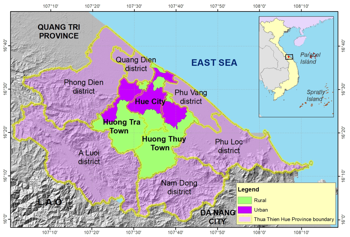
Located in Central Vietnam’s Thua Thien Hue Province, Hue City is a UNESCO-designated heritage urban area that is rapidly urbanizing. In Vietnam and the wider southeast Asian region, the city functions as an important cultural and tourism center. Hue City’s boundaries were expanded through administrative changes in July 2021 to include 29 wards and seven communes, covering a total area of 265.99 km² (Figure 1) [32].

The research area includes the recently expanded city of Hue along with the nearby villages of Huong Tra and Huong Thuy, covering both urban and peri-urban zones. The region experiences a tropical monsoon climate with two main seasons: the RP from September to December, with average temperatures of 20–22 °C, and the LRP from January to August, with average temperatures of 27–29 °C and peak temperatures reaching 38–40 °C in May and June.

The UHI effect has been exacerbated by land-use changes, urbanization, and climate variability, resulting in a decrease in green spaces and an increase in impermeable surfaces. Public health, heritage landscape conservation, and ecological sustainability are all threatened by these dynamics. Thus, in heritage towns like Hue, understanding the spatial temperature fluctuations throughout this mixed urban–rural setting is crucial for climate adaptation and sustainable urban design [33,34,35].

Figure 1. The study area of Hue city, Vietnam [36].

Figure 1. The study area of Hue city, Vietnam [36].

2.2. Satellite Data

2.2.1. Landsat Images

This paper has utilized Landsat satellite data to estimate LST indices in Hue City and the surrounding towns in the LRP and RP seasons from 2000 to 2020. The criterion utilized for data selection was based on the lowest cloud cover percentage, because the Landsat images are optical. The specific Landsat dates were chosen within the period considered (LRP and RP). According to this criterion, the date with the best image quality was taken into consideration. As reported in

Table 1. Landsat dataset used for LST estimation.

Year	Satellite Image (Sensor)	Date of Acquisition	Season	Cloud Cover Land
2020	Landsat 8 (OLI/TIRS)	16 July 2020	LRP	14.8
	Landsat 8 (OLI/TIRS)	2 September 2020	RP	24.1
2010	Landsat 5 TM	5 July 2010	LRP	4.0
	Landsat 5 TM	7 September 2010	RP	48.0
2000	Landsat 5 TM	6 May 2000	LRP	26.0
	Landsat 7 (ETM)	6 November 2000	RP	7.0

, the cloud cover percentage is less than 30% for all the images except for the RP (2010) in which the percentage is more than 30. This is due to the difficulty of finding an optical image for the RP with little cloud cover. Due to the persistent cloud cover during the RP, a drastic masking reduced the temporal resolution of the study period. The selection of the images prioritized those that despite the total footprint cloud cover have the lowest cloud coverage in the Area Of Interest (AOI). In total, eight images of Landsat 5 Thematic Mapper ™, Landsat 7 Enhanced Thematic Mapper Plus (ETM+), and Landsat 8 Operational Land Imager (OLI) and TIRS (Thermal Infrared Sensor) have been used. OLI/TIRS images (Level-1 Data Product) have been acquired from the United States Geological Survey (USGS) Earth Explorer platform [37] with a path/row designation of 125/049 utilized for LST retrieval. The cloud cover land rate in the scenes of the Landsat images ranges from 4% to 48%; however, no cloud was identified/observed in the subset study area. Thus, it is suitable for analyzing the LST by season over 20 years (2000–2020) (Table 1). The thermal band has a 120 m (band 6), 60 m (band 6), and 100 m (band 10, band 11) native spatial resolution for Landsat 5 TM, Landsat 7 ETM+, and Landsat 8 TIRS, respectively, but it was resampled at 30 m by USGS. In spite of the resampling process, there are still limitations in detecting the small-scale thermal anomalies. The recorded LST calculated is an average of different surfaces within the same pixel, but this is not a limit in this thermal analysis, because it is enough to understand which areas are more sensitive to thermal stress.

2.2.2. Sentinel-2 Images

The LULC changes have been evaluated using multispectral imagery acquired by Sentinel-2, which is characterized by its high spatial resolution [38].

Table 2. Sentinel-2 dataset used for LULC and spectral indexes estimation.

Year	Satellite Image (Sensor)	Date of Acquisition	Season	Cloud Cover Land
2024	Sentinel 2A	22 August 2024	LRP	24.1
2022	Sentinel 2A	17 September 2022	RP	8.7
2020	Sentinel 2A	28 August 2020	LRP	9.9
	Sentinel 2A	1 September 2020	RP	31
2016	Sentinel 2A	9 August 2017	LRP	5.2
2017	Sentinel 2A	23 October 2016	RP	39.4

lists the specific Sentinel-2 dataset involved in this research. Being optical images, Sentinel-2 image selection prioritized minimal cloud coverage, which is the same as in the selection of Landsat images.

The imagery, characterized by 290 km and a revisit time of 5 days, comprises 13 spectral bands with spatial resolution from 10 m to 60 m. The Sentinel-2A satellite was launched in June 2015, which is related to the European Copernicus program; it was developed and built under the industrial leadership of Airbus Defence and Space for the European Space Agency (ESA) [39].

The data reported in Table 2, sourced from an open-access web platform [40], encompass the years 2016, 2020 and 2024. As with Landsat images, acquiring scenes with minimal cloud cover proved more challenging for the RP than for the LRP for Sentinel-2 imagery as well. Because it was impossible to find a good image with less cloud cover for all of the years taken into account, the best solution was to consider the year closest to the one that should have been considered.

Given the sensor’s launch in 2015, the initial year of data acquisition for paper was 2016; consequently, it does not temporally align with the Landsat dataset. In Section 3.2, it is possible to identify which bands have been used for the spectral index calculation considering the NDVI, NDWI, and NDBI.

3. Method

The selection of Sentinel-2 imagery, as outlined in Table 2, adhered to a consistent acquisition period of August–September for each of the reference years. This methodological choice, aimed at minimizing the impact of phenological variations, explains why 2025 imagery was not yet included in this paper. Data from the year 2024 represent the most current land cover condition.

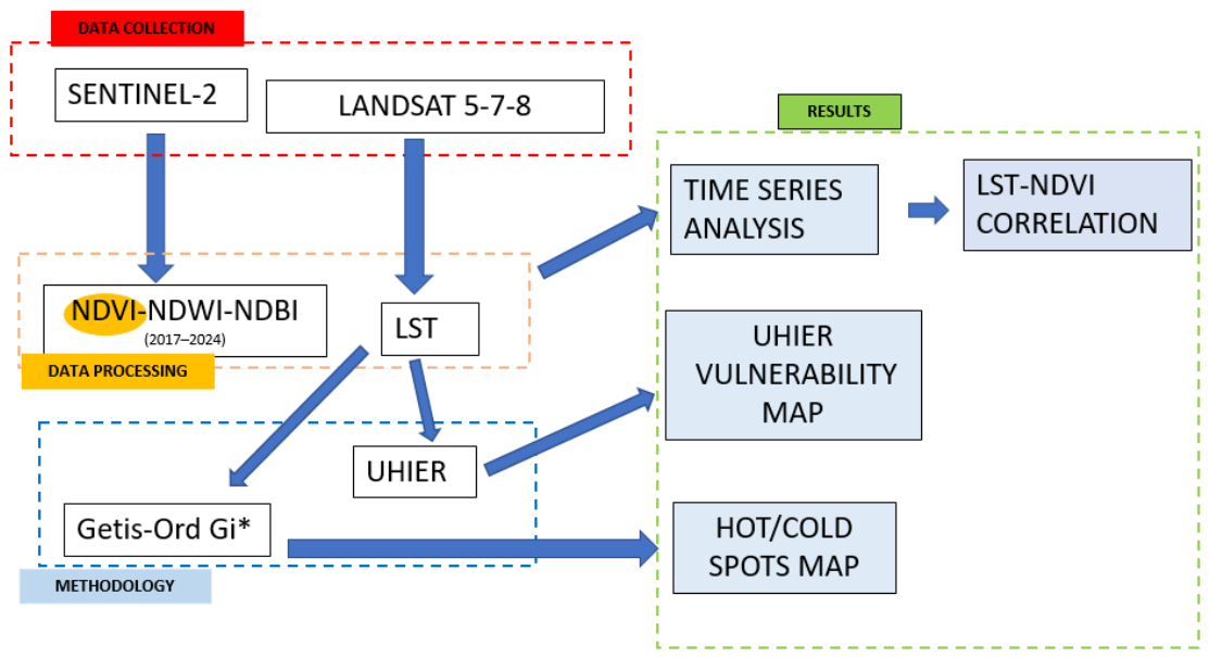
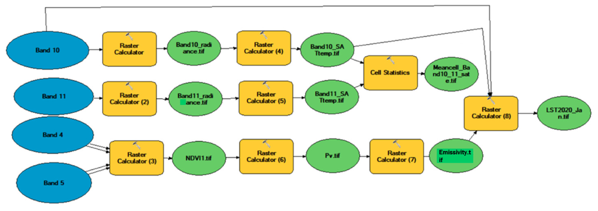
The dataset has been processed in QGIS [41], ArcGIS [42] and Google Earth Engine [43]. Two parallel analytical approaches have been processed considering both thermal analysis and LULC change detection over the years. The thermal analysis served to delineate the extent and intensity of UHIs. The LULC investigation, on the other hand, was fundamental to understand the relationship between specific LULC types and their influence on temperature variations over time. Particular emphasis is placed on the study area (see Figure 1) due to the presence of numerous UNESCO archaeological sites, which are essential for the continuity of historical understanding. The complete methodology applied is illustrated in the workflow reported in Figure 2.

3.1. LST Retrieval from Landsat Images

LST represents the temperature of the Earth’s surface measured by thermal infrared sensors on satellites or aircraft. In this case, thermal sensors on satellite (Landsat satellite) measure it. The thermal parameter finds vital applications in various fields, including UHIs, urban climates, and the cooling effect of urban lakes, as well as agriculture, hydrology and natural hazard monitoring [25,33,34,44,45,46]. Urbanized areas often capture and release solar radiation, leading to higher surface temperatures than adjacent rural regions [25]. The LST is calculated to quantify the temperature in the study area for two seasons in 2000, 2010, and 2020.

This paper estimated LST from thermal infrared bands in Landsat 5 TM (Band 6), Landsat 7 ETM+ (Band 6), and Landsat 8 TIRS (Bands 10 and 11) using the single-channel algorithm (SCA). Without requiring complete atmospheric profiles, the SCA is a popular technique for retrieving LST that uses top-of-atmospheric (TOA) brightness temperature adjusted for land surface emissivity [47,48,49]. Because Band 11 is known to be contaminated by stray light, usually Band 10 is chosen for Landsat 8 [50]. Nevertheless, to reduce the effect of band-specific anomalies, in this paper, the authors considered a mean-based compositing technique between Bands 10 and 11 [47,51,52]. It is recommended that future research prioritize the use of Band 10 or employ correction algorithms when utilizing Band 11 [25,50]. Even when there is a lack of data, this method allows for reliable and consistent LST estimates across various sensors and years.

The main steps for calculating LST are outlined as follows [47,53].

Regarding the spectral radiant, different computations are needed. First, the digital number (DN) of the thermal bands (Band 6) from the Landsat satellite was converted to TOA spectral radiance. For the Landsat 5 TM, Landsat 7 ETM+, the spectral radiance is obtained by

$$L_{\lambda }={\displaystyle \frac{L_{max\lambda }-L_{min\lambda }}{QCA{L }_{max}-QCA{L}_{min}}}\left(QCAL-{QCAL}_{min}\right)+L_{min\lambda }$$

(1)

where $L_{\lambda }$ is the TOA spectral radiance (Watt/(m²·srad·µm)), $QCAL$ is the quantized calibrated pixel value in DN, $L_{min\lambda }$ (Watt/(m²·srad·µm)) is the spectral radiance scaled to ${QCAL}_{min}$, $L_{max\lambda }$ (Watt/(m²·srad·µm)) is the spectral radiance scaled to $QCA{L }_{max}$, $QCA{L}_{min}$ is the minimum quantized calibrated pixel value in DN, and $QCA{L }_{max}$ is the maximum quantized calibrated pixel value in DN. $L_{min\lambda }$, $L_{max\lambda }$, $QCA{L}_{min}$ and $QCA{L }_{max}$ values are obtained from the metadata file of Landsat TM and ETM+ data [47].

In Landsat 8, the spectral radiance value was determined by

$$L_{\lambda }=M_L{Q}_{Cal}+A_L$$

(2)

where $L_{\lambda }$ is the TOA spectral radiance (Watt/(m²·srad·μm)), $Q_{Cal}$ is the pixel value (DN), and $M_L$ and $A_L$ are rescaling coefficients [47].

Regarding the Brightness Temperature (BT), the BT image can be generated by

$$T_B={\displaystyle \frac{K_2}{\ln \left(\frac{K_1}{L_{\lambda }}+1\right)}}$$

(3)

where $T_B$ refers to the effective at-satellite brightness temperature in Kelvin, $K_1$ (Watt/(m²·srad·µm)) and $K_2$ (Kelvin) are the calibration constants, and $L_{\lambda }$ is the spectral radiance [47,54]. The values of the constants ($K_1$ and $K_2$) are presented in

Table 3. Thermal band constants for Landsat 5, Landsat 7, and Landsat 8 [47].

Satellite Images	K1 (Watt/(m2·srad·µm))	K2 (Kelvin)
Landsat 5 (Band6)	607.76	1260.56
Landsat 7 (Band6)	666.09	1282.71
Landsat 8 (Band10)	774.89	1321.08
Landsat 8 (Band11)	480.89	1201.14

.

LST (°C) was determined by

$$LST={\displaystyle \frac{T_b}{1+\left(\frac{\lambda T_b}{\rho }\right)\mathrm{l}\mathrm{n}(\epsilon )}}-273.15$$

(4)

where $\lambda$ is the center wavelength for Band 10 (10.9 μm). $\rho = h·c/\sigma$, where h is the Planck constant (6.626 × 10⁻³⁴ J·s), c is the velocity of light (2.998 × 10⁸ m/s), σ is the Boltzmann constant (1.38 × 10⁻²³ J/K) [47,55], and $\epsilon$ is the land surface emissivity, which can be calculated through (5) and (6):

$$\epsilon =m{P}_V+n$$

(5)

$$P_V=({\displaystyle \frac{NDVI-{NDVI}_{min}}{{NDVI}_{max}-{NDVI}_{min}}}{)}^2$$

(6)

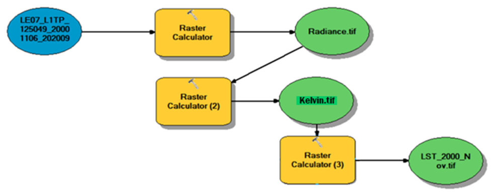
where $P_V$ is the vegetation coverage. The constant values for the emissivity of vegetation and bare soil ($m$ and $n$, respectively) were (calculated as) set to be 0.004 and 0.986, respectively [47,55]. ${NDVI}_{max}$ and ${NDVI}_{min}$ are the study area’s maximum and minimum vegetation indices, respectively. The LST estimation of Landsat 5 TM, Landsat 7 ETM+ and Landsat 8 OLI/TIRS was calculated by the model builder in ArcGIS [51] (see Figure 3 and Figure 4).

It should be noted that Equation (4) does not take atmospheric correction (such as transmittance or upwelling/downwelling radiance) into account; it only takes emissivity correction into account. This simplification is frequently employed in UHI studies when localized atmospheric profiles are not available despite the possibility that it introduces a bias of 1–2.5 °C [47]. Although there is a potential presence of bias, the methodology remains appropriate because the focus is linked to the spatial contrast between the rural and urban area in the surroundings of the CH site. Because the equation is applied in the whole AOI, the UHIER values are statistically correct and give enough information for the thermal vulnerability exposure.

The LST calculation has been used for the intensity index of the UHI (UHIER) calculation [25,56,57,58]:

$$UHIER= {\displaystyle \frac{∆Ti}{Ts}}= {\displaystyle \frac{Ti-Ts}{Ts}}$$

(7)

where $Ts$ is the mean value of LST, while $Ti$ refers to the $i$-th pixel as reported in [25,56,57,58].

Table 4. UHI intensity levels [25,56,57,58].

UHIER	Level
UHIER ≤ 0	Extremely low—0
0 < UHIER ≤ 0.1	Low—1
0.1 < UHIER ≤ 0.2	Medium—2
0.2 < UHIER ≤ 0.3	High—3
0.3 < UHIER	Extremely high—4

indicates five different levels of UHIER intensity. The UHIER value is calculated using (7), and it is crucial for the identification of the factors that influence the presence of UHI. As reported in [59], the UHIER is mostly connected to the accumulation of building material stocks and to the alteration of natural surfaces.

For the sake of completeness, alternative UHI intensity descriptions with respect to (7) [25,56,57,58] are reported in

Table 5. Alternative UHI intensity descriptions [60,61,62,63,64,65] with respect to (7).

Equation	Adopted Terminology	Ref.
$UHIER={\displaystyle \frac{T-T_{min}}{T_{max}-T_{min}}}$	$UHIER$: Urban Heat Island Effect Ratio $T$: LBT (Land Brightness Temperature) $T_{min}$: lowest LBT $T_{max}$: highest LBT	[60]
$UHII={LST}_{urban}-{LST}_{sub}$	$UHII$: UHI Intensity ${LST}_{urban}$: LST in urban areas ${LST}_{sub}$: LST in suburban areas	[61]
$UHII={\beta }_{\mathrm{i}\mathrm{t}}{UFI}_{\mathrm{i}\mathrm{t}}+{\mathsf{\lambda }}_{\mathrm{i}}+{\mathrm{u}}_{\mathrm{i}\mathrm{t}}$	$UHII$: UHI Intensity $UFI$: Urban Form Index $\mathrm{i}$: considered urban area $\mathrm{t}$: considered time ${\beta }_{\mathrm{i}\mathrm{t}}$: slope coefficient ${\mathsf{\lambda }}_{\mathrm{i}}$: fixed effect in the urban area ${\mathrm{u}}_{\mathrm{i}\mathrm{t}}$: residual error	[61]
$UHII={\beta }_1\ln UFI+{\beta }_2\ln UDI+{\beta }_3\ln UFI\ln UDI+\mathrm{u}$	$UHII$: UHI Intensity $UFI$: Urban Form Indicator $UDI$: Urban Development Index $\mathrm{u}$: constant item ${\beta }_1,{\beta }_2,{\beta }_3$: coefficients	[61]
$∆T_i=〈T_{\mathrm{C}i}〉-〈T_{\mathrm{B}i}〉$	$∆T_i$: hourly UHI intensity $〈T_{\mathrm{C}i}〉$: average 2 m air temperature at local time $i$ in the cluster $〈T_{\mathrm{B}i}〉$: average 2 m air temperature at local time $i$ in the boundary	[62]
${SUHII}_i=T_{bui}-T_{gs}$ $SUHII={\displaystyle \frac{1}{n}}{\sum }_{i=1}^n{SUHII}_i$	$SUHII$: Surface Urban Heat Island Intensity ${SUHII}_i$: SUHII at built-up pixel i $T_{bui}$: LST at built-up pixel i $T_{gs}$: mean LST of the green space pixels $n$: total number of built-up pixels	[63]
${UHII}_{urban area pixel}={LST}_{urban area pixel}-{mLST}_{non urban areas}$	$UHII$: UHI Intensity ${UHII}_{urban area pixel}$: UHII in each urban pixel ${LST}_{urban area pixel}$: LST in each urban pixel ${mLST}_{non urban areas}$: mean LST of non-urban areas	[64]
$Composite UHI Index=\mathit{\text{Norm\_LST}}-0.5·\mathit{\text{Norm\_NDVI}}$ $\mathit{\text{Norm\_LST}}={\displaystyle \frac{(LST-\mathrm{m}\mathrm{i}\mathrm{n}(LST\left)\right)}{\left(\mathrm{m}\mathrm{a}\mathrm{x}\right(LST)-\mathrm{m}\mathrm{i}\mathrm{n}(LST\left)\right)}}$ $\mathit{\text{Norm\_NDVI}}={\displaystyle \frac{(NDVI-\mathrm{m}\mathrm{i}\mathrm{n}(NDVI\left)\right)}{\left(\mathrm{m}\mathrm{a}\mathrm{x}\right(NDVI)-\mathrm{m}\mathrm{i}\mathrm{n}(NDVI\left)\right)}}$	$Composite UHI Index$: composite UHI index $\mathit{\text{Norm\_LST}}$: normalized LST $LST$: LST value for each unit $\mathit{\text{Norm\_NDVI}}$: normalized NDVI $NDVI$: NDVI value for each unit	[65]

[60,61,62,63,64,65].

The final stage of the thermal analysis involved the individuation of the hot and cold spots fundamental for the development of mitigation strategies. Knowing where they are located is a prerequisite for implementing cooling actions. This process supports Goal 11 of the Agenda 2030 enhancing urban sustainability and resilience [7,66,67]. Hot and cold spots were individuated based on a statistical approach utilizing the z-score, p-value, and confidence level (

Table 6. The z-score, p-value and confidence level [68,69].

z-Score (SD)	p-Value (Probability)	Confidence Level
<−1.65 or >+1.65	<0.1	90%
<−1.96 or >+1.96	<0.05	95%
<−2.58 or >+2.58	<0.01	99%

). The z-score refers to standard deviation (SD), while the p-value and the confidence level refer to probability. The statistical significance of the z-score is the distance of the SD from the mean value. It gives the information about a point, indicating whether it is unusual with respect is to what is expected. When the z-score value is very high, whether positive or in negative, it says that the confidence level is so high that the point is not random. A small p-value means there is a small probability of observing a result.

3.2. Spectral Indexes Estimation

The NDVI is the most used metric in RS for the quantification of the vegetation area. It is used to quantify the health and the density of the vegetation and uses the near-infrared (NIR) and the red bands. The generic NDVI equation is reported in (8). The specific NDVI equation for Sentinel-2 is expressed in (9). The bands considered are Bands 8 and 4 [70].

$$NDVI={\displaystyle \frac{NIR-Red}{NIR+Red}}$$

(8)

$${NDVI}_{Sentinel-2}={\displaystyle \frac{B8-B4}{B8+B4}}$$

(9)

The NDWI is a metric used in RS for the detection of water bodies. Due to spectral similarities, the NDBI is very reasonable for the urban area and may overestimate the water body extension. It uses the green and the NIR bands. The general NDWI equation is reported in (10) while the specific NDWI equation for Sentinel-2 is expressed in (11), which considers Bands 3 and 8 [71].

$$NDWI={\displaystyle \frac{Green-NIR}{Green+NIR}}$$

(10)

$${NDWI}_{Sentinel-2}={\displaystyle \frac{B3-B8}{B3+B8}}$$

(11)

The NDBI is a metric used to detect the built-up area in order to evaluate the change over time of the LULC to monitor, for example, the urban sprawl. It is used also in the case of environmental impact assessment or for disaster risk evaluation. It is calculated by using the NIR and the Short-Wave Infrared (SWIR) bands, as reported in the following equations:

$$NDBI= {\displaystyle \frac{SWIR-NIR}{SWIR+NIR}}$$

(12)

$${NDBI}_{Sentinel-2}={\displaystyle \frac{B11-B8}{B11+B8}}$$

(13)

To conclude this section, it can be stated that the use of these spectral indices listed above is fundamental for effectively analyzing and monitoring key environmental and urban characteristics using RS data [72].

4. Results

This section provides an overview of thermal and land cover dynamics within the AOI over the years considered. Due to the multi-phase nature of the research, the results are organized in subsequent subsections. The thermal analysis is provided by the LST (see Section 3.1) and by the mapping of hot and cold points. To support the understanding of the AOI (see Figure 1), we needed the identification of an LULC map and its evolution over time.

Three land cover classes (vegetation, water and built) were derived from spectral indices (NDVI, NDWI, and NDBI) using a raster calculator tool. The first step of this phase encountered significant challenges due to the frequent cloud presence within the AOI, excluding numerous satellite images. All the raster products were processed in a GIS environment, specifically the open-source software QGIS and the software ArcGIS. To bypass the problem of low cloud cover satellite imagery availability during the months from September to December, a more time- and year-long analysis was used through the Google Earth Engine free platform.

4.1. LST and UHI Analysis Results

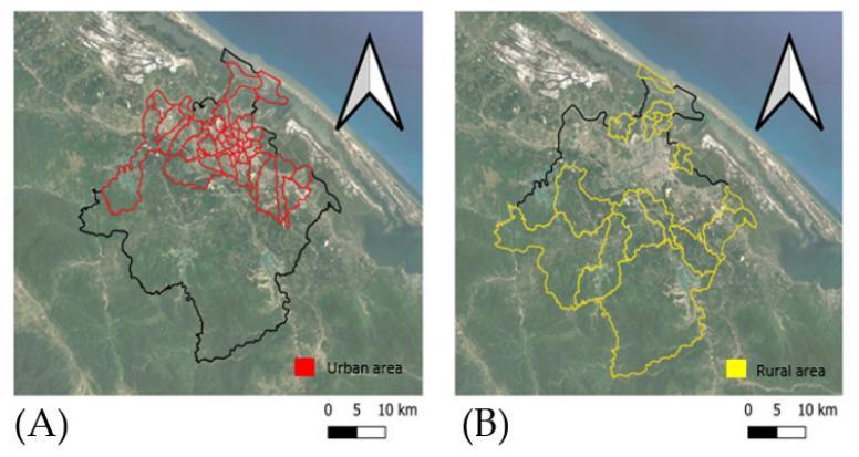
The initial step of this methodology involved the evaluation of the thermal conditions considering two contrasting land cover classes: vegetation and urban. The representation of the urban area is defined through red lines in Figure 5A, while rural areas are represented in Figure 5B through yellow lines. The urban and rural area are delimited not by administrative boundaries but by LULC characteristics. To ensure a more consistence spatial analysis between the two homogeneous classes, an aggregation of districts has been made according to similar land cover properties.

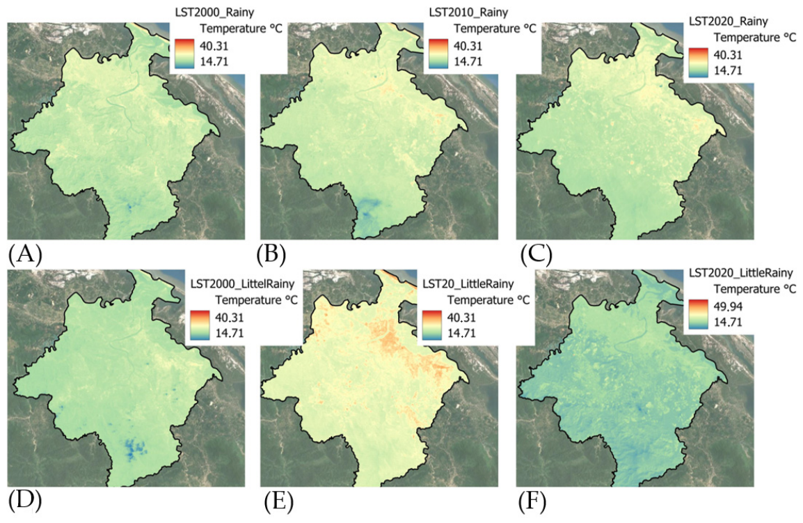
The LST has been calculated for the years 2000, 2010 and 2020 for both the LRP and the RP.

All the LST raster calculations are reported in Figure 6A–F. The top row Figure 6A–C represents the LST during the RP (in particular, 2000 (Figure 6A), 2010 (Figure 6B), and 2020 (Figure 6C)). The bottom row Figure 6D–F represents the LST during the LRP (in particular, 2000 (Figure 6D), 2010 (Figure 6E), and 2020 (Figure 6F)).

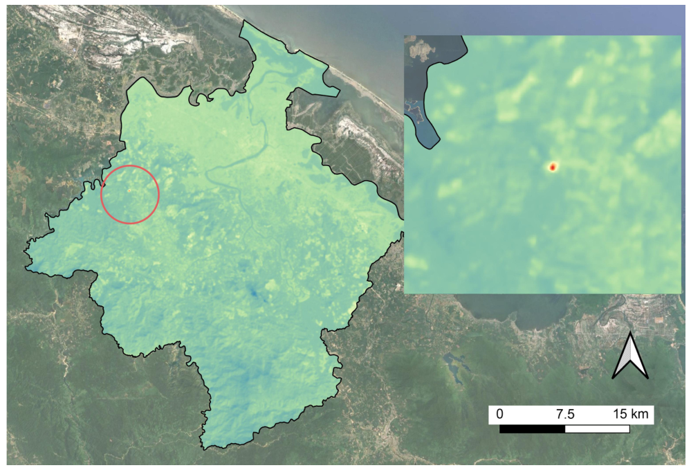
To detect possible outliers in the dataset, the neighborhood of each point was analyzed to determine its associated mean temperature. If the computed mean temperature of the considered point area’s neighborhood differs too much from the temperature of the point area, an outlier is detected. The same algorithm was applied for all the satellite images considered. The 50 °C spike in the 2020 LRP (Figure 7) was identified as a radiometric anomaly and as a non-physical artifact. For instance, it has been excluded to ensure the statistical integrity of the UHIER.

Two values have been considered as a range of minimum and maximum values for all the LST representations.

Table 7. Statistical analysis of the LSTs.

Year	Season	Mean Value (°C)	Min Value (°C)	Max Value (°C)	SD (°C)
2000	LRP	22.32	16.17	49.93	1.30
	RP	23.24	14.92	34.53	1.49
2010	LRP	26.55	22.81	40.31	1.60
	RP	24.25	15.17	34.46	1.63
2020	LRP	22.33	18.92	30.60	1.31
	RP	23.61	18.41	32.08	1.68

presents the statistical information for the LST across the period considered, illustrating the evolution of temperature values and highlighting the progressive increase in thermal heterogeneity. It corresponds to the localized urban growth identified in the LULC analysis reported in Section 4.3.3. The transition from a uniform to fragmented mosaic of residential and rural areas increased the contrast between adjacent pixels and the SD values.

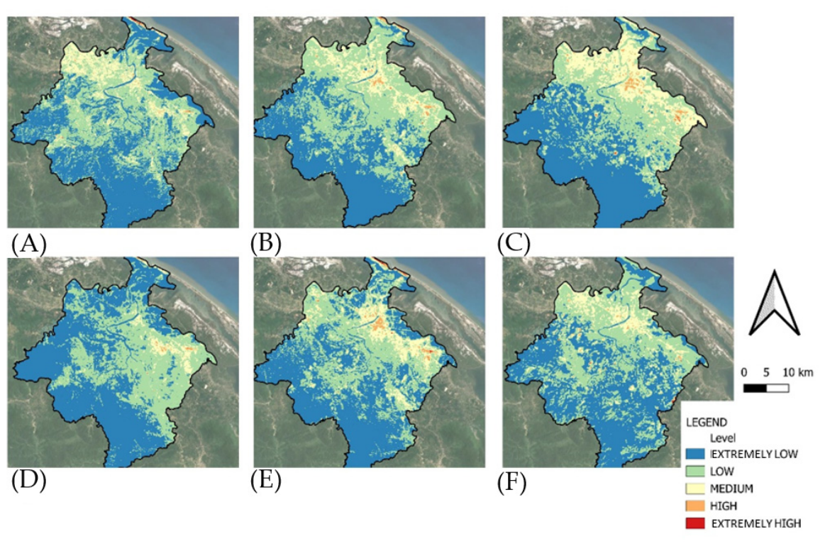
The geospatial representation of the UHIER over time and season is illustrated in Figure 8, while the UHIER statistical values are summarized in

Table 8. Statistical analysis of the UHIER maps.

Year	Season	Mean Value	Min Level	Max Level	SD
2000	LRP	0.58	0	4	0.48
	RP	0.62	0	4	0.69
2010	LRP	0.62	0	4	0.72
	RP	0.70	0	4	0.70
2020	LRP	0.60	0	4	0.66
	RP	0.74	0	4	0.79

.

Figure 8 shows the UHIER over the years in both the RP and LRP. The first row contains the representations of the RP of the year 2000 (see (A)), 2010 (see (B)) and 2020 (see (C)). In the second row of the image matrix, there are the representations of the LRP for the year 2000 (see (D)), 2010 (see (E)) and 2020 (see (F)).

The percentage of the total area corresponding to each level of UHI is reported in

Table 9. UHIER percentage (%) evaluation over the LRP and RP.

Level	2000R	2000LR	2010R	2010LR	2020R	2020LR
Extremely low	49.12	55.82	43.08	50.42	46.44	48.98
Low	39.87	40.13	44.64	38.02	34.31	41.99
Medium	10.39	3.71	11.37	10.10	17.84	8.53
High	0.48	0.34	0.86	1.32	1.40	0.45
Extremely high	0.14	0	0.06	0.13	0.02	0.05

to conduct a quantification assessment. A comparison between the RP and LRP for each year considered is reported in Table 9. The percentage distribution of the UHIER across 2000–2010–2020 for the RP and LRP is consistent with the pattern spatial distribution represented in Figure 8. A dominance of the UHI “extremely low level” is notable, highlighting that they are primarily located in the inner area of the study area.

As an additional step, a temporal variation analysis of the LST was conducted by making a pairwise comparison of years within the same season (LRP or RP). The classification of the difference between two years considered for each calculation is reported in

Table 10. LST relationship.

LST Difference	Category
LST < 0	Increasing
LST = 0	No difference
LST > 0	Decreasing

. When the difference is equal to zero (LST = 0), it means that there is no difference. When there is a negative difference value (LST < 0), it means that there is an increase in the temperature; on the contrary, when there is a positive difference value (LST > 0), there is a decrease in the temperature.

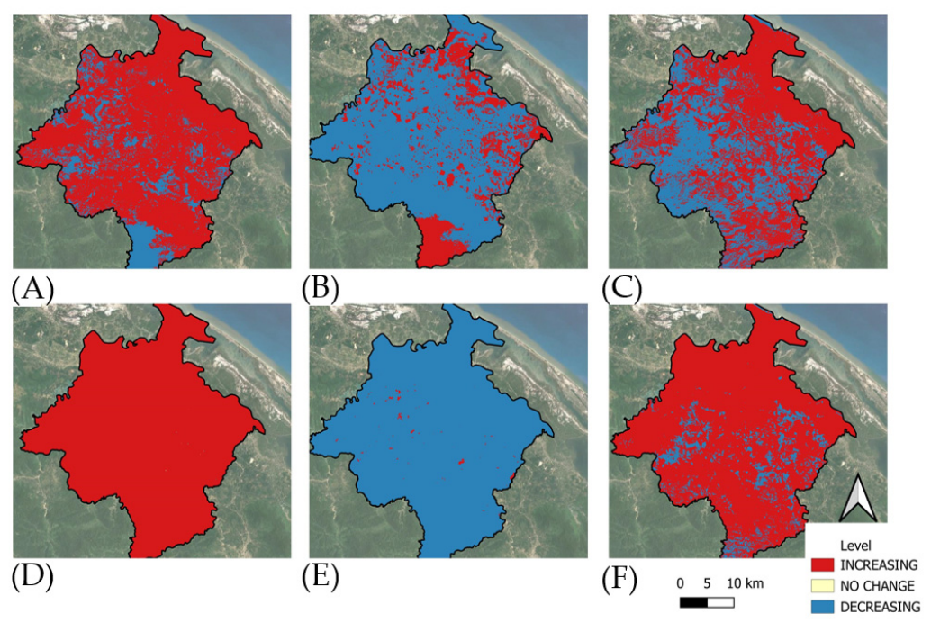
The pattern spatial distribution of LST is shown in Figure 9 that is composed of two rows representing the two different seasons. The first row of the matrix image represents the RP differences between the years 2000–2010 (see (A)), 2010–2020 (see (B)), and 2000–2020 (see (C)). The second row of the image matrix represents the LRP differences between the years 2000–2010 (see (D)), 2010–2020 (see (E)), and 2000–2020 (see (F)).

The LST pattern spatial distribution depicted in Figure 9 is quantitatively represented in

Table 11. The RP and LRP area percentage (%) evaluation.

LST Difference	LST 2000-2010RP	LST 2000-2010LRP	LST 2010-2020RP	LST 2010-2020LRP	LST 2000-2020RP	LST 2000-2020LRP
Increasing	80.76	99.99	23.36	0.47	58.12	88.73
No differences	0.00	0.01	0.00	0.00	0.00	0.00
Decreasing	19.24	0.00	76.64	99.53	41.88	11.27

, according to the LST relationship categories defined in Table 10.

4.2. Hot and Cold Spot Analysis Results

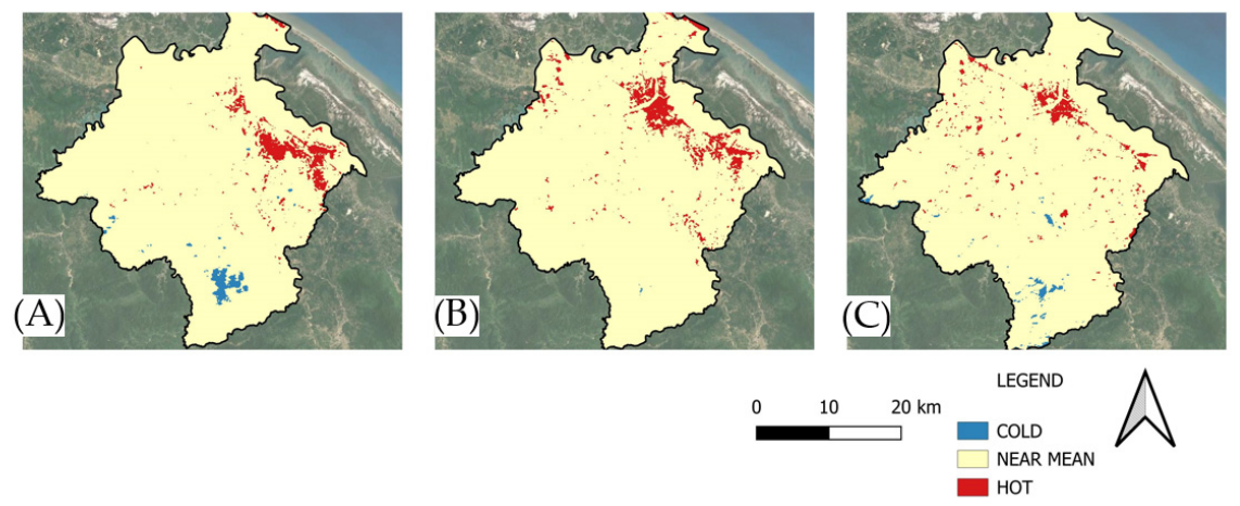
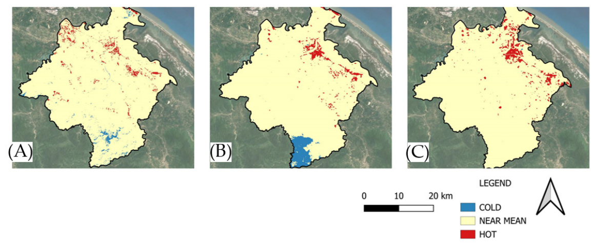
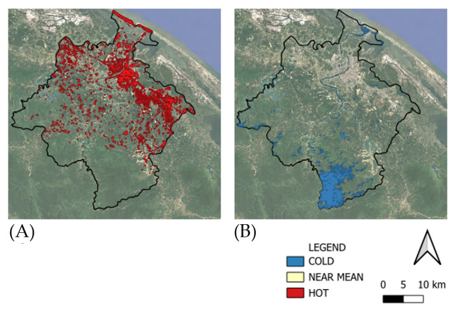
The identification of hot and cold spots is fundamental for thermal analysis, enabling the identification of areas with greatest need for urban regeneration or green areas. To analyze the temporal evolution of these thermal extremes, their trend was evaluated across the years. To investigate the dynamics of the hot and cold spots in both the LRP and RP, their geospatial representation is shown in Figure 10 and Figure 11. Figure 10 shows the dynamic variation for LRP of the hot and cold spots across the years, following this order: 2000 (see (Figure 10A)), 2010 (see (Figure 10B)), and 2020 (see (Figure 10C)). Figure 11 shows the dynamic variation for the RP of the hot and cold spots across the years following this order: 2000 (see (Figure 11A)), 2010 (see (Figure 11B)), and 2020 (see (Figure 11C)).

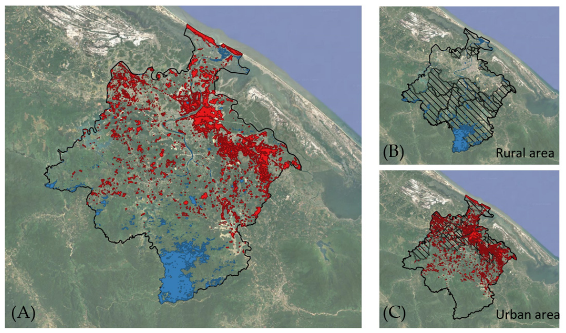
A synthesis of geospatial analysis of Figure 10 and Figure 11 is illustrated in Figure 12 with the spatial intersection of all hot and cold points identified over the years. Figure 12A highlights that hot spots are predominantly concentrated in the urban area; conversely, Figure 12B shows that cold spots are mainly situated in rural areas, where the vegetation presence facilitates lower surface temperatures.

Figure 13 provides a validation of the output explained in Figure 12. The merged spatial overlap between the administrative/land-cover delineations and the identified thermal clusters is a high spatial correlation confirmation. The coldest points are represented in the rural zone (Figure 13B), while the hottest points are within the urban core (Figure 13C).

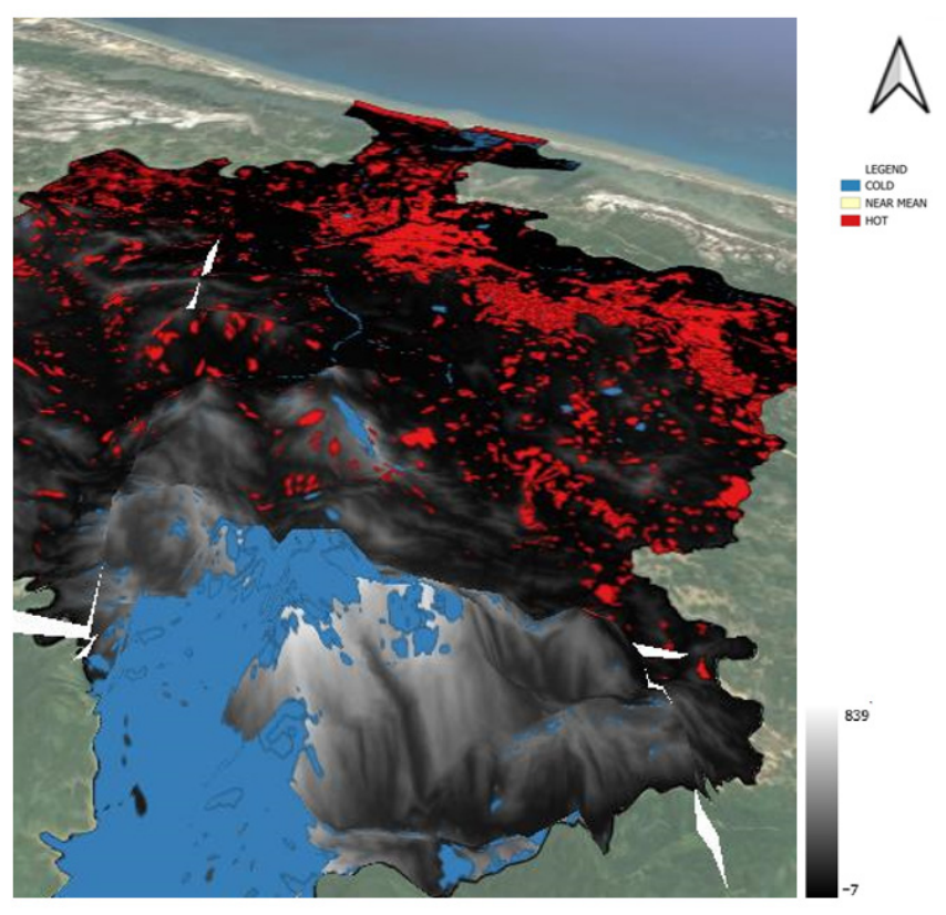
Figure 13A is the merged points representation composed by the total amount of hottest and coldest points over the years analyzed by a statistical method reported in Section 3.1 and Table 6. Its 3D representation using the Shuttle Radar Topography Mission (SRTM) data is represented in Figure 14. Also, this representation confirms the presence of the coldest points in the highest part of the area of study. The necessity of developing mitigation actions to effectively manage this temperature intensification issue is quite urgent.

4.3. Spectral Index Analysis Results

Sentinel-2 multispectral optical images were used to enhance the understanding of the Than Thien Hue Province study area over the past three decades. The primary source of heat generation is anthropogenic and urban activity coupled with progressive soil sealing, strongly increasing the phenomenon. A diachronic analysis of land cover is essential to establish mitigation actions to restrict the UHI and its effects. The dataset used for this analysis is reported in Table 2.

The raster images were processed in a GIS environment through free software, QGIS. The multi-sensor analysis depends on the spatial resolution. Landsat imagery has lower resolution than Sentinel-2 imagery. Although the other multispectral bands feature has a resolution of 30 m (coarser than Sentinel-2), the native Landsat thermal band has a resolution of 100 m. Three different years, one for each decade, were considered to assess the change over time. Because the launch of the Sentinel sensor is much more recent than that of the Landsat sensor, the years considered for the Sentinel-2 analysis are different from the years considered for the thermal analysis.

The raster spectral indices calculated (NDVI, NDWI, and NDBI) have been described in Section 3.2. Their values range from −1 to +1. Respectively, when the value is very close to +1, it means that the area has a lot of vegetation, body water, or high urban density. Conversely, when the value is −1, there is an absence of vegetation, body water, or urban density. Due to the high spectral similarity between water and urban areas, the detection phase may lead to an overestimation of water bodies.

4.3.1. NDVI

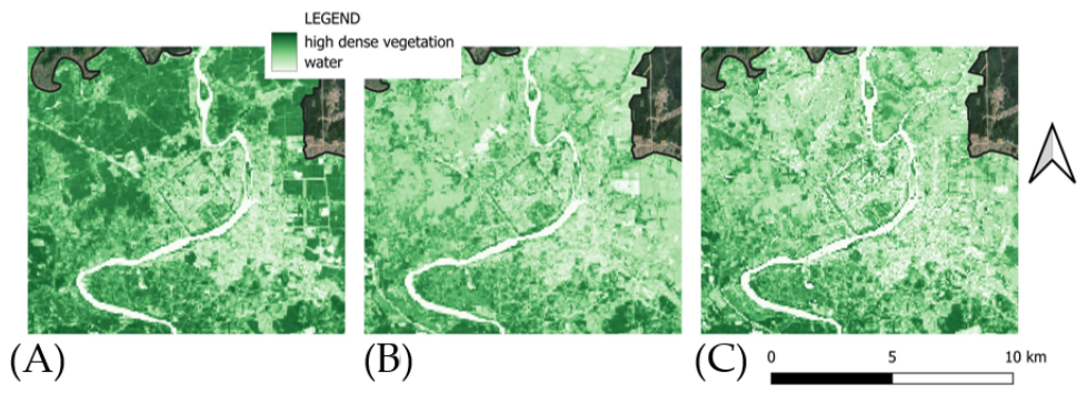
The NDVI is the most used spectral index for monitoring and quantifying the vegetation as well as for assessing vegetation health. The classification of the NDVI is based on four classes, as reported in

Table 12. NDVI range classification.

Class	Pixel-Value
Water	<0
Soil	<0.4
Low dense vegetation	<0.6
High dense vegetation	<1

. According to Table 12, when the pixel value is around 0, the vegetation assumes a stressed aspect and show very low density, or it is soil. Concerning that classification, Figure 15 illustrates how the water body is represented with the lowest range of classification. There are many NDVI applications in the field of crop monitoring or biomass estimation. In this paper, it is used as support to determine how the land cover changes over time. Indicatively for vegetation index evaluation, it is best to consider a non-dry period. In fact, for Section 4.3, the period considered was only the LRP. As reported above, the AOI of this paper is very often covered by clouds, so the capture of the data collection was very complicated.

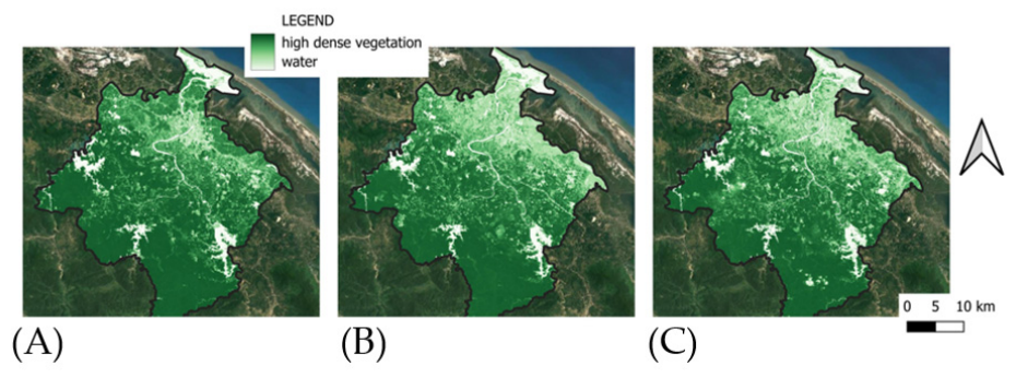
The NDVI in the LRP is shown in Figure 15 in the following order: 2017 (Figure 15A), 2020 (Figure 15B), and 2024 (Figure 15C). The central urban area suffered low/high dense vegetation reduction over the years (see Figure 16). A zoomed-in view of the AOI is represented in Figure 16.

Table 13. NDVI statistics value over the years 2017, 2020, and 2024.

Year	Mean Value	Min Value	Max Value	SD
2017	0.69	−0.98	0.96	0.31
2020	0.65	−0.58	0.92	0.29
2024	0.63	−1	0.94	0.36

presents the statistical values of the NDVI raster during the LRP. While the mean NDVI value decreased, the SD increased, which suggests a greater spatial heterogeneity in vegetation health. In 2024, the minimum value reaches −1; that does not occur in the previous years considered. In 2024, the maximum value instead decreases, so it means that the concentrations of a good healthy vegetation have been compromised by some factors. In 2020, the minimum value was not low, so probably the conditions were a bit more natural from the following year considered. The vegetation index evaluation was processed in the Google Earth Engine platform.

4.3.2. NDWI

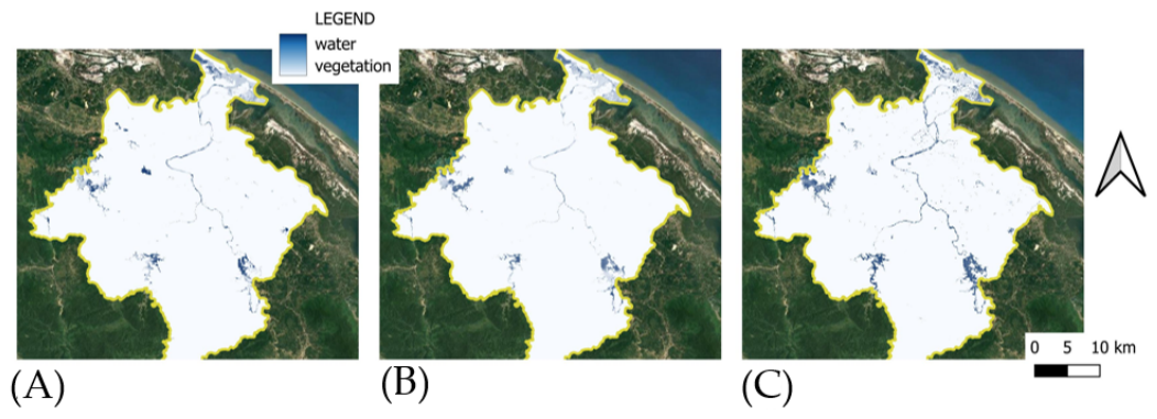
The NDWI could be the best water index used in the RS field to evaluate the change in the water body presence in a time series analysis. According to this issue, a binary classification has been carried out (see

Table 14. NDWI range classification (binary classification).

Class	Pixel Value
no water/vegetation	<0
water	<1

). In Figure 17, the representation of the water body is reported in blue together with its variations.

The NDWI mean values reported in

Table 15. NDWI statistics value over the years 2017, 2020, and 2024.

Year	Mean Value	Min Value	Max Value	SD
2017	−0.60	−0.89	0.99	0.29
2020	−0.58	−0.82	0.81	0.27
2024	−0.56	−0.88	1	0.34

show a decrease in the value, while the minimum value increases from 2017 to 2024; the same behavior holds for the maximum value. Also, the SD shows the same trend, passing from 0.29 to 0.34 and reaching an increase of 17.24%.

4.3.3. NDBI

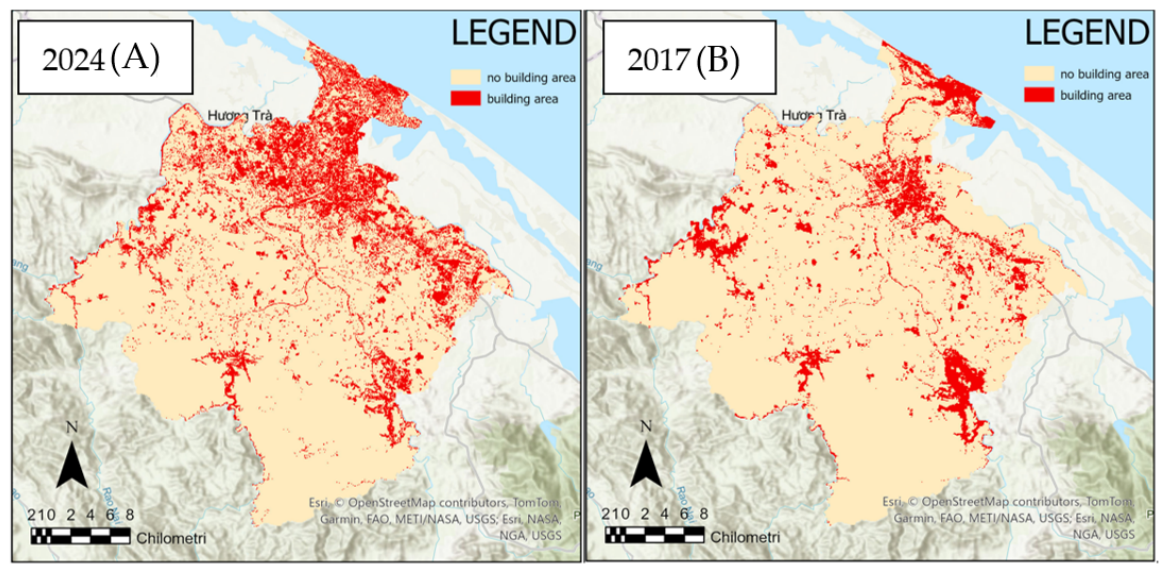
The NDBI calculation is used to evaluate how the building area increases in a region of interest. It is possible to have an overestimation of the building area due to the presence of water as reported in Figure 18. However, in spite of this, it is evident how the building part defined in red has increased over the years.

4.3.4. Google Earth Engine Processing

For the RP, high cloud cover across several scenes made the selection of individual annual images unfeasible. To perform a longer period assessment from 2019 to 2024, the data were processed in Google Earth Engine. The GEE platform facilitated the identification of the spectral indices (NDVI, NDWI and NDBI) trends over the years.

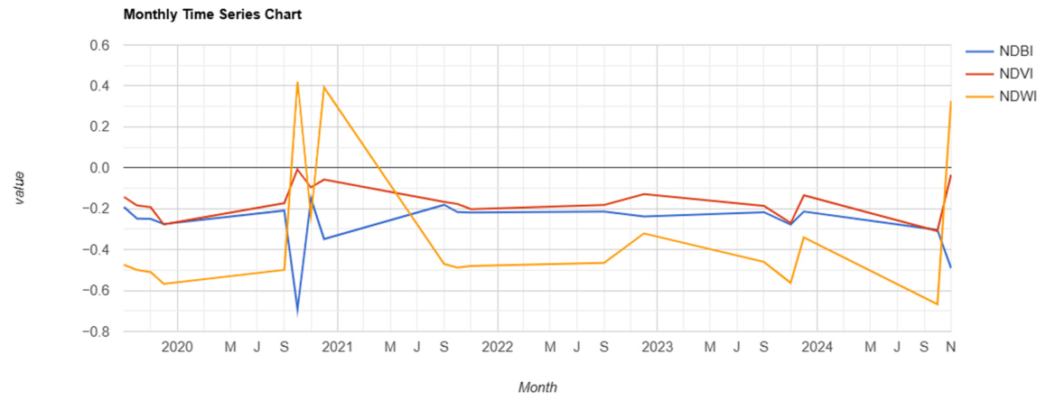
Figure 19 illustrates the monthly spectral indices trends from 2020 to 2024: NDVI (red line), NDWI (yellow line), and NDBI (blue line). The critical values exploited in the charts are conformed to events registered on the Copernicus Emergency platform.

Generally, the NDVI and NDWI trends are affected by natural events and seasonal fluctuations. Statistical peaks often coincide with critical events.

4.4. Results of the Correlation Between the LST and the NDVI

To investigate the existence of a linear correlation between the NDVI and LST, four Landsat images were considered: two for the LRP and two for the RP (years 2020 and 2024; see

Table 16. Landsat images for LST/NDVI correlation.

Year	Path/Row	Landsat Image	Date of Acquisition	Season	Cloud Cover
2024	125/049	Landsat 9 (OLI/TIRS)	4 August 2024	LRP	28.55
2023	125/049	Landsat 8 (OLI/TIRS)	19 September 2023	RP	15.63
2020	125/049	Landsat 8 (OLI/TIRS)	16 July 2020	LRP	13.92
	125/049	Landsat 8 (OLI/TIRS)	2 September 2020	RP	22.17

). This was important to make two considerations: if the correlation changed over the seasonality and if the correlation changed from 2020 to 2024.

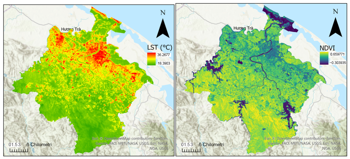
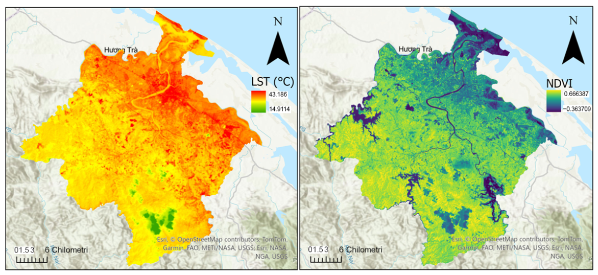
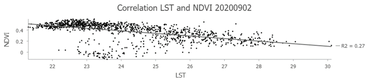
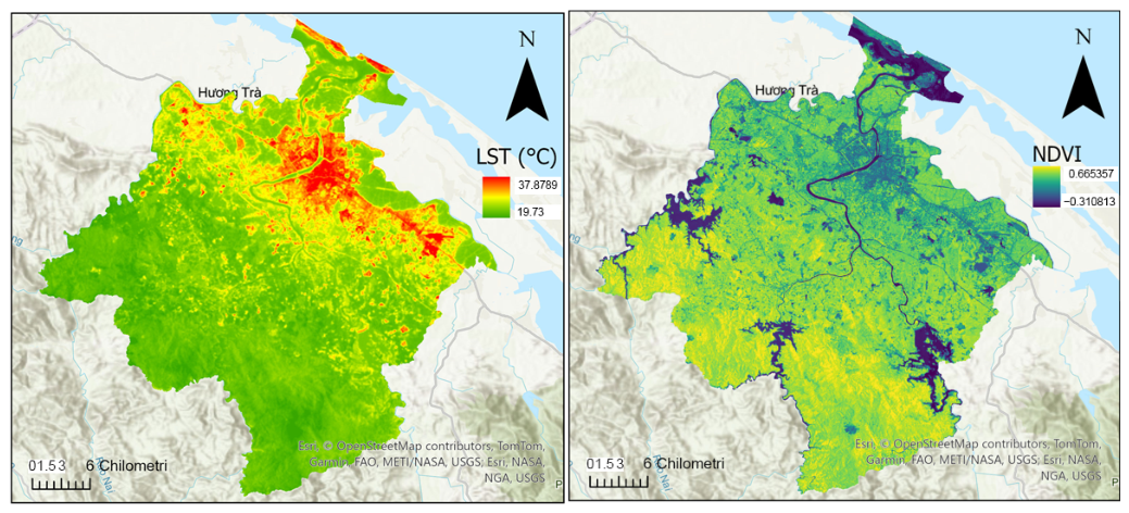
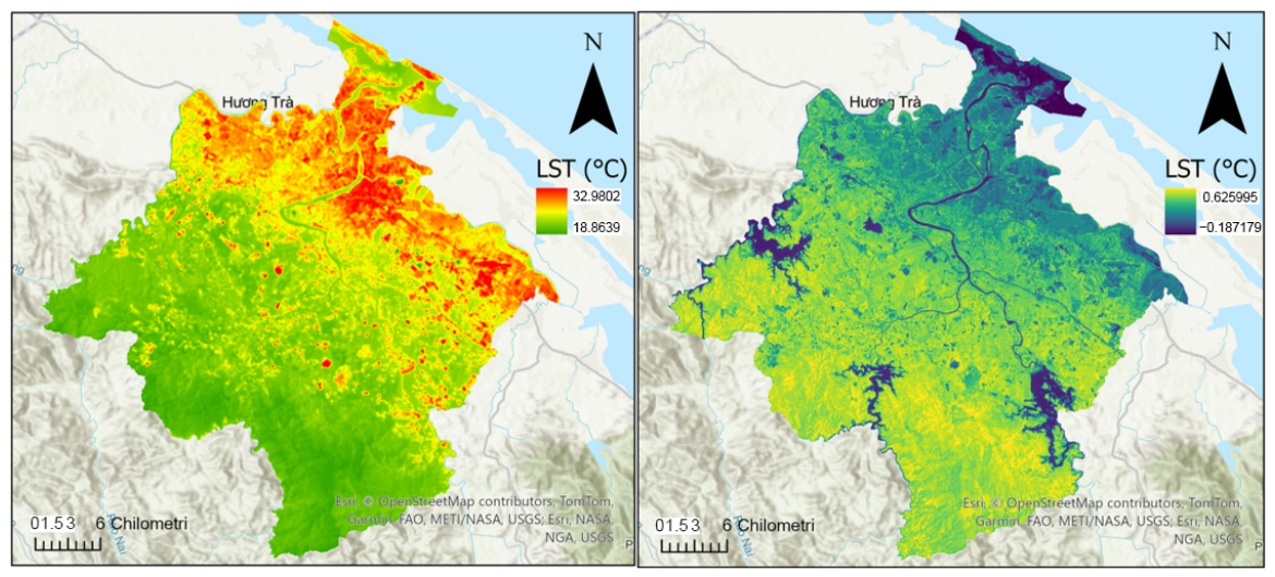
Figure 20, Figure 21, Figure 22 and Figure 23 represent the LST and the NDVI evaluation of the LRP for 2024 and 2020, the RP for 2023, and the RP for 2020.

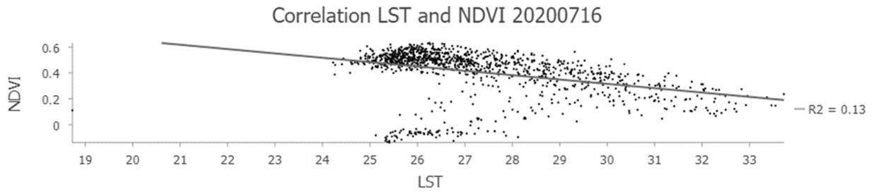
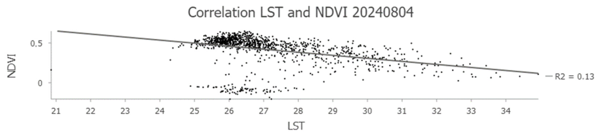
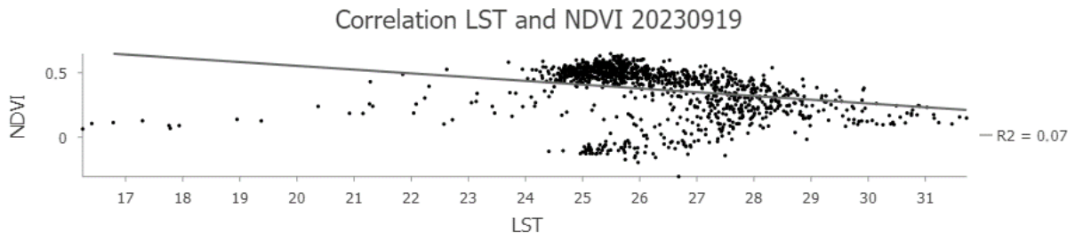
The LST/NDVI correlation for the LRP in 2024 and 2020 reported in Figure 24 and Figure 25 provided a R² = 0.13. For the RP, the correlations are reported in Figure 26 and Figure 27 with a decrease in the R² value from 2020 (R² = 0.27) to 2024 (R² = 0.07). In these figures, the y-axis represents the NDVI, while the x-axis represents the LST. The angular coefficient is negative; it means that when a value increases, the other decreases but with not a strong consistency, as shown by the R² values.

5. Discussion

5.1. LST and UHI Analysis

As can be observed in Figure 6 and Figure 7, as well as Table 7 (see Section 4.1), the highest LST value was recorded in the LRP of 2010 (40.31 °C), while the lowest temperature was recorded in the LRP of 2000 (14.71 °C). In 2000, during the RP, the mean value of LST was 23.24 °C with a minimum temperature of 14.92 °C and a maximum of 34.53 °C. During the LRP, the mean value of LST was 22.17 °C with a minimum of 14.71 °C and a maximum of 29.60 °C. In 2010, the RP had a mean value of LST of 24.25 °C with a minimum of 15.18 °C and a maximum of 34.46 °C. During the LRP, the mean value of LST was recorded at 26.55 °C with values ranging from a minimum of 22.82 °C to a maximum of 40.31 °C. In 2020, during the RP, the mean LST was 23.61 °C with a minimum of 18.41 °C and a maximum of 32.08 °C. The LRP, adjusted for an outlier in the dataset, had a mean LST of 22.33 °C with a minimum of 18.93 °C and a maximum of 30.61 °C. The maximum value for this period was accustomed due to an outlier (49.94 °C) in the original data, as reported in Figure 6F. The SD value increases for the RP increasing from 1.49 °C for 2000 to 1.68 °C for the RP in 2020. For the LRP, instead, the variation is higher, increasing from 2000 to 2010 and from 2010 to 2020. For 2000 and for 2020, the values are nearly identical. The SD value indicates how the LST value is far from the mean value. Significant spatial patterns are indicated by the SD values’ temporal progression. Growing thermal heterogeneity is evidenced by the increasing SD, which highlights wide disparities between built-up centers and vegetated or water-covered outlying areas (from 1.30 °C in the 2000 LRP to 1.68 °C in the 2020 RP). These findings are aligned with urban thermal studies conducted in tropical climates, where surface heat divergence is amplified by fast development and spatial fragmentation.

With regard to the UHIER, Table 8 demonstrates that the mean UHIER value is generally higher during the RP if compared to the mean UHIER values of the LRP (see Section 4.1). Moreover, there seems to be an increasing trend in this value over the years, going from 2000 to 2020. The minimum level is zero for all the years investigated. This shows that at least it would be an “extremely low-intensity level” condition. The maximum level is the same for both the RP and LRP, and it is recorded with a value of 4. It means there are some sub-regions in the AOI where there is the possibility of “extremely high intensity level” conditions. Regarding the UHIER SD values, that measures the variability of the UHIER intensity; it is evident how the RP exhibits a higher SD value than the LRP. Over the trends across the seasons (LRP and RP) and the years (2000–2010–2020), it assumes a slight fluctuation.

In Figure 8, it is visible how the greater part of the AOI is covered by the UHI “Extremely low-intensity level”. Certainly, the course of the river is characterized by the UHI “extremely low-intensity level”. This is probably attributable to the mountainous geo-morphology and to the presence of the rural area depicted in Figure 5B. The open green space allows for heat dissipation, guaranteeing the presence of a “normal” temperature [59,73]. The presence and the applications of blue–green actions used as mitigations for the UHI reduction indicate a cooling effect [74,75]. It reduces the presence of heat in the urban area, guaranteeing better livability and health quality. However, there are areas where there is a high level of UHI depicted in orange. Mainly, this is in areas where there is an urban center, as shown in Figure 5A. As one moves away from the urban center, one can see how the intensity level of the UHI is decreasing to reach a medium level.

In Table 9, it can be noticed that in 2000, during the RP, 49.12% of the study area was classified as Extremely Low UHI, indicating a relatively low UHI effect. Low UHI covered 39.87%, suggesting that most of the study area still experienced mild UHI effects. A smaller portion of the area was classified as Medium UHI (10.39%) or High UHI (0.48%), while extremely High UHI was rare, occurring in just 0.14%. During the LRP, in 2000, Extremely Low UHI was the dominant category, covering 55.82% of the region, while Low UHI was present in 40.13%. Medium UHI was found in just 3.71%, and higher UHI categories (High and Extremely High) were virtually absent. In 2010, during the RP, Extremely Low UHI was observed in 43.08% of the study area with Low UHI covering 44.64%. The proportion of Medium UHI increased slightly to 11.37%, and High UHI remained low at 0.86%. High UHI decreased to 0.06%. During the LRP in 2010, Extremely Low UHI decreased to 48.98%, and Low UHI remained dominant at 41.99%. A slight increase in Medium UHI to 8.53% was observed, while High and Extremely High UHI remained minimal at 0.45% and 0.05%, respectively. In 2020, during the RP, Extremely Low UHI decreased to 46.44%, and Low UHI decreased to 34.31%. The proportion of Medium UHI raised significantly to 17.84%, while High UHI increased to 1.40%. Extremely High UHI remained very small at 0.02%. During the LRP in 2020, Extremely Low UHI remained the dominant category at 48.98% with Low UHI at 41.99%. Medium UHI saw a slight increase to 8.53%, while the higher UHI categories (High at 0.45% and Extremely High at 0.05%) remained negligible.

From 2000 to 2010, during the LRP, nearly the entire study area (99.99%) exhibited an increase in LST with no areas experiencing a decrease (see Table 10 and Table 11; Figure 9). In the RP, for the same interval, 80.76% of the area showed an increase in LST, while 19.24% experienced a decrease. Between 2000 and 2020, LST increased across 88.73% of the study area during the LRP with 11.27% showing a decrease. In the RP, 58.12% of the area showed an increasing LST, while 41.88% experienced a decrease in LST. For the period from 2010 to 2020, the LST increased in only 0.47% of the area during the LRP, while the majority (99.53%) exhibited a decreasing LST. Similarly, during the RP, 23.36% of the area experienced an increase in LST, while 76.64% showed decreasing LST.

The absence of atmospheric correction in LST retrieval is one of this paper’s methodological limitations. The known stray light problem in Band 11 remains a concern even though both Bands 10 and 11 were utilized and averaged to reduce sensor noise. When high thermal accuracy is required (e.g., MODTRAN, MODIS-LST, or reanalysis data (e.g., ERA5-Land)) for cross-validation, future research should use Band 10 exclusively or incorporate sophisticated atmospheric correction models. Band 10 should be used specifically when working with Landsat 8. Notwithstanding these drawbacks, the temporal and spatial trends noted remain strong and helpful in planning and monitoring UHIs.

Recent research has shown that combining Landsat 8 TIRS Bands 10 and 11 enhances LST retrieval in heterogeneous atmospheric conditions, which lends credence to our approach. The generalized split-window (GSW) algorithm makes use of both bands to account for changes in atmospheric absorption and radiometric noise, providing better LST accuracy in a variety of landscapes [52]. Additionally, in [48], the authors demonstrated that the split-window algorithm employing Bands 10 and 11 performs better than single-channel methods, especially in situations where localized atmospheric correction is not available. In order to improve radiometric stability, we used a simplified averaging technique between Bands 10 and 11 in conjunction with outlier filtering, even though we were unable to apply the entire GSW algorithm because there were no concurrent water vapor profiles.

5.2. Hot and Cold Spot Analysis

As can be noticed in Figure 10 and Figure 11 (see Section 5.1), for the LRP, the trend in the number of hot spots is not linear; rather, it appears there was an increase between the year 2000 and the year 2010, which was followed by a decrease from 2010 to 2020. Conversely, regarding the cold spots during the LRP, there was a decrease in their number from 2000 to 2010 and a slight increase from 2010 to 2020. Therefore, in the year 2020 for the LRP, we have an intermediate situation in terms of the number of both hot and cold spots compared to the other two years. For the RP, however, the condition is slightly more evident. The density of hot spots shows a consistent increase, concentrating particularly in the urban area of the study region. Conversely, for the cold spots during the RP, there is a significant increase between 2000 and 2010, showing a notable and evident concentration of points in the bordering area of our study region. This is then followed by a similarly evident decrease in these points between 2010 and 2020.

5.3. Spectral Index Analysis

With regard to the NDVI (see Figure 15 and Figure 16), the increase in areas colored light green may indicate urban growth around the heritage UNESCO Citadel of Hue that must compromise its long resilience. It exposes the archeological sites to being vulnerable to many natural risks such as the flood. Another risk, that is the focus of this research, is the presence of the UHI given from the non-dissipation of the building materials. In addition, observing Table 13, an increase in the SD can be noticed. This increase ensures that the inhomogeneity of land cover over the years increases, making the management of the territory more complex.

With regard to the NDBI (see Figure 18), since there is no difference in building detection between seasons, only one annual index evaluation was made. To better highlight the rapid urban growth over a relative short period, the analysis focuses on the year 2017 and 2024 (Figure 18A,B). This assessment should give rise to concern and an urgency to set mitigation standards in compliance with the climatic conditions.

In addition, NDVI, NDWI and NDBI evaluation has been processed exploiting the Google Earth Engine platform (see Figure 19). For NDVI, a decrease in its value is registered from December 2020 to November 2021, from December 2022 to September 2023 and from December 2023 to October 2024 where there is the lowest value. The positive peaks are in October 2020 and in November 2024. As can be observed in Figure 19, the NDWI registered three very high peaks over the years considered. The first peak is in October 2020, decreasing in November 2020; the second peak is in December 2020, descending until September 2021, maintaining a constant value for 12 months. The last peak is registered in November 2024. The peak of October 2020 is confirmed and probably is correlated to the natural event (storm) of the 7th of October registered in Copernicus Emergency [76]. A flood event is registered on 15 October 2020 due to a storm episode [77]. In [78], it is possible to download the precipitation data of the entire country from 2024. Comparing the precipitation of September, October and November 2024, the highest concentration precipitation in consecutive days is in November. If these concentrations refer to the Province of Thua Thien-Hue [79], this would justify the NDWI peak. As can be observed in Figure 19, the NDBI has a quite constant trend. Its negative peaks are recorded in the same time as the positive peaks of the NDWI index.

5.4. Correlation Between the LST and the NDVI

With regard to the correlation analysis between the LST and the NDVI (see Figure 20, Figure 21, Figure 22 and Figure 23), although there is a year’s difference between the two periods (LRP of 2024 and RP of 2023) considered, what is remarkable is how the temperature dispersion changes over the transition between one season and the next. For the LRP (4 August 2024), the minimum and maximum value were 19.73 °C and 37.87 °C with a mean value of 27.12 °C and an SD of 1.72 °C. For the RP (19 September 2023), the minimum and maximum value were 14.91 °C and 43.18 °C with a mean value of 26.27 °C and an SD of 1.7 °C. The mean value is quite similar, but the extreme temperatures probably increased due to the seasonality. The same analysis was conducted almost three or four years before the previous test. It is possible to note that the trend is confirmed as negative. The minimum values are 18.39 °C for the LRP in 2020 and 18.86 °C for the RP in 2020, while the maximum values are, respectively, 36.26 °C and 32.98 °C. The SD is 1.88 °C for the LRP and 1.76 °C for the RP.

For the LRP in 2024 and 2020 (see Figure 24, Figure 25, Figure 26 and Figure 27), the correlation is very weak. It is also weak for the RP, where the correlation is close to zero. For the RP of 2024, the correlation is less weak than that in 2020. This analysis reveals that the health of vegetation does not depend on the surface temperature.

5.5. Further Considerations

This paper utilized a methodology that is able to monitor and mitigate the UHI effects on a CH site that is affected by a fast urbanization in its surroundings. The principal points investigated are a thermal analysis in three periods (2000, 2010, 2020) for the low rainy season and for the rainy season. Another focus of this paper has been represented by the analysis of this aspect in 2024. The hottest and coldest points have been identified by a statistical approach. The multispectral images have been used for the determination of the land cover classification over time. Then, exploiting a vegetation index analysis (NDVI), a correlation between the NDVI and LST has been performed. A significant finding of this paper is the concentration of temperature increases and hot spots within the urban area, raising concerns due to the location of numerous UNESCO World Heritage sites, including the prominent Citadel of Hue. A spatiotemporal analysis of LULC changes and LST has been carried out in [80], while an application for geospatial urban heat mapping with interpretable ML and deep learning (DL) has been exploited in [35]. Similar research approaches have been applied in the Vietnam country but not in Hue City and without any consideration to the CH sites preservation [81,82,83,84].

In this paper, it has been important to demonstrate how it is necessary and faster to exploit the satellite free data to develop a methodology that is usable in mitigation actions. The introduction of the UHIER highlights the vulnerability and risk to which a site or a zone is exposed. In areas where the UHIER is very high, it is recommended to consider the application of a nature-based solution (NBS), such as the introduction of buffer zones as mitigation strategies. The correlation between the LST and vegetation cover over the years, along with the individuation of the hottest and coldest spots, forms the basis of the new urban development planning.

This investigation is subject to several limitations. The most important was the data selection due to the frequent presence of clouds, especially during the RP. While this research relied on optical images, future work aims to incorporate a radar dataset to overcome the limitations posed by persistent cloud cover and explore the potential presence of subsidence or the flood risk. The increase in the UHI intensity over the years needs to be validated by real ground-truth data to provide an important support to future urban planning actions. For this, a current constraint is the lack of a ground-truth ground temperature dataset. It was evident how hot spots are shown in the urban area, while cold spots are detected in the rural area (surrounding of the urban area).

As a future perspective, the integration of territory information by using ground-truth data with the ground material information about the reflectance of the material could enhance the accuracy of the analysis. The application of ground-thermal sensors is also another future development applicable to have a wider view. Considering the different material of a CH site and its emissivity enriches and gives further information to the possible mitigation actions. With the same importance, the air pollution aspect must be considered and its correlation with temperature must to be taken into account. In conclusion, a multi-modal methodology can be developed considering more disaster events (e.g., flood, subsidence) that can occur in a sensible area as a CH site.

6. Conclusions

This paper provides a foundational framework for developing mitigation strategies to address the adverse effects of climate change, including the phenomenon of UHIs. It emphasizes the importance of establishing mitigation regulations for sites of high cultural value. It shows how Hue City’s urban area has experienced significant growth over the years, which has been accompanied by a decline in vegetation. It highlights the existence of hot spots that, in turn, create cold spots, producing a cooling effect in areas away from the built-up area. The average UHI value tends to be higher during the RP compared to the LRP. Additionally, this value has increased from 2000 to 2020. As hotspots have expanded within urban areas over time, particularly during the rainy season, there is a clear need to promote green urban development by carefully selecting materials. The density of cold spots increased from 2000 to 2010 but decreased from 2010 to 2020. This trend is supported by the overlap of urban geospatial data with hot and cold spot vector files. The reduction in cold spots in rural areas should not be overlooked. These findings underscore the importance of protecting and expanding green infrastructure, as well as carefully selecting urban construction materials, in mitigating UHI intensification, particularly in areas of cultural and heritage significance.

Consequently, the authors intend to extend this research through performing a spatial multi-hazard analysis incorporating flood risk [85] alongside heatwave risk. The objective is to determine whether a correlation exists between these phenomena and to develop a vulnerability map of the studied area. Additionally, the authors aim to examine the emissivity of building materials and to incorporate a Digital Terrain Model (DTM) to investigate the relationship between temperature and elevation. The geomatics-based framework establishes valid support to further investigate the correlation between the thermal data and the biochemical degradation of the CH material. It could be a diagnostic tool to evaluate the decay period of the material and to consider guidelines for their management and conservation. It would also be pertinent to analyze air pollution [86] and its potential correlation with temperature variations; notably, implementing an atmospheric analysis could significantly support the thermal assessment. Investigating a potential correlation between UHI intensification and levels of atmospheric contamination could hold substantial scientific value, as it may elucidate the possible existence of their (unidirectional or bidirectional) interaction.

References

1. Shirani-bidabadi, N.; Nasrabadi, T.; Faryadi, S.; Larijani, A.; Roodposhti, M.S. Evaluating the spatial distribution and the intensity of urban heat island using remote sensing, case study of Isfahan city in Iran. Sustain. Cities Soc. 2019, 45, 686–692. [Google Scholar] [CrossRef]
2. Chen, X.; Wang, Z.; Yang, H.; Ford, A.C.; Dawson, R.J. Impacts of urban densification and vertical growth on urban heat environment: A case study in the 4th Ring Road Area, Zhengzhou, China. J. Clean. Prod. 2023, 410, 137247. [Google Scholar] [CrossRef]
3. Akbar, T.A.; Hassan, Q.K.; Ishaq, S.; Batool, M.; Butt, H.J.; Jabbar, H. Investigative Spatial Distribution and Modelling of Existing and Future Urban Land Changes and Its Impact on Urbanization and Economy. Remote Sens. 2019, 11, 105. [Google Scholar] [CrossRef]
4. Wang, W.; Liu, K.; Tang, R.; Wang, S. Remote sensing image-based analysis of the urban heat island effect in Shenzhen, China. Phys. Chem. Earth Parts A/B/C 2019, 110, 168–175. [Google Scholar] [CrossRef]
5. Miah, M.T.; Fariha, J.N.; Jodder, P.K.; Al Kafy, A.; Raiyan, R.; Usha, S.A.; Hossan, J.; Rahaman, K.R. Urban Heat Island and Environmental Degradation Analysis Utilizing a Remote Sensing Technique in Rapidly Urbanizing South Asian Cities. World 2024, 5, 1023–1053. [Google Scholar] [CrossRef]
6. Tao, H.; Yaseen, Z.M.; Tan, M.L.; Goliatt, L.; Heddam, S.; Halder, B.; Sa’aDi, Z.; Ahmadianfar, I.; Homod, R.Z.; Shahid, S. High-resolution remote sensing data-based urban heat island study in Chongqing and Changde City, China. Theor. Appl. Clim. 2024, 155, 7049–7076. [Google Scholar] [CrossRef]
7. Zargari, M.; Mofidi, A.; Entezari, A.; Baaghideh, M. Climatic comparison of surface urban heat island using satellite remote sensing in Tehran and suburbs. Sci. Rep. 2024, 14, 643. [Google Scholar] [CrossRef]
8. Bozorgi, M.; Nejadkoorki, F.; Bihamta Toosi, N. Trend analysis development of urban heat island using thermal remote sensing. Earth Obs. Geomat. Eng. 2020, 4, 119–131. [Google Scholar] [CrossRef]
9. Chen, B.; Xie, M.; Feng, Q.; Wu, R.; Jiang, L. Diurnal heat exposure risk mapping and related governance zoning: A case study of Beijing, China. Sustain. Cities Soc. 2022, 81, 103831. [Google Scholar] [CrossRef]
10. Huang, Y.; Meadows, M.E. Challenges to the Sustainability of Urban Cultural Heritage in the Anthropocene: The Case of Suzhou, Yangtze River Delta, China. Land 2025, 14, 778. [Google Scholar] [CrossRef]
11. Zhu, M.; Zhu, D.; Huang, M.; Gong, D.; Li, S.; Xia, Y.; Lin, H.; Altan, O. Assessing the Impact of Climate Change on the Landscape Stability in the Mediterranean World Heritage Site Based on Multi-Sourced Remote Sensing Data: A Case Study of the Causses and Cévennes, France. Remote Sens. 2025, 17, 203. [Google Scholar] [CrossRef]
12. Głowienka, E.; Malinverni, E.S.; Sanità, M.; Michałowska, K.; Kucza, M. Harmonizing satellite thermal data with ground-based observations for climate long-term monitoring. Int. Arch. Photogramm. Remote Sens. Spat. Inf. Sci. 2025, XLVIII-M-7, 127–132. [Google Scholar] [CrossRef]
13. Kazemi, A.; Cirella, G.T.; Hedayatiaghmashhadi, A.; Gili, M. Temporal-Spatial Distribution of Surface Urban Heat Island and Urban Pollution Island in an Industrial City: Seasonal Analysis. IEEE J. Sel. Top. Appl. Earth Obs. Remote Sens. 2025, 18, 7100–7116. [Google Scholar] [CrossRef]
14. Songsom, V.; Jaruk, P.; Suteerasak, T. Examining the spatiotemporal dynamics of urban heat island and its impact on air pollution in Thailand. Environ. Chall. 2025, 19, 101120. [Google Scholar] [CrossRef]
15. Hoang, N.-D.; Nguyen, Q.-L. Geospatial Analysis and Machine Learning Framework for Urban Heat Island Intensity Prediction: Natural Gradient Boosting and Deep Neural Network Regressors with Multisource Remote Sensing Data. Sustainability 2025, 17, 4287. [Google Scholar] [CrossRef]
16. Singh, R.; Kapoor, N. Assessing the impact of land use land cover change and urbanization on urban heat island through remote sensing and geospatial techniques in Jhansi, India (2001–2021). Urban Clim. 2025, 61, 102432. [Google Scholar] [CrossRef]
17. Deng, H.; Feng, J.; Liu, K.; Xiong, Y.; Cao, J. Local climate zone framework: Seasonal dynamics of surface urban heat island and its influencing factors in three Chinese urban agglomerations. GIScience Remote Sens. 2025, 62, 2490317. [Google Scholar] [CrossRef]
18. N, R.; Mehta, M.; T, G.D.G. A review of urban heat island mapping approaches with a special emphasis on the Indian region. Environ. Monit. Assess. 2025, 197, 365. [Google Scholar] [CrossRef] [PubMed]
19. Armah, R.N.D.; Ning, Z.H.; Twumasi, Y.A.; Osei, J.D.; Masasi, B.; Anokye, M.; Loh, P.M. Mapping the Spatial Distribution of Urban Heat Island in Scotlandville in the Louisiana State of USA using Satellite Remote Sensing. Int. Arch. Photogramm. Remote Sens. Spat. Inf. Sci. 2025, XLVIII-M-5, 9–14. [Google Scholar] [CrossRef]
20. Öngen, A.S.; Zengin, E. Spatial assessment of urban heat island (UHI) in Kütahya using Landsat-8 satellite data. Nigde Omer Halisdemir Univ. J. Eng. Sci. 2025, 14, 122–131. [Google Scholar] [CrossRef]
21. Stewart, I.D.; Oke, T.R. Local Climate Zones for Urban Temperature Studies. Bull. Amer. Meteor. Soc. 2012, 93, 1879–1900. [Google Scholar] [CrossRef]
22. Huang, F.; Jiang, S.; Zhan, W.; Bechtel, B.; Liu, Z.; Demuzere, M.; Huang, Y.; Xu, Y.; Ma, L.; Xia, W.; et al. Mapping local climate zones for cities: A large review. Remote Sens. Environ. 2023, 292, 113573. [Google Scholar] [CrossRef]
23. Huang, X.; Wang, Y. Investigating the effects of 3D urban morphology on the surface urban heat island effect in urban functional zones by using high-resolution remote sensing data: A case study of Wuhan, Central China. ISPRS J. Photogramm. Remote Sens. 2019, 152, 119–131. [Google Scholar] [CrossRef]
24. Krasniqi, V.; Rapuca, A. Impact Assessment of Urban Development Patterns on Land Surface Temperature and Urban Heat Islands Using Remote Sensing Techniques—A Case Study of Prishtina, Kosovo. J. Ecol. Eng. 2024, 25, 91–100. [Google Scholar] [CrossRef]
25. Cetin, M.; Ozenen Kavlak, M.; Senyel Kurkcuoglu, M.A.; Ozturk, G.B.; Cabuk, S.N.; Cabuk, A. Determination of land surface temperature and urban heat island effects with remote sensing capabilities: The case of Kayseri, Türkiye. Nat. Hazards 2024, 120, 5509–5536. [Google Scholar] [CrossRef]
26. Hussain, S.; Lu, L.; Mubeen, M.; Nasim, W.; Karuppannan, S.; Fahad, S.; Tariq, A.; Mousa, B.G.; Mumtaz, F.; Aslam, M. Spatiotemporal Variation in Land Use Land Cover in the Response to Local Climate Change Using Multispectral Remote Sensing Data. Land 2022, 11, 595. [Google Scholar] [CrossRef]
27. Chen, X.-L.; Zhao, H.-M.; Li, P.-X.; Yin, Z.-Y. Remote sensing image-based analysis of the relationship between urban heat island and land use/cover changes. Remote Sens. Environ. 2006, 104, 133–146. [Google Scholar] [CrossRef]
28. Al-Saadi, L.M.; Jaber, S.H.; Al-Jiboori, M.H. Variation of urban vegetation cover and its impact on minimum and maximum heat islands. Urban Clim. 2020, 34, 100707. [Google Scholar] [CrossRef]
29. Pan, J. Area Delineation and Spatial-Temporal Dynamics of Urban Heat Island in Lanzhou City, China Using Remote Sensing Imagery. J. Indian Soc. Remote Sens. 2016, 44, 111–127. [Google Scholar] [CrossRef]
30. Li, C.F.; Yin, J.Y. A Study on Urban Thermal Field of Shanghai Using Multi-source Remote Sensing Data. J. Indian Soc. Remote Sens. 2013, 41, 1009–1019. [Google Scholar] [CrossRef]
31. Dimabayao, J.J.; Lara, J.L.; Canoura, L.G.; Solheim, S. Integrating Climate Risk in Cultural Heritage: A Critical Review of Assessment Frameworks. Heritage 2025, 8, 312. [Google Scholar] [CrossRef]
32. Approval of Thua Thien Hue General Urban Planning Until 2045 with a Vision to 2065 in Vietnam. Available online: https://lawnet.vn/thong-tin-phap-luat/en/chinh-sach-moi/approval-of-thua-thien-hue-general-urban-planning-until-2045-with-a-vision-to-2065-in-vietnam-132206.html (accessed on 10 January 2025).
33. Le Phuc, C.L.; Nguyen, H.S.; Dao Dinh, C.; Tran, N.B.; Pham, Q.B.; Nguyen, X.C. Cooling island effect of urban lakes in hot waves under foehn and climate change. Theor. Appl. Clim. 2022, 149, 817–830. [Google Scholar] [CrossRef]
34. Vuong, N.T.B.; Dat, N.P. Using Tobit Model to Estimate the Impact of Factors on Business Efficiency of Vietnam Commercial Bankers. In Global Changes and Sustainable Development in Asian Emerging Market Economies; Nguyen, A.T., Hens, L., Eds.; Springer: Cham, Switzerland, 2024; Volume 2, pp. 37–45. [Google Scholar] [CrossRef]
35. Hoang, N.D.; Pham, P.A.H.; Huynh, T.C.; Cao, M.T.; Bui, D.T. Geospatial urban heat mapping with interpretable machine learning and deep learning: A case study in Hue City, Vietnam. Earth Sci. Inform. 2025, 18, 64. [Google Scholar] [CrossRef]
36. DIVA-GIS. Free Spatial Data by Country. Available online: https://diva-gis.org/data.html (accessed on 1 November 2024).
37. USGS Earth Explorer. Available online: https://earthexplorer.usgs.gov/ (accessed on 10 January 2025).
38. Kaplan, G.; Avdan, U. Object-based water body extraction model using Sentinel-2 satellite imagery. Eur. J. Remote Sens. 2017, 50, 137–143. [Google Scholar] [CrossRef]
39. Sentinel-2 Copernicus. Available online: https://dataspace.copernicus.eu/explore-data/data-collections/sentinel-data/sentinel-2 (accessed on 10 May 2025).
40. EO Browser Sentinel Hub. Available online: https://apps.sentinel-hub.com/eo-browser/ (accessed on 10 February 2025).
41. QGIS.org. QGIS Geographic Information System. QGIS Association. Available online: http://www.qgis.org (accessed on 10 February 2025).
42. ESRI. ArcGIS. Redlands, CA: Environmental Systems Research Institute. Available online: https://www.esri.com/ (accessed on 10 February 2025).
43. Gorelick, N.; Hancher, M.; Dixon, M.; Ilyushchenko, S.; Thau, D.; Moore, R. Google Earth Engine: Planetary-scale geospatial analysis for everyone. Remote Sens. Environ. 2017, 202, 18–27. [Google Scholar] [CrossRef]
44. Giang, N.B.; Tuan, T.N.; Tin, H.C.; Chung, D.T.; Ni, T.N.K.; Binh, N.H.; Nhung, D.T.; Tuan, L.C.; Son, T.M.; Khuyen, N.T.B. Current Plastic Waste Status and Its Leakage at Tam Giang–Cau Hai Lagoon System in Central Vietnam. Urban Sci. 2023, 7, 89. [Google Scholar] [CrossRef]
45. Ampatzidis, P.; Kershaw, T. A review of the impact of blue space on the urban microclimate. Sci. Total Environ. 2020, 730, 139068. [Google Scholar] [CrossRef]
46. Ampatzidis, P.; Cintolesi, C.; Kershaw, T. Impact of Blue Space Geometry on Urban Heat Island Mitigation. Climate 2023, 11, 28. [Google Scholar] [CrossRef]
47. Sekertekin, A.; Bonafoni, S. Land Surface Temperature Retrieval from Landsat 5, 7, and 8 over Rural Areas: Assessment of Different Retrieval Algorithms and Emissivity Models and Toolbox Implementation. Remote Sens. 2020, 12, 294. [Google Scholar] [CrossRef]
48. Yu, X.; Guo, X.; Wu, Z. Land Surface Temperature Retrieval from Landsat 8 TIRS—Comparison between Radiative Transfer Equation-Based Method, Split Window Algorithm and Single Channel Method. Remote Sens. 2014, 6, 9829–9852. [Google Scholar] [CrossRef]
49. Li, Z.-L.; Tang, B.-H.; Wu, H.; Ren, H.; Yan, G.; Wan, Z.; Trigo, I.F.; Sobrino, J.A. Satellite-derived land surface temperature: Current status and perspectives. Remote Sens. Environ. 2013, 131, 14–37. [Google Scholar] [CrossRef]
50. USGS. Landsat 8 OLI and TIRS Calibration Notices. U.S. Geological Survey. Available online: https://www.usgs.gov/landsat-missions/landsat-8-oli-and-tirs-calibration-notices (accessed on 9 September 2025).
51. Singh, V. Estimating land surface temperature in ArcGIS using Landsat-8, Hoshangabad district, (Madhya Pradesh). Int. J. Appl. Res. 2017, 3, 1374–1379. [Google Scholar] [CrossRef]
52. Li, S.; Jiang, G.-M. Land Surface Temperature Retrieval From Landsat-8 Data With the Generalized Split-Window Algorithm. IEEE Access 2018, 6, 18149–18162. [Google Scholar] [CrossRef]
53. Kumar, D.; Soni, A.; Kumar, M. Retrieval of land surface temperature from landsat-8 thermal infrared sensor data. J. Hum. Earth Future 2022, 3, 159–168. [Google Scholar] [CrossRef]
54. Kumar, S.; Panwar, M. Urban heat island footprint mapping of Delhi using remote sensing. Int. J. Emerg. Technol. 2017, 8, 80–83. Available online: https://www.researchtrend.net/ijet/pdf/16-%20135.pdf (accessed on 10 February 2025).
55. Moisa, M.B.; Dejene, I.N.; Gemeda, D.O. Integration of geospatial technologies with multiple regression model for urban land use land cover change analysis and its impact on land surface temperature in Jimma City, southwestern Ethiopia. Appl. Geomat. 2022, 14, 653–667. [Google Scholar] [CrossRef]
56. Huang, Q.; Huang, J.; Yang, X.; Fang, C.; Liang, Y. Quantifying the seasonal contribution of coupling urban land use types on Urban Heat Island using Land Contribution Index: A case study in Wuhan, China. Sustain. Cities Soc. 2019, 44, 666–675. [Google Scholar] [CrossRef]
57. Portela, C.I.; Massi, K.G.; Rodrigues, T.; Alcântara, E. Impact of urban and industrial features on land surface temperature: Evidences from satellite thermal indices. Sustain. Cities Soc. 2020, 56, 102100. [Google Scholar] [CrossRef]
58. Senyel Kurkcuoglu, M.A.; Ozenen-Kavlak, M.; Duymus, H.; Cabuk, S.N. Assessing UHI Impacts of Land Use Changes in Urban Development Areas through LCZ Classification. Comput. Urban Sci. 2025, 5, 42. [Google Scholar] [CrossRef]
59. Bao, Y.; Huang, Z.; Yin, G.; Ren, S.; Yan, X.; Qi, J. Quantifying the impact of building material stock and green infrastructure on urban heat island intensity. Build. Environ. 2025, 280, 113068. [Google Scholar] [CrossRef]
60. Li, C.F.; Shen, D.; Dong, J.S.; Yin, J.-Y.; Zhao, J.-J.; Xue, D. Monitoring of urban heat island in Shanghai, China, from 1981 to 2010 with satellite data. Arab. J. Geosci. 2014, 7, 3961–3971. [Google Scholar] [CrossRef]
61. Liang, Z.; Wu, S.; Wang, Y.; Wei, F.; Huang, J.; Shen, J.; Li, S. The relationship between urban form and heat island intensity along the urban development gradients. Sci. Total Environ. 2020, 708, 135011. [Google Scholar] [CrossRef] [PubMed]
62. Li, Y.; Schubert, S.; Kropp, J.P.; Rybski, D. On the influence of density and morphology on the Urban Heat Island intensity. Nat. Commun. 2020, 11, 2647. [Google Scholar] [CrossRef] [PubMed]
63. Shahfahad; Naikoo, M.W.; Islam, A.R.M.T.; Mallick, J.; Rahman, A. Land use/land cover change and its impact on surface urban heat island and urban thermal comfort in a metropolitan city. Urban Clim. 2022, 41, 101052. [Google Scholar] [CrossRef]
64. Aslani, A.; Sereshti, M.; Sharifi, A. Urban heat island mitigation in Tehran: District-based mapping and analysis of key drivers. Sustain. Cities Soc. 2025, 125, 106338. [Google Scholar] [CrossRef]
65. Bečić, D.; Gašparović, M. Urban Heat Islands and Land-Use Patterns in Zagreb: A Composite Analysis Using Remote Sensing and Spatial Statistics. Land 2025, 14, 1470. [Google Scholar] [CrossRef]
66. Mavrakou, T.; Polydoros, A.; Cartalis, C.; Santamouris, M. Recognition of Thermal Hot and Cold Spots in Urban Areas in Support of Mitigation Plans to Counteract Overheating: Application for Athens. Climate 2018, 6, 16. [Google Scholar] [CrossRef]
67. Purio, M.A.; Yoshitake, T.; Cho, M. Assessment of Intra-Urban Heat Island in a Densely Populated City Using Remote Sensing: A Case Study for Manila City. Remote Sens. 2022, 14, 5573. [Google Scholar] [CrossRef]
68. Esri. What Is a Z-Score? What Is a P-Value? ArcGIS Pro Documentation. 2024. Available online: https://pro.arcgis.com/en/pro-app/3.4/tool-reference/spatial-statistics/what-is-a-z-score-what-is-a-p-value.htm (accessed on 10 February 2025).
69. Abdulhafedh, A. A Novel Hybrid Method for Measuring the Spatial Autocorrelation of Vehicular Crashes: Combining Moran’s Index and Getis-Ord Gi* Statistic. Open J. Civ. Eng. 2017, 7, 208–221. [Google Scholar] [CrossRef]
70. Chanpichaigosol, N.; Chaichana, C.; Rinchumphu, D. Urban heat island classification through alternative normalized difference vegetation index. Glob. J. Environ. Sci. Manag. 2025, 11, 57–76. [Google Scholar] [CrossRef]
71. Yang, X.; Zhao, S.; Qin, X.; Zhao, N.; Liang, L. Mapping of Urban Surface Water Bodies from Sentinel-2 MSI Imagery at 10 m Resolution via NDWI-Based Image Sharpening. Remote Sens. 2017, 9, 596. [Google Scholar] [CrossRef]
72. Sunarta, I.N.; Saifulloh, M. Coastal Tourism: Impact For Built-Up Area Growth And Correlation to Vegetation and Water Indices Derived from Sentinel-2 Remote Sensing Imagery. Geoj. Tour. Geosites 2022, 41, 509–516. [Google Scholar] [CrossRef]
73. Lin, B.-S.; Tsai, Y.-H.; Chang, H.-C.; Yu, C.-C.; Hsieh, C.-I. Building with nature: Morphological spatial pattern of green infrastructure in urban heat mitigation. Build. Environ. 2025, 279, 113087. [Google Scholar] [CrossRef]
74. Pradana, R.P.; Bhanage, V.; Fajary, F.R.; Hussainzada, W.; Badriana, M.R.; Lee, H.S.; Kubota, T.; Nimiya, H.; Putra, I.D.G.A. Assessing Green Strategies for Urban Cooling in the Development of Nusantara Capital City, Indonesia. Climate 2025, 13, 30. [Google Scholar] [CrossRef]
75. Budzik, G.; Sylla, M.; Kowalczyk, T. Understanding Urban Cooling of Blue–Green Infrastructure: A Review of Spatial Data and Sustainable Planning Optimization Methods for Mitigating Urban Heat Islands. Sustainability 2025, 17, 142. [Google Scholar] [CrossRef]
76. Wind Storm in Vietnam. Available online: https://mapping.emergency.copernicus.eu/activations/EMSR469/ (accessed on 10 May 2025).
77. Floods in Vietnam. Available online: https://mapping.emergency.copernicus.eu/activations/EMSR472/ (accessed on 10 May 2025).
78. Archivio Meteo Hanoi. Available online: https://www.meteoblue.com/it/tempo/historyclimate/weatherarchive/hanoi_vietnam_1581130 (accessed on 10 May 2025).
79. Archivio Meteo Vietnam. Available online: https://www.meteoblue.com/it/tempo/historyclimate/weatherarchive/vietnam_vietnam_1562822?fcstlength=1m&year=2024&month=11 (accessed on 10 May 2025).
80. Do Thi, L.; Gong, J.; Thi, H.N.; Zhu, G.; Nguyen, H. Urbanization and its thermal footprint: A spatiotemporal analysis of land-use/land-cover changes and land surface temperature in Ha Noi city. Viet Nam 2025. [Google Scholar] [CrossRef]
81. Dang, T.N.; Van, D.Q.; Kusaka, H.; Seposo, X.T.; Honda, Y. Green Space and Deaths Attributable to the Urban Heat Island Effect in Ho Chi Minh City. Am. J. Public Health 2018, 108, S137–S143. [Google Scholar] [CrossRef]
82. Tien Nguyen, T. Landsat Time-series Images-based Urban Heat Island Analysis: The Effects of Changes in Vegetation and Built-up Land on Land Surface Temperature in Summer in the Hanoi Metropolitan Area, Vietnam. Environ. Nat. Resour. J. 2020, 18, 177–190. [Google Scholar] [CrossRef]
83. Tran Thi, V.; Ha Duong Xuan, B.; Nguyen Thi Tuyet, M. Urban Thermal Environment and Heat Island in Ho Chi Minh City, Vietnam from Remote Sensing Data. Preprints 2017, 2017010129. [Google Scholar] [CrossRef]
84. Van, Q.D.; Kusaka, H.; Nguyen, T.M. Roles of past, present, and future land use and anthropogenic heat release changes on urban heat island effects in Hanoi, Vietnam: Numerical experiments with a regional climate model. Sustain. Cities Soc. 2019, 47, 101479. [Google Scholar] [CrossRef]
85. Sanità, M.; Viet, H.D.T.; Pierdicca, R.; Malinverni, E.S.; Di Stefano, F. Remote Sensing and GIS Applications for Assessing Flood Vulnerability of Cultural Heritage Sites in Hue City, Central Vietnam. In Proceedings of the IGARSS 2025—2025 IEEE International Geoscience and Remote Sensing Symposium, Brisbane, Australia, 3–8 August 2025. [Google Scholar] [CrossRef]
86. Sanità, M.; Fratini, J.; Muralikrishna, N.; Pierdicca, R.; Malinverni, E.S. Augmented Reality for Air Quality Monitoring: Case Study in the Marche Region (Italy). Int. Arch. Photogramm. Remote Sens. Spat. Inf. Sci. 2024, XLVIII-4, 389–395. [Google Scholar] [CrossRef]
Figure 2. Methodology workflow.
Applsci 16 05122 g002
Figure 3. The LST estimation for Landsat 5 TM and Landsat 7 ETM+ by model builder in ArcGIS.
Applsci 16 05122 g003
Figure 4. The LST estimation for Landsat 8 OLI/TIRS by model builder in ArcGIS.
Applsci 16 05122 g004
Figure 5. Urban area (red line) (A), rural area (yellow line) (B).
Applsci 16 05122 g005
Figure 6. RP for 2000 (A), 2010 (B), and 2020 (C). LRP for 2000 (D), 2010 (E), and 2020 (F).
Applsci 16 05122 g006
Figure 7. Representation of the highest outlier (blunder) for the LRP of 2020 that has not been considered.
Applsci 16 05122 g007
Figure 8. Representation of UHIER over the years and in both the RP for 2000 (A), 2010 (B), and 2020 (C) and the LRP for 2000 (D), 2010 (E), and 2020 (F).
Applsci 16 05122 g008
Figure 9. LST differences for the RP (top row: (A)–(C)) and the LRP (bottom row: (D)–(F)) across the years 2000, 2010, and 2020.
Applsci 16 05122 g009
Figure 10. Representation of the position of hot and cold points for the LRP for the year 2000 (A), 2010 (B), and 2020 (C).
Applsci 16 05122 g010
Figure 11. Representation of the position of hot and cold points for the RP for the year 2000 (A), 2010 (B), and 2020 (C).
Applsci 16 05122 g011
Figure 12. Spatial distribution of cumulative thermal anomalies: (A) merged hot spot locations and (B) merged cold spot locations identified across all analyzed years (2000–2020).
Applsci 16 05122 g012
Figure 13. Spatial correlation between the land cover representation and thermal spots (A). Overlap of cold spots (blue (B)) with rural areas and overlap of hot spots (red (C)) with the urban area.
Applsci 16 05122 g013
Figure 14. A 3D merged representation of hot spot locations (all years) and cold spot locations (all years) derived from the geospatial analyses in Figure 10 and Figure 11.
Applsci 16 05122 g014
Figure 15. Representation of the NDVI in LRP: 2017 (A), 2020 (B), and 2024 (C).
Applsci 16 05122 g015
Figure 16. Representation of the NDVI for urban area in LRP: 2017 (A), 2020 (B), and 2024 (C).
Applsci 16 05122 g016
Figure 17. Representation of the NDWI for urban areas in the LRP over the time 2017 (A), 2020 (B), and 2024 (C).
Applsci 16 05122 g017
Figure 18. NDBI representation: 2024 (A) and 2017 (B).
Applsci 16 05122 g018
Figure 19. Monthly trends of NDVI (red line), NDWI (yellow line) and NDBI (blue line) over the years.
Applsci 16 05122 g019
Figure 20. LST and NDVI for 4 August 2024 (LRP).
Applsci 16 05122 g020
Figure 21. LST and NDVI for 16 July 2020 (LRP).
Applsci 16 05122 g021
Figure 22. LST and NDVI for 19 September 2023 (RP).
Applsci 16 05122 g022
Figure 23. LST and NDVI for 2 September 2020 (RP).
Applsci 16 05122 g023
Figure 24. LST and NDVI correlation 2024 (LRP).
Applsci 16 05122 g024
Figure 25. LST and NDVI correlation 2020 (LRP).
Applsci 16 05122 g025
Figure 26. LST and NDVI correlation 2023 (RP).
Applsci 16 05122 g026
Figure 27. LST and NDVI correlation 2020 (RP).
Applsci 16 05122 g027