MSPFS-Net: Model-Test-Based Deep Learning Approach for Ship Propeller Pressure Frequency Spectra Estimation

Abstract

Fluctuating pressure generated during ship operation is closely related to propeller vibration, noise, and structural safety, and its frequency spectrum is a key design indicator in the propeller design stage. However, water tunnel experiments to measure fluctuating pressure generated by high-speed propellers require high-pressure facilities and involve complex procedures, high costs, and long lead times when experimental conditions are modified or new propellers are tested. To overcome these limitations, this study proposes a deep learning-based network, referred to as MSPFS-Net (Model-Test Ship Pressure Frequency Spectra Network), to estimate the frequency spectrum of fluctuating pressure from model test data. The proposed method uses propeller CAD data, principal design parameters, wake data, and water tunnel test conditions as inputs, and is trained in a supervised learning framework using frequency-domain data obtained by transforming experimentally measured fluctuating pressure signals. The trained network can predict the fluctuating pressure frequency spectrum without direct sensor measurements, even under conditions not present in the training dataset. The results of this study demonstrate the potential to reduce dependence on water tunnel experiments and to efficiently evaluate fluctuating pressure characteristics in the early design stage, indicating that the proposed approach can serve as a practical design support tool in terms of both cost and time efficiency.

1. Introduction

Pressure fluctuations generated during ship operation have a significant influence on ship vibration, underwater noise, and the structural integrity of the hull. In particular, the frequency spectrum of pressure fluctuations is widely used as a key indicator for evaluating propeller–hull interactions and for analyzing vibration and noise performance during the design stage. The frequency components of pressure fluctuations are closely related to the natural frequencies of the hull, providing important information for assessing the effects of design modifications on specific frequency bands. In addition, the amplitudes of the frequency components quantitatively represent the magnitude of the corresponding vibrations, which are directly used to evaluate the structural stability of hull structures and predict fatigue life. Such frequency spectrum data is essential not only for assessing short-term vibration responses but also for evaluating structural reliability under long-term operating conditions. Therefore, accurate prediction of the pressure fluctuation frequency spectrum is recognized as a critical challenge in modern ship and propeller design [1,2,3].

Traditionally, pressure fluctuations generated by high-speed propellers have been evaluated through model-scale tank experiments conducted in cavitation tunnels, where pressure sensors are installed on a simulated hull surface. Although this experimental approach provides relatively reliable measurement results, it requires the operation of high-pressure tunnel facilities and involves substantial time and cost for test preparation and execution [4,5,6]. In addition, the experimental results are sensitive not only to changes in operating conditions but also to propeller surface condition and subtle geometric differences in the model, necessitating repeated reconfiguration and experimental setup for each test condition. As a result, significant efficiency limitations arise when conducting systematic parametric studies across a wide range of design variables, particularly in the early design stage.

To overcome these limitations, CFD-based numerical approaches have been actively investigated [7,8,9]. However, high-fidelity simulations capable of accurately resolving pressure fluctuation spectra still face significant practical constraints. Moreover, predicting pressure fluctuation characteristics in the frequency domain from limited design information remains challenging.

Meanwhile, in recent years, deep learning-based data-driven approaches have demonstrated significant potential for modeling complex nonlinear relationships across various engineering fields [10,11,12,13]. Several studies have also explored data-driven prediction frameworks in hydrodynamic and engineering applications, such as tunnel deformation prediction and propeller hydrodynamic performance estimation [14,15]. In particular, when the relationship between input information and output responses is difficult to express using explicit mathematical formulations, deep learning techniques have attracted attention as a useful alternative. Nevertheless, studies on the direct prediction of pressure fluctuation frequency spectra from model test data using data-driven approaches remain relatively limited.

This is primarily due to the complexity of cavitation tunnel experiments, which require high-pressure facilities, precisely controlled operating conditions, and pressure sensors installed at limited locations. In addition, each experiment incurs very high costs and requires a long time for experimental setup. As a result, it is extremely difficult to obtain large, diverse datasets suitable for data-driven modeling. These experimental constraints have hindered the development of data-driven methods for directly predicting the frequency spectra of pressure fluctuations.

Accordingly, this study proposes, for the first time, a deep learning-based network, termed MSPFS-Net (Model-Test Ship Pressure Frequency Spectra), to estimate the frequency spectrum of pressure fluctuations acting on a propeller using model-scale experimental data and limited training data. The proposed MSPFS-Net framework utilizes propeller CAD data, key design parameters, wake data, and tank operating conditions as input features. The network is trained using a supervised learning approach, in which frequency-domain data transformed from measured pressure fluctuation sensor signals are used as ground truth. Once trained, MSPFS-Net can predict the pressure fluctuation spectrum without direct pressure-sensor measurements, even under operating conditions not included in the training dataset. The proposed approach aims to reduce reliance on costly tank experiments and to provide an efficient tool for evaluating pressure fluctuation characteristics in the early stages of propeller and ship design.

The proposed method first extracts features from the propeller CAD data, principal design parameters, wake data, and tank operating conditions. The extracted features are then fed into a transformer module, which outputs a frequency spectrum with 1000 bins.

The main contributions of this study are summarized as follows:

• A deep learning-based framework is proposed to estimate the frequency spectrum of pressure fluctuations using propeller CAD data, key design parameters, wake data, and tank operating conditions without relying on direct experimental measurements during inference.
• The proposed method incorporates a specifically designed loss function to facilitate stable and accurate learning of frequency spectra under limited training data conditions.
• This study demonstrates the feasibility of directly predicting pressure fluctuation frequency spectra using a data-driven neural network framework and shows that the proposed model can reproduce experimentally observed spectral characteristics.

This paper is organized as follows. Section 2 reviews related work and conventional approaches. Section 3 defines and provides a detailed description of the proposed method. Section 4 describes the experimental setup and data configuration, including the dataset used in the experiments and the experimental methodology. Section 5 presents the experimental results. Section 6 reports the ablation studies conducted for different input components. Finally, Section 7 concludes the paper and discusses directions for future research.

2. Related Works

Previous studies on pressure fluctuations induced by marine ship propellers have extensively employed experimental and numerical methods to investigate their characteristics and effects on hull vibration and noise. Pressure fluctuations generated by propellers have long been recognized as a primary source of ship vibration and underwater noise; accordingly, numerous studies have evaluated their characteristics [16,17,18].

Traditionally, such pressure fluctuations have been measured through model-scale experiments conducted in cavitation tunnels. In these experiments, fluctuating pressure signals are acquired using pressure sensors installed on a simulated hull surface, and their frequency spectra are subsequently analyzed, which has been widely adopted as a standard approach [19,20]. These experimental studies have provided essential baseline data for elucidating the effects of propeller geometry, operating conditions, and inflow characteristics on pressure fluctuation spectra.

To complement experimental approaches, CFD-based numerical methods have been used to predict pressure fluctuations. Conventional studies have reported efforts to simulate unsteady flow fields and cavitation behavior around propellers using mathematical and numerical models, and to predict the resulting pressure fluctuation characteristics [21,22,23].

More recently, machine learning-based data-driven approaches have been applied to hydrodynamic performance prediction in propeller design. These approaches serve as fast design tools that can complement or partially replace conventional experimental and numerical analyses [14,24,25].

For example, Paik et al. [26] investigated the prediction of cavitation behavior and hull surface pressure fluctuations for a marine propeller operating under behind-hull conditions using RANS-based numerical simulations. In their study, unsteady RANS equations coupled with a cavitation model were used to simulate the flow field around the propeller, and the time histories of pressure fluctuations on the hull surface were computed to evaluate pressure fluctuations. In addition, studies have used CFD to predict propeller-induced pressure pulses under realistic behind-hull conditions and to compare the predictive performance of different turbulence models [9,27].

Bosschers et al. [28] proposed a semi-empirical model to predict broadband hull pressure fluctuations induced by propeller tip vortex cavitation. The frequency spectrum was formulated based on the underlying physical characteristics of tip vortex cavitation to estimate broadband pressure components. However, since the model is tailored to specific cavitation mechanisms and empirical correlations, its applicability may be limited when extended to substantially different propeller geometries or operating conditions.

Therefore, although previous studies have provided valuable physical insights into pressure fluctuation characteristics through experimental and numerical analyses, they generally involve high costs, long turnaround times, and substantial computational resources, which limit their applicability in the early stages of design. In addition, existing data-driven approaches have primarily been used as fast design tools for specific performance aspects, rather than to estimate pressure fluctuation characteristics based on comprehensive experimental condition data. In this context, the present study proposes a novel approach that directly predicts pressure fluctuation frequency spectra by using design and operating conditions as inputs, based on model-scale experimental data. The proposed method offers a new pathway to efficiently predict pressure fluctuation spectra while reducing reliance on costly experiments.

3. Methodology

3.1. Problem Definition

Operating a cavitation tunnel to estimate pressure fluctuations requires considerable time and effort, even for minor changes in experimental conditions. In particular, when testing a new propeller, the facility must be stopped, the new model installed, and the entire system restarted, resulting in a complex and time-consuming procedure.

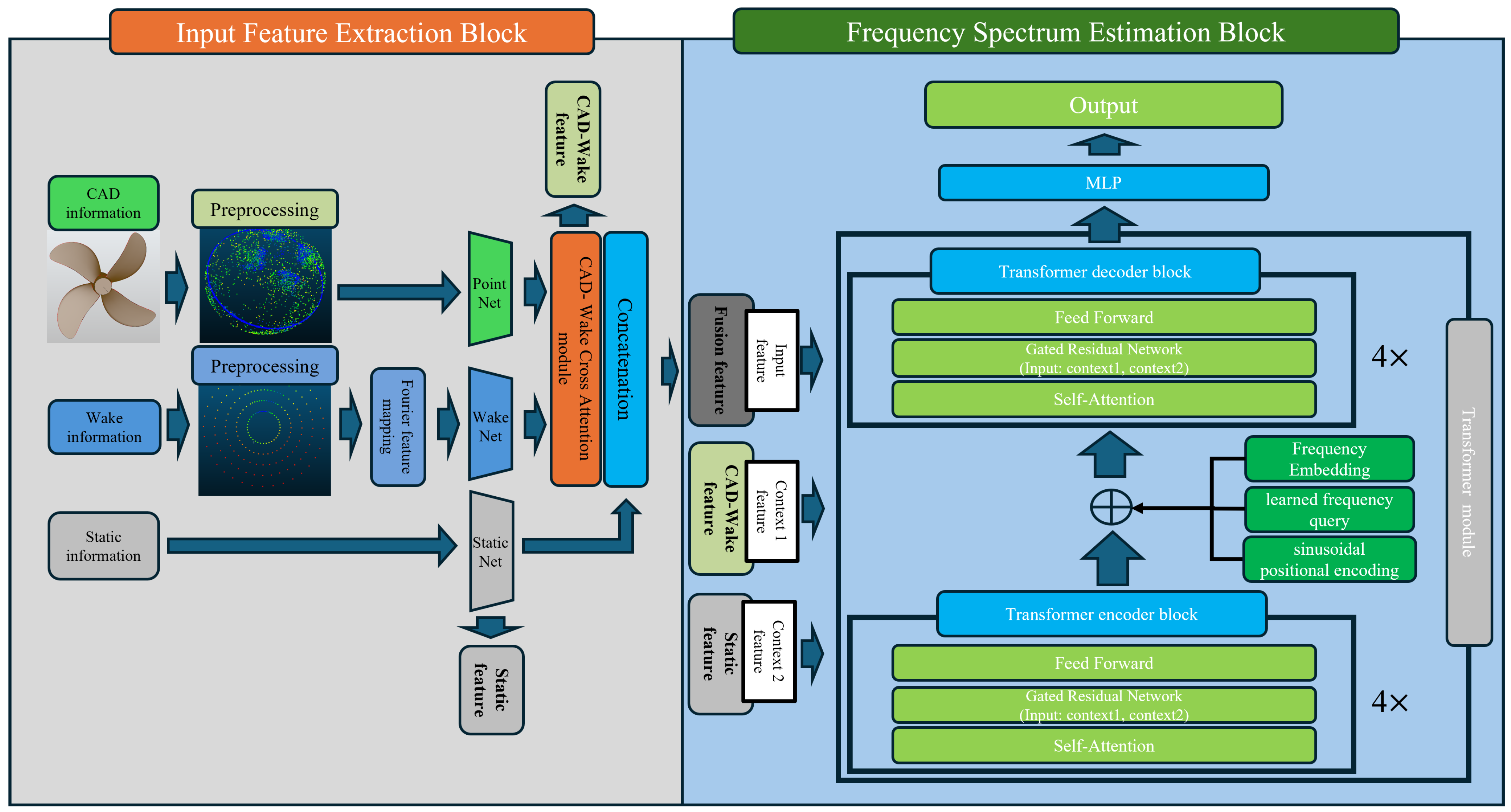
To address these limitations, this study proposes a data-driven deep learning network, MSPFS-Net, capable of estimating the fluctuating pressure frequency spectrum, as illustrated in Figure 1. The proposed model takes as inputs the propeller CAD data, principal particulars, wake distribution data, and the operating conditions of the cavitation tunnel, and predicts the frequency spectrum of pressure fluctuations acting on hull-mounted pressure sensors.

For training, the network adopts a supervised learning approach in which experimentally measured pressure signals are transformed into frequency spectra and used as the ground truth. During the testing phase, the model estimates the pressure-fluctuation frequency spectrum from only the input data.

3.2. Data Preprocessing

The proposed method first preprocesses the propeller CAD images and the wake data for each experimental case before providing them as inputs to the deep learning network. Figure 2 shows the preprocessing pipeline for the propeller CAD model. When a raw CAD model is directly fed into the network, the model may be recognized as different geometries depending on its coordinate values and phase, even if the underlying shape is identical. To prevent this issue, surface normal vectors are extracted, curvature data is computed using principal component analysis (PCA), and the result is used as network input. This preprocessing procedure is designed to isolate the geometric characteristics of the CAD model, ensuring that only intrinsic shape information is provided to the network, independent of coordinate systems or phase variations.

First, the surface of the propeller CAD model corresponding to the experimental conditions is decomposed into a triangular mesh. Next, surface points are uniformly sampled 10,000 points using a probability distribution proportional to the area of each triangle. Within each selected triangle, random points are generated according to a uniform distribution, resulting in area-unbiased surface sampling over the entire geometry. The 10,000 point cloud sampled from the CAD data is then translated so that its centroid is at the origin and scaled by the propeller diameter. Subsequently, all coordinate components are normalized to a unit range based on the maximum absolute coordinate value, thereby eliminating geometric scale effects and improving the stability of network training. Next, for each point ${\mathbf{p}}_i$ in the sampled point cloud, the k nearest neighboring points are selected based on Euclidean distance using a k-nearest neighbor (k-NN) algorithm.

$${\mathcal{N}}_i=\{{\mathbf{p}}_{i_1},\dots ,{\mathbf{p}}_{i_k}\}$$

(1)

As expressed in Equation (1), a local neighborhood ${\mathcal{N}}_i$ is constructed by selecting the k points closest to ${\mathbf{p}}_i$, where i can be considered as either the index of the sample point or the index of the local neighborhood. The mean of this neighborhood is then computed to form the covariance matrix.

$${\mathit{\mu }}_i={\displaystyle \frac{1}{k}}{\displaystyle \sum _{j=1}^k}{\mathbf{p}}_{i_j}$$

(2)

Equation (2) represents the computation of the mean of the local point set, where the mean vector ${\mathit{\mu }}_i$ is obtained by averaging the k neighboring points ${\mathbf{p}}_{i_j}$ selected for each point ${\mathbf{p}}_i$. Next, to compute the covariance matrix, each neighboring point is centered by subtracting the corresponding mean, and the variance information of the centered neighborhood is assembled into a covariance matrix. Eigenvalue decomposition is then performed on the covariance matrix to analyze the principal directions of local geometric variation. Equation (3) presents the formulation of the covariance matrix ${\mathbf{C}}_i$.

$${\mathbf{C}}_i={\displaystyle \frac{1}{k}}{\displaystyle \sum _{j=1}^k}({\mathbf{p}}_{i_j}-{\mathit{\mu }}_i){({\mathbf{p}}_{i_j}-{\mathit{\mu }}_i)}^{\mathsf{T}}$$

(3)

Subsequently, eigenvalue decomposition is performed on the computed covariance matrix, and the eigenvector corresponding to the smallest eigenvalue is defined as the surface normal vector at the given point. Using the same eigenvalue information, the local surface curvature is then calculated. Specifically, the eigenvalue decomposition of the covariance matrix yields eigenpairs that represent the magnitude of variance along each principal direction. By comparing the variance in the normal direction with that in the tangential directions, the degree to which the local surface spreads along the normal direction can be quantified. Based on this relationship, the curvature is computed as expressed in Equation (4).

$${\kappa }_i={\displaystyle \frac{{\lambda }_{i,1}}{{\lambda }_{i,1}+{\lambda }_{i,2}+{\lambda }_{i,3}}}$$

(4)

In Equation (4), ${\lambda }_{i,l}$ represents the eigenvalues of the covariance matrix derived from the k-nearest neighborhood of point ${\mathbf{p}}_i$, which quantify the variance along the corresponding principal directions.

In Figure 2, the visualization of curvature and normal vectors is generated by assigning the normal vectors as coordinate values and representing the curvature through color intensity. For network input, the normal vectors $(n_x,n_y,n_z)$ and curvature information are provided to the network without positional or scale information. This design ensures that consistent geometric information is supplied to the network solely based on the shape characteristics of the model.

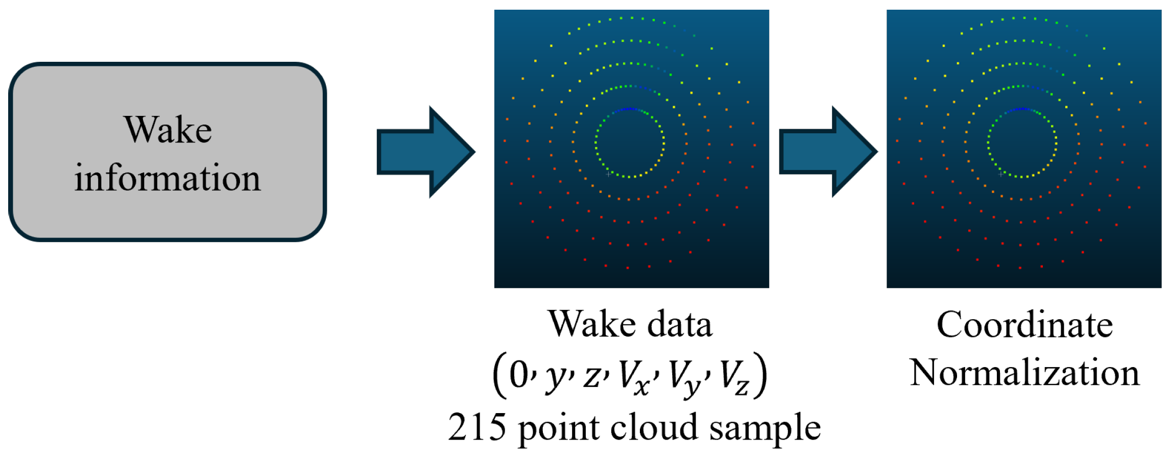
Preprocessing of wake data begins by reading the corresponding wake file, then normalizing the 215 wake points. Since the wake file contains only the y and z coordinates, the x coordinate is set to zero, and the entire coordinate set is normalized to the range $[0 ,1]$. This transformation is applied because the CAD-based shape information is provided to the network without phase information, and thus, the wake coordinates must also be converted into a scale-invariant representation. Wake data is provided to the network using six wake-related features. Figure 3 illustrates the wake preprocessing pipeline.

Next, a set of fixed parameters describing propeller specifications and operating conditions is provided to the network as static input features. These parameters include Propeller Diameter [m], Model Diameter [m], Number of Blades, Ae/Ao, Mean Pitch Ratio ($P/D_{\mathrm{mean}}$), Skew [degrees], Tip Clearance [%], Power Density, Engine Power [kW], Draught [m], Ship Speed [kts], Ship RPM resulting in a total of 12 parameters. Unlike CAD and wake data, which involve coordinate-based representations, the static parameters are used directly as raw input values without explicit preprocessing or normalization. Since these static parameters represent quantities with inherently different numerical ranges and condition-dependent variations across samples, the proposed framework was designed to process these heterogeneous physical quantities directly before latent feature transformation. To stabilize the resulting feature representations, the raw static inputs are subsequently transformed into latent features through StaticNet, which consists of linear layers, GELU activation functions, and a LayerNorm operation. This design helps mitigate potential scale imbalance effects and stabilize latent feature distributions before the features are utilized by the subsequent network modules.

3.3. Proposed Network

The proposed MSPFS-Net (Model-Test Ship Pressure Frequency Spectra Network) predicts the frequency spectrum of pressure fluctuations in a water-tunnel environment using the propeller CAD model, wake data, key propeller specifications, and experimental operating conditions as inputs. The preprocessed inputs are fed into MSPFS-Net to extract representative features, which are then transformed into a frequency spectrum consisting of 1000 bins. During training, the predicted frequency spectrum is compared with the ground-truth frequency spectrum to compute the loss. During the testing phase, MSPFS-Net estimates the frequency spectrum of pressure fluctuations solely from the input data, without requiring direct pressure-sensor measurements.

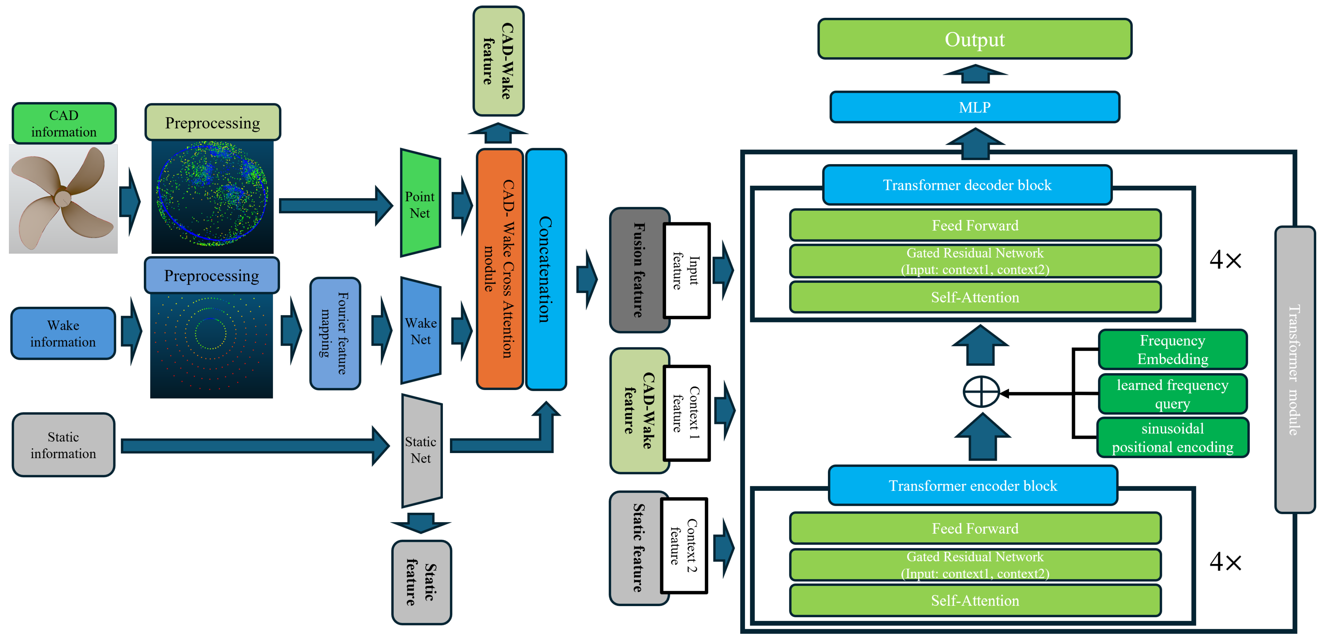
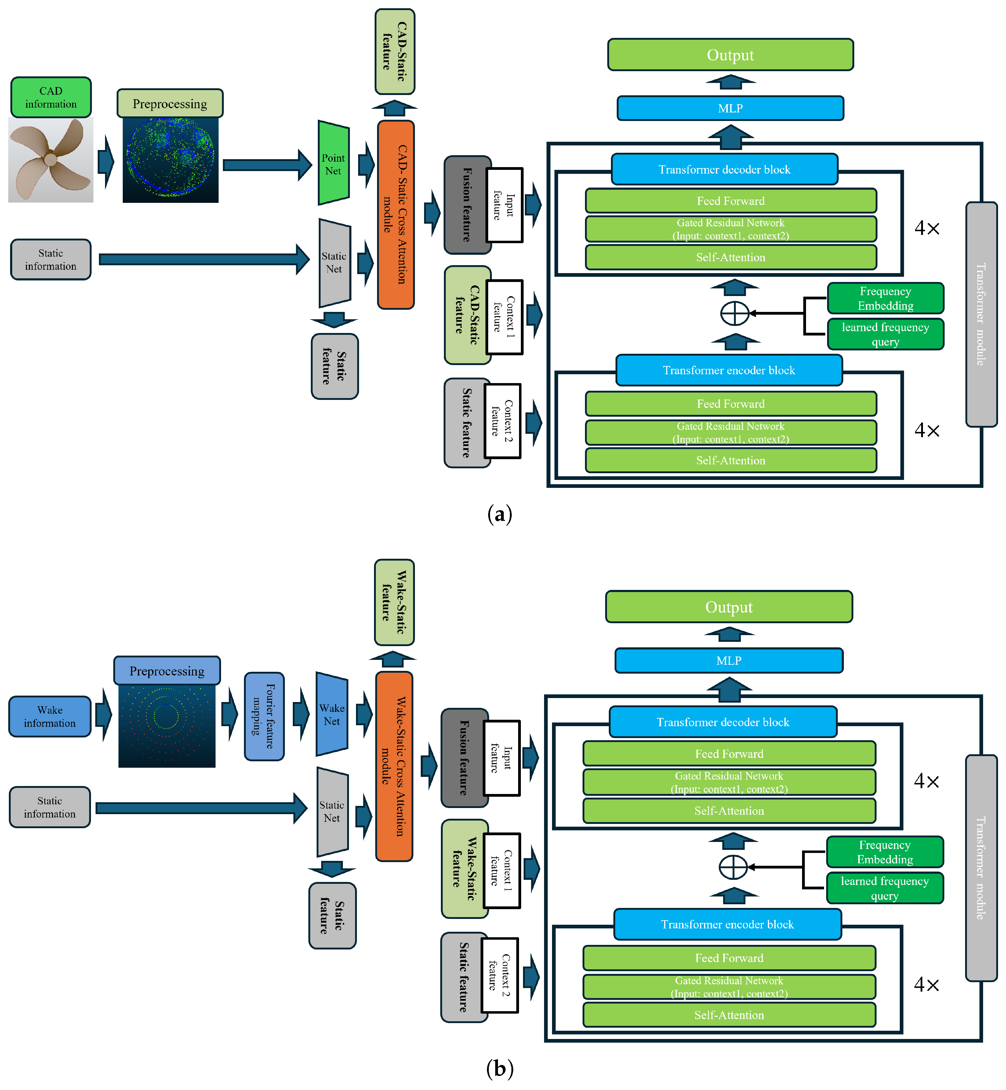
The proposed framework is composed of two main components: a feature extraction block that processes the input data, and a frequency spectrum estimation block that predicts the pressure fluctuation spectrum. Figure 4 shows the overall structure of the proposed method and its corresponding components.

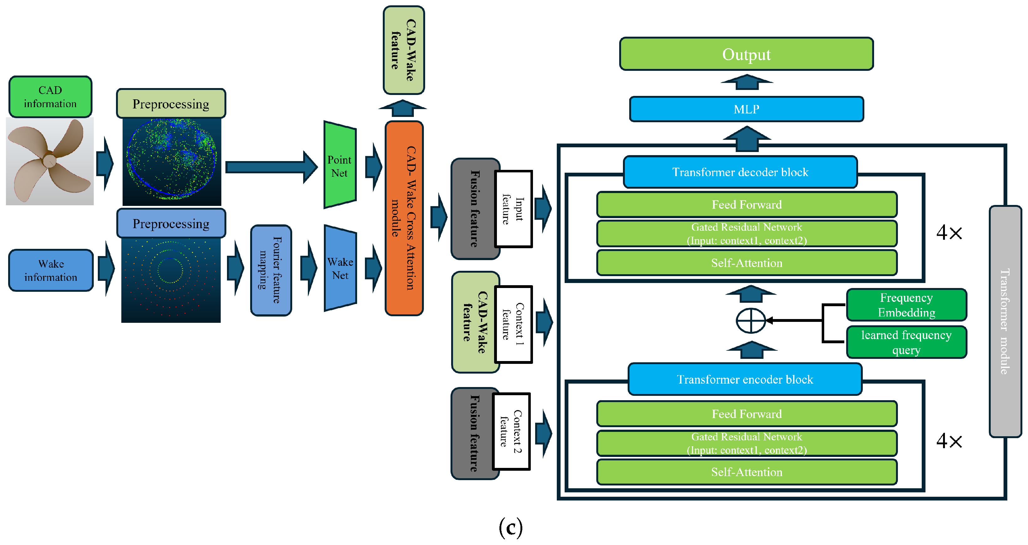
In the proposed network, the feature extraction stage consists of three components: extraction of CAD features, wake features, and static features corresponding to propeller specifications and experimental operating conditions. As illustrated in Figure 4, the extracted features are passed to the frequency spectrum estimation module in three distinct forms. First, the CAD-Wake feature is used as Context 1 in the frequency spectrum estimation module and is generated by applying an attention mechanism to the CAD and wake features. Second, the static feature, which represents fixed parameters such as propeller specifications and operating conditions, is used as Context 2 and is directly forwarded to the frequency spectrum estimation module without additional processing. Finally, the fusion feature, which is directly input to the transformer [29], is obtained by combining the CAD-Wake feature with the static feature.

3.4. Input Feature Extraction Block

3.4.1. Feature Extraction

The input feature extraction module is designed to compute correlations among input features and extract representative patterns for each input type. In this module, the input data consist of the propeller CAD model, wake data, and static parameters describing propeller specifications and experimental operating conditions. The CAD model is processed by first providing the surface normal vectors and curvature values obtained through preprocessing to a PointNet [30] architecture composed of multi-layer perceptron (MLP) layers, from which geometric features are extracted. The wake data is passed through a Fourier feature mapping [31] commonly used in NeRF [32]-based representations. Through this mapping, sinusoidal and cosine positional encodings are computed for each wake coordinate, enabling the network to represent fine-scale variations in the coordinate space better.

$$\gamma \left(x\right)={\left[sin\left(2^l\pi x\right),cos\left(2^l\pi x\right)\right]}_{l=0}^{L-1}$$

(5)

Equation (5) represents the Fourier feature mapping, where x denotes the corresponding coordinate value of the wake data. The index l denotes the frequency level, corresponding to the spatial frequencies used in NeRF-based representations. As the specified value of L increases, finer spatial details and higher-resolution structures can be represented. Lower values of l encode low-frequency information related to coarse spatial variations, while higher values of l capture high-frequency components corresponding to fine-scale details. Through this Fourier feature mapping, not only the raw spatial coordinates of the wake but also richer positional information associated with each coordinate are provided to the network, thereby enhancing the model performance. In the formulation, $\gamma (·)$ denotes the mapping that projects the input coordinates into a higher-dimensional frequency space. In the proposed method, L is set to 6.

WakeNet, which consists of multiple multi-layer perceptron (MLP) layers, processes wake data to extract representative features. Similarly, the static parameters describing propeller specifications and experimental operating conditions are encoded using StaticNet, which has an architecture analogous to that of WakeNet. The features extracted by StaticNet are subsequently used as Context 2 inputs to the Gated Residual Network [33] within the frequency spectrum estimation module, as illustrated in Figure 4.

3.4.2. CAD-Wake Cross-Attention Module

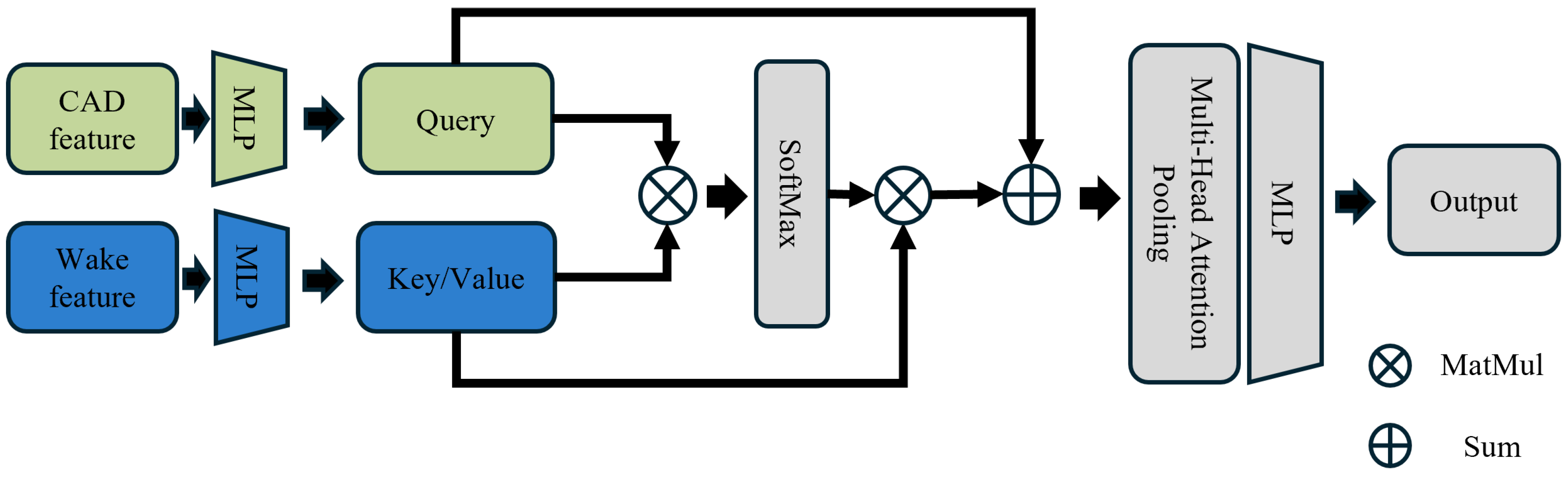
The CAD–Wake cross-attention module is designed to capture interaction cues between CAD features and wake features by conditioning CAD representations on wake data. Specifically, CAD features are projected to queries, while wake features are projected to keys and values, and cross-attention is performed to aggregate wake-aware context for each CAD point. To mitigate potential information degradation, we employ a residual connection by adding the original query features to the cross-attended outputs. The resulting wake-conditioned CAD features are then aggregated via an MLP-based attention pooling block to obtain a compact fused representation.

The CAD input is first represented as a pointwise input with shape [10,000, 4], where each point contains the normal vector components and curvature information. This input is then processed through the PointNet-based CAD feature extraction module composed of MLP layers, and the resulting latent CAD features are used to generate the query $\mathbf{Q}$. Similarly, the wake input is encoded into latent wake features, which are used to generate the key $\mathbf{K}$ and value $\mathbf{V}$.

Specifically, multi-layer perceptrons (MLPs) are applied to extract latent representations from both feature sets, generating the query $\mathbf{Q}$ from the CAD features and the key $\mathbf{K}$ and value $\mathbf{V}$ from the wake features. Cross-attention is computed using the scaled dot-product formulation:

$$\mathrm{Attention}(\mathbf{Q},\mathbf{K},\mathbf{V})=\mathrm{Softmax}\left({\displaystyle \frac{\mathbf{Q}{\mathbf{K}}^{\top }}{\sqrt{d}}}\right)\mathbf{V},$$

(6)

where d denotes the dimensionality of the key vectors. This operation enables each CAD point to selectively aggregate relevant wake data. Next To preserve CAD-specific information and mitigate potential degradation, a residual connection is applied:

$${\mathbf{F}}_{\mathrm{att}}=\mathrm{Attention}(\mathbf{Q},\mathbf{K},\mathbf{V})+\mathbf{Q}.$$

(7)

The wake-conditioned CAD features are subsequently aggregated through an MLP-based multi-head attention pooling block to obtain a compact global representation:

$${\mathbf{F}}_{\mathrm{out}}=\mathrm{Pool}\left({\mathbf{F}}_{\mathrm{att}}\right),$$

(8)

where $\mathrm{Pool}(·)$ denotes the proposed multi-head attention pooling operator. Figure 5 illustrates the architecture of the proposed CAD–Wake cross-attention module. In addition, the extracted features are used as Context 1 inputs to the Gated Residual Network in the frequency spectrum estimation module. As shown in Figure 4, the output of this module is concatenated with static features to form fused features, which are then used as inputs to the transformer module.

3.5. Frequency Spectrum Estimation Block

3.5.1. Transformer Module Encoder

The frequency spectrum estimation module transforms the features extracted from the input feature extraction module into a frequency spectrum representation. This module is a modified version of the transformer architecture [29]. Three types of input features are provided to this module: the fusion feature, which concatenates the static feature and the CAD-Wake feature, the CAD-Wake feature generated by the CAD-Wake cross-attention module, and the static feature representing fixed parameters such as experimental operating conditions.

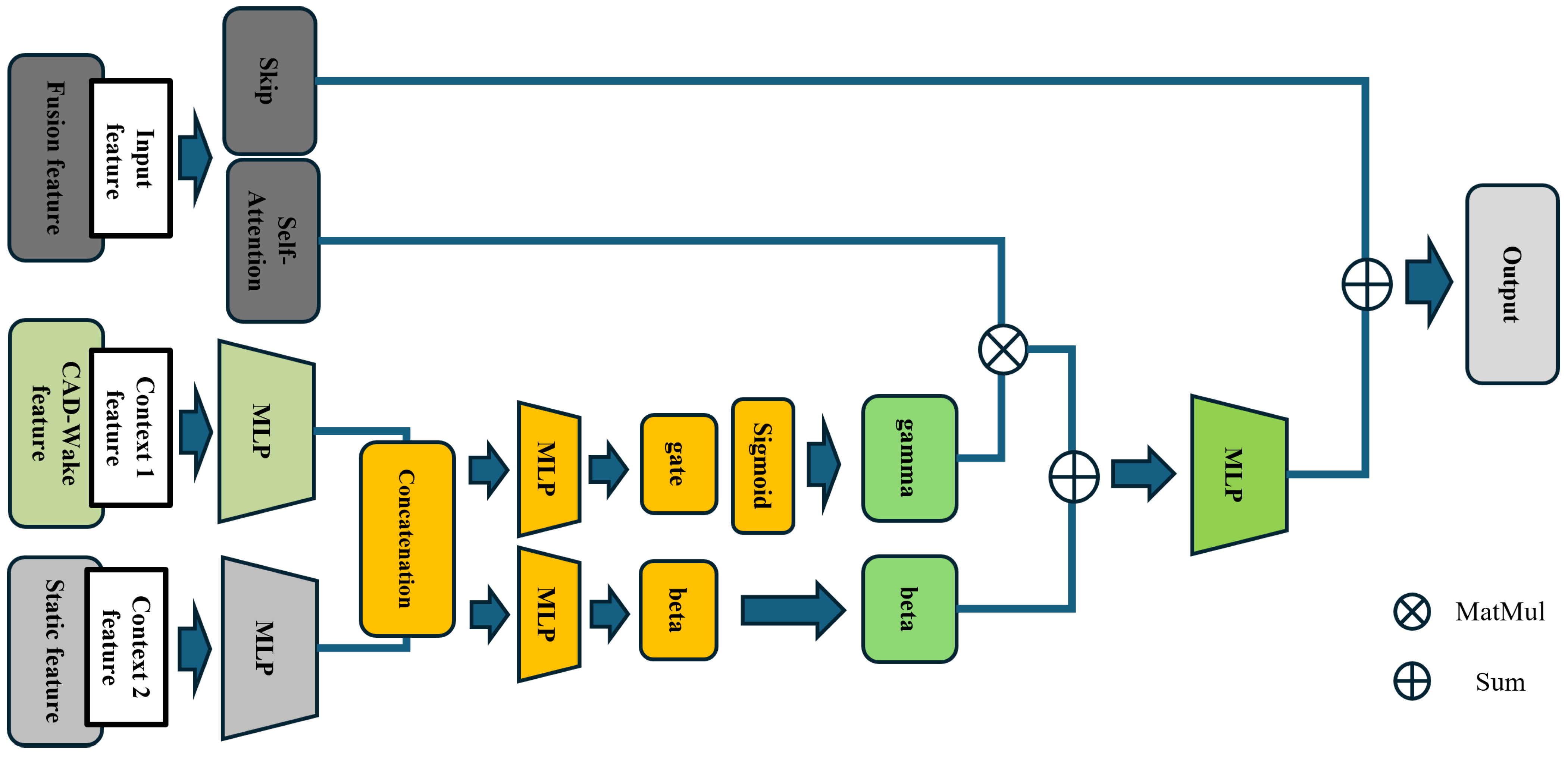
Each block of the module is composed of encoder and decoder layers. First, the encoder applies self-attention to the fusion feature to emphasize informative components and capture global dependencies. Next, a Gated Residual Network (GRN) selectively enhances meaningful information by leveraging the previously extracted CAD–Wake feature and static feature. The GRN’s gating mechanism dynamically adjusts the importance of each input feature, suppressing irrelevant signals while allowing only the most informative features to pass through. In addition, residual connections are employed to prevent information loss, thereby improving training stability and representational capacity. The architecture of the Gated Residual Network is illustrated in Figure 6.

Through the GRN, the CAD–Wake feature and the static feature are first projected separately via individual linear layers, then fused via concatenation, followed by a context fusion layer. The fused context representation is subsequently used to generate modulation parameters, which are applied to the hidden features through a Feature-wise Linear Modulation (FiLM)-like element-wise modulation mechanism. In this process, the CAD–Wake and static features act as conditioning signals that dynamically modulate the importance of the fusion feature. Subsequently, the feed-forward network refines the information aggregated by the attention mechanism. Since each position-wise vector is processed independently during forward propagation, this component is referred to as a feed-forward network. The nonlinear transformations performed in this stage further organize and refine the relational information captured by the attention mechanism.

3.5.2. Transformer Module Decoder

The decoder module serves as the output stage that directly predicts the frequency spectrum. It receives the encoder features together with frequency-related query representations for each frequency bin. These query representations are constructed using three components: (1) a learned frequency query, which is independently trainable for each frequency bin, (2) a frequency embedding that distinguishes the identity of each frequency bin, and (3) sinusoidal positional encoding, which provides structural information regarding the ordering and continuity of the frequency axis [31].

In the proposed framework, the learned frequency query and frequency embedding are mainly used to construct frequency-bin-specific representations, while the sinusoidal positional encoding acts as an auxiliary structural prior that helps preserve spectral continuity and stabilize transitions between adjacent frequency bins. In addition, the frequency embedding compensates for the potential loss of frequency-specific positional information during the encoder feature extraction process.

$$PE(\mathit{index},\mathit{i})=\left\{\begin{array}{cc}sin\left({\displaystyle \frac{\mathit{index}}{{\mathit{k}}^{\frac{\mathit{i}}{\mathrm{channel}}}}}\right),\hfill & \mathit{i}\mathrm{is}\mathrm{even},\hfill \\ cos\left({\displaystyle \frac{\mathit{index}}{{\mathit{k}}^{\frac{\mathit{i}}{\mathrm{channel}}}}}\right),\hfill & \mathit{i}\mathrm{is}\mathrm{odd}.\hfill \end{array}\right.$$

(9)

In Equation (9), index denotes the positional information corresponding to a specific frequency location, i.e., the frequency bin. The variable i represents the embedding dimension index, indicating which component of the embedding vector is being computed. In other words, index corresponds to the physical position in the input domain (frequency bin), whereas i controls the scale of the sinusoidal functions across embedding dimensions. The constant k determines how slowly the sinusoidal period increases, and is therefore related to the scaling rate of the frequency bands in the sinusoidal positional encoding. A larger value of k results in slower oscillations with longer periods, while a smaller value produces faster oscillations that can represent finer variations. Here, channel denotes the total dimensionality of the embedding vector.

In the transformer decoder, the frequency embedding and the learned frequency vector are added to the input features, and the decoder performs self-attention, the Gated Residual Network, and the feed-forward network in the same manner as the encoder. The transformer network consists of four stacked encoder–decoder blocks. Finally, the resulting features are passed through an MLP head to output the predicted frequency spectrum with the desired resolution, i.e., the specified number of frequency bins. In the proposed framework, the final output is structured as [frequency bin, sensor], where each output represents the predicted frequency spectrum of pressure fluctuations at a fixed sensor location specified in the experimental setup.

3.6. Post-Processing

The frequency spectrum predicted by the transformer exhibits excessive noise in the output. This is because the architecture does not impose structural constraints that enforce smoothness between adjacent frequency bins, and errors between neighboring bins are permitted under the formulation of the loss function. As a result, local oscillations may appear in the predicted spectrum. To mitigate this issue, the proposed method applies a post-processing step to reduce the undesired noise. Specifically, a Gaussian-based smoothing operation is performed on the predicted frequency spectrum. For this purpose, a Gaussian kernel is first defined based on the full width at half maximum (FWHM).

$$G\left(k\right)=exp\left(-{\displaystyle \frac{k^2}{2{\sigma }^2}}\right).$$

(10)

Here, $\sigma$ denotes the standard deviation computed from the FWHM, and in this study, it is set to $\sigma =1$. The variable k represents the relative kernel index with respect to the central frequency bin, and the range $k\in \{-3,\dots ,3\}$ is used in our setting. The Gaussian kernel is normalized so that its sum equals one. Subsequently, the normalized Gaussian kernel is convolved along the frequency axis to obtain the smoothed spectrum:

$${\mathrm{pred}}_{\mathrm{smooth}}\left(b\right)={\displaystyle \sum _{k=-K}^K}\mathrm{pred}(b-k)G\left(k\right),$$

(11)

Here, b denotes one of the 1000 frequency bins, and K represents the kernel half-width. $G\left(k\right)$ corresponds to the normalized Gaussian weight. In addition, to preserve the physical consistency of the spectrum, normalization was performed so that the total spectral energy remained unchanged before and after the smoothing process. Through this procedure, undesired noise was mitigated, thereby improving the accuracy of the predicted frequency spectrum.

3.7. Loss Function

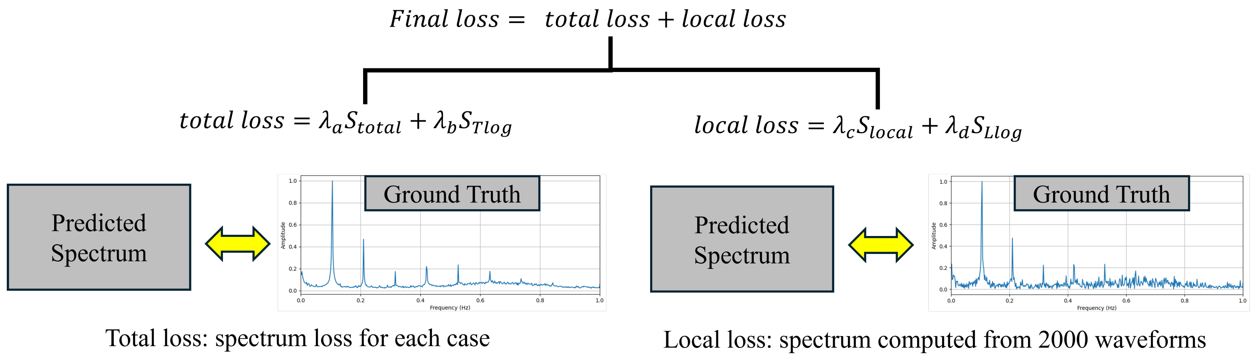
In this study, for each test condition, the pressure fluctuation frequency spectrum in the positive frequency domain is predicted with 1000 frequency bins, and the model is trained by comparing the predicted spectrum with the ground-truth spectrum. The loss function consists of two components: a total loss that evaluates the error at the overall spectrum level, and a local loss designed to reflect localized pressure fluctuation characteristics. The total loss is computed by measuring the discrepancy between a representative frequency spectrum for each test condition and the model-predicted spectrum. In contrast, the local loss is computed to capture localized pressure fluctuations under the same test conditions and to evaluate the error between partially generated frequency spectra and the corresponding model predictions. The detailed procedure for generating the ground-truth total and local frequency spectra used for training is described in Section 4.3.

Figure 7 illustrates the loss function used in the proposed method. As shown in Figure 7, the final loss is computed by summing the total loss and the local loss. Equation (12) presents the formulations of the total loss and the local loss.

$$\begin{array}{cc}\hfill \mathrm{Total}\mathrm{loss}& ={\lambda }_a{S}_{\mathrm{total}}+{\lambda }_b{S}_{T log},\hfill \\ \hfill \mathrm{Local}\mathrm{loss}& ={\lambda }_c{S}_{\mathrm{local}}+{\lambda }_d{S}_{L log}.\hfill \end{array}$$

(12)

As shown in Equation (12), the total loss consists of $S_{\mathrm{total}}$ and $S_{\mathrm{Tlog}}$, while the local loss is composed of $S_{\mathrm{local}}$ and $S_{\mathrm{Llog}}$. The terms $S_{\mathrm{Tlog}}$ and $S_{\mathrm{Llog}}$ represent the logarithmic discrepancy between the predicted and ground-truth spectra, and are defined as shown in Equation (13).

$$S_{\mathrm{Tlog}},S_{\mathrm{Llog}}={\displaystyle \frac{1}{n}}{\displaystyle \sum _{i=1}^n}{w}_i\left|y_{gt}-y_{pred}\right|$$

(13)

In Equation (13), $y_{gt}$ denotes the logarithmically transformed ground-truth frequency spectrum, while $y_{pred}$ represents the predicted frequency spectrum. The weighting factor $w_i$ in Equation (13) is defined as shown in Equation (14).

$$w_i={\left(max\left(0,Am{p}_{gtnorm,i}\right)\right)}^{\gamma }+m_w$$

(14)

The term $w_i$ is a weighting factor designed to emphasize peak components in the ground-truth frequency spectrum. In Equation (14), $\gamma$ is set to 1.5, and $m_w$ is set to 0.1. Here, $Am{p}_{gtnorm,i}$ denotes the amplitude of the ground-truth frequency spectrum at the i-th bin after normalization. The detailed definitions of $y_{gt}$ and $y_{pred}$ are given in the following equations.

$$y_{gt}=log\left(Am{p}_{gt}+\epsilon \right),y_{pred}=log\left(Am{p}_{pred}+\epsilon \right)$$

(15)

In Equation (15), $Am{p}_{gt}$ is obtained through the following normalization process, where $Am{p}_{gt}$ denotes the amplitude of the ground-truth frequency spectrum. This procedure is formulated as shown in Equation (16).

$$Am{p}_{gtnorm,i}={\displaystyle \frac{Am{p}_{gt,i}}{\frac{1}{n}{\sum }_{j=1}^{n}Am{p}_{gt,j}+\epsilon }}$$

(16)

Next, $S_{\mathrm{total}}$ and $S_{\mathrm{local}}$ are defined as weighted losses that assign higher importance to frequency bins corresponding to peak components in the ground-truth spectrum. Specifically, the weights are increased in the spectral regions corresponding to peak frequencies identified in the ground-truth frequency spectrum. The formulation of this loss is given in Equation (17).

$$S_{\mathrm{total}},S_{\mathrm{local}}={\displaystyle \frac{1}{n}}{\displaystyle \sum _{f=1}^F}{w}_{\mathrm{band},f}·w_f·{\mathrm{peakmask}}_f·\left|log(G{T}_f+\epsilon )-log(pre{d}_f+\epsilon )\right|$$

(17)

In Equation (17), $w_{\mathrm{band},f}$ denotes the bandwidth–emphasis weighting factor applied around the peak frequencies, while $w_f$ represents the weighting factor that emphasizes peak components in the overall ground-truth frequency spectrum. In addition, ${\mathrm{peakmask}}_f$ is a masking term that restricts the loss computation to frequency components exceeding a specified threshold in the spectrum. The index f corresponds to peak frequencies, and in the proposed method, the loss is computed using the top five peak frequencies identified in the ground-truth spectrum. The definition of $w_{\mathrm{band},f}$ is given in Equation (18).

$$w_{\mathrm{band},f}=\left\{\begin{array}{cc}\mathrm{factor},\hfill & {\displaystyle f\in {\displaystyle \bigcup _{k=1}^K}{\mathrm{band}}_k,}\hfill \\ 1,\hfill & \mathrm{otherwise}.\hfill \end{array}\right.$$

(18)

In Equation (18), an additional weighting factor of factor is assigned to frequency bins within the specified bandwidth regions, while the remaining bins are assigned a weight of 1.0. In this study, factor is set to 2.0. The index k denotes the bandwidth region corresponding to each peak frequency. The definition of ${\mathrm{band}}_k$ in Equation (18) is given in Equation (19).

$${\mathrm{band}}_k=\left\{f|i_k-m\le f\le i_k+m\right\}$$

(19)

Here, $i_k$ denotes the frequency-bin index corresponding to the k-th peak location in the ground-truth spectrum, and m represents the bandwidth size. In this study, m is set to 2, meaning that two neighboring bins on both the left and right sides of each peak frequency bin are included. The definition of $i_k$ is given in the following equation.

$$i_k=\arg \min \left|{\mathrm{target}}_{hz}-f_k\right|$$

(20)

In Equation (20), ${\mathrm{target}}_{hz}$ denotes the ground-truth frequency value corresponding to a peak component, while $f_k$ represents the frequency location in the predicted spectrum. The bin index closest to ${\mathrm{target}}_{hz}$ is selected and assigned as the corresponding bin position of the peak frequency. In the computation of $S_{\mathrm{total}}$ and $S_{\mathrm{local}}$, the weighting factor $w_f$ serves the same purpose as in the calculation of $S_{\mathrm{Tlog}}$ and $S_{\mathrm{Llog}}$, emphasizing peak components in the ground-truth frequency spectrum. The formulation of $w_f$ is given as follows.

$$w_f={\left(max\left(0,G{T}_{\mathrm{norm},f}\right)\right)}^{\gamma }+m_w$$

(21)

In Equation (21), $G{T}_{\mathrm{norm},f}$ denotes the normalized ground-truth frequency spectrum. The terms $S_{\mathrm{total}}$ and $S_{\mathrm{local}}$ are computed by first evaluating the logarithmic difference between the ground-truth spectrum $G{T}_f$ and the predicted spectrum $pre{d}_f$, and then multiplying the result by the corresponding weighting factors $w_{\mathrm{band},f}$ and $w_f$, as well as the masking term ${\mathrm{peakmask}}_f$. In this formulation, the loss assigns greater weight to frequency bins corresponding to the ground-truth peak locations, thereby emphasizing peak-related spectral regions during training.

4. Experiments

4.1. Experimental Setup

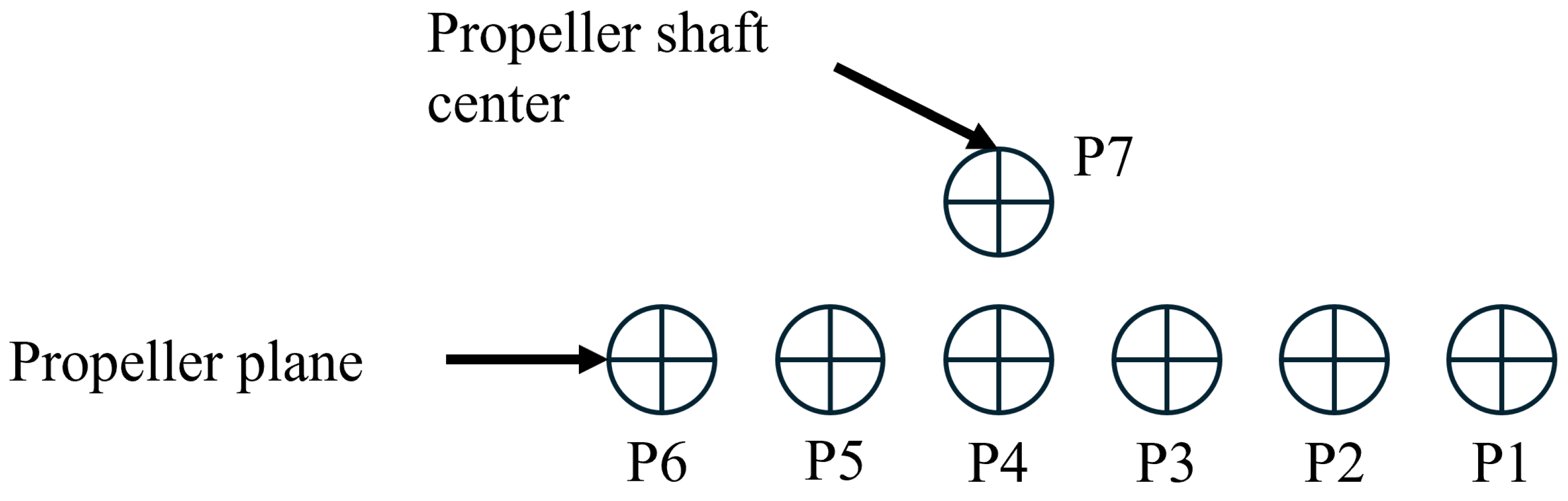
The experimental data used in this study were obtained using a cavitation tunnel configuration and measurement system consistent with that described by Shin et al. [3]. However, the locations and installation arrangement of the pressure sensors were modified in the present study, as illustrated in Figure 8. In the experiments, unsteady pressure fluctuations induced by cavitation were measured using pressure sensors fixed to the tunnel wall. Since the experimental facility and general measurement methodology have already been validated in the prior work, only a schematic illustration of the modified sensor arrangement is provided here in Figure 8.

4.2. Training Data

In the experiments, the model was trained and evaluated on 36 training sets and 10 test sets. The cases set for the training dataset are summarized in

Table 1. Training conditions used in this study.

Case	Prop. No.	Model Ship	Condition
Case_1	Prop_1	model_1	DES/BAL
Case_2	Prop_2	model_2	DES/BAL
Case_3	Prop_3	model_3	DES/BAL
Case_4	Prop_4	model_3	DES/BAL
Case_5	Prop_5	model_4	DES/BAL
Case_6	Prop_6	model_2	DES/BAL
Case_7	Prop_5	model_2	DES/BAL
Case_8	Prop_5	model_2	DES/BAL
Case_9	Prop_4	model_5	DES/BAL
Case_10	Prop_7	model_2	DES/BAL
Case_11	Prop_8	model_2	DES/BAL
Case_12	Prop_9	model_6	DES/BAL

. The model was trained on 36 distinct sets. In Table 1, Case_12 includes seven different sets of static information for each operating condition. Therefore, Cases_1 to Case_11 consist of 22 training sets, as each case includes two different operating conditions. In addition, Case_12 comprises 14 training sets, obtained by combining seven distinct sets of static information, each with two operating conditions. Consequently, the dataset consists of a total of 36 training sets.

Table 2. Test conditions used in this study.

Case	Prop. No.	Model Ship	Condition
Case_14	Prop_10	model_3	DES/BAL
Case_15	Prop_11	model_2	DES/BAL
Case_16	Prop_10	model_2	DES/BAL
Case_32	Prop_9	model_7	DES
Case_33	Prop_9	model_7	BAL
Case_34	Prop_9	model_7	DES
Case_35	Prop_9	model_7	BAL

presents the set conditions for the test dataset; a total of 10 test sets were used for evaluation. Although each of the 10 test sets represents a distinct condition, there are instances in which both the model and the propeller overlap; however, the static information remains different for each set.

4.3. Generation of Pressure Sensor Frequency Spectrum Data

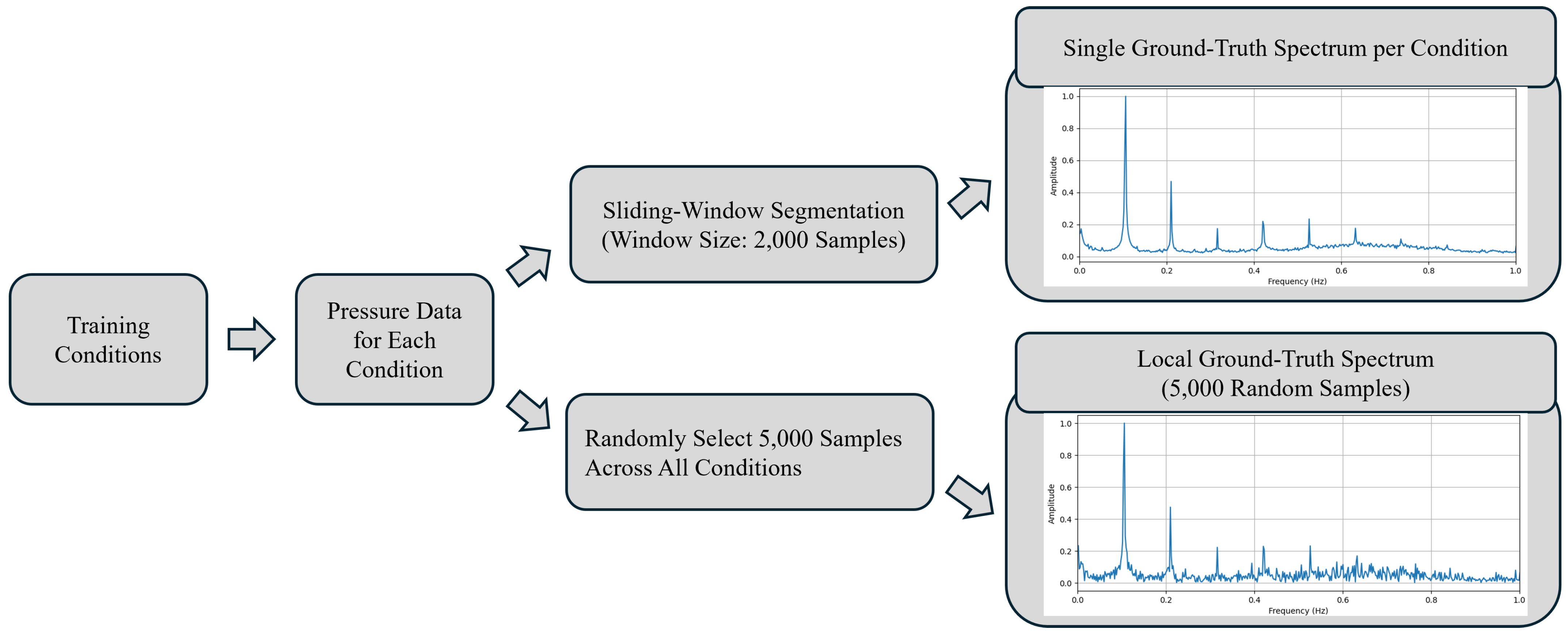
Since the proposed method is trained using a limited number of model-scale case conditions, a frequency–spectrum-based data generation strategy is applied to increase the diversity of the training data. For this purpose, two types of ground-truth frequency spectra are generated from the measured pressure fluctuation sensor signals for each training condition.

First, for each case condition c, a representative ground-truth frequency spectrum is constructed. From the total of 32,000 measured unsteady pressure sensor samples under condition c, time segments of length 2000 are extracted with an overlap of 1000 samples, resulting in 31 time segments. For each time segment, the Fast Fourier Transform (FFT) is applied, and the 1000 bins corresponding to the positive frequency domain are retained to compute the frequency spectrum. The resulting spectra are then averaged to define the representative ground-truth frequency spectrum for condition c, denoted as $s_c^{\mathrm{total}}$. In Equation (22), $\mathcal{F}$ denotes the FFT operation, and x represents the pressure sensor signal consisting of 2000 samples for each time segment.

$$s_c^{\mathrm{total}}={\displaystyle \frac{1}{31}}{\displaystyle \sum _{i=1}^{31}}\left|\mathcal{F}\left\{x_{c,i}\left(t\right)\right\}\right|$$

(22)

To further capture the characteristics of localized pressure fluctuations, additional local ground-truth frequency spectra are generated. For each test condition, a 2000-sample time segment is randomly sampled from the measured pressure fluctuation signal. The Fast Fourier Transform (FFT) is then applied to the selected segment, and the 1000 bins corresponding to the positive frequency domain are retained to compute the frequency spectrum. Through this process, multiple local spectra for condition c, denoted as $s_{c,k}^{\mathrm{local}}$, are generated as expressed in Equation (23).

$$s_{c,k}^{\mathrm{local}}=\left|\mathcal{F}\left\{x_{c,k}\left(t\right)\right\}\right|$$

(23)

In this study, a total of 5000 local spectra were generated across all training conditions and used during training. These local spectra are not entirely independent physical cases, as they are derived from the same experimentally measured pressure-fluctuation signals. Instead, the local spectrum generation process was introduced to account for local spectral variability and measurement uncertainty inherent in experimental data. Therefore, the generated local spectra serve as data augmentation and regularization, enabling the model to learn the possible spectral fluctuation characteristics that may occur under the same operating conditions. Figure 9 illustrates the training data generation procedure used in the proposed framework, including the generation process of the representative single ground-truth spectrum and the local spectra derived from measured pressure fluctuation signals.

4.4. Implementation Details

The model was trained for 20 epochs with a batch size of 4. The Adam optimizer was used with a learning rate of 0.0002. For training, 5000 samples were randomly generated across all test conditions. All experiments were conducted on a workstation equipped with an Intel Xeon W-2265 CPU and an NVIDIA RTX A5000 GPU. The frequency resolution was set to 2.4038 Hz per bin.

5. Results

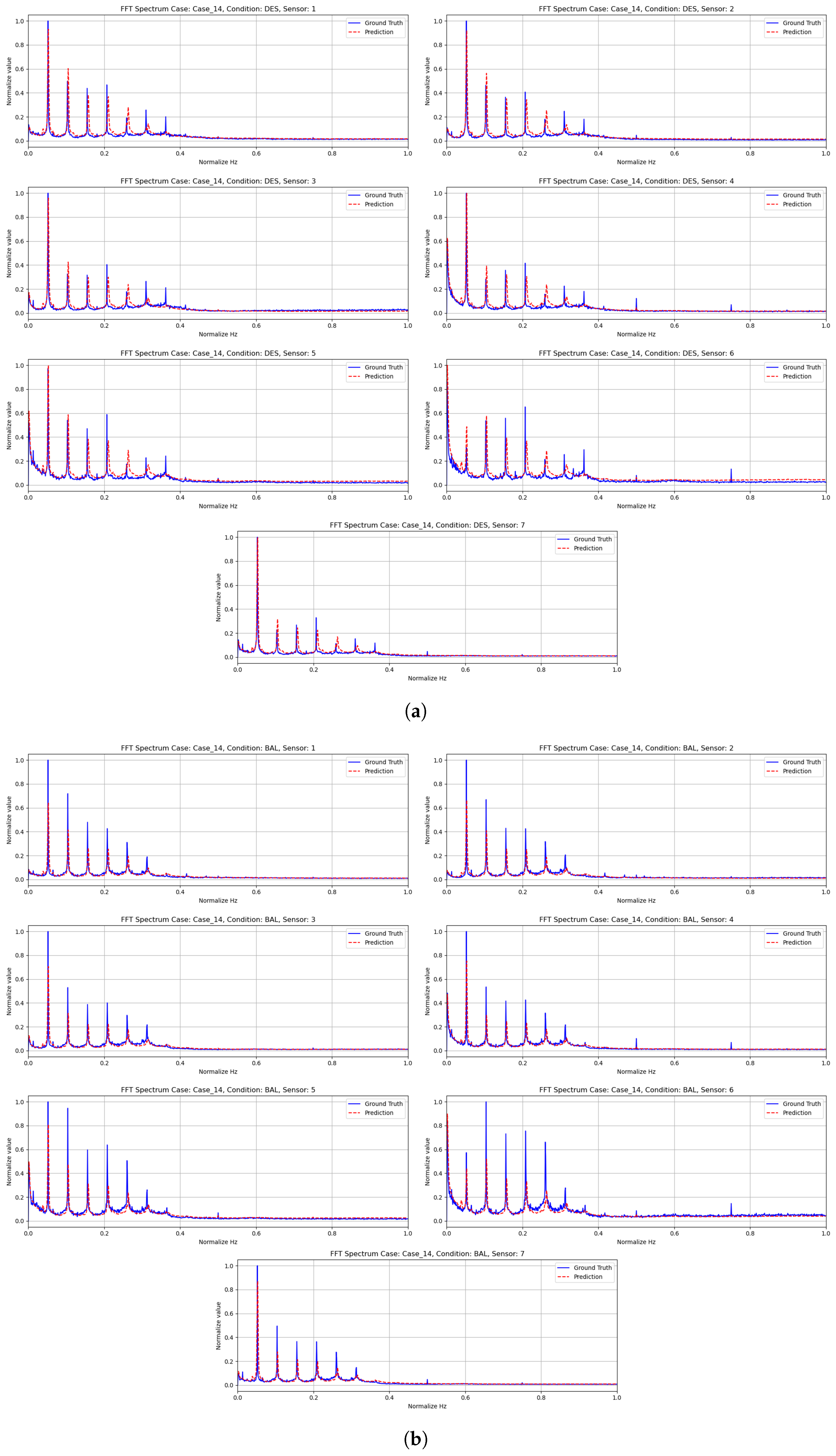
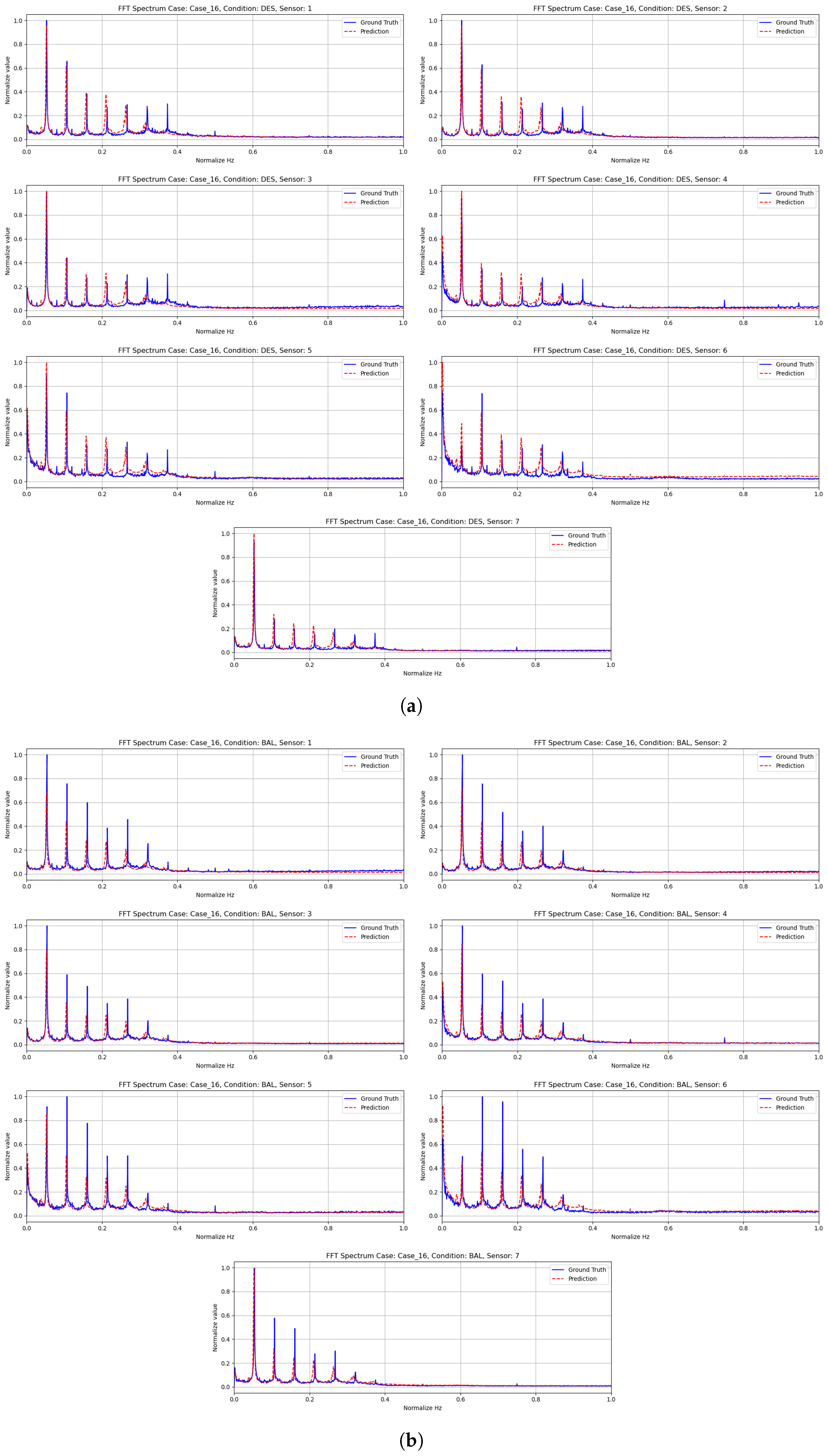
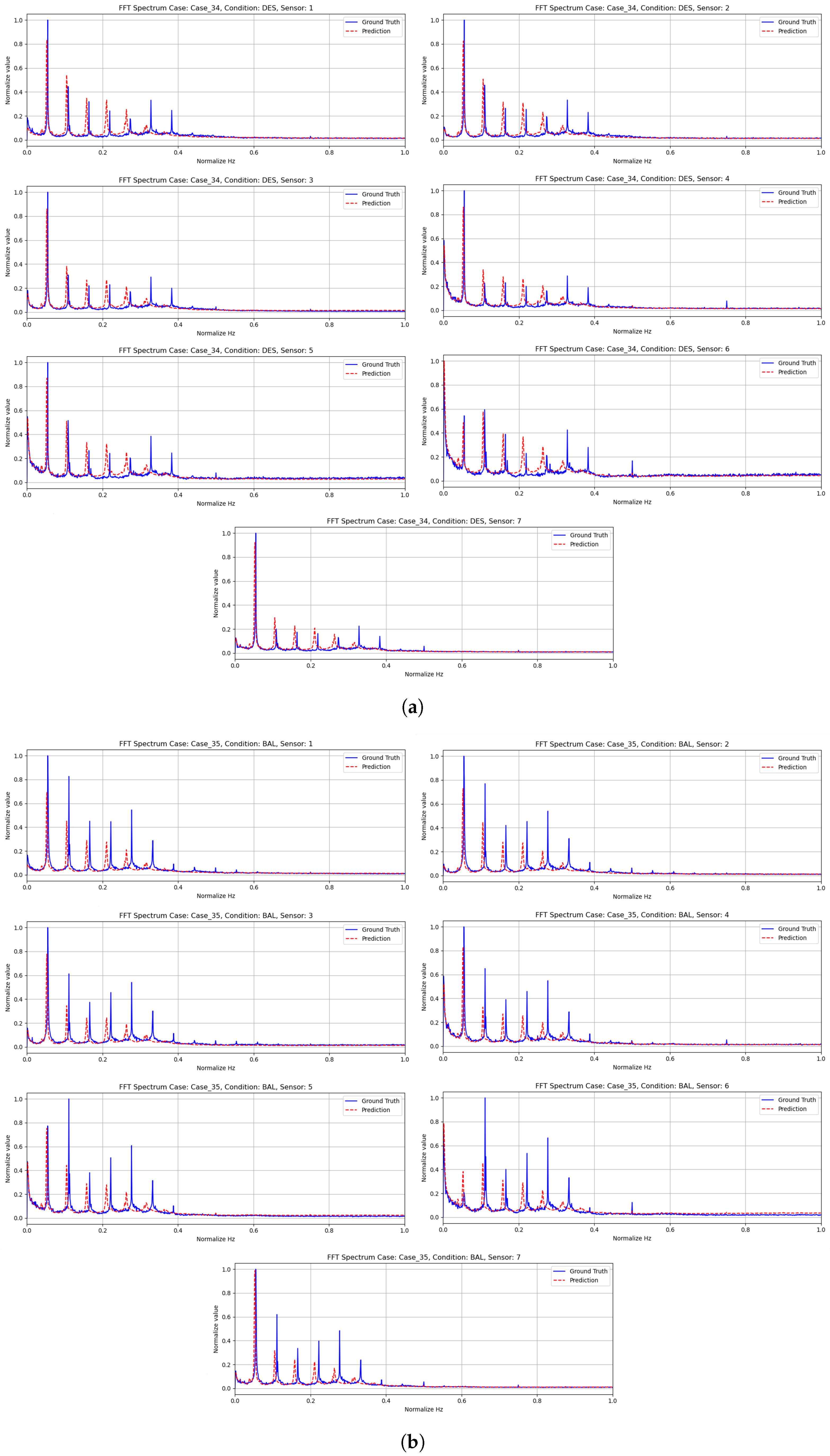
Figure 10, Figure 11 and Figure 12 present the predicted frequency spectra for each test condition. In the figures, the blue line represents the ground-truth frequency spectrum for the corresponding test condition, while the red line denotes the predicted frequency spectrum. Each figure shows the results for two operating conditions associated with each test case, as well as the results from seven pressure sensors. From left to right and top to bottom, the qualitative frequency spectrum results correspond to sensors P1 through P7.

Figure 10, Figure 11 and Figure 12 present the qualitative results of the test cases. In each figure, the ground-truth and predicted frequency spectra are compared according to the corresponding test condition and operating condition.

Table 3. Quantitative results of RMSE, correlation, and amplitude matching ratio (%).

Case [Condition]	RMSE	Correlation	Amplitude Matching Ratio (%)
			P1			P2			P3			P4
			1BF	2BF	3BF	1BF	2BF	3BF	1BF	2BF	3BF	1BF	2BF	3BF
Case_14 [DES]	0.028446	0.725357	91.29	75.16	86.93	89.00	74.21	96.09	94.56	65.70	93.47	99.76	58.01	90.05
Case_14 [BAL]	0.030699	0.702476	55.40	51.26	50.98	56.61	54.16	54.94	61.87	53.94	52.74	69.35	51.27	55.55
Case_15 [DES]	0.038993	0.547907	42.07	7.44	45.67	46.64	11.90	82.48	49.80	15.90	51.68	61.02	21.48	39.95
Case_15 [BAL]	0.045720	0.412345	26.66	3.55	27.70	30.60	5.87	68.66	33.41	6.90	82.04	43.11	8.83	99.82
Case_16 [DES]	0.027179	0.749128	94.06	93.03	96.18	94.20	92.43	80.51	98.87	99.33	84.66	92.13	85.53	77.72
Case_16 [BAL]	0.031855	0.679437	60.52	52.06	42.12	63.20	50.95	48.00	73.01	54.57	45.74	80.70	51.73	47.50
Case_32 [DES]	0.032421	0.609338	94.84	81.66	97.80	96.04	85.54	95.07	98.27	82.08	94.36	92.92	77.93	88.96
Case_33 [BAL]	0.033389	0.652155	53.84	40.29	64.35	57.29	42.35	67.48	63.66	37.57	70.32	71.31	33.03	82.45
Case_34 [DES]	0.037594	0.468045	79.63	74.72	90.53	77.14	87.06	77.98	81.75	73.80	76.79	82.95	47.28	77.17
Case_35 [BAL]	0.045752	0.396677	62.21	47.73	60.48	64.74	50.82	62.78	71.19	50.90	61.45	79.26	45.90	66.86

and

Table 4. Quantitative results of the frequency error between the ground-truth and predicted peak frequencies for the test dataset (frequency resolution: 1 bin = 2.4038 Hz). The symbol ‘×’ indicates that no predicted peak was identified within the designated bandwidth.

Case [Condition]	Frequency Difference (Hz)
	P1			P2			P3			P4
	1BF	2BF	3BF	1BF	2BF	3BF	1BF	2BF	3BF	1BF	2BF	3BF
Case_14 [DES]	2.4038	4.8076	7.2114	2.4038	4.8076	7.2114	2.4038	4.8076	7.2114	2.4038	4.8076	7.2114
Case_14 [BAL]	2.4038	2.4038	4.8076	2.4038	2.4038	2.4038	2.4038	2.4038	4.8076	2.4038	2.4038	4.8076
Case_15 [DES]	×	−21.634	14.4228	×	19.2304	14.4228	×	19.2304	14.4228	×	16.8266	14.4228
Case_15 [BAL]	×	×	12.0190	×	×	12.0190	×	×	12.0190	×	×	12.0190
Case_16 [DES]	0.000	−4.8076	−4.8076	0.000	−4.8076	−4.8076	0.000	−4.8076	−4.8076	0.000	−4.8076	−4.8076
Case_16 [BAL]	0.000	−4.8076	−7.2114	−2.4038	−4.8076	−7.2114	−2.4038	−4.8076	−7.2114	−2.4038	−4.8076	−7.2114
Case_32 [DES]	4.8076	4.8076	9.6152	4.8076	4.8076	9.6152	4.8076	4.8076	9.6152	4.8076	4.8076	9.6152
Case_33 [BAL]	2.4038	2.4038	4.8076	2.4038	2.4038	4.8076	2.4038	2.4038	4.8076	2.4038	2.4038	4.8076
Case_34 [DES]	−4.8076	−9.6152	−14.4228	−4.8076	−9.6152	−14.4228	−4.8076	−9.6152	−14.4228	−4.8076	−9.6152	−14.4228
Case_35 [BAL]	−4.8076	−14.4228	−19.2304	−4.8076	−14.4228	−19.2304	−4.8076	−14.4228	−19.2304	−4.8076	−14.4228	−19.2304

provide the quantitative evaluation results. For quantitative assessment, the proposed method evaluates the Root Mean Square Error (RMSE) and the Pearson correlation coefficient over the entire positive frequency spectrum. The average values across the seven pressure sensors are then computed. The RMSE formulation is given in Equation (24).

$$RMSE=\sqrt{\sum _{t\in M}{\left(pre{d}_t-g{t}_t\right)}^2}$$

(24)

In Equation (24), $pre{d}_t$ denotes the predicted amplitude of the frequency spectrum at the t-th bin, while $g{t}_t$ represents the corresponding ground-truth frequency spectrum amplitude. The formulation of the correlation metric is given in Equation (25).

$$corr={\displaystyle \frac{{\sum }_{t\in M}\left(pre{d}_t-pre{d}_{\mathrm{mean}}\right)\left(g{t}_t-g{t}_{\mathrm{mean}}\right)}{\sqrt{{\sum }_{t\in M}{\left(pre{d}_t-pre{d}_{\mathrm{mean}}\right)}^2}\sqrt{{\sum }_{t\in M}{\left(g{t}_t-g{t}_{\mathrm{mean}}\right)}^2}}}$$

(25)

In Equation (25), $pre{d}_{\mathrm{mean}}$ denotes the mean amplitude of the predicted frequency spectrum over all frequency bins, while $g{t}_{\mathrm{mean}}$ represents the mean amplitude of the ground-truth frequency spectrum.

In addition, the proposed method evaluates peak-level performance by selecting the peak locations from the ground-truth frequency spectrum and comparing the predicted and ground-truth values within $\pm 10$ bins around each peak (corresponding to a total bandwidth of 24.038 Hz). Here, one frequency bin corresponds to 2.4038 Hz. In Table 3 and Table 4, P1–P4 indicate the sensor indices, and 1 BF to 3 BF denote the first through third peak components in the ground-truth frequency spectrum.

In Table 3, the amplitude matching ratio represents the percentage agreement between the predicted peak amplitude and the ground-truth peak amplitude within the specified bandwidth. Table 4 reports the frequency error between the predicted and ground-truth peak frequencies within the bandwidth. The frequency difference is computed based on a resolution of 2.4038 Hz per bin. In Table 4, positive values indicate that the predicted peak frequency is higher than the ground-truth frequency, whereas negative values indicate that the predicted frequency is lower than the ground-truth value. The symbol ‘×’ in Table 4 indicates that no predicted peak was identified within the designated bandwidth, defined as ±10 bins around the ground-truth peak (i.e., a total of 20 bins). This implies that the predicted peak did not fall within the specified range and is therefore regarded as a complete prediction failure.

6. Ablation Study

In this study, an ablation analysis was conducted to quantitatively evaluate the contributions of each input component and feature extraction module in the proposed method. The full model was used as the baseline, and performance was compared by individually removing the CAD data, wake data, and static operating parameters. Quantitative evaluation was performed using RMSE and correlation coefficients as metrics, and the reported results represent the average values across all test datasets.

Figure 13 illustrates the network architectures under each ablation setting, and

Table 5. Quantitative evaluation results of the ablation study. Check mark ✓ means the corresponding components are included in the ablation study.

Model	Component			RMSE	Correlation
	CAD	Wake	Static
Ablation1 (w/o wake)	✓		✓	0.0478	0.4969
Ablation2 (w/o CAD)		✓	✓	0.0499	0.4983
Ablation3 (w/o static)	✓	✓		0.0489	0.4978
Full model (Proposed)	✓	✓	✓	0.0329	0.5654

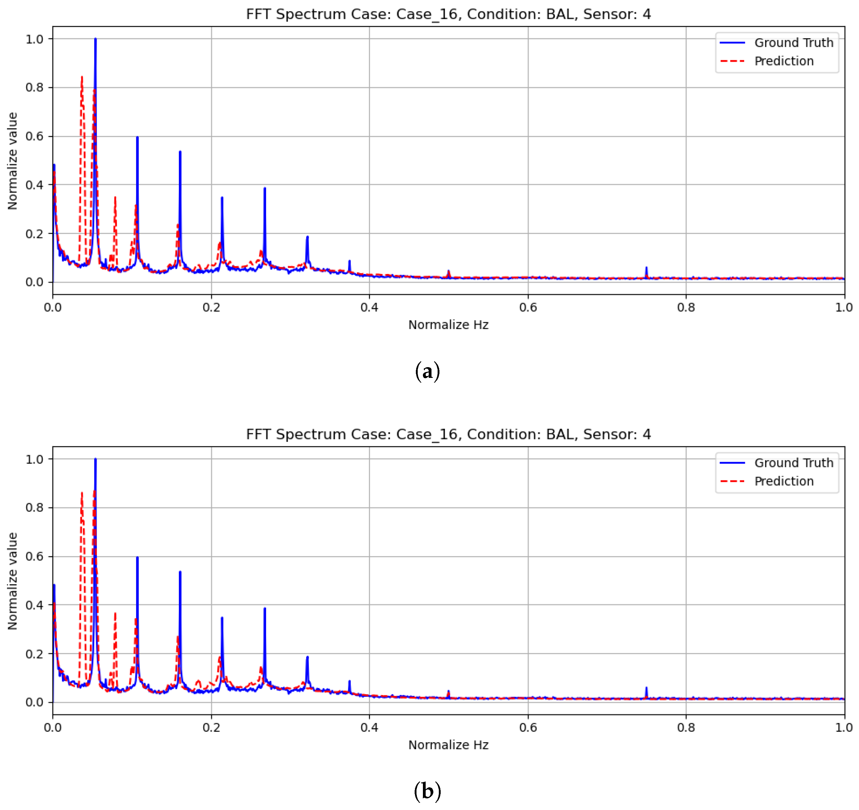
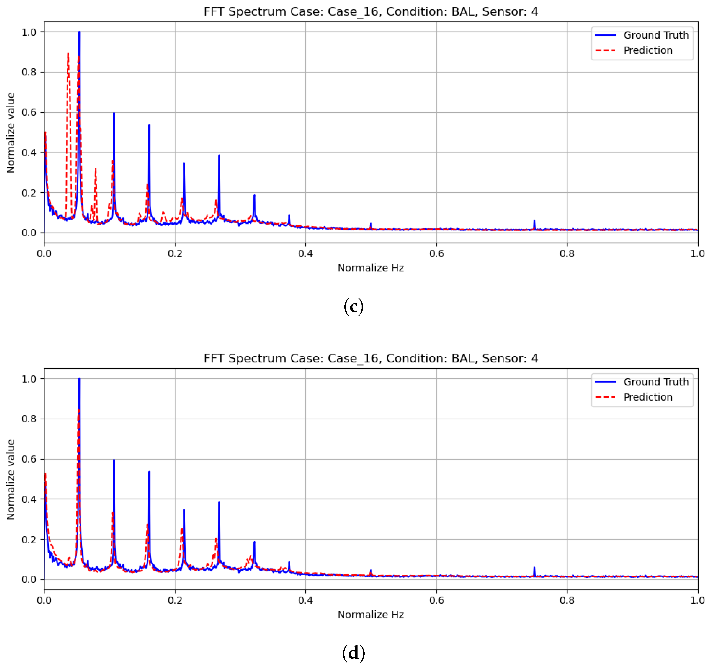
presents the corresponding quantitative evaluation results. In Table 5, CAD data is denoted as “CAD,” wake data as “Wake,” static operating parameters as “Static”. Figure 14 shows the qualitative ablation results for sensor P4 under the BAL condition of Case_16 among the seven available sensors. Sensor P4 is located near the central region between the propeller and the hull, where flow interaction effects are more pronounced. Therefore, this location is presented as a representative example for comparison.

The experimental results confirm that CAD data, wake data, and static operating parameters are all essential input components. When any one of these three types of information was excluded, the performance of fluctuating pressure frequency spectrum estimation degraded in both qualitative and quantitative aspects. This indicates that these inputs function complementarily and significantly improve estimation accuracy.

7. Conclusions

In this study, a data-driven evaluation framework for pressure fluctuations generated by a high-speed rotating marine propeller in a cavitation tunnel was developed based on model-scale experimental data. The proposed MSPFS-Net estimates the frequency spectrum of pressure fluctuations using CAD data, wake data, and static operating parameters as inputs. Unlike conventional empirical or analytical approaches, MSPFS-Net directly leverages experimental data to predict the frequency spectrum in a fully data-driven manner.

The test results demonstrate that the proposed model is capable of reproducing frequency distribution characteristics comparable to those obtained from actual experimental measurements. This indicates that, even under limited test conditions, the overall trends and dominant frequency components of the pressure fluctuation spectrum can be effectively learned. Model-scale experiments inherently involve high costs and limited test environments, which restrict the availability of diverse operating conditions. In this regard, the proposed data-driven pressure fluctuation evaluation method provides an alternative approach that effectively estimates frequency spectra using limited model-scale experimental data. However, the proposed model exhibits relatively high sensitivity to the CAD data among the input features. This dependency limits generalization performance and is partly attributable to the current network structure. Future work will focus on reducing the dependency on CAD data and improving the effective utilization of wake distribution and operating condition features within the network architecture.

In addition, direct comparisons with conventional CFD-based approaches and simpler ML-based baseline models were not included in the present study. Therefore, establishing fair and consistent benchmark settings for comparison with existing approaches remains an important topic for future research.

Furthermore, future studies will extend the framework to a wider range of operating conditions and experimental environments in order to further validate its applicability to full-scale ships. Additional experimental data and improved learning strategies will also be investigated to enhance the robustness and generalization capability of the proposed model under limited-data conditions. Although the current framework still has several limitations, the proposed approach is expected to contribute to the further development of data-driven pressure fluctuation prediction methodologies and provide useful insights for future noise and vibration prediction studies in ship hydrodynamics.

References

- Su, Y.; Kim, S.; Kinnas, S.A. Prediction of propeller-induced hull pressure fluctuations via a potential-based method: Study of the effects of different wake alignment methods and of the rudder. J. Mar. Sci. Eng. 2018, 6, 52. [Google Scholar] [CrossRef]
- Zhang, C.; Shi, Z. Empirical mode decomposition of ship hull pressure fluctuation induced by cavitating propeller. AIP Adv. 2021, 11, 085008. [Google Scholar] [CrossRef]
- Shin, Y.-J.; Kim, J.; Lee, S.; Park, D.; Kim, H. Correlation study of propeller cavity extent and pressure fluctuation for LNG feeder container ship with and without pre-swirl stator. Ocean Eng. 2024, 313, 119450. [Google Scholar] [CrossRef]
- Alves Pereira, F.; Di Felice, F.; Salvatore, F. Propeller cavitation in non-uniform flow and correlation with the near pressure field. J. Mar. Sci. Eng. 2016, 4, 70. [Google Scholar] [CrossRef]
- Li, D.-Q.; Hallander, J.; Johansson, T. Predicting underwater radiated noise of a full scale ship with model testing and numerical methods. Ocean Eng. 2018, 161, 121–135. [Google Scholar] [CrossRef]
- Lee, J.-H.; Han, J.M.; Park, H.G.; Seo, J.S. Improvements of model-test method for cavitation-induced pressure fluctuation in marine propeller. J. Hydrodyn. 2013, 25, 599–605. [Google Scholar] [CrossRef]
- Park, J.-Y.; Peric, M.; Farrall, M.; Park, C. Numerical analysis for the prediction of hull pressure fluctuation and underwater radiated noise induced by marine propeller cavitation. In Proceedings of the 10th International Symposium on Cavitation (CAV2018), Baltimore, MD, USA, 14–16 May 2018. [Google Scholar]
- Han, C.; Long, Y.; Deng, L.; Ji, B.; Long, X. Numerical analysis of propeller cavitation and pressure fluctuations around the INSEAN E779A propeller in a non-uniform wake. Ocean Eng. 2024, 312, 119310. [Google Scholar] [CrossRef]
- Viitanen, V.; Sipilä, T.; Sánchez-Caja, A.; Siikonen, T. CFD predictions of unsteady cavitation for a marine propeller in oblique inflow. Ocean Eng. 2022, 266, 112596. [Google Scholar] [CrossRef]
- Chitkeshwar, A. Revolutionizing structural engineering: Applications of machine learning for enhanced performance and safety. Arch. Comput. Methods Eng. 2024, 31, 4617–4632. [Google Scholar] [CrossRef]
- Mufti, B.; Perron, C.; Mavris, D.N. Nonlinear reduced-order modeling of compressible flow fields using deep learning and manifold learning. Phys. Fluids 2025, 37, 036130. [Google Scholar] [CrossRef]
- Liu, X.; Yang, S.; Sun, H.; Wang, Z.; Guan, X.; Gu, Y.; Wang, Y. Review of deep learning-based aerodynamic shape surrogate models and optimization for airfoils and blade profiles. Phys. Fluids 2025, 37, 041304. [Google Scholar] [CrossRef]
- As’ad, F.; Farhat, C. A mechanics-informed deep learning framework for data-driven nonlinear viscoelasticity. Comput. Methods Appl. Mech. Eng. 2023, 417, 116463. [Google Scholar] [CrossRef]
- Li, L.; Chen, Y.; Huang, L.; Hai, Q.; Tang, D.; Wang, C. Improvement of Propeller Hydrodynamic Prediction Model Based on Multitask ANN and Its Application in Optimization Design. J. Mar. Sci. Eng. 2025, 13, 183. [Google Scholar] [CrossRef]
- Zhang, J.; Mei, M.; Wang, J.; Shang, G.; Hu, X.; Yan, J.; Fang, Q. The Construction and Application of a Deep Learning-Based Primary Support Deformation Prediction Model for Large Cross-Section Tunnels. Appl. Sci. 2024, 14, 912. [Google Scholar] [CrossRef]
- Kim, S.; Kinnas, S.A. Numerical prediction of propeller-induced noise in open water and ship behind conditions. Ocean Eng. 2022, 261, 112122. [Google Scholar] [CrossRef]
- Kim, S.; Kinnas, S.A. Prediction of cavitating performance of a tip loaded propeller and its induced hull pressures. Ocean Eng. 2021, 229, 108961. [Google Scholar] [CrossRef]
- Zheng, C.; Liu, D.; Huang, H. The numerical prediction and analysis of propeller cavitation benchmark tests of YUPENG ship model. J. Mar. Sci. Eng. 2019, 7, 387. [Google Scholar] [CrossRef]
- Huang, H.-B.; Long, Y.; Ji, B. Experimental investigation of vortex generator influences on propeller cavitation and hull pressure fluctuations. J. Hydrodyn. 2020, 32, 82–92. [Google Scholar] [CrossRef]
- Wu, R.; Liu, H.; Chen, W.; Ji, S.; Cao, L.; Wu, D. Experimental investigation of propeller blade back cavitation induced pressure pulses by synchronous observation. Ocean Eng. 2024, 298, 116971. [Google Scholar] [CrossRef]
- Zhao, M.-S.; Zhao, W.-W.; Wan, D.-C. Numerical simulations of propeller cavitation flows based on OpenFOAM. J. Hydrodyn. 2020, 32, 1071–1079. [Google Scholar] [CrossRef]
- Zheng, C.-S.; Liu, K.; Liu, D.-C.; Hong, F.-W.; Zhang, Z.-R. Numerical study of the control of flow field and propeller cavitation pressure fluctuation behind the ship. J. Hydrodyn. 2025, 37, 497–504. [Google Scholar] [CrossRef]
- Zheng, C.-S.; Hong, F.-W.; Liu, D.-C.; Zhang, Z.-R. The numerical investigation of propeller cavitation benchmark tests in oblique flow. In Proceedings of the 7th International Symposium on Marine Propulsors (SMP’22), Wuxi, China, 17–21 October 2022. [Google Scholar]
- Li, L.; Chen, Y.; Xie, S.; Xiao, Y.; Fang, T.; Wang, C. Comprehensive feature-based machine learning for fast prediction of marine propeller’s open-water performance. Appl. Ocean Res. 2025, 154, 104310. [Google Scholar] [CrossRef]
- Zheng, L.; Chen, S. Data-driven prediction for the hydrodynamic behavior of propellers using a clustering ensemble learning network. Ocean Eng. 2025, 336, 121886. [Google Scholar] [CrossRef]
- Paik, K.-J.; Park, H.-G.; Seo, J. RANS simulation of cavitation and hull pressure fluctuation for marine propeller operating behind-hull condition. Int. J. Nav. Archit. Ocean Eng. 2013, 5, 502–512. [Google Scholar] [CrossRef]
- Ge, M.; Svennberg, U.; Bensow, R.E. Investigation on RANS prediction of propeller induced pressure pulses and sheet-tip cavitation interactions in behind hull condition. Ocean Eng. 2020, 209, 107503. [Google Scholar] [CrossRef]
- Bosschers, J. A semi-empirical prediction method for broadband hull-pressure fluctuations and underwater radiated noise by propeller tip vortex cavitation. J. Mar. Sci. Eng. 2018, 6, 49. [Google Scholar] [CrossRef]
- Vaswani, A.; Shazeer, N.; Parmar, N.; Uszkoreit, J.; Jones, L.; Gomez, A.N.; Kaiser, Ł.; Polosukhin, I. Attention Is All You Need. In Proceedings of the 31st International Conference on Neural Information Processing Systems (NeurIPS 2017), Long Beach, CA, USA, 4–9 December 2017; Volume 30, pp. 5998–6008. [Google Scholar]
- Qi, C.R.; Su, H.; Mo, K.; Guibas, L.J. PointNet: Deep Learning on Point Sets for 3D Classification and Segmentation. In Proceedings of the IEEE Conference on Computer Vision and Pattern Recognition (CVPR 2017), Honolulu, HI, USA, 21–26 July 2017; pp. 652–660. [Google Scholar]
- Tancik, M.; Srinivasan, P.P.; Mildenhall, B.; Fridovich-Keil, S.; Raghavan, N.; Singhal, U.; Ramamoorthi, R.; Barron, J.T.; Ng, R. Fourier Features Let Networks Learn High Frequency Functions in Low Dimensional Domains. In Proceedings of the 34th Conference on Neural Information Processing Systems (NeurIPS 2020), Vancouver, BC, Canada, 6–12 December 2020; Volume 33, pp. 7537–7547. [Google Scholar]
- Mildenhall, B.; Srinivasan, P.P.; Tancik, M.; Barron, J.T.; Ramamoorthi, R.; Ng, R. NeRF: Representing Scenes as Neural Radiance Fields for View Synthesis. In Proceedings of the European Conference on Computer Vision (ECCV 2020), Glasgow, UK, 23–28 August 2020; Volume 12346, pp. 405–421. [Google Scholar]
- Lim, B.; Arık, S.Ö.; Loeff, N.; Pfister, T. Temporal Fusion Transformers for Interpretable Multi-horizon Time Series Forecasting. Int. J. Forecast. 2021, 37, 1748–1764. [Google Scholar] [CrossRef]
Figure 1.
Overall architecture of the proposed pressure fluctuation sensor estimation network.
Figure 2.
Preprocessing pipeline for the propeller CAD model.
Figure 3.
Preprocessing pipeline for wake data.
Figure 4.
Configuration of each module in the proposed pressure fluctuation sensor estimation network.
Figure 5.
Architecture of the CAD–Wake cross-attention module.
Figure 6.
Architecture of the Gated Residual Network module.
Figure 7.
Overall structure of the proposed loss.
Figure 8.
Pressure sensor locations.
Figure 9.
Training data generation procedure for the proposed method.
Figure 10.
Qualitative frequency spectrum results for Case_14 under the corresponding operating conditions. In this figure, both the x-axis (frequency) and the y-axis (amplitude) are normalized. (a) Case: Case_14, Condition: DES. (b) Case: Case_14, Condition: BAL.
Figure 11.
Qualitative frequency spectrum results for Case_16 under the corresponding operating conditions. In this figure, both the x-axis (frequency) and the y-axis (amplitude) are normalized. (a) Case: Case_16, Condition: DES. (b) Case: Case_16, Condition: BAL.
Figure 12.
Qualitative frequency spectrum results for Case_34 and Case_35 under the corresponding operating conditions. In this figure, both the x-axis (frequency) and the y-axis (amplitude) are normalized. (a) Case: Case_34, Condition: DES. (b) Case: Case_35, Condition: BAL.
Figure 13.
Network architectures for each ablation configuration. (a) Ablation1 (w/o wake). (b) Ablation2 (w/o CAD). (c) Ablation3 (w/o static).
Figure 14.
Qualitative results for sensor P4 under each ablation configuration for Case_16 (BAL condition). In this figure, both the x-axis (frequency) and the y-axis (amplitude) are normalized. (a) Ablation1 (w/o wake). (b) Ablation2 (w/o CAD). (c) Ablation3 (w/o static). (d) Full model (Proposed).