Comparative Analysis of MADQN and QMIX Multi-Agent Reinforcement-Learning Methods for Urban Traffic Signal Control

Featured Application

The manuscript provides a comparative simulation framework for assessing traffic-signal controllers against mobility, emissions, and surrogate-safety criteria in a signalized urban grid.

Abstract

In urban areas, where car congestion is increasing daily, improving traffic-signal control is a key area of study that directly affects people’s quality of life. It is expected that such improvement will reduce environmental traffic load and increase mobility. However, the inability to determine traffic load deterministically complicates the problem. Multi-agent reinforcement-learning approaches provide a solution thanks to their adaptive learning capabilities from instantaneous data. This study evaluates the Multi-Agent Deep Q-Network (MADQN) algorithm and the QMIX value decomposition method (QMIX) in an urban traffic network with 16 signalized intersections, comparing them with Fixed-Time and Max-Pressure. Experiments were conducted under three vehicle-density levels within the same network geometry and phase-matching rules. Performance was evaluated using waiting time, travel time, speed, efficiency, carbon dioxide (CO₂) emissions, time to collision below 1 s (TTC < 1 s), and post-encroachment time below 1 s (PET < 1 s).. In all demand scenarios, both reinforcement-learning controllers achieved successful results. MADQN consistently provided lower average waiting times, whereas QMIX consistently achieved higher efficiency and, in some settings, lower CO₂ and lower cross-seed variation. No statistical superiority between MADQN and QMIX was established. Overall, the results support the value of adaptive control in this test environment and indicate trade-offs among efficiency, emissions, and proxy safety.

1. Introduction

Signalized intersections that affect the flow of urban traffic are a fundamental problem in city life that leads to traffic dependency and numerous environmental and safety outcomes, and they need to be optimally managed. The control of traffic signals at signalized intersections should be designed to minimize vehicle delays, queue length, and each vehicle’s travel time. Fixed-time traffic-signal control remains widely used worldwide because it is easy to implement. However, in real-world conditions where traffic and vehicle numbers on the roads are constantly changing, a junction managed in this manner cannot adapt to these changes due to stochastic traffic demand. Therefore, contemporary adaptive traffic-signal control is transitioning from static timing to analytical and learning-based strategies that respond to real-time traffic conditions [1,2].

Without the need for a macroscopic traffic flow model, reinforcement learning, which learns direct, adaptive, dynamic, and efficient policies by interacting with the traffic environment, has become a prominent paradigm for traffic-signal control. Reinforcement learning addresses this challenge by having an agent interact with the environment through trial and error, learning to select actions to maximize cumulative reward. Deep reinforcement learning, which emerges from combining deep neural networks with this framework, enables direct policy learning from raw traffic observations; thus, it can process high-dimensional state representations, such as queue length, waiting time, vehicle count, and phase information, without explicit model assumptions. The main advantage of this approach is that it eliminates dependence on predefined signal plans or fixed cycle lengths, allowing the controller to dynamically adapt to real-time traffic conditions [3,4].

When transitioning to multi-agent deep reinforcement learning, these advantages are transferred to the network level; while each intersection is controlled by an independent or coordinated agent, consistent policies can be developed across the network through local observations, neighboring intersection information, and centralized training mechanisms. Reinforcement and deep reinforcement learning provide not only a reactive but also a proactive, adaptable decision-making framework in traffic-signal control; this feature positions them as a promising solution family against the increasing complexity of urban traffic. It shows that deep value-based controllers can surpass weak baselines in isolated or ramp-based environments, and that collaborative multi-agent methods are becoming increasingly important when intersections are integrated at the network scale. At the same time, recent studies show that the reported performance of reinforcement-learning-based traffic-signal control depends not only on the learning architecture itself, but also on how states, rewards, and operational constraints are formulated, especially when multiple objectives must be balanced [5,6,7].

Within the scope of this study, evaluations of two multi-agent reinforcement-learning approaches were conducted across three demand levels. The results of the Fixed-Time control and Maximum-Pressure control methods were compared with those values. The experiments were conducted in an urban network comprising 16 intersections arranged in a 4 × 4 grid, with demand density scenarios at different scales. The two reinforcement learning methods were thoroughly examined in terms of their behavior within the same traffic network, the same signal-compatibility constraints, and the same demand scenarios, given their architectural structures.

Therefore, the article’s contribution is not the proposal of a new reinforcement learning algorithm, but a structured comparative study that reports mobility, emissions, and surrogate safety outcomes jointly in a multi-objective framework under systematic demand scaling. The outcomes of the study aim to provide a clear and comparative interpretation in a common simulation environment. Compared with many published studies that either focus mainly on mobility or compare learning-based controllers against limited baseline sets, the present study adds a controlled comparative evaluation in which MADQN and QMIX are examined not only against each other but also against Fixed-Time and Max-Pressure under the same network geometry, demand structure, observation basis, and phase-validity rules. In addition, the study reports mobility, CO₂, and surrogate-safety indicators jointly, evaluates robustness under systematic demand scaling, and complements descriptive comparisons with repeated-seed statistical analysis. In this sense, the manuscript contributes application-level comparative evidence on trade-offs among independent and coordinated multi-agent reinforcement learning, analytical adaptive control, and static control within a common simulation framework.

The main contributions of the paper are summarized as follows:

• The successes of a 16-intersection urban network have been evaluated against a comparative multi-objective metric, run 10 times with random seeds, and mobility, emissions, and surrogate safety indicators have been reported.
• The study evaluates the behavior of multi-agent reinforcement learning methods against each other and against other classical methods. To contextualize this, Max-Pressure was compared with Fixed-Time control as an analytical adaptive baseline.
• The multi-agent approaches MADQN and QMIX have been examined in a simulation environment across different traffic demand densities, using the same network and observation criteria, providing an application-level summary of the advantages of independent and coordinated reinforcement learning.
• The resilience of the algorithms against lighter or heavier congestion scenarios in response to systematic demand scaling has been discussed.

2. Related Work

In traffic-signal control research, the trend has shifted from fixed-duration basic cycles to continuously adaptable, learnable methods. Fixed-time scheduling determines the lengths of the components of a cycle within an intersection and the green light duration for each direction, based on stationary-demand assumptions about the number of vehicles in that intersection. It is calculated based on the practitioner’s observations and experiences. The fixed-time controller continues to serve as a reference point for comparing and evaluating other methods. The problem’s partial observability, temporal variability, and transferability characteristics make the solution complex [1,8]. Recent studies have focused on methods such as decentralized deep reinforcement learning, multi-agent reinforcement learning, graph neural networks, fuzzy-logic hybrids, and federated learning for traffic-signal control, rather than on fixed-time or actuated strategies. More recent optimization-focused studies integrate traffic prediction, graph models, and model predictive control. Thus, it offers greater responsiveness than static scheduling. However, model-based approaches have only improved generalization without accounting for stochastic periodic behaviors within the model’s framework [2].

A large body of recent work applies deep reinforcement learning to adaptive traffic-signal control. Ramp-based and isolated-intersection studies demonstrate that value-based learning can reduce delays and improve traffic progression under non-stationary traffic, with the ramp-crossing comparative study of Ouyang et al. showing that DQN improved speed, lane occupancy, and travel-time stability relative to tabular Q-learning [3]. Graves et al. demonstrated that, through a collaborative approach with a repeated-negotiation perspective among neighboring smart signals, service rates, travel times, and emissions can be improved compared to independent operation [9]. In a multi-intersection autonomous-vehicle traffic-flow setting with smart routing, Mushtaq et al. compared IA2C and MA2C with intelligent routing and concluded that coordinated actor-critic learning is better suited to multi-junction management [10]. Fang et al. proposed a fuzzy MA2C framework with a two-stream fused fuzzy deep neural network to improve robustness and generalization in traffic-signal control under uncertain and noisy communication in partially observed environments [11]. Yang et al. examined the resilience of transportation systems under accident-induced disruptions with decentralized control [12]. Han et al. proposed a method, CyLight, to achieve coordinated control with reduced communication overhead using PDQN [13]. Several influential studies provide further context. For example, PressLight linked connected reinforcement learning to max-pressure principles and demonstrated that traffic-theoretic reward design can materially improve coordination performance in signalized networks [14]. CoLight expanded network-level cooperation through learned, graph-based communication among intersections [15]. Benchmark-oriented approaches, such as RESCO, have underscored the importance of standardized tasks and realistic settings when comparing reinforcement-learning-based traffic-signal controllers [16]. Similarly, broader surveys have emphasized that progress in this area relies not only on advanced algorithms but also on transparent baselines, reproducible environments, and careful interpretation of evaluation results [8,17].

2.1. Multi-Agent Traffic-Signal Control

Isolated success for an individual intersection does not resolve the network traffic-signal control problem, because multi-intersection settings introduce non-stationarity, delayed coupling effects, and coordination requirements that do not arise in single-agent control.

Multi-agent-based reinforcement-learning (RL) methods address the coordination between junctions through mechanisms such as open communication, regional cooperation, federated aggregation, interpretable hidden state modeling, and vehicle-infrastructure coordination [18,19,20,21,22,23]. Multi-agent studies are shifting their focus from local phase selection to distributed decision-making processes. Current studies clearly demonstrate the importance of inter-agent coordination, but multi-agent studies have addressed this through different mechanisms based on network structure, state perception, or reward definitions. Examples include cooperative regional control, multi-agent DQN under high-traffic and disruption scenarios, independent deep reinforcement learning with successful experiences, and newer coordination architectures that incorporate attention or federated aggregation [18,19,20,24,25,26,27]. Taken together, these studies show that the central question is no longer whether learning-based control can outperform fixed scheduling in simple settings, but how multiple intersections should coordinate and how their performance should be evaluated at the network scale.

Hassan et al. used collaborative multi-agent reinforcement learning (MARL) to coordinate neighboring intersections within the CMDQN framework, which combines decentralized control, visual traffic features, and intersection and network rewards [28]. In this study, it has been stated that waiting times are reduced through inter-agent cooperation. Guzman et al. have shown that distributed-reinforcement learning can enhance local decision quality by using embedded representations obtained from neighboring junctions [29].

2.2. State, Action and Reward Design

The recent literature shows that the reported success of traffic-signal control based on reinforcement learning depends not only on the network architecture but also on the design of states, actions, and rewards. It has been shown that consistent state and reward design enhance convergence and interpretability [5]. State merging and trend-based reward shaping have been proposed to address sparse or delayed feedback in practical traffic control [6]. Other studies have shown that redesigning the state or reward based on additional detection information can significantly affect learned behavior. In particular, lane-specific waiting conditions and richer state inputs can alter the information base provided to the controller [30,31], while railway-aware signal control demonstrates that sensing information from railroad crossings can also influence controller behavior and traffic efficiency [32].

The design of the action space is similarly heterogeneous. Hybrid action space learning has been introduced to combine stage selection with time control [33]. Additionally, a study has shown that the quality of training can be sensitive to the selection of meta-parameters due to AutoRL-style adaptation [34]. When comparing controllers, having the same states and actions ensures a fairer comparison. Therefore, the current study has evaluated MADQN and QMIX under a common environment model, a common local observation basis, and the same stage-validity rules.

2.3. Robustness, CO₂ Emissions, Safety, and Study Positioning

Robustness and real-world applicability remain important considerations in recent traffic-signal control research. Related intelligent-transportation studies have also analyzed vulnerability to external perturbations through oscillation-based formulations, showing that damping intensity and resonance frequency can help explain why some nonlinear vehicle systems are more robust than others under sustained disturbances [35]. Multi-agent-based approaches have been examined under varying traffic loads, disruptive conditions, and stress settings designed to test robustness. Disturbance-focused studies have investigated controller behavior under heavy traffic, abnormal conditions, and robustness-enhancement settings [19,25,36]. Related studies have also explored real-time coordination through federated multi-agent optimization and vehicle–infrastructure cooperation, which further broadens the practical design space for networked traffic control [23,27].

Recent studies have also begun to treat traffic-signal control as a multi-objective task rather than a single-delay problem. In this direction, constrained and priority-aware formulations have incorporated competing public-transport requests, throughput objectives, and operational safety constraints into the control process [7]. At the same time, reward-design studies have shown that the choice of reward can materially change the trade-off among waiting time, speed, and CO₂ outcomes in reinforcement-learning-based traffic-signal control [37]. However, when evaluated from this perspective, the number of these articles remains lower than that of others.

3. Methods

This study compares two multi-agent reinforcement learning techniques, Multi-Agent Deep Q-Network (MADQN) and QMIX value-decomposition method (QMIX), with two baseline strategies, Fixed-Time control (FT) and Max-Pressure control (MP), under a common network and evaluation protocol: FT and MP serve as non-learning baselines. The objective is to regulate signal-phase decisions across a 4 × 4 urban grid to improve network mobility while enabling the broader assessment of CO₂ emissions and surrogate safety. The formal comparison results among the four controllers are presented in Section 5.

3.1. Fixed-Time Control (FT)

Fixed-Time control is used as the conventional non-learning baseline. In this approach, the existing traffic density is not considered, and the phase within a single intersection is executed in predefined durations. By changing the signals in succession according to a timetable, it allows vehicles coming from different roads to pass within specific time periods.

3.2. Max-Pressure Control (MP)

Max-Pressure control is an approach designed to optimize signal management efficiency. This is the second fundamental comparison approach used in this article. Unlike fixed-time control, which updates each intersection based on the current imbalance between upstream and downstream queues, the same phase structure used in learning-based methods also respects yellow transitions and green time constraints. In each signal phase selection, the MP algorithm selects the signal phase with the maximum pressure.

For a given intersection i, admissible green phase g, and decision time t, the phase pressure $P_i^{g\left(t\right)}$ is computed from the halting-queue counts on the lanes served by that phase. Let $I_i^g$ denote the set of incoming lanes served by phase g at intersection i, and let $O_i^g$ denote the corresponding outgoing lanes associated with those served movements. The halting-queue count on lane l at time t is denoted by $q_{l\left(t\right)}$. The phase pressure is computed as follows:

$$P_i^{g\left(t\right)}=\sum _{l\in I_i^g}{q}_{l\left(t\right)}-\sum _{m\in O_i^g}{q}_{m\left(t\right)},$$

(1)

At each decision epoch t, the controller selects the feasible green phase with the highest pressure. Let $G_i^{feas\left(t\right)}$ denote the set of feasible green phases for intersection i at time t, after applying the minimum-green and maximum-green constraints. The selected phase $g_i^{*\left(t\right)}$ is given by.

$$g_i^{*\left(t\right)}=argma{x}_{g\in G_i^{feas\left(t\right)}}{P}_i^{g\left(t\right)}$$

(2)

If multiple phases attain the same pressure value, the implementation retains the current phase to avoid unnecessary switching. If the selected phase differs from the current green phase, a yellow transition is inserted before activating the target green phase.

3.3. Multi-Agent Deep Q-Network (MADQN) Algorithm

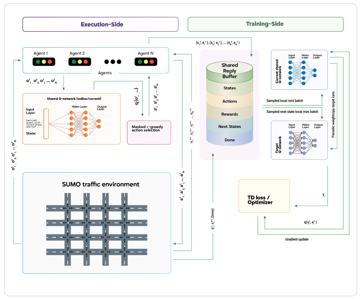
MADQN is a multi-agent, value-based, model-free, and off-policy deep reinforcement-learning algorithm. Distributed decision-making can improve rewards by leveraging neighborhood relationships and local observations. MADQN is implemented as independent Double DQN-based agents with parameter sharing. In this study, the number of agents is 16, corresponding to the 16 signalized intersections in the network. Each intersection acts as an autonomous agent that selects its own control action based on local observations, while all agents interact in the common SUMO 4 × 4 grid environment described in Section 4.1 and share a single neural action-value approximator. Parameter sharing improves sample efficiency while keeping the learning architecture compact, without eliminating decentralized decision-making. Figure 1 illustrates the architecture of signal control based on MADQN and its interaction process between the agent and the environment.

At decision step t, for agent i, the shared online network approximates the local action-value function $Q_{\theta }(O_i^t,a_i^t)$. Experiences collected from all intersections are stored in a shared replay buffer and sampled for off-policy training. Double DQN is used to reduce overestimation bias, and the network can optionally use a dueling architecture in the implemented pipeline.

$$y_i^t=r_i^t+\gamma Q_{\theta -}(o_i^{t+1},{argmax}_a{Q}_{\theta }(o_i^{t+1},a\left)\right),$$

(3)

$$L\left(\theta \right)=E\left[\right(y_i^t-Q_{\theta }(o_i^t,a_i^t){)}^2].$$

(4)

Action selection during training follows an ε-greedy policy with a linear decay schedule. A feasibility mask is applied so that the agent may only choose actions consistent with minimum-green and maximum-green rules. If a change to the green phase is selected, a yellow phase is automatically inserted before the new green phase becomes active. MADQN algorithm pseudocode is given in Algorithm 1.

Algorithm 1. Pseudocode of the MADQN Algorithm.

Require:   Environment E, 16 signalized intersections, shared online Q-network Qθ and target network Qθ−, shared replay buffer B, discount factor γ, learning rate α, ε-greedy schedule, decision interval Δt, signal constraints Output:   Trained shared Q-network weights θ; best model checkpoint   1. Initialization     Initialize θ and θ− (copy), empty replay buffer B, ε ← 1.0,     global step ← 0   2. Episode loop for episode k = 1 to 400 do     Initial local observation oᵢ0 for each intersection i ∈ {1,…,16}     Local observation: oᵢ = [vehicle count, halting count, mean speed, occupancy] × 8 lanes + one-hot(active green phase) → dim = 34   3. Decision step at each decision epoch t do     3a. Compute feasible action set Aᵢ(t) per intersection under minimum-green and maximum-green constraints     3b. Select action aᵢ with masked ε-greedy policy:       aᵢ ~ Uniform(Aᵢ(t)) with prob. ε; aᵢ ← argmaxₐ∈Aᵢ(t) Qθ(oᵢ, a) otherwise     3c. If phase change requested, insert yellow (3 s) then activate target green; else extend current green     3d. Observe oᵢᵗ+1 and local reward rᵢᵗ = w_q q̄ᵢ + w_d Δw̄ᵢ + w_tl Δτ̄ᵢ + w_epv eᵢ + w_em c̄ᵢ − w_sw zᵢ (Equation (7))     3e. Push transition (oᵢᵗ, aᵢᵗ, rᵢᵗ, oᵢᵗ+1) to B; ε ← decay(ε)   4. Learning update if |B| ≥ warm-up threshold do     Sample mini-batch of 256 transitions from B     Compute Double-DQN target: yᵢᵗ = rᵢᵗ + γ · Qθ−(oᵢᵗ+1, argmaxₐ Qθ(oᵢᵗ+1, a)) (Equations (3) and (4))     Minimize L(θ) = E[(yᵢᵗ − Qθ(oᵢᵗ, aᵢᵗ))2]; gradient clipping (norm 10.0); update θ via Adam     Every 2000 steps: synchronise target network θ− ← θ   5. Checkpoint if episode metric improves, save best model weights θ*   6. Return trained shared Q-network θ (used for decentralised evaluation)

3.4. QMIX Multi-Agent Deep Reinforcement Learning Algorithm

QMIX is an algorithm developed for multi-agent deep reinforcement learning. While preserving each agent’s local decision-making, it learns a better joint policy at the team level through collaboration. Each agent learns a separate Q network; these Q networks are then combined via a mixing network to produce the total team Q-value. QMIX is employed as the coordinated multi-agent reinforcement-learning method. As in MADQN, the number of agents is 16, corresponding to the 16 signalized intersections in the shared 4 × 4 grid environment described in Section 4.1. Each intersection still selects its action based on local observations at execution time, but training is guided by a joint action-value function that captures network-level coordination. The pseudocode of QMIX Algorithm is given in Algorithm 2.

Algorithm 2. Pseudocode of the QMIX Algorithm.

Require:   The environment E, 16 agents, shared agent utility network Qθ, mixing network fmix with hypernetworks, target counterparts Qθ− and fmix−, joint replay buffer B, discount factor γ, learning rate α, ε-greedy schedule, reward scale ρ,   running state normalizer N (mean–variance, clip ± 5), decision interval Δt, signal constraints Output:   Trained agent utility network weights θ and mixing network weights; best model checkpoint   1. Initialization     Initialize θ, θ−, fmix, fmix− (copies), empty buffer B, running normalizer N, ε ← 1.0, global step ← 0   2. Episode loop for episode k = 1 to 400 do     Reset environment; collect local observations oᵢ0 for each intersection i ∈ {1,…,16} (dim = 34 per agent)     Form global state s0 = concat(o10, …, o160) (dim = 544); normalize: ŝ0 ← N(s0)   3. Decision step at each decision epoch t do     3a. Compute feasible action set Aᵢ(t) per agent under minimum-green and maximum-green constraints     3b. Forward pass: Qθ(oᵢᵗ, ·) for all i in one batch; select aᵢ with masked ε-greedy policy (same masking rule as Algorithm 1)     3c. Apply joint action with yellow insertion and green-time feasibility (identical to Algorithm 1):       If phase change → insert yellow (3 s), then activate target green; otherwise extend current green     3d. Compute local reward ṙᵢᵗ = −queueᵢ − w_em · CO2ᵢ + w_epv · EPVᵢ − w_sw · switchᵢ;       team reward r̂ᵗ = ρ · Σᵢ ṙᵢᵗ (Equation (8))     3e. Collect next observations; form and normalize ŝᵗ+1; push joint transition (ŝᵗ, aᵗ, r̂ᵗ, ŝᵗ+1) to B; ε ← decay(ε)   4. Centralized learning update if |B| ≥ warm-up threshold do     Sample mini-batch of 256 joint transitions; reshape to per-agent local states     Compute chosen utilities: Qᵢ = Qθ(oᵢ, aᵢ); mix: Qtot = fmix(ŝ, Q1,…,Q16) (Equation (5))     Compute masked Double-Q target: yᵗ = r̂ᵗ + γ · fmix−(ŝᵗ+1, argmaxā Qθ(·, ā)) · (1 − dᵗ) (Equation (6))     Minimize Huber loss $ℒ$(Qtot, y); gradient clipping (norm 10.0); update θ and mixing weights via Adam     Every 2000 steps: synchronize θ− ← θ and fmix− ← fmix   5. Checkpoint if episode metric improves, save best agent utility and mixing network weights   6. Return trained θ (local agent policy for decentralized evaluation; mixer discarded at execution)

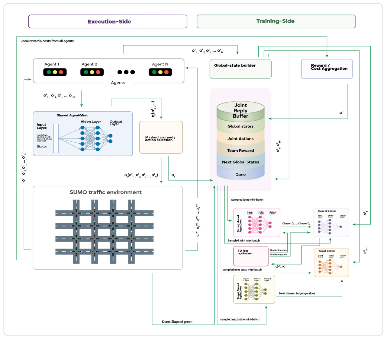
The controller uses a shared per-agent utility network that outputs local action values for each of the 16 intersections. These local utilities are combined by a mixing network to produce a joint action-value function conditioned on the global state. The global state is formed by concatenating the local observations of all intersections in a fixed junction order. The mixing network is conditioned on this global state through hypernetworks and enforces monotonicity by constraining its generated weights to be non-negative. Figure 2 illustrates the architecture of signal control based on QMIX and its interaction process between the agent and the environment.

$$Q_{tot}(s^t,a_1^t,\dots ,a_n^t)=f_{mix}(s^t,Q_1,\dots ,Q_n),$$

(5)

$$y^t={r̂}^t+\gamma Q_{tot}^{-}(s^{t+1},{ā}^{t+1})(1-d^t),$$

(6)

4. Experimental Study

This section describes the experimental setup used to evaluate the compared controllers under a common simulation framework. First, the SUMO-based network environment, observation and action settings, reward design, and parameter configuration are presented. Then, the controller performance is analyzed across the selected demand levels using mobility, CO₂, and surrogate-safety indicators.

4.1. Simulation Environment

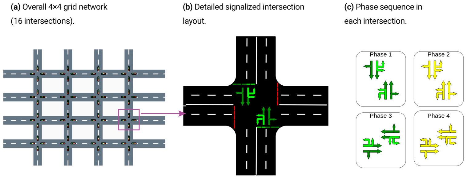
The road environment used in this study is a synthetic Simulation of Urban Mobility (SUMO) testbed rather than a real geographic location. It consists of a 4 × 4 grid network and 16 signalized intersections. To ensure that the simulation incorporates real-world conditions, the following features and constraints have been defined. The network follows a Manhattan-style grid with 200 m spacing between intersections. Vehicles in each direction can be assigned to two separate directional groups: forward-right and U-turn-left. Other directional movements have been allowed in one phase each, respectively, and each intersection is managed with 4 phases. During the transition between phases, a 3-s yellow light transition is mandatory for safety reasons. The duration of the green phases can range from 10 s to 60 s. Accordingly, the 4 × 4 SUMO urban grid constitutes the shared traffic environment for all 16 reinforcement-learning agents used in both MADQN and QMIX. The overall network environment and signal phases in intersections are given in Figure 3.

4.1.1. State Space

To make a fair comparison, both learning-based methods share a common local observation. The observation includes the number of vehicles, the number of waiting vehicles, the average speed, and the lane occupancy for the eight lanes controlled at each intersection. Additionally, the observation includes one-hot encoding indicating which phase is active.

4.1.2. Action Space Definition

For both MADQN and QMIX, each agent selects the next green phase from a discrete action set of size two. Internally, the two action indices map to the two controllable green phases available at each intersection. Yellow phases are not chosen directly by the agent; instead, they are inserted automatically whenever the selected green differs from the currently active green.

The feasible action set is further restricted by signal-timing rules. If the elapsed green time is below the minimum-green threshold, switching is disallowed. If the elapsed green time reaches the maximum-green threshold, holding the current phase is disallowed. These feasibility constraints are enforced through action masking during both training and evaluation.

4.1.3. Reward Design

Although MADQN and QMIX share the same physical environment and signal constraints, their implemented reward formulations differ. MADQN uses a richer local reward shaped by multiple operational components, whereas QMIX uses a simpler local reward that is aggregated into a team reward during centralized training. Accordingly, the RL-versus-RL findings reported later in the manuscript are interpreted as comparative evidence for the implemented controllers rather than as a fully controlled architecture-only isolation of coordination effects. This interpretation aligns with findings indicating that reward function selection significantly impacts the performance of DQN-based controllers across mobility, speed, and emissions metrics—even when the underlying algorithm and environment remain constant [37].

For MADQN, the local reward combines a normalized queue, incremental waiting time, incremental time loss, an optional CO₂ penalty, an emergency-priority bonus, and a switching penalty. More specifically, ${\bar{q}}_i$ denotes the normalized halting-queue term and penalizes local congestion; $\mathsf{\Delta }{\bar{w}}_i$denotes the increment in accumulated waiting time between two decision instants and penalizes newly incurred delay; $\mathsf{\Delta }{\bar{\tau }}_i$ denotes the increment in time loss and penalizes deterioration in traffic progression; $e_i$ denotes the emergency-priority term; ${\bar{c}}_i$ denotes the normalized CO₂-emission term; and $z_i$ is the phase-switching indicator. Except for the emergency-priority bonus, these terms act as cost components, so larger queue, delay, time loss, emissions, or unnecessary switching reduces the reward. In the implementation, these components are normalized before weighting so that no single raw quantity dominates the reward solely due to scale.

In the reported configuration, the scenario weights prioritize delay and time loss, retain a smaller queue term and switching penalty, include emergency-priority reward, and set the CO₂ weight to zero, meaning that CO₂ emissions are logged for evaluation but not directly optimized in the current MADQN weighting. Accordingly, the reported weights should be interpreted as a mobility- and operability-oriented design: delay was given the largest weight ($w_d=1.0$), time loss was kept as a secondary mobility term ($w_{tl}=0.5$), the queue term was retained as a moderate congestion regularizer ($w_q=0.2$), emergency-priority handling was explicitly rewarded ($w_{epv}=1.0$), and switching was penalized lightly ($w_{sw}=0.1$) to avoid excessive phase changes. The CO₂ term was retained in the formulation for configurability, but its reported weight was set to zero ($w_{em}=0.0$) in the present MADQN experiments. No separate TTC-based safety-penalty term is included in the implemented MADQN reward of Equation (7). Reward component weights used in MADQN are given in

Table 1. Reward component weights used in the MADQN configuration.

Weight	Description	Reward Component
1.0	Mean departure delay per vehicle (s)	delay
0.5	Mean time loss per vehicle (s)	timeLoss
0.2	Mean halting vehicle count per lane	queue
1.0	Priority bonus for emergency vehicles	epv_bonus
0.1	Phase change frequency penalty	switch_penalty
0.0	CO2 emissions per vehicle	CO2

.

$$r_i^t=w_q{q̄}_i^t+w_d{\mathsf{\Delta }w̄}_i^t+w_{tl}{\mathsf{\Delta }\tau ̄}_i^t+w_{epv}{e}_i^t+w_{em}{c̄}_i^t-w_{sw}{z}_i^t,$$

(7)

These weights govern the MADQN local reward. By contrast, the QMIX reward formulation adopts a structurally simpler form, as described below.

For QMIX, a simpler local reward is formed from the negative halting queue, an optional emissions penalty, an emergency-priority bonus, and a switching penalty. The team reward used during centralized training is obtained by summing the local rewards over all 16 agents and scaling the result by 0.01 for temporary difference updates.

$$r^t=\rho {\sum }_{i=1}^{16}{\mathsf{ṙ}}_i^t.$$

(8)

4.2. Simulation Parameter Settings

The experiments were conducted on a computer with a 2.26 GHz Xeon E7-4860 processor and 64 GB of RAM, using Python 3.8, PyTorch 2.3.1+cpu, and Traffic Control Interface (TraCI) with the SUMO 1.22 microscopic traffic simulator. Simulation parameters regarding the synthetic testbed are provided in

Table 2. Simulation environment and parameter settings.

Parameter	Setting
Network topology	Synthetic 4 × 4 urban grid with 16 signalized intersections
Road configuration	Bidirectional urban links with two lanes per edge; nominal speed 13.89 m/s
Vehicle classes	Passenger car, truck, and emergency-priority vehicle (EPV)
Simulation start/end	0 s/9200 s
Simulation step length	1 s
Decision interval	10 s
Signal constraints	Two green actions per intersection; yellow 3 s; minimum green 10 s; maximum green 60 s
Safety logging	Deterministic SSM with TTC and PET; thresholds 3 s and 2 s; range 200 m; extra time 5 s
Training demand level	scaled300
Evaluation demand levels	scaled025, scaled300, and scaled350

; it is a 4 × 4 signalized urban grid with 16 controllable intersections, each with two lanes and a nominal link speed of 13.89 m/s, featuring bidirectional urban connections. Route definitions include three vehicle classes—passenger cars, trucks, and emergency-priority vehicles (EPVs)—and class-specific dynamic parameters. In all experiments, the simulation start time, end time, and step length were fixed at 0 s, 9200 s, and 1 s, respectively. Adaptive controllers moved every 10 s, and the same signal-validity constraints were used across methods: two acceptable green actions at each intersection, a 3-s yellow transition, a 10-s minimum green, and a 60-s maximum green. The deterministic SurrogateSafety Module (SSM)was activated to record timetoCollision (TTC) and PostEncroachment Time (PET) events with thresholds of 3 s and 2 s, respectively. TTC represents the remaining time to a potential collision if two road users continue on their current trajectories and speeds, whereas PET represents the temporal gap between one road user leaving a conflict area and another entering it. Lower TTC and PET values therefore indicate more critical safety interactions. For post-surrogate-safety processing, TTC and PET events were evaluated separately in their recorded event streams. Accordingly, TTC < 1 s (%) was calculated as the percentage of logged TTC events with TTC < 1 s among logged TTC events, whereas PET < 1 s (%) was calculated as the percentage of logged PET events with PET < 1 s among logged PET events. In the present study, values below 1 s were interpreted as very severe surrogate-safety events, so lower percentages indicate safer operation. These ratios were then expressed as percentages in the reported tables and figures.

Three demand levels were considered to evaluate both nominal performance and demand robustness: scaled025, scaled300, and scaled350. These scenarios were generated by scaling a common base demand pattern, thereby preserving the same spatial origin–destination structure while varying the overall traffic loading. Consistent with the study design, the reinforcement-learning controllers were trained on the nominal-demand case (scaled300) and then evaluated across all three regimes to assess generalization under lower, matched, and higher-demand conditions. The “approximate scheduled demand (loading horizon)” reported in

Table 3. Demand-level interpretation used in the study.

Scenario	Demand Multiplier	Approximate Scheduled Demand (Loading Horizon)	Interpretation in This Study
scaled025	2.5×	≈7204 vehicles (≈7140 cars, ≈58 trucks, 6 EPVs)	Lower-demand evaluation scenario
scaled300	3.0×	≈8643 vehicles (≈8568 cars, ≈69 trucks, 6 EPVs)	Nominal scenario used for RL training and evaluation
scaled350	3.5×	≈10,083 vehicles (≈9996 cars, ≈81 trucks, 6 EPVs)	Higher-demand evaluation scenario

refers to the total number of vehicles scheduled for insertion by the predefined SUMO route/flow definitions over the 7200 s loading horizon. Accordingly, this quantity indicates how the different demand levels are instantiated in the experiments, rather than serving as a separate post hoc descriptor. The demand-scenario interpretation used in the study is presented in Table 3.

Beyond the demand multipliers themselves, the three scenarios also differ in the nominal number of vehicles scheduled for insertion over the 7200 s loading horizon. Demand is generated through time-bounded traffic flows distributed across four successive 1800 s intervals, so higher scaling increases the number of scheduled insertions while preserving the same route set and temporal structure. Thus, the approximate scheduled-demand values in Table 3 are directly tied to the route/flow inputs used in training and evaluation. Accordingly, the scenario differences are not limited to the labels 2.5×, 3.0×, and 3.5×, but also correspond to progressively larger traffic volumes throughout the episode.

Traffic demand was implemented through predefined routes and time-bounded flows rather than online rerouting. Vehicles were inserted onto fixed origin–destination paths, while lane choice at departure followed the best available lane and departures used the maximum allowed initial speed. The additional-network configuration did not introduce rerouters or other dynamic routing devices, so the reported experiments represent fixed-route demand assignment within a common network geometry.

No separate warm-up or burn-in interval was used. Traffic generation begins at the start of the episode, and the reported mobility, emissions, and safety indicators were computed over the full simulated run. Each episode ended either when the network became empty or when the simulation horizon of 9200 s was reached. The results should therefore be interpreted as full-episode performance measures rather than post-warm-up statistics.

For all controllers, throughput was calculated as the number of completed trips (i.e., arrived vehicles in the trip-level output) divided by the actual simulated duration. When a run ended before the nominal horizon due to the network becoming empty, the realized episode duration was used; otherwise, the imposed simulation end time was used.

An additional operational clarification concerns the interaction among the decision interval, yellow time, and minimum green. When a controller requests a phase change, the current green phase first transitions to its corresponding yellow phase for 3 s, after which the target green becomes active. The minimum-green and maximum-green constraints apply to the active green phase itself; that is, the minimum-green counter begins after the yellow interval has elapsed. This same switching logic is used consistently across the adaptive controllers. The remaining default settings of the SUMO microscopic traffic simulator used in the study are summarized in

Table 4. Default SUMO microscopic traffic-simulation settings used in the study.

Item	Value Used in This Study	Clarification
Car-following model	Krauss model	No explicit car-following-model override was defined in the network, route, or controller configurations.
Lane-changing model	LC2013 model	No explicit lane-changing-model override was defined.
Lateral-resolution setting	Standard lane-based simulation	Because no sub-lane extension was activated, vehicles occupied one lane laterally, and lane changes were represented without an explicit continuous lateral-motion model.
Routing assumption	Predefined routes with fixed edge sequences	Demand varied by flow intensity, not by online rerouting.
Seed usage	Training seed 42; evaluation seeds 1–10	Mean ± standard deviation values were computed from 10 seeded evaluation runs per controller and demand scenario.

.

Finally, the reported mean ± standard deviation values are based on 10 evaluation seeds for each controller and demand scenario, whereas the reinforcement-learning training runs used a separate training seed of 42. In this way, the manuscript distinguishes between the seed used to initialize the learning run and the seeds used to replicate controller evaluation under repeated SUMO executions.

The RL controller settings were read from the algorithm configuration file and then instantiated in the training scripts. To preserve partial comparability, both learning-based controllers used the same local state size, action space, discount factor, decision interval, and 400-episode training horizon. However, the QMIX implementation also used controller-specific stabilization choices, including reward scaling, running state normalization, replay warm-up, masked Double-Q target construction, Huber loss, and periodic target synchronization, and

Table 5. Reinforcement-learning model and training parameters for MADQN and QMIX.

Parameter	MADQN	QMIX
Training paradigm	Independent multi-agent Double DQN with parameter sharing	Centralized training with decentralized execution (QMIX)
Number of agents	16	16
Local state size	34	34
Global state size	Not used	544
Action size per agent	2	2
Replay capacity	200,000	500,000
Batch size	256	256
Discount factor γ	0.99	0.99
Target update interval	2000 steps	2000 steps
Exploration schedule	ε: 1.0 → 0.05 over 200,000 steps	ε: 1.0 → 0.05 over 60,000 steps
Learning rate	0.0005	0.0001
Agent hidden layers	[256, 256]	[256, 256]
Additional architecture	Dueling network; Double DQN	Mixer hidden dim = 32; hypernet layers = [64]; Double-Q + Huber; state norm; reward scale 0.01; replay warm-up 5000
Training episodes	400	400
Random seed	42	42

shows the parameters used for the RL Controllers. These implementation differences should be kept in mind when interpreting the RL-versus-RL results.

From a practical-deployability perspective, both reinforcement-learning controllers were trained for 400 episodes on the same 16-intersection grid with a 10 s decision interval. MADQN used a shared dueling Double-DQN with batch size 256 and replay capacity 200,000, whereas QMIX used centralized training with decentralized execution, a 544-dimensional global state, a mixing network with hypernetworks, and a replay capacity of 500,000. Therefore, QMIX involved higher computational overhead during training than MADQN. The retained run summaries in the present study preserve configuration details and episode-level performance results, but they do not retain exact wall-clock training duration or per-decision inference-time measurements; accordingly, the present manuscript reports relative computational overhead rather than exact runtime benchmarks.

The main assumptions and simplifications of the present study are as follows. First, the experiments were conducted on a single synthetic 4 × 4 SUMO grid rather than on a calibrated real-world corridor or city network. Second, traffic demand was implemented through predefined routes and time-bounded flows, so the study assumes fixed origin–destination paths and does not include online rerouting or adaptive route choice. Third, the signal-control formulation was deliberately simplified to two controllable green actions per intersection, with yellow phases inserted automatically and with common minimum- and maximum-green constraints across controllers. Fourth, both learning-based methods were evaluated under a common local observation design and the same network geometry, but the implemented reward and optimization settings were not identical, so the MADQN–QMIX comparison should be interpreted as a comparison of implemented controllers rather than a pure architecture-only isolation. Fifth, no separate warm-up period was used; accordingly, all reported mobility, CO₂, and surrogate-safety indicators were computed over the full simulation episode. These assumptions were adopted to preserve a controlled, reproducible comparison framework, but they also delimit the generalizability of the reported findings.

5. Results and Discussion

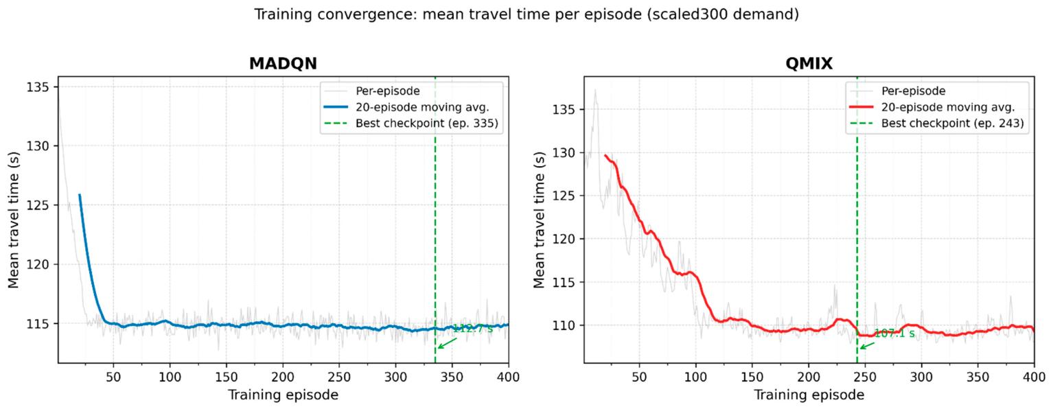
The performance of adaptive traffic-signal control frameworks is evaluated. First, the responses of the learning-based MADQN and QMIX algorithms, as well as the basic Fixed-Time and Max-Pressure methods, to three traffic-demand levels were recorded. Secondly, QMIX and the parameter-sharing-independent MADQN were run 10 times each to assess their stability under different initial conditions. Thirdly, the algorithms’ behavior in response to systematic demand changes has been examined. Finally, the analysis noted the algorithms’ behavior in response to very different multi-objective criteria, such as mobility, emissions, and surrogate safety, rather than a single KPI objective value. Since the two RL applications differ in terms of reward design and some training settings, the RL-versus-RL discussion is interpreted comparatively on an algorithmic basis. The convergence of both RL controllers over 400 training episodes is shown in Figure 4; both MADQN and QMIX approach stable performance plateaus.

Within the learning-based pair, MADQN recorded the lowest waiting time in all three demand scenarios, whereas QMIX and MADQN were nearly tied in travel time. QMIX achieved the highest throughput in every scenario, while the highest network speed was observed at scaled025 and scaled300, and was tied between MADQN and QMIX at scaled350. These results show that the transition from fixed scheduling to adaptive control yields the dominant gain, while the performance difference between independent learning and coordinated value decomposition is comparatively small and metric-dependent under the present state, action, and reward design.

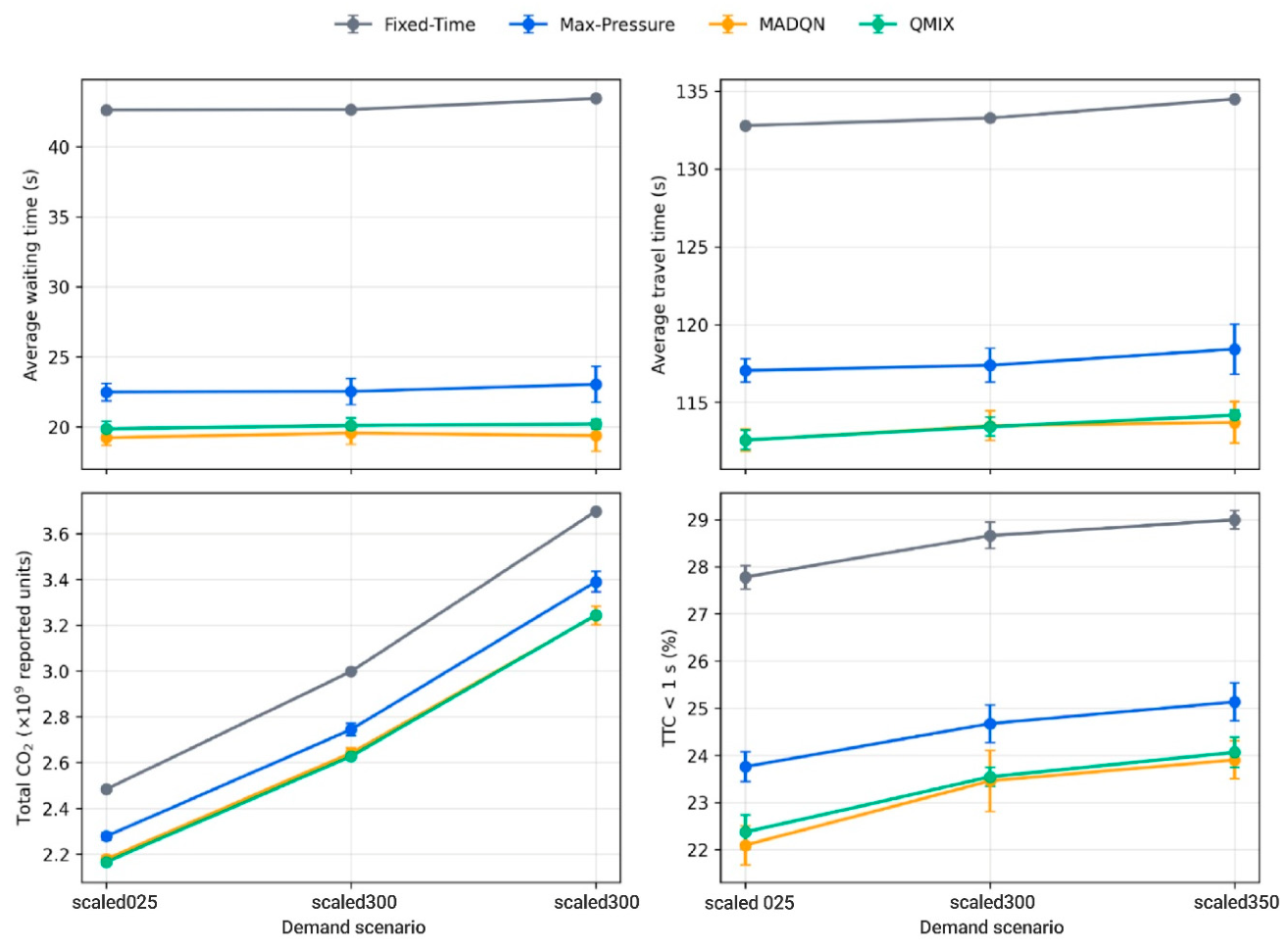
The emissions hierarchy closely mirrored the mobility results. Here, throughput (veh/h) denotes completed trips, i.e., arrived vehicles, normalized by the actual simulated duration. Total CO₂ was highest under Fixed-Time in all scenarios and lowest under RL control. Relative to Fixed-Time, Max-Pressure reduced total CO₂ by roughly 8–9%, whereas MADQN and QMIX achieved larger reductions of about 12–13% across the three scales. Safety-oriented surrogate indicators also improved substantially as we moved away from Fixed-Time. Here, TTC < 1 s (%) and PET < 1 s (%) denote the percentage of logged TTC and PET events, respectively, that fall below the 1 s severity threshold. For TTC < 1 s, Fixed-Time produced the highest severe-interaction proportions at every demand level, while the adaptive controllers reduced the ratio to approximately 22–25%. PET < 1 s showed a similar contrast between Fixed-Time and the adaptive methods, even though raw conflict totals were more mixed. Overall, within the present testbed, the baseline hierarchy can be summarized as Fixed-Time < Max-Pressure < {MADQN, QMIX}. Figure 5 shows the baseline hierarchy across demand scenarios, while

Table 6. Global summary of controller performance across demand scenarios.

Demand	Controller	Waiting Time (s)	Travel Time (s)	Speed (m/s)	Throughput (veh/h)	CO2 (×109)	TTC < 1 s (%)	PET < 1 s (%)
scaled025	Fixed-Time	42.62 ± 0.08	132.78 ± 0.10	7.80 ± 0.01	3552.09 ± 0.59	2.48 ± 0.00	27.78 ± 0.25	22.58 ± 0.64
scaled025	Max-Pressure	22.48 ± 0.63	117.05 ± 0.75	8.82 ± 0.05	3557.07 ± 5.77	2.28 ± 0.02	23.76 ± 0.32	9.49 ± 0.65
scaled025	MADQN	19.24 ± 0.55	112.57 ± 0.72	9.16 ± 0.06	3562.10 ± 3.64	2.18 ± 0.02	22.09 ± 0.41	9.23 ± 0.68
scaled025	QMIX	19.86 ± 0.54	112.58 ± 0.63	9.19 ± 0.04	3570.35 ± 4.24	2.17 ± 0.01	22.37 ± 0.36	9.10 ± 0.53
scaled300	Fixed-Time	42.65 ± 0.08	133.27 ± 0.11	7.78 ± 0.01	4256.91 ± 3.25	3.00 ± 0.00	28.66 ± 0.28	20.25 ± 1.04
scaled300	Max-Pressure	22.53 ± 0.93	117.38 ± 1.08	8.79 ± 0.08	4263.38 ± 5.60	2.74 ± 0.03	24.67 ± 0.40	8.37 ± 0.72
scaled300	MADQN	19.56 ± 0.79	113.49 ± 0.95	9.09 ± 0.07	4268.30 ± 7.96	2.64 ± 0.02	23.45 ± 0.65	8.53 ± 0.63
scaled300	QMIX	20.11 ± 0.53	113.44 ± 0.60	9.11 ± 0.04	4278.29 ± 6.90	2.63 ± 0.02	23.54 ± 0.20	8.60 ± 0.56
scaled350	Fixed-Time	43.45 ± 0.08	134.50 ± 0.11	7.70 ± 0.01	4938.11 ± 18.23	3.70 ± 0.00	29.00 ± 0.20	20.99 ± 0.48
scaled350	Max-Pressure	23.04 ± 1.29	118.41 ± 1.60	8.70 ± 0.11	4957.53 ± 7.54	3.39 ± 0.05	25.13 ± 0.40	8.00 ± 0.27
scaled350	MADQN	19.38 ± 1.13	113.71 ± 1.33	9.05 ± 0.09	4974.73 ± 7.95	3.24 ± 0.04	23.90 ± 0.40	8.30 ± 0.27
scaled350	QMIX	20.21 ± 0.33	114.17 ± 0.33	9.05 ± 0.02	4977.78 ± 11.56	3.24 ± 0.01	24.06 ± 0.32	8.50 ± 0.36

provides a global summary of controller performance across them.

5.1. Coordination Versus Independence

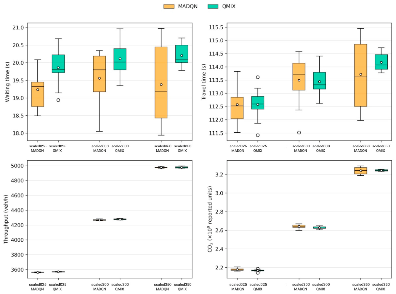
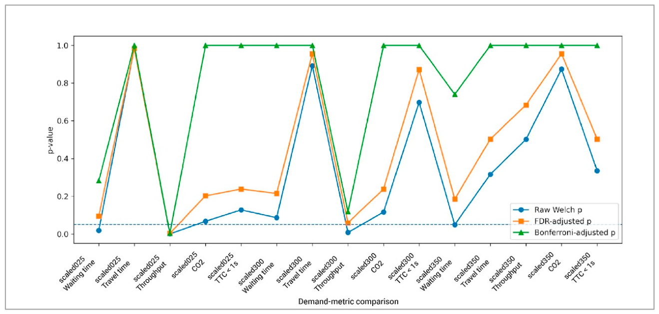
Having established that both learning-based controllers outperform the classical baselines in the studied grid, the next question is whether the coordinated QMIX implementation exhibits systematically different behavior from parameter-sharing independent MADQN. Figure 6 summarizes the descriptive per-seed distributions, whereas

Table 7. Multiplicity-corrected statistical comparison between MADQN and QMIX.

Demand	Metric	MADQN (Mean ± SD)	QMIX (Mean ± SD)	Welch p	FDR-Adjusted p	Bonferroni-Adjusted p	Hedges’ g
scaled025	Waiting time (s)	19.24 ± 0.55	19.86 ± 0.54	0.0188	0.0939	0.2816	−1.1060
scaled025	Travel time (s)	112.57 ± 0.72	112.58 ± 0.63	0.9839	0.9839	1.0000	−0.0090
scaled025	Throughput (veh/h)	3562.10 ± 3.64	3570.35 ± 4.24	0.0002	0.0030	0.0030	2.0040
scaled025	CO2 (×109)	2.18 ± 0.02	2.17 ± 0.01	0.0675	0.2024	1.0000	0.8350
scaled025	TTC < 1 s (%)	22.09 ± 0.41	22.37 ± 0.36	0.1270	0.2381	1.0000	−0.6860
scaled300	Waiting time (s)	19.56 ± 0.79	20.11 ± 0.53	0.0859	0.2148	1.0000	−0.7850
scaled300	Travel time (s)	113.49 ± 0.95	113.44 ± 0.60	0.8917	0.9553	1.0000	0.0590
scaled300	Throughput (veh/h)	4268.30 ± 7.96	4278.29 ± 6.90	0.0079	0.0589	0.1178	1.2840
scaled300	CO2 (×109)	2.64 ± 0.02	2.63 ± 0.02	0.1160	0.2381	1.0000	0.7120
scaled300	TTC < 1 s (%)	23.45 ± 0.65	23.54 ± 0.20	0.6982	0.8728	1.0000	−0.1710
scaled350	Waiting time (s)	19.38 ± 1.13	20.21 ± 0.33	0.0494	0.1851	0.7403	−0.9510
scaled350	Travel time (s)	113.71 ± 1.33	114.17 ± 0.33	0.3163	0.5032	1.0000	−0.4510
scaled350	Throughput (veh/h)	4974.73 ± 7.95	4977.78 ± 11.56	0.5017	0.6841	1.0000	0.2940
scaled350	CO2 (×109)	3.24 ± 0.04	3.24 ± 0.01	0.8740	0.9553	1.0000	−0.0700
scaled350	TTC < 1 s (%)	23.90 ± 0.40	24.06 ± 0.32	0.3355	0.5032	1.0000	−0.4240

updates the RL-versus-RL comparison by adding false-discovery-rate (FDR) and Bonferroni corrections to the 15 Welch tests reported across the three demand scenarios.

In general, MADQN yielded lower waiting time than QMIX across all three demand levels, whereas QMIX yielded higher throughput at all three demand levels and slightly lower CO₂ emissions at low and medium demand. After multiplicity correction, however, only the throughput difference at scaled025 remained statistically significant under both FDR and Bonferroni procedures. Accordingly, the MADQN–QMIX contrasts should be interpreted primarily as directional comparative tendencies rather than as a broad set of independently confirmed superiority claims.

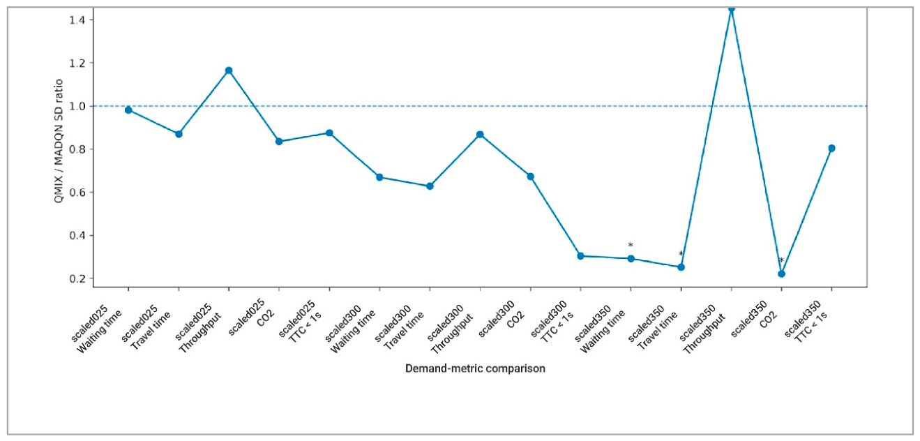
Formal equality-of-variance testing further refines this interpretation. As reported in

Table 8. Formal variance comparison between MADQN and QMIX across seeds.

Demand	Metric	MADQN SD	QMIX SD	QMIX/MADQN SD Ratio	More Stable	Brown–Forsythe p	FDR-Adjusted p
scaled025	Waiting time (s)	0.5482	0.5380	0.9813	QMIX	0.9505	0.9505
scaled025	Travel time (s)	0.7247	0.6301	0.8695	QMIX	0.6763	0.8413
scaled025	Throughput (veh/h)	3.6351	4.2358	1.1652	MADQN	0.7051	0.8413
scaled025	CO2 (×109)	0.0151	0.0126	0.8348	QMIX	0.5746	0.8413
scaled025	TTC < 1 s (%)	0.4145	0.3625	0.8746	QMIX	0.7291	0.8413
scaled300	Waiting time (s)	0.7867	0.5262	0.6688	QMIX	0.3869	0.7254
scaled300	Travel time (s)	0.9517	0.5974	0.6277	QMIX	0.3289	0.7254
scaled300	Throughput (veh/h)	7.9563	6.9019	0.8675	QMIX	0.5769	0.8413
scaled300	CO2 (×109)	0.0224	0.0151	0.6733	QMIX	0.3436	0.7254
scaled300	TTC < 1 s (%)	0.6497	0.1973	0.3037	QMIX	0.0397	0.1488
scaled350	Waiting time (s)	1.1285	0.3290	0.2916	QMIX	0.0004	0.0018
scaled350	Travel time (s)	1.3268	0.3337	0.2515	QMIX	0.0001	0.0015
scaled350	Throughput (veh/h)	7.9468	11.5567	1.4543	MADQN	0.2064	0.6191
scaled350	CO2 (×109)	0.0393	0.0087	0.2210	QMIX	0.0002	0.0015
scaled350	TTC < 1 s (%)	0.4028	0.3241	0.8045	QMIX	0.8195	0.8780

after FDR adjustment of the Brown–Forsythe procedure, significant variance differences were detected only under scaled350 for waiting time, travel time, and CO₂, with QMIX showing lower cross-seed standard deviation than MADQN in these cases. No corrected variance differences were detected for throughput or TTC < 1 s, or for scaled025 and scaled300. Thus, any QMIX stability advantage should be interpreted as selective and conditional on the high-demand setting.

Figure 6. Per-seed comparison between MADQN and QMIX. The boxplots summarize the per-seed distributions of waiting time, travel time, throughput, and total CO₂ under the three demand levels. The figure is intended as a descriptive view of the underlying distributions; formal multiplicity-corrected mean comparisons and variance tests are reported separately in Table 7 and Figure 7 and Figure 8.

Figure 6. Per-seed comparison between MADQN and QMIX. The boxplots summarize the per-seed distributions of waiting time, travel time, throughput, and total CO₂ under the three demand levels. The figure is intended as a descriptive view of the underlying distributions; formal multiplicity-corrected mean comparisons and variance tests are reported separately in Table 7 and Figure 7 and Figure 8.

Figure 7. Cross-seed standard-deviation ratios for QMIX relative to MADQN. The figure reports the ratio of QMIX standard deviation to MADQN standard deviation for each demand–metric combination. Ratios below 1.0 indicate lower variability for QMIX. Asterisks denote comparisons that remain significant after FDR adjustment of the Brown–Forsythe variance test.

Figure 7. Cross-seed standard-deviation ratios for QMIX relative to MADQN. The figure reports the ratio of QMIX standard deviation to MADQN standard deviation for each demand–metric combination. Ratios below 1.0 indicate lower variability for QMIX. Asterisks denote comparisons that remain significant after FDR adjustment of the Brown–Forsythe variance test.

Figure 8. Multiplicity-adjusted MADQN–QMIX Welch comparisons. The figure reports raw, false-discovery-rate (FDR)-adjusted, and Bonferroni-adjusted p-values for the 15 MADQN–QMIX comparisons. The dashed horizontal line indicates the conventional p = 0.05 significance threshold; points below this line are statistically significant at the 5% level. After multiplicity correction, only the throughput difference at scaled025 remains statistically significant.

Figure 8. Multiplicity-adjusted MADQN–QMIX Welch comparisons. The figure reports raw, false-discovery-rate (FDR)-adjusted, and Bonferroni-adjusted p-values for the 15 MADQN–QMIX comparisons. The dashed horizontal line indicates the conventional p = 0.05 significance threshold; points below this line are statistically significant at the 5% level. After multiplicity correction, only the throughput difference at scaled025 remains statistically significant.

5.2. Robustness Across Demand Shifts

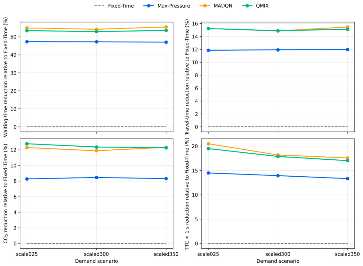
Figure 9 shows no rank reversal across the three demand levels: Fixed-Time remained the weakest controller, Max-Pressure remained a strong intermediate baseline, and MADQN/QMIX consistently delivered the best overall mobility and environmental performance. This stable ranking is consistent with useful generalization across the tested demand shifts, although this evidence remains bound to the present simulation setting.

The magnitude of the RL advantage also remained stable as demand increased from scaled025 to scaled350. For average waiting time, Max-Pressure reduced delay by about 47% relative to Fixed-Time at all three scales, MADQN by about 54–55%, and QMIX by about 53%. Travel-time and CO₂ reductions showed similar patterns of stability. The severe-interaction ratio TTC < 1 s increased with demand for all controllers, as expected under denser traffic, but the relative advantage over Fixed-Time was preserved across the demand range.

When robustness is examined through performance drift across scales, the RL controllers again appear favorable. From scaled025 to scaled350, average waiting time increased by only 0.75% for MADQN and 1.73% for QMIX, compared with 1.93% for Fixed-Time and 2.49% for Max-Pressure. These results suggest that the learned controllers degraded gracefully under rising demand within the studied grid, with MADQN showing the smallest drift in mean delay and QMIX preserving its network-level throughput advantage.

Although the present results indicate stable controller ranking under systematic demand scaling in the studied 4 × 4 grid, this evidence should not be interpreted as direct proof of the same behavior under all network forms or disturbance conditions. In an arterial network, where progression along a dominant direction and signal coordination along a corridor become more important, the relative behavior of independent and coordinated multi-agent control may differ from that observed in the present grid. Similarly, under accident-induced or incident-induced disturbances, localized spillback, temporary capacity drops, and non-recurrent congestion may alter both the mobility–safety trade-off and the stability characteristics of the controllers. Therefore, the current findings should be interpreted as valid for the present synthetic grid testbed, while broader validation across additional topologies and disruption conditions remains an important direction for future work.

5.3. Trade-Offs Across Mobility, CO₂ Emissions, and Safety

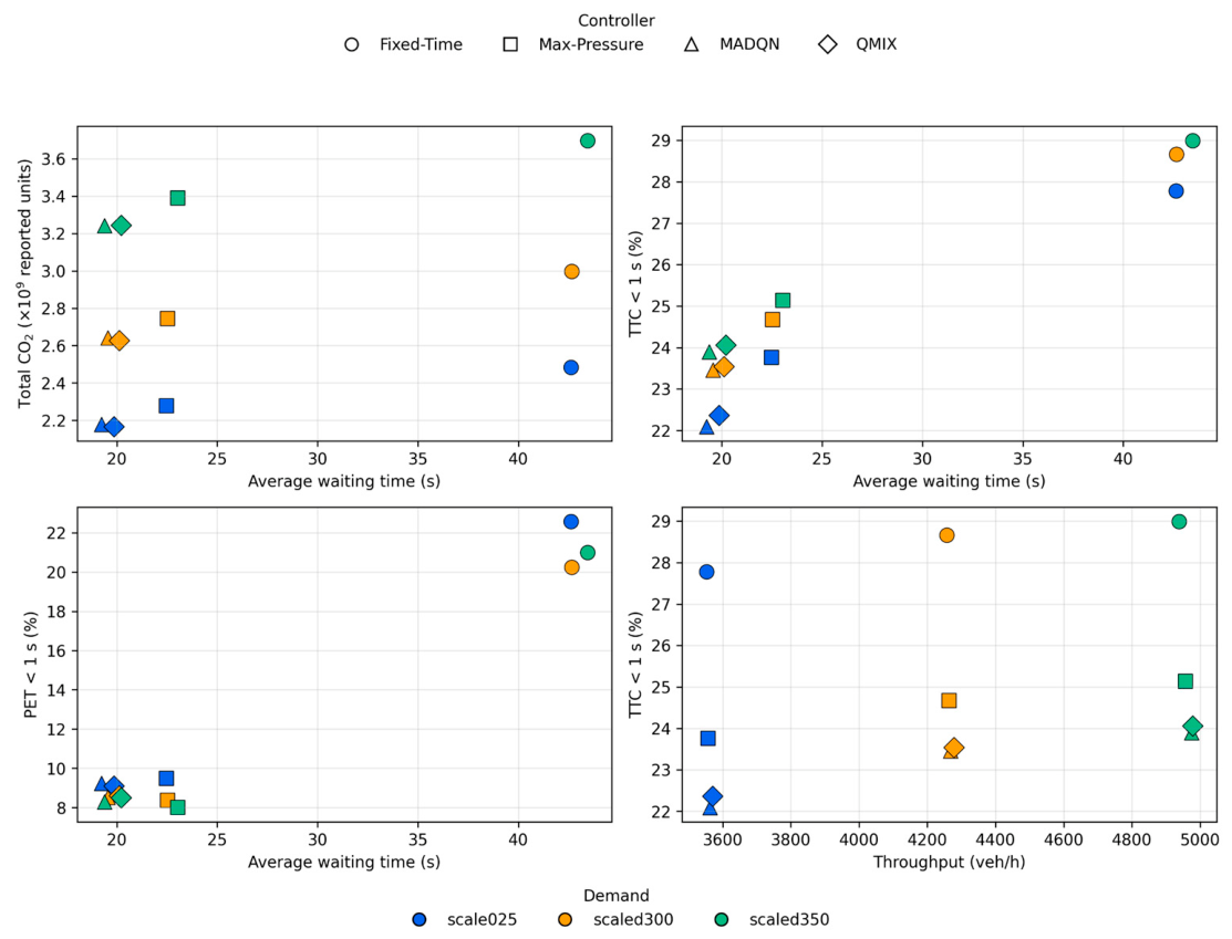
Stable gains across demand do not imply that any single controller is universally optimal when all criteria are considered jointly. Figure 10, therefore, interprets the results in a comparative multi-metric space rather than as a single-axis ranking. Under this reading, Fixed-Time offers no meaningful advantage: it is always worse, or near-worst, in waiting time, travel time, CO₂, TTC < 1 s, and PET < 1 s. Consequently, it is not on the practical decision frontier within the present mobility–environment–safety assessment.

Within the adaptive group, MADQN and QMIX form the main mobility–CO₂ emissions trade-off pair. In descriptive terms, MADQN generally achieved lower mean waiting time and lower TTC < 1 s ratios in the reported runs, making it attractive when delay minimization and severe TTC-based safety are prioritized in this testbed. QMIX, on the other hand, generally yielded higher throughput and often lower CO₂, particularly at low and medium demand, making it attractive when network discharge efficiency and environmental performance are emphasized. Neither RL controller strictly dominates the other in the current data, so the final preference depends on the weights assigned to delay minimization, throughput, and CO₂-related emissions.

Max-Pressure remains relevant as a trade-off baseline because safety is not one-dimensional. Although it is clearly weaker than the RL controllers in mobility and emissions, it yields the lowest PET < 1 s ratio at medium and high demand. From an applied perspective, this means that Max-Pressure remains attractive when interpretability, low online complexity, and a strong analytical control rule are valued over the additional training burden of RL. By contrast, MADQN may be preferred when a lower mean delay is prioritized in the present grid, whereas QMIX may be preferred when collective progression and descriptive-result stability are emphasized.

A limitation of these trade-off conclusions is that the RL controllers were not trained under identical reward and optimization setups, so their differences should not be interpreted as a pure causal effect of coordination alone. In addition, the evidence comes from a single synthetic 4 × 4 grid with a two-phase action space. These constraints narrow the scope of generalization and motivate broader topology, baseline, and reward-alignment studies in future work.

6. Conclusions

This manuscript examines the performance of the MADQN and QMIX multi-agent deep reinforcement learning algorithms on a 4 × 4 urban traffic network. The algorithms’ performance under varying traffic densities and density changes has been evaluated. The success of the algorithms has been assessed based on Fixed-Time control and Maximum-Pressure control. At the same time, results have been analyzed based on multi-objective criteria. Both reinforcement-learning controllers demonstrated a stable hierarchy, achieving positive results across combined mobility, emissions, and violence-based safety performance. In the reported experiments, this pattern was reflected by the fact that Fixed-Time produced the highest average waiting times across all three demand levels (42.62–43.45 s), whereas MADQN and QMIX reduced this range to about 19.24–20.21 s, while also keeping TTC < 1 s proportions below the Fixed-Time range of 27.78–29.00%.

The comparison between MADQN and QMIX showed that open coordination did not automatically and consistently yield better average mobility in the current test environment. While MADQN provided lower average waiting times and lower TTC-based severe interaction rates in the reported studies, QMIX offered higher efficiency, generally lower CO₂, and stronger descriptive cross-seed stability under heavier demand. However, the statistical superiority of MADQN over QMIX, or vice versa, has not been established. More specifically, after multiplicity correction, only the throughput difference at the low-demand level remained statistically significant, while the other MADQN–QMIX differences should be interpreted as directional comparative tendencies rather than broad superiority claims. However, the current study should be interpreted as a comparative evaluation of approaches under common working conditions and environments in the literature.

The comprehensive analysis also showed that the advantages of multi-agent reinforcement-learning control are not specific to a single operating point; they remained stable for both downward and upward demand shifts in the examined network. In a broader context, the study suggests that selecting controllers for urban traffic-signal control should be based not only on delay but also on clear operational priorities among mobility, environmental load, and surrogate safety.

Limitations and Future Work. The present findings should be interpreted within the scope of several study constraints. First, the experiments were conducted on a single synthetic 4 × 4 urban grid, so the reported controller hierarchy and trade-off patterns should not be assumed to transfer directly to arterial corridors, irregular urban layouts, or larger heterogeneous networks. Second, the control formulation used a simplified two-action phase space with common phase-validity constraints, which supported controlled comparison but did not represent the full diversity of signal-stage designs used in real deployments. Third, although MADQN and QMIX were evaluated under the same network, local observation basis, and decision interval, their implemented reward and optimization settings were not identical; therefore, the RL-versus-RL comparison should be interpreted as a comparison of implemented controllers rather than a pure isolation of coordination effects alone. Fourth, the demand model relied on fixed predefined routes and time-bounded flows rather than online rerouting or broader non-recurrent disturbances. Future work can extend the present study by incorporating reward-aligned reruns, evaluating additional topologies—such as arterial and mixed urban networks—developing richer phase and action formulations, introducing explicit incident- or accident-induced disturbance scenarios, and expanding baseline comparisons. Such extensions would help determine how stable the present MADQN–QMIX trade-offs remain under more diverse and realistic traffic-control settings.

References

1. Webster, F.V. Traffic Signal Settings; Road Research Technical Paper No. 39; Road Research Laboratory: London, UK, 1957. [Google Scholar]
2. Tang, D.; Duan, Y. Traffic signal control optimization based on neural network in the framework of model predictive control. Actuators 2024, 13, 251. [Google Scholar] [CrossRef]
3. Ouyang, C.; Zhan, Z.; Lv, F. A comparative study of traffic signal control based on reinforcement learning algorithms. World Electr. Veh. J. 2024, 15, 246. [Google Scholar] [CrossRef]
4. Rashid, T.; Samvelyan, M.; Schroeder de Witt, C.; Farquhar, G.; Foerster, J.; Whiteson, S. Monotonic value function factorisation for deep multi-agent reinforcement learning. J. Mach. Learn. Res. 2020, 21, 1–52. [Google Scholar]
5. Bouktif, S.; Cheniki, A.; Ouni, A.; El-Sayed, H. Deep reinforcement learning for traffic signal control with consistent state and reward design approach. Knowl.-Based Syst. 2023, 267, 110440. [Google Scholar] [CrossRef]
6. Tan, X.; Zhou, Y.; Jiao, X. Traffic signal control based on deep reinforcement learning using state fusion and trend reward. Eng. Appl. Artif. Intell. 2025, 159, 111701. [Google Scholar] [CrossRef]
7. Zhou, R.; Nousch, T.; Wei, L.; Wang, M. Constrained traffic signal control under competing public transport priority requests via safe reinforcement learning. Expert Syst. Appl. 2025, 284, 127676. [Google Scholar] [CrossRef]
8. Michailidis, P.; Michailidis, I.; Lazaridis, C.R.; Kosmatopoulos, E. Traffic Signal Control via Reinforcement Learning: A Review on Applications and Innovations. Infrastructures 2025, 10, 114. [Google Scholar] [CrossRef]
9. Graves, R.T.; Nelson, Z.E.; Chakraborty, S. A decentralized intersection management system through collaborative negotiation be-tween smart signals. J. Intell. Transp. Syst. 2023, 27, 272–294. [Google Scholar] [CrossRef]
10. Mushtaq, A.; Haq, I.U.; Sarwar, M.A.; Khan, A.; Khalil, W.; Mughal, M.A. Multi-Agent Reinforcement Learning for Traffic Flow Management of Autonomous Vehicles. Sensors 2023, 23, 2373. [Google Scholar] [CrossRef] [PubMed]
11. Fang, B.; Zheng, C.; Wang, H.; Yu, T. Two-Stream Fused Fuzzy Deep Neural Network for Multiagent Learning. IEEE Trans. Fuzzy Syst. 2023, 31, 511–520. [Google Scholar] [CrossRef]
12. Yang, X.; Yu, Y.; Feng, Y.; Ochieng, W.Y. Improving the Urban Transport System Resilience Through Adaptive Traffic Signal Control Enabled by Decentralised Multiagent Reinforcement Learning. J. Adv. Transp. 2024, 2024, 3035753. [Google Scholar] [CrossRef]
13. Han, G.; Liu, X.; Han, Y.; Peng, X.; Wang, H. CycLight: Learning traffic signal cooperation with a cycle-level strategy. Expert Syst. Appl. 2024, 255, 124543. [Google Scholar] [CrossRef]
14. Wei, H.; Chen, C.; Zheng, G.; Wu, K.; Gayah, V.; Xu, K.; Li, Z. PressLight: Learning max pressure control to coordinate traffic signals in arterial network. In Proceedings of the 25th ACM SIGKDD International Conference on Knowledge Discovery and Data Mining (KDD), Anchorage, AK, USA, 4–8 August 2019; pp. 1290–1298. [Google Scholar] [CrossRef]
15. Wei, H.; Xu, N.; Zhang, H.; Zheng, G.; Zang, X.; Chen, C.; Zhang, W.; Zhu, Y.; Xu, K.; Li, Z. CoLight: Learning network-level cooperation for traffic signal control. In Proceedings of the 28th ACM International Conference on Information and Knowledge Management (CIKM), Beijing, China, 3–7 November 2019; pp. 1913–1922. [Google Scholar] [CrossRef]
16. Ault, J.; Sharon, G. Reinforcement learning benchmarks for traffic signal control. In Proceedings of the 35th Conference on Neural Information Processing Systems (NeurIPS 2021) Datasets and Benchmarks Track, virtual, 6–14 December 2021; pp. 1–11. [Google Scholar]
17. Wei, H.; Zheng, G.; Gayah, V.; Li, Z. A survey on traffic signal control methods. arXiv 2019, arXiv:1904.08117. [Google Scholar]
18. Fan, L.; Yang, Y.; Ji, H.; Xiong, S. Research on cooperative control of traffic signals based on deep reinforcement learning. In Proceedings of the 2023 IEEE 12th Data Driven Control and Learning Systems Conference (DDCLS), Xiangtan, China, 12–14 May 2023; pp. 1608–1612. [Google Scholar] [CrossRef]
19. Rasheed, F.; Yau, K.-L.A.; Noor, R.M.; Chong, Y.-W. Deep reinforcement learning for addressing disruptions in traffic light control. Comput. Mater. Contin. 2022, 71, 2225–2247. [Google Scholar] [CrossRef]
20. Cao, K.; Yang, S.; Yang, C.; Yu, M.; Geng, J.; Jung, H. Research on intelligent traffic signal control based on multi-agent deep reinforcement learning. Mathematics 2026, 14, 149. [Google Scholar] [CrossRef]
21. Bokade, R.; Jin, X.; Amato, C. Multi-agent reinforcement learning based on representational communication for large-scale traffic signal control. IEEE Access 2023, 11, 47646–47658. [Google Scholar] [CrossRef]
22. Sattarzadeh, A.R.; Pathirana, P.N. Unification of probabilistic graph model and deep reinforcement learning (UPGMDRL) for multi-intersection traffic signal control. Knowl.-Based Syst. 2024, 305, 112663. [Google Scholar] [CrossRef]
23. Wang, L.; Zhang, W.; Yan, Z. Vehicle–infrastructure cooperation framework for vehicle navigation and traffic signal control using deep reinforcement learning. Transp. Res. Rec. 2026, 2680, 568–583. [Google Scholar] [CrossRef]
24. Zeynivand, A.; Javadpour, A.; Bolouki, S.; Sangaiah, A.K.; Ja’fari, F.; Pinto, P.; Zhang, W. Traffic flow control using multi-agent reinforcement learning. J. Netw. Comput. Appl. 2022, 207, 103497. [Google Scholar] [CrossRef]
25. Rasheed, F.; Yau, K.-L.A.; Low, Y.-C. Deep reinforcement learning for traffic signal control under disturbances: A case study on Sunway City, Malaysia. Future Gener. Comput. Syst. 2020, 109, 431–445. [Google Scholar] [CrossRef]
26. Kodama, N.; Harada, T.; Miyazaki, K. Traffic signal control system using deep reinforcement learning with emphasis on reinforcing successful experiences. IEEE Access 2022, 10, 128943–128950. [Google Scholar] [CrossRef]
27. Akbar, A.; Ullah, S.S.; Malik, A.; Qaisar, S.M. RT-FedFlow: An efficient framework for real-time traffic signal optimization using federated multi-agent reinforcement learning. Eng. Appl. Artif. Intell. 2025, 161, 112147. [Google Scholar] [CrossRef]
28. Hassan, M.A.; Elhadef, M.; Khan, M.U.G. Collaborative Traffic Signal Automation Using Deep Q-Learning. IEEE Access 2023, 11, 136016–136033. [Google Scholar] [CrossRef]
29. Guzmán, J.A.; Pizarro, G.; Núñez, F. A Reinforcement Learning-Based Distributed Control Scheme for Cooperative Intersection Traffic Control. IEEE Access 2023, 11, 57038–57046. [Google Scholar] [CrossRef]
30. An, Y.; Zhang, J. Traffic signal control method based on modified proximal policy optimization. In Proceedings of the 2022 10th International Conference on Traffic and Logistic Engineering (ICTLE), Macau, China, 12–14 August 2022. [Google Scholar] [CrossRef]
31. Meepokgit, T.; Wisayataksin, S. Traffic signal control with state-optimizing deep reinforcement learning and fuzzy logic. Appl. Sci. 2024, 14, 7908. [Google Scholar] [CrossRef]
32. Mei, X.; Fukushima, N.; Yang, B.; Wang, Z.; Takata, T.; Nagasawa, H.; Nakano, K. Reinforcement learning-based intelligent traffic signal control considering sensing information of railway. IEEE Sens. J. 2023, 23, 31125–31136. [Google Scholar] [CrossRef]
33. Bouktif, S.; Cheniki, A.; Ouni, A. Traffic signal control using hybrid action space deep reinforcement learning. Sensors 2021, 21, 2302. [Google Scholar] [CrossRef]
34. Xu, Y.; Wang, Y.; Liu, C. Training a reinforcement learning agent with AutoRL for traffic signal control. In Proceedings of the 2022 Euro-Asia Conference on Frontiers of Computer Science and Information Technology (FCSIT), Beijing, China, 16–18 December 2022. [Google Scholar] [CrossRef]
35. Wang, P.; Wu, X.; He, X. Vibration-Theoretic Approach to Vulnerability Analysis of Nonlinear Vehicle Platoons. IEEE Trans. Intell. Transp. Syst. 2023, 24, 11334–11344. [Google Scholar] [CrossRef]
36. Xu, D.; Liao, X.; Yu, Z.; Gu, T.; Guo, H. Robustness enhancement of deep reinforcement learning-based traffic signal control model via structure compression. Knowl.-Based Syst. 2025, 310, 113022. [Google Scholar] [CrossRef]
37. Jagdish, A.; Liu, T. Impact of reward function selection on DQN-based traffic signal control. In Proceedings of the 2024 IEEE International Conference on Green Energy and Smart Systems (GESS), Long Beach, CA, USA, 11–12 November 2024. [Google Scholar] [CrossRef]
Figure 1. Multi-Agent Deep Q-Netork (MADQN)-based signal control architecture.
Applsci 16 05008 g001
Figure 2. QMIX value-decomposition method (QMIX)-based signal control architecture.
Applsci 16 05008 g002
Figure 3. Experimental overview of the traffic-signal control study. Panel (a) shows the full 4 × 4 grid network comprising 16 signalized intersections. A representative central intersection is highlighted and enlarged in panel (b), which visualizes the local geometric layout and signalized approaches used by the controllers. Panel (c) shows the phase sequence used in each intersection.
Applsci 16 05008 g003
Figure 4. Training convergence for MADQN (left) and QMIX (right) over 400 episodes on the scaled300 demand scenario. Grey lines show per-episode mean travel time; colored lines show the 20-episode moving average. The green dashed line marks the best checkpoint selected for evaluation. Both controllers approach stable performance plateaus, suggesting that training had largely stabilized before evaluation.
Applsci 16 05008 g004
Figure 5. Baseline hierarchy across demand levels. The four panels compare Fixed-Time, Max-Pressure, MADQN, and QMIX under the three demand levels using average waiting time, average travel time, total CO2, and the proportion of very severe TTC events among logged TTC events (TTC < 1 s). Error bars indicate between-seed variability where available.
Applsci 16 05008 g005
Figure 9. Robustness across demand levels. The four panels report the percentage gain of each adaptive controller relative to the Fixed-Time baseline under the three demand scenarios for waiting time, travel time, total CO2, and TTC < 1 s.
Applsci 16 05008 g009
Figure 10. Multi-criteria trade-off structure across the four controllers. No controller is Pareto-optimal across all metric pairs: MADQN tends to yield lower mean waiting time, whereas QMIX tends to yield higher throughput and often lower CO2; Max-Pressure yields the lowest PET < 1 s ratios at medium and high demand despite its mobility deficit; and Fixed-Time is dominated in all panels.
Applsci 16 05008 g010