Satellite-Based Ground-Level NO₂ Estimation and Population Exposure Assessment Across the Marmara Region Using Tree-Based Machine Learning

Abstract

This study estimates daily nitrogen dioxide (NO₂) concentrations at ground level across the Marmara Region of Türkiye at 0.01° resolution. The framework integrates Sentinel-5P (S5P) TROPOspheric Monitoring Instrument (TROPOMI) and GEOS Composition Forecast (GEOS-CF) tropospheric NO₂ vertical column density (VCD) data with meteorological, topographic, land-use, socioeconomic, and temporal features through four tree-based ensemble algorithms trained on 74 ground station observations. Under a temporal split (2019–2022 training, 2023 validation, 2024 testing), S5P-Categorical Boosting (CatBoost) achieved the best performance (Pearson correlation coefficient (R) = 0.706, R² = 0.498, root mean square error (RMSE) = 14.31 µg/m³). Random splitting inflated R by +0.168 due to temporal autocorrelation, while leave-one-station-out and leave-one-province-out cross-validation reduced R to ~0.50 by removing spatial dependence, together revealing the combined effect of temporal and spatial autocorrelation. SHapley Additive exPlanations (SHAP) analysis identified TROPOMI NO₂ VCD, population density, road length, and nighttime light as dominant predictors; population density was the top predictor in the GEOS-CF model, followed by VCD. Concentration maps for 2024 showed that 95.9% of the region’s 26.74 million inhabitants were exposed above the WHO annual air quality guideline of 10 µg/m³, with a population-weighted mean of 21.08 µg/m³.

1. Introduction

Nitrogen dioxide (NO₂) is an atmospheric pollutant primarily emitted by fossil fuel combustion in the energy generation, industrial, on-road transportation, and international shipping sector [1]. Long-term NO₂ exposure has been linked to respiratory morbidity in adults, including asthma incidence [2] and chronic obstructive pulmonary disease hospital admissions [3]. Additionally, increased risks of all-cause, cardiovascular, and respiratory mortality have been observed [4,5]. These associations persist at concentrations well below major limit values, with no clear evidence for a concentration threshold [3,6,7]. These findings informed the 2021 World Health Organization (WHO) revision of the annual mean NO₂ air quality guideline (AQG) from 40 µg/m³ to 10 µg/m³ and the establishment of a 24 h AQG of 25 µg/m³ [8]. High-resolution ground-level NO₂ estimates are needed to quantify exposure, track progress toward these AQG levels, and guide air quality management.

Although ground-based monitoring stations have been widely used to obtain high-accuracy measurements of air quality at fixed sites [9,10], the high costs of establishing and operating these networks constrain their spatial coverage, resulting in sparse station distributions with limited population coverage that are disproportionately concentrated in urban areas [11,12,13]. Low-income countries remain underrepresented in monitoring networks [14], with only 5% of their populations residing within 5 km of a station compared to 60% in high-income countries [15]. These coverage gaps have prompted the adoption of spatially continuous data sources, particularly satellite remote sensing, to complement ground-based networks.

Satellite remote sensing offers a complementary means of monitoring atmospheric NO₂ with broad spatial coverage and regular temporal revisit cycles [16]. The TROPOspheric Monitoring Instrument (TROPOMI) aboard Sentinel-5P (S5P) provides the highest-resolution operational tropospheric NO₂ vertical column density (VCD) retrievals with near-daily global coverage at a spatial resolution sufficient to capture urban-scale variability [17,18]. Earlier processor versions exhibited substantial negative biases of up to −51% in the tropospheric column [19], which were partially addressed in subsequent updates that increased retrieved columns by 10–40% [20]. Data availability is limited primarily by cloud cover, whereas large winter solar zenith angles further reduce near-surface retrieval sensitivity [17,21]. TROPOMI VCDs nonetheless correlate increasingly with ground-level concentrations as the averaging period lengthens, from R ≈ 0.67–0.70 at daily to R ≈ 0.84 at annual scales, reaching 0.88 when excluding roadside stations [21,22]. TROPOMI measures column-integrated amounts rather than ground-level concentrations, so deriving ground-level estimates requires complementary data and modeling approaches.

Chemical transport models provide an additional source of spatially continuous NO₂ estimates. The GEOS Composition Forecast (GEOS-CF) system incorporates the GEOS-Chem chemistry module at 0.25° resolution to produce daily hindcasts and five-day forecasts, including both ground-level NO₂ fields and tropospheric NO₂ VCDs [23]. Unlike assimilative systems such as the Copernicus Atmosphere Monitoring Service [24], GEOS-CF operates without direct assimilation of tropospheric trace gas observations [25]; thus, its NO₂ VCD estimates are independent of satellite retrievals and suitable for use as a complementary predictor alongside TROPOMI data. However, the short photochemical lifetime of NO₂ generates steep concentration gradients near emission sources [26] that the 0.25° resolution of GEOS-CF may not fully resolve. Uncertainties in emission inventories and chemical mechanisms further limit model accuracy [23,27], motivating the integration of satellite observations with model and land-use data through data-driven approaches [18].

Conventional statistical methods, including multiple linear regression, land use regression, and geographically weighted regression, have been widely applied; however, their reliance on linear or locally linear specifications limits their capacity to represent the complex, nonlinear relationships underlying ground-level NO₂ variability [28]. Machine learning (ML) methods have generally demonstrated stronger predictive performance [29,30,31]; however, the margin of improvement narrows considerably under spatial and temporal evaluation strategies [11]. Ref. [31] found that the improvement of Random Forest (RF) and Support Vector Machine over a single-predictor linear model narrowed substantially when compared with a multiple linear regression using a largely overlapping predictor set, suggesting that a considerable portion of the improvement arose from additional predictors rather than nonlinear modeling capacity alone.

The predictive performance of ML-based models is also shaped by predictor composition. TROPOMI NO₂ VCD consistently emerges as the most influential predictor across different regions and methodologies [32,33,34]. It is typically complemented by population density (PD), land-use proxies, emission source indicators such as traffic volume and industrial point sources [35], nighttime light (NTL), the Normalized Difference Vegetation Index (NDVI) [36], and meteorological parameters [37]. In addition to predictor composition, the evaluation strategy itself influences reported performance: random train–test splitting is widely used in the air quality ML literature, inflating accuracy metrics because spatiotemporal autocorrelation introduces data leakage between training and test sets [29,38,39]. Replacing sample-based evaluation with random temporal splits or leave-one-year-out partitioning has been shown to reduce the coefficient of determination (R²) from 0.88 to 0.82 and 0.80, respectively, for satellite-based NO₂ [40]. Although these methodological refinements have improved the robustness of model evaluation, the geographical distribution of satellite-based ground-level NO₂ studies remains highly imbalanced, with the majority originating from China, Europe, and the US; regions with limited monitoring infrastructure are significantly underrepresented [41].

Türkiye is underrepresented in this literature despite ranking among the 20 most populous countries and recording increased annual NO₂ concentrations from 2013 to 2023 [42]. Having undergone rapid urbanization over recent decades, with approximately 90% of its population now residing in urban areas [43], Türkiye faces elevated and spatially heterogeneous NO₂ exposure that necessitates high-resolution monitoring. Existing air quality research relevant to NO₂ in Türkiye has focused on lockdown impact evaluation [44], deep learning-based station-level forecasting [45], and spatiotemporal characterization [46]. Importantly, none of these studies employed satellite-derived NO₂ VCDs within an ML-based ground-level estimation framework or generated gridded ground-level NO₂ fields. Recently, the first such approach, to our knowledge, was provided for Istanbul [47], employing three tree-based algorithms (RF, Extreme Gradient Boosting (XGBoost) and Categorical Boosting (CatBoost)) with S5P TROPOMI and GEOS-CF inputs. The best-performing model (CatBoost) achieved a Pearson correlation coefficient (R) of 0.686 and a root mean square error (RMSE) of 16.23 µg/m³; however, this study was limited to a single metropolitan area.

The present study extends [47] both geographically and methodologically to all 11 provinces of the Marmara Region, estimating ground-level NO₂ at a 0.01° (~1 km) resolution. Models are trained using ground-based observations from 2019 to 2022, validated on data from 2023, and applied to generate region-wide seasonal and annual concentration maps for 2024. The study area encompasses dense urban centers (Istanbul, Bursa), heavy-industry corridors (Kocaeli petrochemicals, Bursa automotive), agricultural areas (Edirne, Balikesir, Canakkale), and rural zones, enabling performance assessment across a considerably wider range of land-use and emission regimes than permitted by a single-city setting. This study makes four principal contributions: (i) S5P TROPOMI and GEOS-CF NO₂ VCDs are integrated with meteorological, topographic, land-use, environmental, socioeconomic, and temporal predictors (selected through a multicollinearity diagnostic procedure), enabling the relative utility of two column sources with disparate spatial resolutions to be quantified; (ii) four tree-based ensemble algorithms (RF, XGBoost, CatBoost, Light Gradient Boosting Machine (LightGBM)) are benchmarked under hyperparameter optimization, with model behavior interpreted using SHapley Additive exPlanations (SHAP) analysis; (iii) both temporal and random splitting strategies are applied to explicitly quantify data leakage effects; and (iv) high-resolution (~1 km) seasonal NO₂ maps across the region are evaluated against the WHO revised AQG levels [8] to assess the spatial and seasonal distribution of population exposure.

2. Materials and Methods

2.1. Study Area

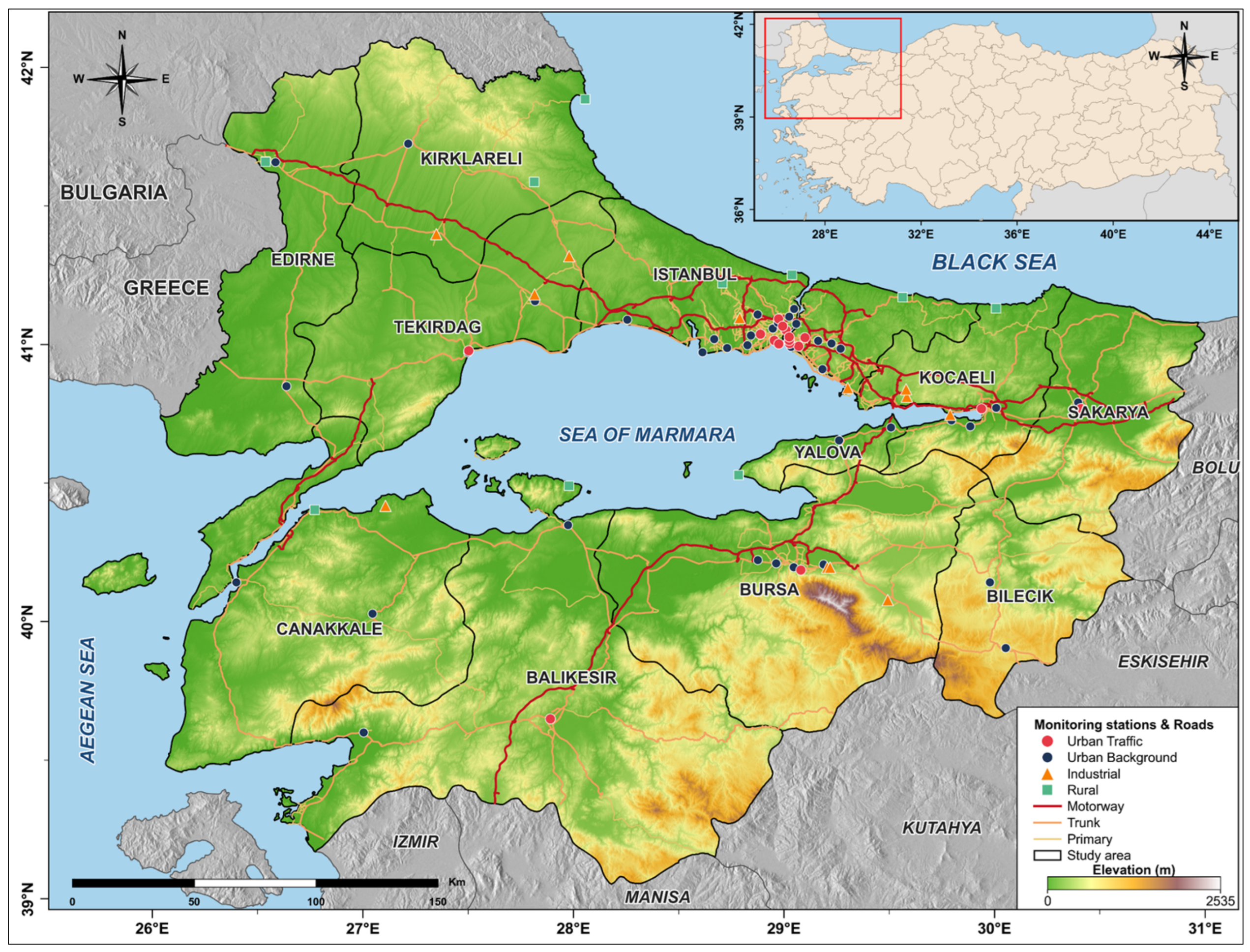
The Marmara Region is situated in northwestern Türkiye, between approximately 39°04′ N–42°06′ N and 25°40′ E–31°01′ E, and encompasses 11 provinces: Istanbul, Bursa, Kocaeli, Tekirdag, Balikesir, Sakarya, Yalova, Bilecik, Canakkale, Edirne, and Kirklareli. It covers an area of approximately 72,000 km², i.e., 9.2% of Türkiye’s total land area, and is bordered by the Black Sea to the north and the Aegean Sea to the west; the Sea of Marmara is at its center (Figure 1). Although it has the lowest average elevation among Türkiye’s geographical regions, the terrain exhibits considerable heterogeneity, ranging from coastal lowlands to mountain peaks exceeding 2500 m. These topographic contrasts, coupled with the moderating influence of the surrounding seas, produce a transitional climate with Mediterranean and Black Sea influences [48,49].

With a population of approximately 26.74 million, 31% of Türkiye’s total population [50], Marmara is the country’s most densely populated and economically dominant region, accounting for 48% of the national industrial share [51]. Manufacturing activities in the automotive, textile, cement, food processing, and petrochemical sectors are concentrated along two main corridors: one running from Istanbul, the economic core of the region, through Kocaeli to Bursa, and another linking Tekirdag with Kirklareli [46]. Further east, the Izmit Bay area in Kocaeli is one of the most intensively industrialized provinces in the country, hosting 14 organized industrial zones [52] and accumulating a high density of industrial establishments, including major enterprises and smaller production plants [53]. Bursa, the second most populous province, hosts a diverse industrial base whose emissions have been identified as the leading contributor to its air pollution problem [54]. This concentration of industrial activity, coupled with rapid urbanization and growing transport demand, has led to substantial nitrogen oxides (NO_x) emissions from both land-based and maritime sources. The study area hosts approximately 10.7 million registered motor vehicles [50]; combined with its physical and climatic diversity, these emissions are expected to produce considerable spatial and temporal variability in ground-level NO₂ concentrations, making the region well suited for evaluating satellite-based NO₂ estimation approaches.

2.2. Datasets

The datasets used herein originate from satellite remote sensing and atmospheric reanalysis products accessed through Google Earth Engine (GEE), ground-based air quality measurements from the Turkish Ministry of Environment, Urbanization and Climate Change (MoEUCC) [55], and other publicly available ancillary sources, covering the period January 2019 to December 2024. Input and output variables are summarized in

Table 1. Summary of input and output variables used for ground-level NO₂ estimation.

Category	Name	Variable	Spatial Resolution	Temporal Resolution	Source	Role
Satellite and Reanalysis	S5P TROPOMI	Tropospheric NO2 VCD	~1 km	Daily	GEE	Input
	GEOS-CF	Tropospheric NO2 VCD	~0.25°	Hourly	GEE	Input
		Dust optical depth at 550 nm (AOD550_DUST)
		Surface geopotential height (PHIS)
		Surface pressure (PS)
		Specific humidity (Q)
		Relative humidity (RH)
		Sea level pressure (SLP)
		2 m Air temperature (T2M)
		Total precipitation (TPREC)
		Surface skin temperature (TS)
		10 m Eastward wind (U10M)
		10 m Northward wind (V10M)
		Mid-layer heights (ZL)
		Planetary boundary layer height (ZPBL)
	MODIS MCD43A4	NDVI	500 m	Daily	GEE	Input
	VIIRS VNP46A2	NTL	500 m	Daily	GEE	Input
	SRTM	Digital elevation model (DEM)	30 m	Static	GEE	Input
Ground-Based and Ancillary	Air Quality Stations	NO2 concentration (µg/m3)	Point	Hourly	MoEUCC	Output
	OpenStreetMap	RL	Vector	Static	Geofabrik	Input
	TÜİK	PD	District	Annual	TÜİK	Input
	Derived	DOY_sin, DOY_cos	-	Daily	Calculated	Input
		wind_speed			Derived from GEOS-CF

, and preprocessing steps are detailed in Section 3.

2.2.1. Satellite and Reanalysis Data

Five datasets accessed through GEE were used as the main set of input variables for estimating ground-level NO₂ concentrations across Marmara. The primary satellite NO₂ input was obtained from the S5P TROPOMI Level-3 offline tropospheric NO₂ VCD product, available at a nadir footprint of 3.5 × 5.5 km² since 6 August 2019 with one daytime overpass per day at ~13:30 local time [17] and stored at a spatial sampling of approximately 1 km in GEE. As an alternative column source, the GEOS-CF hindcast product (~0.25°) provided a second, independent tropospheric NO₂ VCD. The same product also supplied 13 atmospheric variables (AOD550_DUST, PHIS, PS, Q, RH, SLP, T2M, TPREC, TS, U10M, V10M, ZL, and ZPBL). In addition to the column and meteorological inputs, three further variables derived from GEE datasets were included to capture spatial and environmental heterogeneity: NDVI derived from the Moderate Resolution Imaging Spectroradiometer (MODIS) nadir-corrected reflectance product [56] as a vegetation cover indicator, NTL from the Visible Infrared Imaging Radiometer Suite (VIIRS) gap-filled product [57] as a proxy for the intensity of anthropogenic activity, and terrain elevation from the Shuttle Radar Topography Mission (SRTM) DEM [58].

2.2.2. Ground-Based and Ancillary Data

MoEUCC operates 92 ground-based air quality monitoring stations across the study area, of which 77 provided NO₂ measurements. After excluding three stations lacking sufficient data across all training, validation, and test periods, we retained 74 stations for model development: Istanbul (33), Kocaeli (8), Bursa (7), Tekirdag (4), Canakkale (4), Kirklareli (4), Sakarya (3), Edirne (3), Yalova (3), Balikesir (3), and Bilecik (2). This network of stations covers areas ranging from dense urban corridors to semi-rural inland districts. To complement these point-based observations with spatially explicit ancillary information, road length (RL) was derived from OpenStreetMap data [59] as a proxy for traffic-related emission density, and PD was calculated using annual district-level population figures [50]. The day of year (DOY) was additionally included as a temporal variable. For spatial prediction, a 0.01° × 0.01° (~1 km) regular grid was generated over the study area; the grid construction procedure and variable assignment strategy are described in Section 3.

3. Methodology

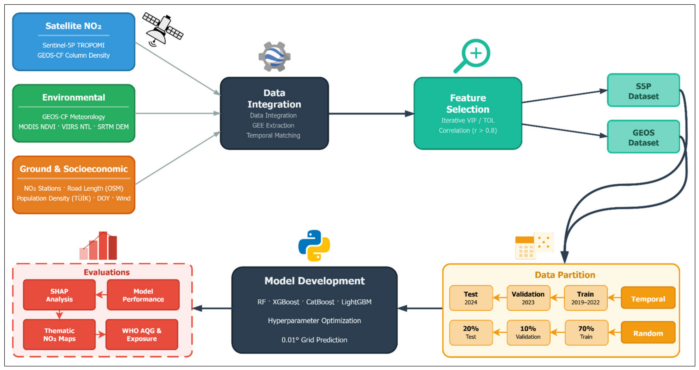
This study was conducted in three parts: data preprocessing and feature extraction, model development using ML algorithms, and model evaluation. The complete workflow, including temporal filtering and quality masking through hyperparameter optimization and SHAP analysis, is summarized in Figure 2 and detailed in the following subsections.

3.1. Data Preprocessing and Feature Extraction

Due to the different acquisition schedules and spatial resolutions of the datasets used, a temporal and spatial harmonization procedure was applied. Each source was converted to daily resolution for the 2019–2024 period: S5P observations were averaged over the 10:00–13:00 UTC window using pixels with cloud fraction below 0.3 and GEOS-CF variables were filtered to 11:00–12:00 UTC and averaged per day. Ground-level NO₂ records were averaged to one value per station per day within the 14:00–15:00 local time window. These time windows were selected to approximate the S5P local overpass time (~13:30 local time, ~10:30 UTC). MODIS NDVI and VIIRS NTL images were used at daily resolution, and a long-term mean was computed for the grid. All variables were spatially matched to station locations using GEE at a scale of 1000 m. Records with ground-level NO₂ outside 1–300 µg/m³ or with missing values were excluded, following [34]. This removed 2.50% of the 289,929 hourly observations within the 14:00–15:00 local time window (2.499% below 1 µg/m³, 0.002% above 300 µg/m³), retaining 282,679 records. The retained pooled distribution had a median of 16.35 µg/m³ (P25 = 7.31, P75 = 32.11, P95 = 67.60 µg/m³). The formulations of the features derived from the remaining data after quality control are shown in

Table 2. Derived features and their formulations.

Feature	Formula	Definition
NDVI	${\displaystyle \frac{\mathrm{Band} 2-\mathrm{Band} 1}{\mathrm{Band} 2+\mathrm{Band} 1}}$	Band 2 (Near-Infrared) and Band 1 (Red) from MODIS
wind_speed	$\sqrt{U_{10M}^2+V_{10M}^2}$	$U_{10M}$, $V_{10M}$: GEOS-CF 10 m wind components
DOY_sin DOY_cos	$\sin \left({\displaystyle \frac{2\pi \mathrm{DOY}}{365}}\right)$ $\cos \left({\displaystyle \frac{2\pi \mathrm{DOY}}{365}}\right)$	DOY: day of year

. Among these, RL was obtained by computing the total length (km) of road segments within each 0.01° cell. PD was assigned to stations via point-in-polygon matching at the district level. At grid level, area-weighted averaging was used where cells overlap multiple districts.

3.2. Feature Selection

Satellite and reanalysis features were derived from sensors and models operating at comparable spatial resolutions, and intercorrelation among input features was expected due to physical coupling between the underlying atmospheric and meteorological quantities. To address this multicollinearity before model training, we implemented a two-stage feature selection procedure. In the first stage, we performed an iterative elimination based on Variance Inflation Factor (VIF) and Tolerance (TOL). A VIF above 10 or TOL below 0.1 is generally regarded as indicative of multicollinearity [60,61], a threshold also widely adopted in satellite-based NO₂ estimation studies [62,63]. Based on these thresholds, the feature with the highest VIF was removed and the VIF values were recalculated; this process continued until all remaining features satisfied both criteria. In the second stage, pairwise Pearson correlation coefficients were calculated among the features that passed the first stage. For any pair with an absolute correlation exceeding 0.8 [64], the feature with the higher VIF, recalculated at each iteration, was removed. After each removal, the correlation matrix was recomputed, and this process was repeated until no pairwise correlations exceeded the threshold. The features retained after both stages constituted the final feature sets used for model training.

3.3. Data Splitting and Validation Strategies

Two data-splitting strategies were used to evaluate the performance of four algorithms (RF, XGBoost, CatBoost, and LightGBM). In temporal splitting, we used the period 2019–2022 for training, 2023 for validation, and 2024 for testing, ensuring that predictions relied solely on past observations. In random splitting, we partitioned the entire dataset into training, validation, and test subsets in a 70/10/20% ratio without preserving temporal order, allowing us to quantify the artificial performance inflation caused by spatiotemporal autocorrelation between the training and test samples. For both strategies, we applied each algorithm to the S5P- and GEOS-CF-based feature sets, yielding a total of 16 model configurations. To complement these temporal evaluation strategies, two spatial cross-validation procedures were applied: leave-one-station-out (LOSO, 74 folds) and leave-one-province-out (LOPO, 11 folds). LOSO holds out a single station at a time and trains on the remaining 73 stations, evaluating prediction accuracy at the held-out site. LOPO holds out all stations within a single province and trains on the remaining 10 provinces, providing a stricter test of transfer to entirely unseen regional contexts. In both procedures, the optimal hyperparameters identified under the temporal split were used, with the number of iterations held fixed. Spatial cross-validation was applied to the best-performing model configuration of each feature set.

3.4. Machine Learning Algorithms

We selected four tree-based ensemble algorithms that have been widely applied in satellite-based air quality estimation [29,30,31]. Deep learning alternatives were not considered, as: (i) tree-based models consistently outperform deep learning methods in tabular prediction tasks while requiring significantly less computation and hyperparameter tuning [65,66], a pattern also observed in air quality prediction applications [67]; (ii) the spatially distributed nature of our data (74 stations) makes the problem more akin to spatial generalization than long-term sequential forecasting, which is the primary advantage of recurrent architectures; and (iii) tree-based models handle heterogeneous predictors (continuous, cyclical, categorical) without the preprocessing pipelines required by neural networks.

RF constructs an ensemble of decision trees, each of which is trained on a bootstrap sample with a random feature subset at each split [68]. Unlike RF, XGBoost builds trees sequentially in an additive manner, with each new tree fitted under a regularized objective function [69]. LightGBM follows the same sequential boosting framework, but introduces sampling and feature bundling techniques to reduce training costs when applied to high-dimensional data [70]. CatBoost addresses biased gradient estimates through permutation-based training and employs oblivious decision trees, where a single splitting criterion is applied across an entire level, as base learners [71].

3.5. Hyperparameter Optimization

The hyperparameters of each algorithm were tuned using the Optuna framework [72], which employs a Tree-structured Parzen Estimator sampler to guide the search toward promising regions of parameter space. This sampling strategy has advantages over grid or random search, since Bayesian optimization methods typically achieve higher sampling efficiency [73,74]. For each algorithm-feature set combination, Optuna executed 200 trials aiming to minimize the validation RMSE. The search space covered tree structure parameters such as maximum depth and number of estimators, regularization terms, learning rate, and subsampling ratios, with the specific set varying by algorithm. To prevent unnecessary iterations during the boosting process, an early stopping criterion of 50 rounds was applied to XGBoost, CatBoost, and LightGBM. The optimal configuration identified for each combination was then used to train the final models.

3.6. Model Evaluation and Accuracy Assessment

To evaluate the predictive performance of the developed models, the agreement between modeled and measured NO₂ concentrations was assessed using four statistical metrics: R, R², RMSE, and mean absolute error (MAE) (Equations (1)–(4)). Although R shows no consistent relationship with prediction accuracy and has been criticized as a standalone evaluation metric [75], it remains widely reported alongside error metrics in the satellite-based NO₂ literature [30,76,77]. RMSE and MAE were included to provide the error characterization that R lacks. The statistical metrics were computed as follows:

$$\mathrm{R}={\displaystyle \frac{{\sum }_{\mathrm{i}=1}^{\mathrm{n}}\left({\mathrm{x}}_{\mathrm{i}}-{\mathrm{x}}_{\mathrm{m}}\right)\left({\widehat{\mathrm{x}}}_{\mathrm{i}}-{\widehat{\mathrm{x}}}_{\mathrm{m}}\right)}{\sqrt{{\sum }_{\mathrm{i}=1}^{\mathrm{n}}{\left({\mathrm{x}}_{\mathrm{i}}-{\mathrm{x}}_{\mathrm{m}}\right)}^2{\sum }_{\mathrm{i}=1}^{\mathrm{n}}{\left({\widehat{\mathrm{x}}}_{\mathrm{i}}-{\widehat{\mathrm{x}}}_{\mathrm{m}}\right)}^2}}}$$

(1)

$${\mathrm{R}}^2=1-{\displaystyle \frac{{\sum }_{i=1}^n{\left(x_i-{\widehat{x}}_i\right)}^2}{{\sum }_{i=1}^n{\left(x_i-x_m\right)}^2}}$$

(2)

$$\mathrm{R}\mathrm{M}\mathrm{S}\mathrm{E}=\sqrt{{\displaystyle \frac{{\sum }_{i=1}^n{\left(x_i-{\widehat{x}}_i\right)}^2}{n}}}$$

(3)

$$\mathrm{M}\mathrm{A}\mathrm{E}={\displaystyle \frac{{\sum }_{i=1}^n\left|x_i-{\widehat{x}}_i\right|}{n}}$$

(4)

where $x_i$ and ${\widehat{x}}_i$ denote the observed and predicted concentrations, $x_m$ and ${\widehat{x}}_m$ denote the means of the respective observed and predicted series, and $n$ denotes the number of samples. We computed all four metrics on the training, validation, and test sets for each of the 16 configurations. Among these, we selected the best-performing configuration based on the lowest validation RMSE under the temporal split.

3.7. SHapley Additive exPlanations

ML models, including tree-based ensembles, operate as black-box systems whose internal decision mechanisms are not directly interpretable [78]. SHAP was used to quantify individual feature attributions; the physical plausibility of the resulting attribution patterns was assessed by comparing them with known atmospheric and emission processes. SHAP is grounded in the Shapley value concept from cooperative game theory, where each input feature is treated as a player and the model prediction as the outcome attributed. SHAP computes the marginal contribution of each feature across all possible feature subsets and averages these contributions to obtain a single attribution value per feature. Shapley values are the only additive feature attribution method satisfying local accuracy, missingness, and consistency simultaneously [79]. Exact computation requires all possible feature subsets to be evaluated; thus, the TreeExplainer algorithm, which exploits the internal structure of tree-based models to achieve polynomial-time computation in place of the exponential cost of exact evaluation, was employed instead [80]. SHAP analysis was applied to the model that achieved the highest predictive accuracy according to the evaluation metrics defined in Section 3.6. In addition to overall feature rankings, yearly rankings were computed to evaluate temporal stability, with agreement between years quantified using the Spearman rank correlation coefficient (ρ).

4. Results

4.1. Multicollinearity

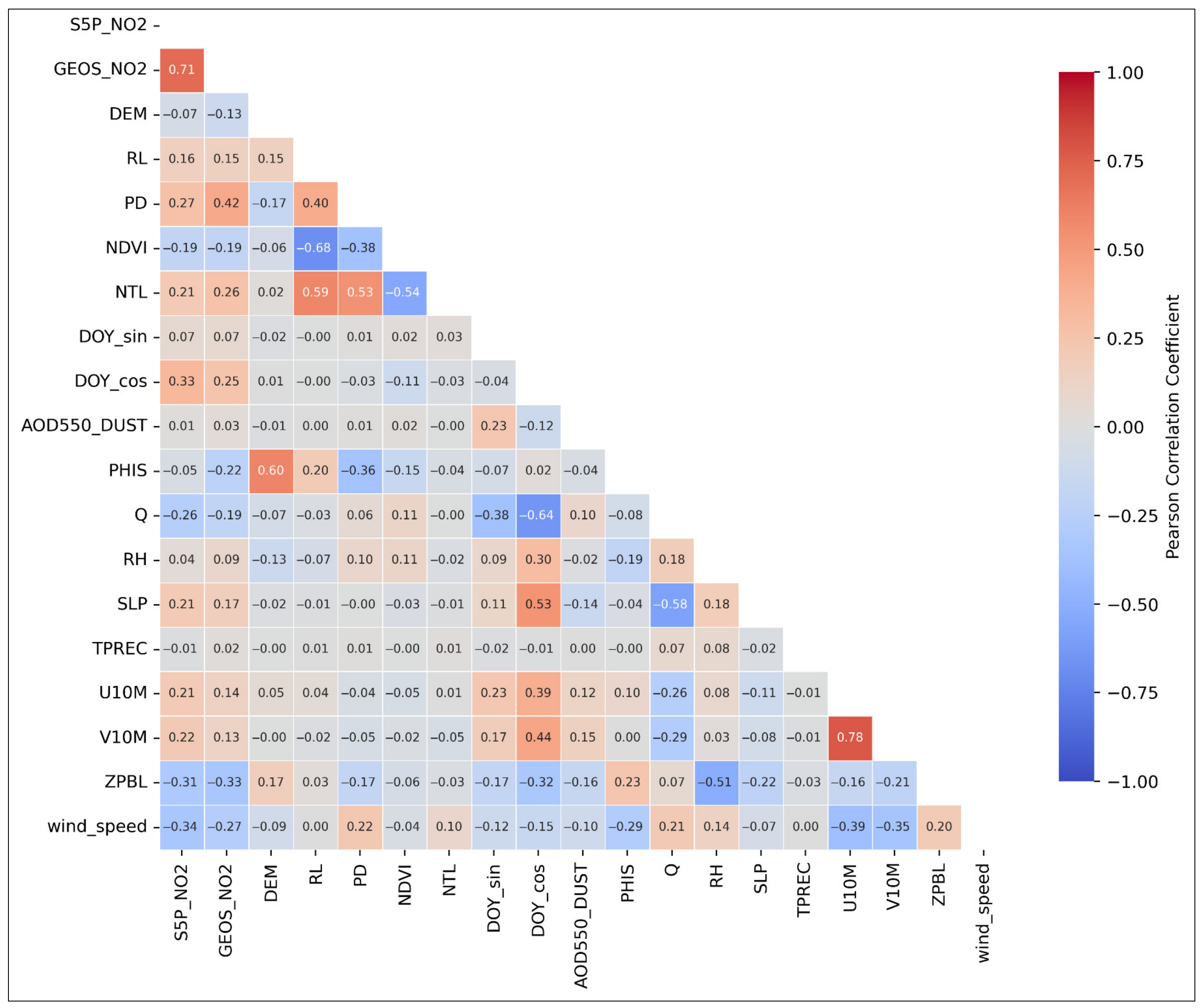
We applied the two-stage elimination procedure described in Section 3.2 to the initial set of 23 features. During the first stage, VIF and TOL values were calculated and the feature with the highest VIF exceeding predefined thresholds (VIF > 10, TOL < 0.1) was removed at each step, after which all values were recalculated. This process eliminated four GEOS-CF-derived meteorological features: ZL (VIF = 278.02), T2M (VIF = 53.43), PS (VIF = 21.00), and TS (VIF = 11.40). The particularly high VIF of ZL reflects its strong collinearity with elevation-related variables, whereas T2M and TS were redundant with each other, both capturing surface temperature. The VIF values of the 19 retained features ranged from 1.01 to 5.82, all within the predefined thresholds. We then examined their pairwise Pearson correlation coefficients, the highest of which was 0.779, below the 0.8 threshold. The procedure thus retained 19 of the initial 23 features, with a maximum VIF of 5.82 corresponding to DOY_cos. The final feature set incorporates column density, meteorological, environmental, topographic, socioeconomic, and temporal domains, as outlined in Table 1, and the correlation matrix of the final feature set is shown in Figure 3.

4.2. Model Training and Performance Evaluation

Under the random split, all models achieved high test accuracy, with R values ranging from 0.827 (GEOS-CF CatBoost) to 0.869 (S5P XGBoost) and RMSE ranging from 10.75 to 12.23 µg/m³ (

Table 3. Model performance under the random split (RMSE and MAE values are in µg/m³).

Feature Set	Model	Train				Validation				Test
		R	R2	RMSE	MAE	R	R2	RMSE	MAE	R	R2	RMSE	MAE
S5P	RF	0.949	0.901	7.249	4.462	0.833	0.694	12.106	7.240	0.841	0.706	11.771	7.328
	XGBoost	0.981	0.962	4.465	2.938	0.865	0.749	10.979	6.595	0.869	0.755	10.751	6.701
	CatBoost	0.919	0.845	8.804	5.923	0.841	0.707	11.885	7.406	0.844	0.712	11.675	7.543
	LightGBM	0.963	0.927	6.113	4.320	0.864	0.747	11.002	6.756	0.869	0.755	10.750	6.786
GEOS-CF	RF	0.958	0.919	6.706	4.190	0.830	0.689	12.217	7.426	0.836	0.698	11.949	7.511
	XGBoost	0.985	0.970	4.049	2.553	0.861	0.742	11.124	6.758	0.863	0.744	10.999	6.853
	CatBoost	0.903	0.815	9.652	6.457	0.830	0.689	12.264	7.770	0.827	0.685	12.230	7.935
	LightGBM	0.960	0.921	6.364	4.356	0.861	0.741	11.138	6.854	0.862	0.743	11.011	6.937

). S5P-based models outperformed their GEOS-CF counterparts across all four algorithms. Differences among algorithms were more pronounced than under the temporal split, with XGBoost and LightGBM achieving the lowest RMSE values in both feature sets.

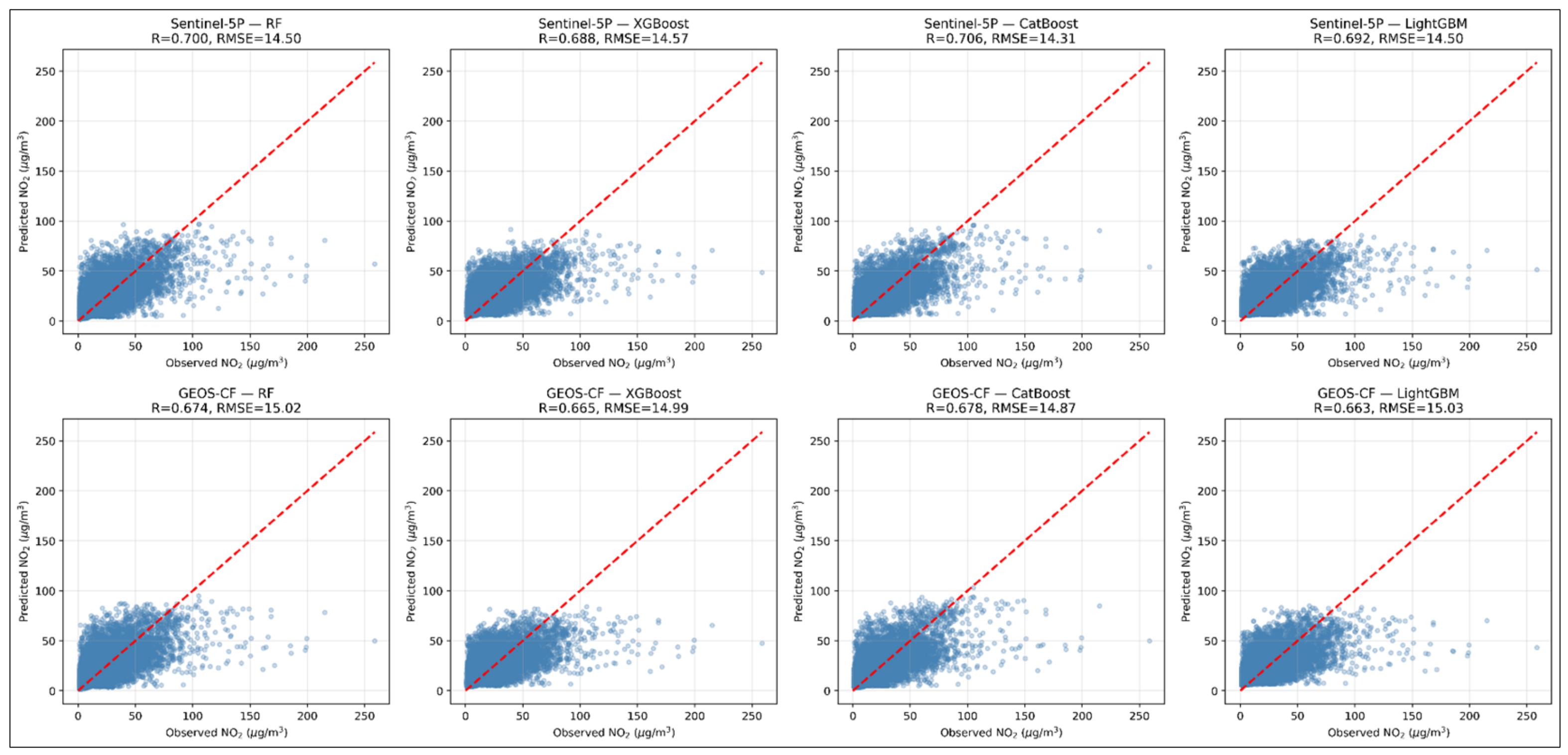
The temporal split (2019–2022 for training, 2023 for validation, and 2024 for testing) revealed a substantial drop in model performance (

Table 4. Model performance under the temporal split (RMSE and MAE values are in µg/m³).

Feature Set	Model	Train				Validation				Test
		R	R2	RMSE	MAE	R	R2	RMSE	MAE	R	R2	RMSE	MAE
S5P	RF	0.883	0.780	11.000	7.035	0.741	0.549	13.828	9.475	0.700	0.491	14.503	9.460
	XGBoost	0.947	0.896	8.793	5.782	0.741	0.549	13.664	9.335	0.688	0.473	14.567	9.616
	CatBoost	0.853	0.728	12.335	8.214	0.752	0.566	13.510	9.445	0.706	0.498	14.313	9.508
	LightGBM	0.890	0.792	11.128	7.430	0.737	0.543	13.744	9.433	0.692	0.478	14.501	9.486
GEOS-CF	RF	0.898	0.806	10.372	6.457	0.722	0.522	14.134	9.545	0.674	0.454	15.016	9.783
	XGBoost	0.914	0.835	10.157	6.422	0.721	0.520	13.998	9.384	0.665	0.442	14.988	9.756
	CatBoost	0.848	0.718	12.385	8.152	0.732	0.536	13.870	9.519	0.678	0.460	14.874	9.737
	LightGBM	0.886	0.785	11.370	7.574	0.717	0.514	14.120	9.644	0.663	0.439	15.033	9.899

). Test R values for the S5P feature set fell to 0.688–0.706 while RMSE rose to 14.31–14.57 µg/m³. GEOS-CF models followed the same trend, with test R values of 0.663–0.678 and RMSE values of 14.87–15.03 µg/m³. The average R inflation between the two splits was +0.168 and the average RMSE reduction was 3.33 µg/m³. The inflation was largest for XGBoost and LightGBM in both feature sets (ΔR = +0.181/+0.177 for S5P, +0.198/+0.199 for GEOS-CF). All subsequent analyses are therefore based on the temporal split.

The temporal split results revealed relatively small differences among the four algorithms within each feature set. For the S5P models, the test RMSE spanned only 0.25 µg/m³ between the best (CatBoost, 14.31) and worst (XGBoost, 14.57) performers, and test R values varied by just 0.018. GEOS-CF models exhibited even more limited spread, with test RMSE confined to a 0.16 µg/m³ range and near-identical R values around 0.67. All 16 configurations produced RMSE values below the standard deviation of the corresponding target set (training: 22.68, validation: 20.13, testing: 20.01 µg/m³). Based on the lowest validation RMSE, S5P-based CatBoost was identified as the best-performing configuration (test R = 0.706, R² = 0.498, RMSE = 14.31 µg/m³, MAE = 9.51 µg/m³). Scatter plots of predicted versus observed NO₂ concentrations for all temporal test configurations are shown in Figure 4. Across all model configurations, the majority of predictions clustered within the 0–50 µg/m³ range. Models tended to overestimate at observed concentrations below approximately 25 µg/m³ and progressively underestimate at higher concentrations, irrespective of algorithm or feature set.

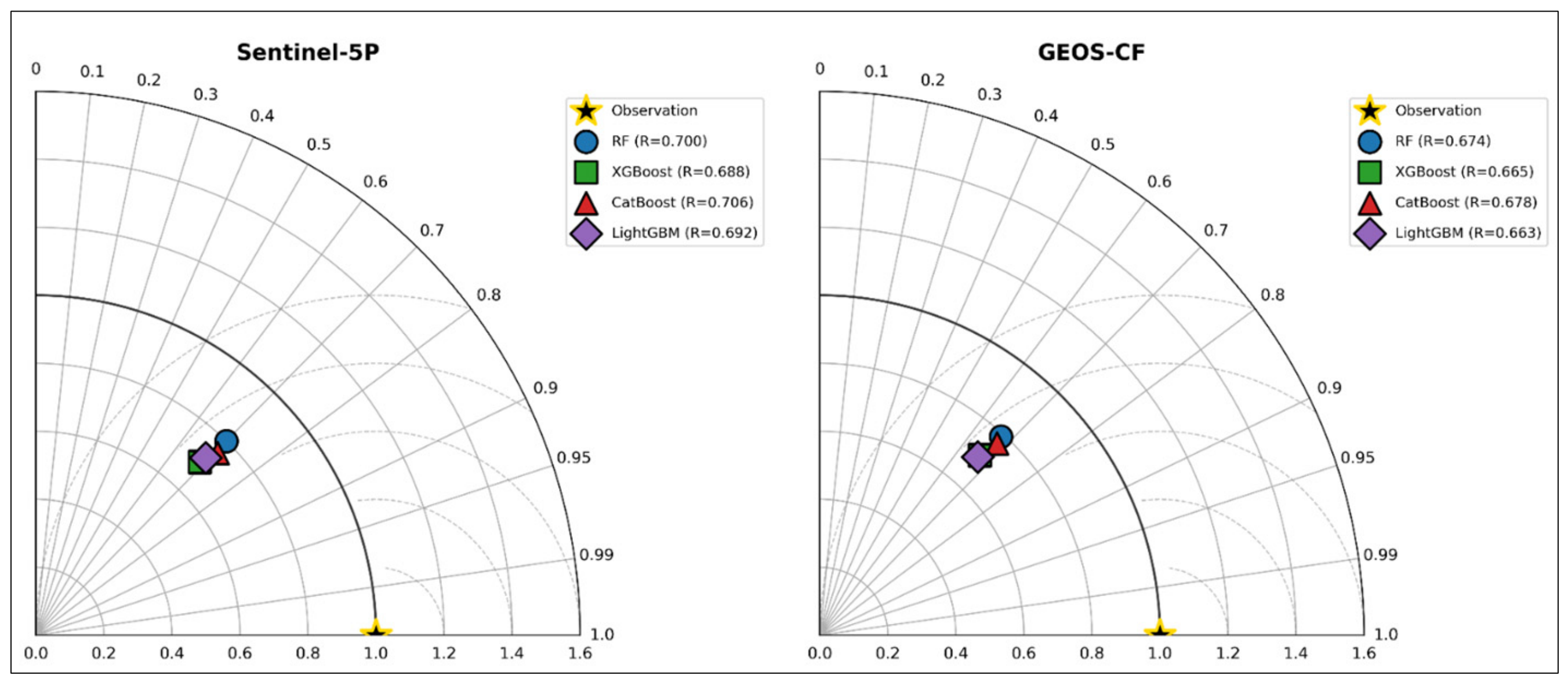
Taylor diagrams were used to further examine model behavior under the temporal split (Figure 5). All eight configurations underestimated the observed variability, with standard deviation ratios between 0.700 (GEOS-CF LightGBM) and 0.800 (S5P RF). S5P-based models showed marginally higher correlations than GEOS-CF.

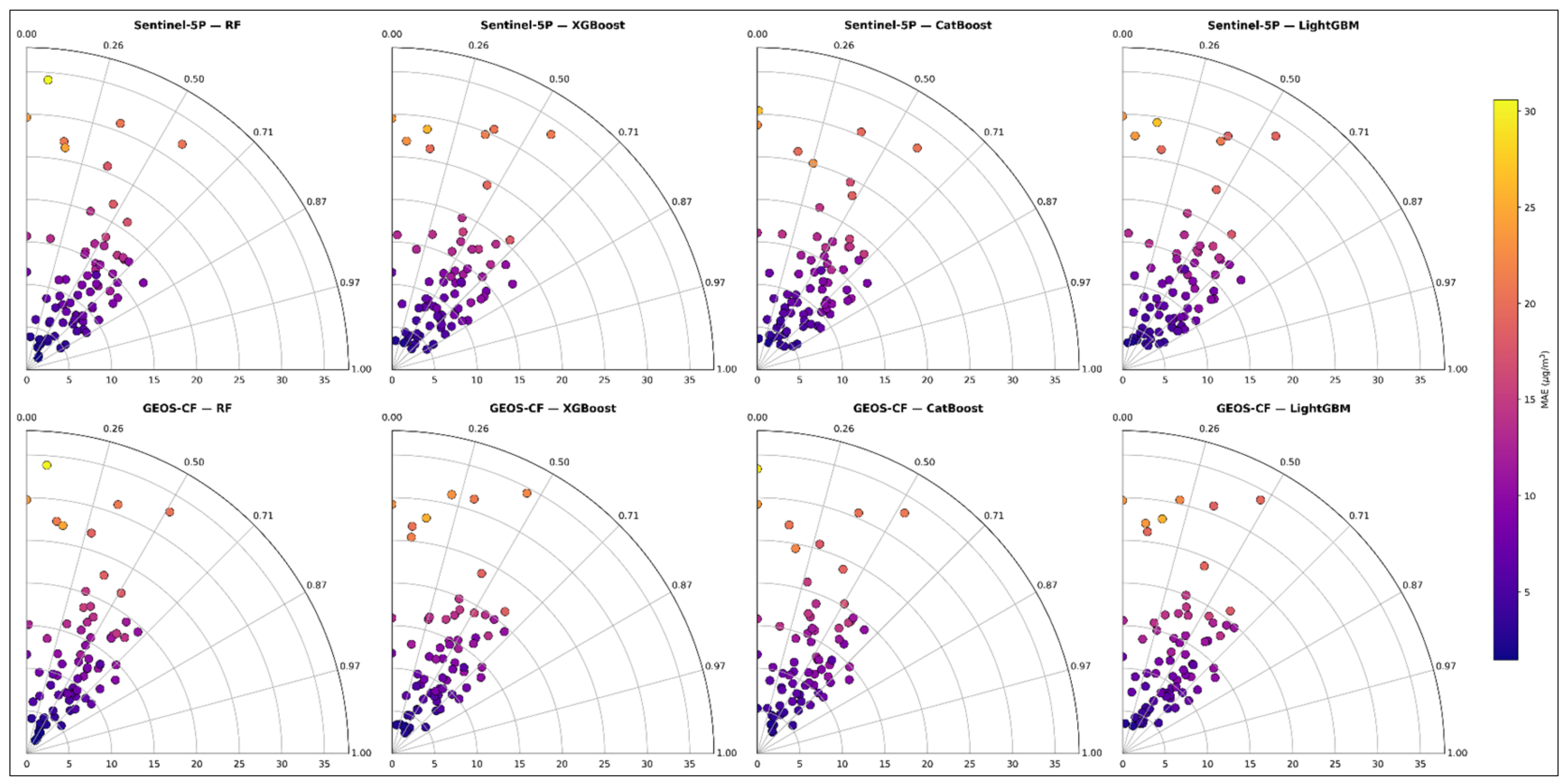
We further examined station-level errors for S5P-CatBoost, finding marked spatial heterogeneities in prediction accuracy (Figure 6). Across the 74 test stations, R ranged from −0.09 to 0.84 and RMSE from 3.43 to 32.11 µg/m³. The highest errors were concentrated at a small number of stations in Istanbul: Uskudar MTHM (RMSE = 32.11 µg/m³), Kagithane (30.47), Catladikapi (30.40), and Selimiye (28.74). Selimiye and Sultangazi MTHM recorded negative R values (−0.092 and −0.047, respectively), and Catladikapi and Kirklareli showed near-zero values (0.005 and 0.043, respectively). The strongest agreements were observed at Istanbul–Sancaktepe (R = 0.84, RMSE = 5.56 µg/m³), Istanbul–Maslak (R = 0.84, RMSE = 8.90), Bilecik–Bozuyuk (R = 0.84, RMSE = 4.96), and Istanbul–Bagcilar (R = 0.81, RMSE = 8.77).

4.3. Spatial Cross-Validation Results

Performance under spatial cross-validation was substantially lower than under the temporal split. For the S5P feature set, LOSO and LOPO yielded mean R values of 0.494 and 0.501, respectively, well below the R = 0.706 obtained under the temporal split (

Table 5. Cross-validation strategy comparison for the S5P-CatBoost configuration.

CV Strategy	R	R2	RMSE (µg/m3)	MAE (µg/m3)
Random (70/10/20)	0.844	0.712	11.68	7.54
Temporal (2024 test)	0.706	0.498	14.31	9.51
LOSO (74-fold)	0.494	0.244	15.14	11.67
LOPO (11-fold)	0.501	0.251	12.77	8.84

). The S5P advantage over GEOS-CF persisted under both strategies (LOSO ΔR = +0.058; LOPO ΔR = +0.045), exceeding the +0.028 gap observed under temporal split.

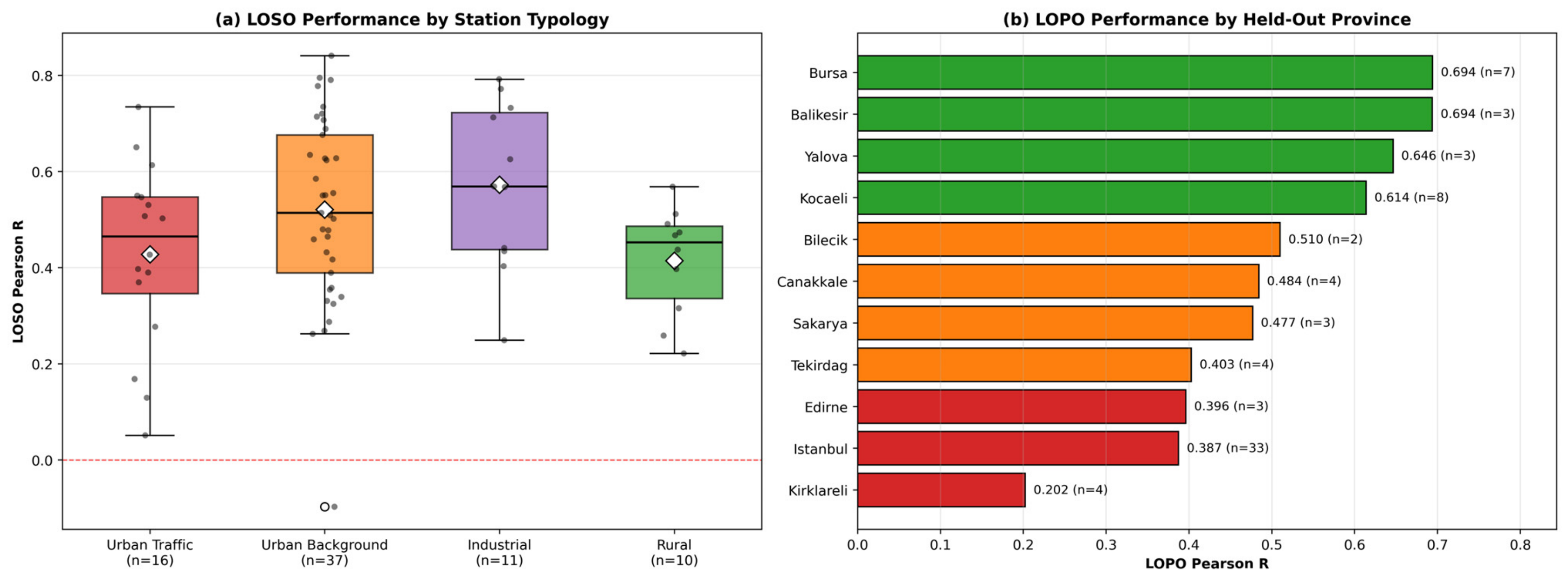
LOSO performance varied with station typology (

Table 6. LOSO performance by station typology (S5P-CatBoost).

Typology	n	R	RMSE (µg/m3)	MAE (µg/m3)	Bias (µg/m3)	Observed Mean (µg/m3)
Industrial	11	0.572	14.57	10.13	+0.75	16.94
Urban Background	37	0.521	13.50	10.84	+3.82	19.05
Urban Traffic	16	0.428	23.96	18.61	−9.30	40.92
Rural	10	0.414	7.72	5.31	+1.96	6.99

). Industrial stations achieved the highest mean R (0.572), followed by Urban Background (0.521), Urban Traffic (0.428), and Rural (0.414). Rural stations showed the lowest absolute errors (RMSE = 7.72, MAE = 5.31 µg/m³), while Urban Traffic stations exhibited the highest absolute errors (RMSE = 23.96 µg/m³) and the largest negative bias (−9.30 µg/m³).

LOPO performance varied substantially by held-out province (Figure 7). Bursa (R = 0.694), Balikesir (R = 0.694), and Yalova (R = 0.646) achieved the strongest transfer, while the lowest performance was observed for Kirklareli (R = 0.202) and Istanbul (R = 0.387, RMSE = 23.68 µg/m³).

4.4. SHAP Analysis

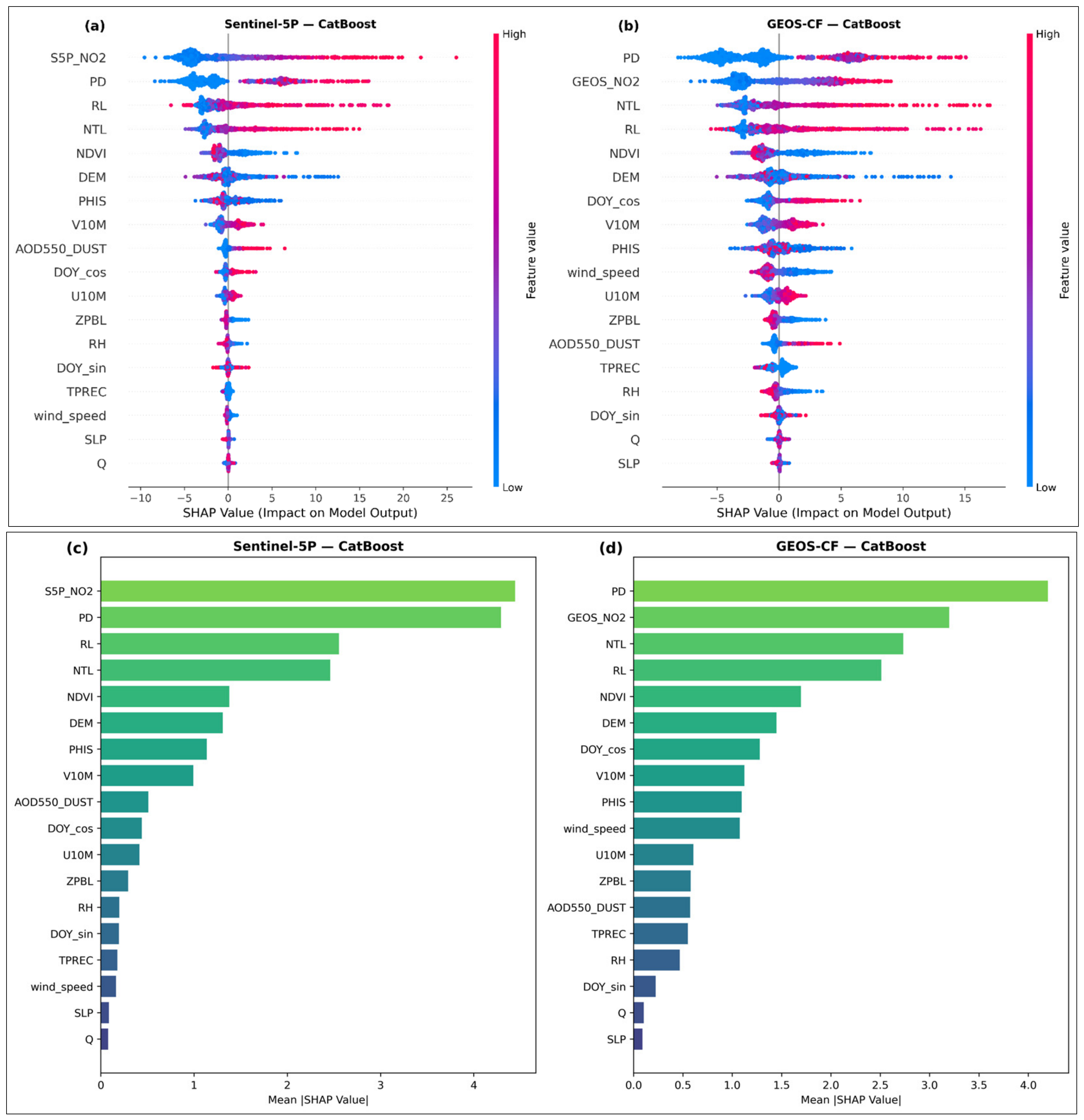
As outlined in Section 4.2, we applied SHAP analysis to the best-performing CatBoost models from both feature sets. The resulting summary plots and feature importance rankings are shown in Figure 8, where the horizontal axis indicates the SHAP value of each feature, the vertical axis lists features in descending order of importance, and the color scale runs from blue (low feature values) to pink (high feature values).

In the S5P summary plot (Figure 8a), S5P_NO₂ ranks first with the widest SHAP spread (mean |SHAP| = 4.44); high VCD values cluster in the positive SHAP region, whereas low VCD values cluster in the negative region. PD (4.29), RL (2.55), and NTL (2.46) ranked immediately below and share the same directional pattern of high values corresponding to positive SHAP values, reflecting the expected link between anthropogenic activity and NO₂ predictions. The reverse is observed for NDVI at the fifth rank (1.38); i.e., densely vegetated areas cluster in the negative SHAP region. DEM (1.31) shows a similar pattern, PHIS ranks seventh, and the remaining meteorological features rank lower, with narrower SHAP distributions. The GEOS-CF summary plot (Figure 8b) reveals some differences. PD ranks first (4.20), followed by GEOS_NO₂ (3.20) in second. NTL (2.73) and RL (2.51) rank third and fourth, and NDVI (1.70) remains fifth. DOY_cos ranks notably higher than in the S5P model (seventh versus tenth) and V10M, wind_speed, and ZPBL showed wider SHAP distributions. The top four features (NO₂ VCD, PD, RL, NTL) are shared across both models, though their ordering differs; NDVI and DEM rank fifth and sixth in both. Since these rankings do not reveal how feature values translate into SHAP values, dependence plots were generated for the four most influential S5P-CatBoost features (Figure 9).

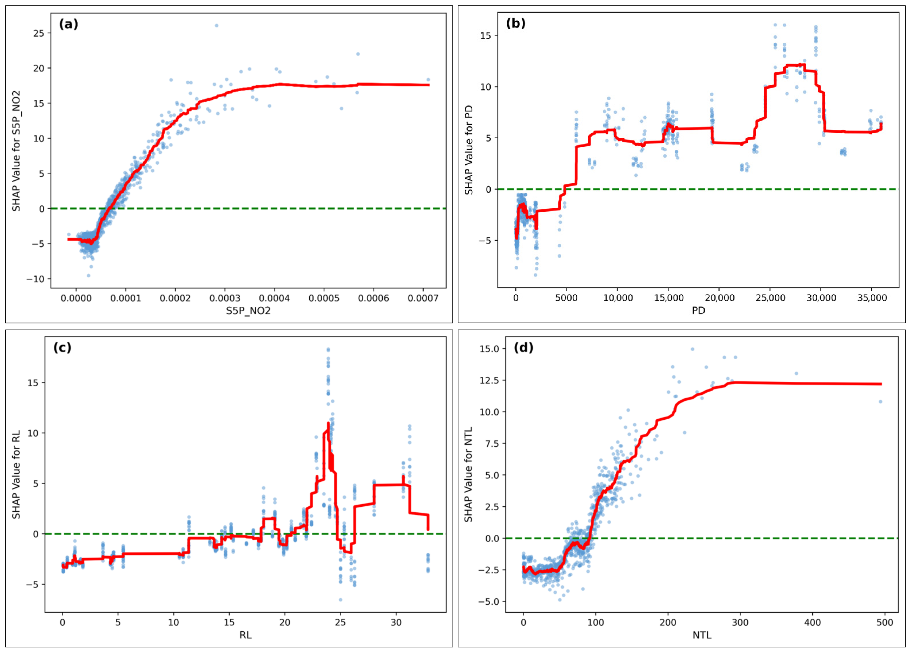
The S5P_NO₂ dependence plot (Figure 9a) shows the trend remaining flat at approximately −5 at low VCDs, rising steeply from ~0.00007 mol/m², and leveling off into a saturation plateau at +15 to +18 above ~0.0004 mol/m². In the PD plot (Figure 9b), the trend line remains negative (−5 to −3) up to ~5000 persons/km², whereupon it crosses zero, increases to ~+12 near 26,000–28,000 persons/km², and declines at the highest densities. The considerable scatter at high PD values indicates that PD alone does not fully determine local NO₂ levels. The RL and NTL plots (Figure 9c,d) both exhibit threshold-driven responses. RL crosses zero at ~18 km per grid cell and rises to +5 to +11 at higher road densities; however, the pronounced scatter and multiple zero-crossings at the upper end suggest that the relationship is influenced by local factors that are not captured by RL alone. In the NTL plot, a sigmoidal rise from near zero to ~+12 occurs between 65 and 260, indicating that NTL has its strongest marginal effect in the rural-to-urban light transition. To complement the static feature rankings, we examined their temporal stability. Yearly SHAP rankings were computed by applying the S5P-CatBoost model to subsamples from each year (2019–2024). The pairwise Spearman rank correlation between years averaged ρ = 0.992 (range 0.981–1.000), and the correlation between the training period mean (2019–2022) and the test year (2024) was ρ = 0.995. The same four predictors (S5P_NO₂, PD, RL, and NTL) appeared in the top 5 across all six years. PD ranked first in 2019–2020 and S5P_NO₂ from 2021 onward. The Pearson correlation between PD and S5P_NO₂ was R = 0.270, well below the 0.8 multicollinearity threshold, indicating that they provide complementary information. As an additional check on inter-period stability, the principal meteorological and column predictors were compared between the training (2019–2022) and test (2024) periods: ZPBL, wind_speed, and S5P_NO₂ differed by less than 5% in their mean values, RH and Q shifted by 7–10%, and AOD550_DUST showed the largest shift (+28%); the four highest-ranked predictors thus remained distributionally stable across periods.

4.5. Seasonal and Annual NO₂ Mapping

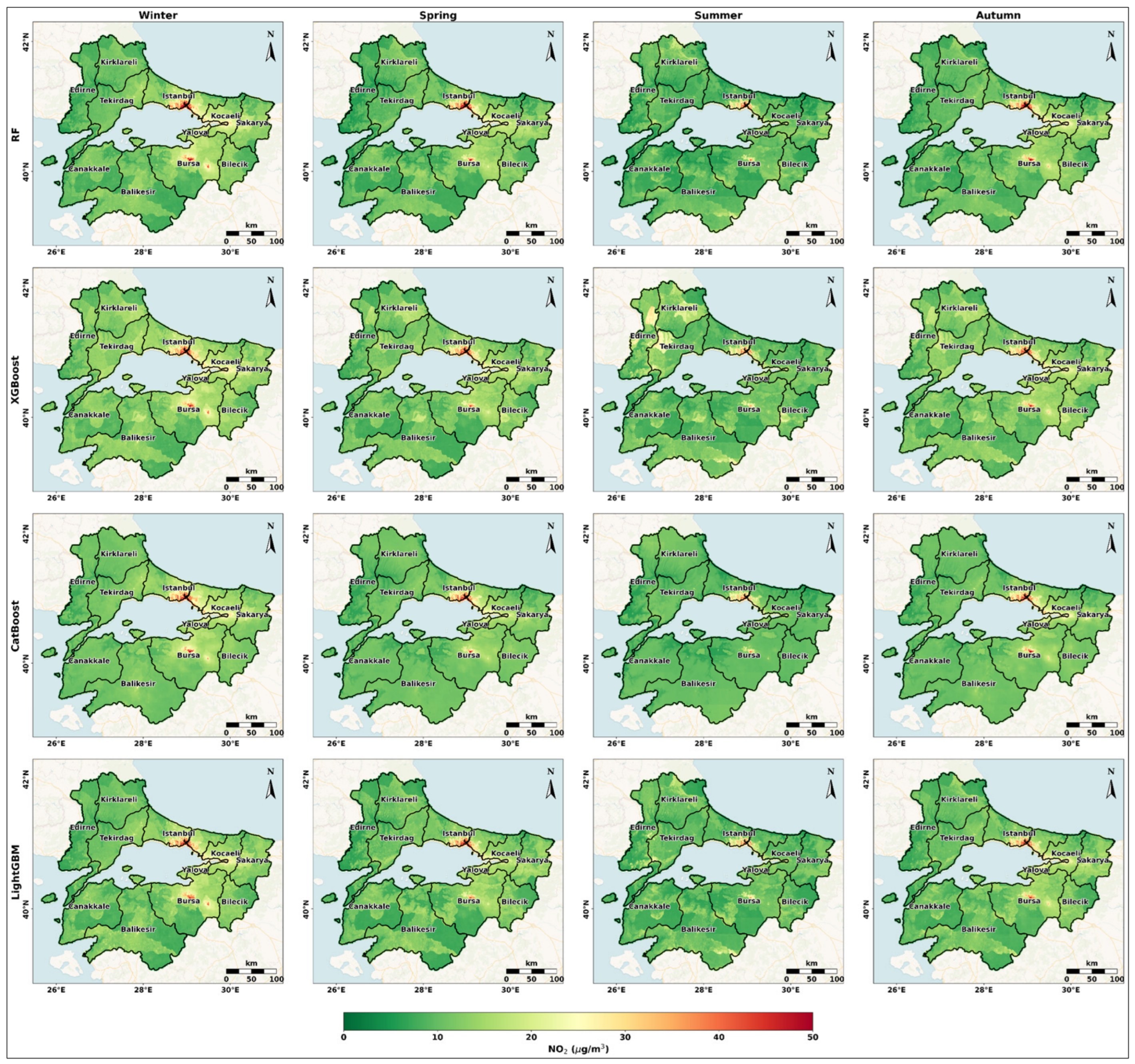
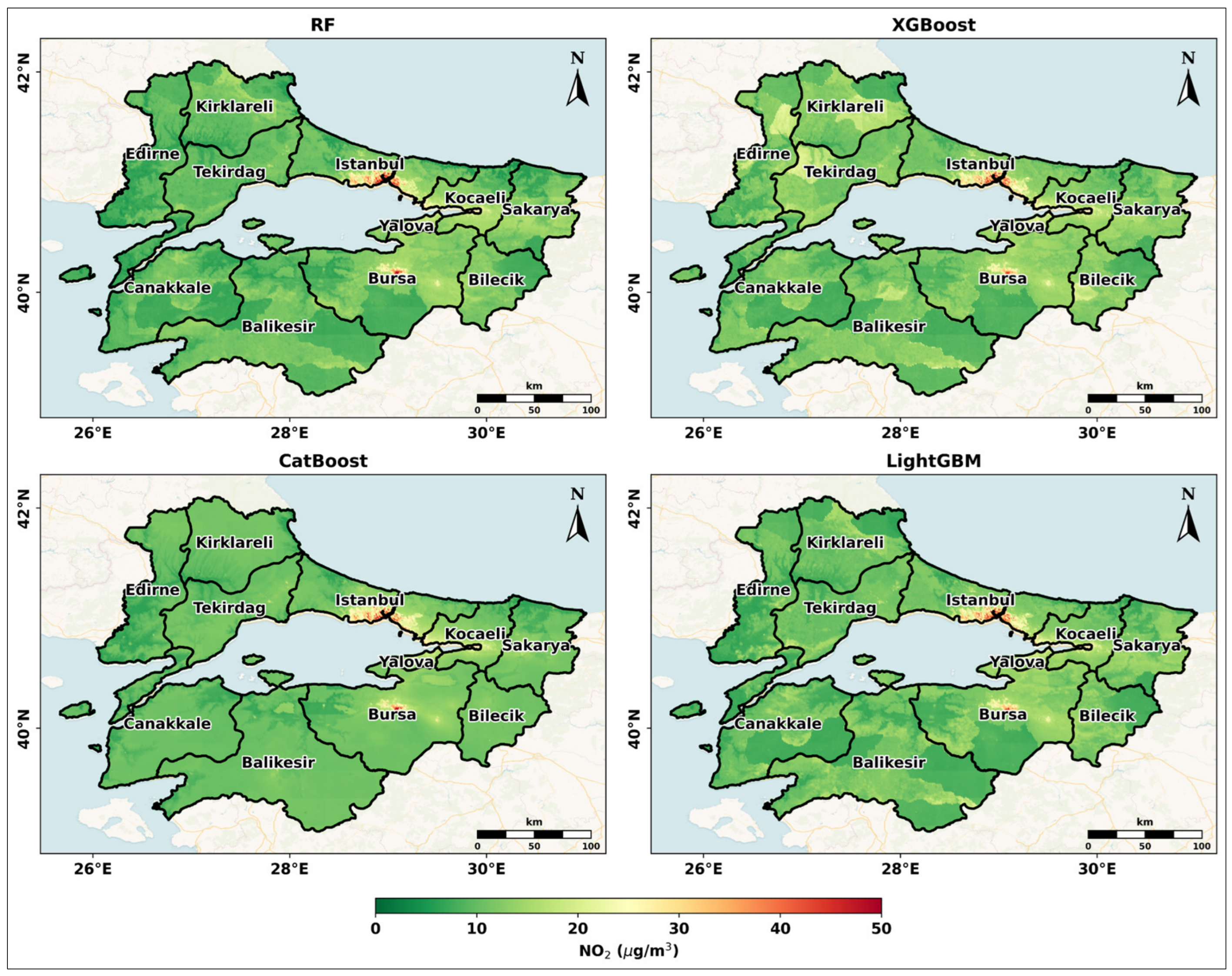
The temporally split models generated daily NO₂ predictions for 2024 on a 0.01° grid across the Marmara Region. These daily predictions were aggregated into seasonal and annual mean concentration maps. Seasonal NO₂ maps for all four models under the S5P feature set are shown in Figure 10.

Figure 10 highlights differences in spatial texture and seasonal behavior across the four S5P-based models. In the winter panels, high-concentration areas exceeding 40 µg/m³ are clearly visible along the Istanbul–Kocaeli corridor and in parts of Bursa, whereas the rest of the region retains low to moderate levels. From winter to summer, a progressive shift toward uniformly low concentrations occurs as most of the study area falls below 20 µg/m³; the autumn panels then show a partial return of moderate-to-high values. All four models identify the Istanbul–Kocaeli–Bursa industrial corridor as the dominant high-concentration area in every panel, the overall seasonal gradient of which is visually indistinguishable between models. XGBoost maps exhibit noticeably noisier spatial fields, with small-scale pixelation particularly prominent in winter and spring. CatBoost, by contrast, produces the smoothest and most spatially continuous outputs across all seasons; RF and LightGBM fall between these two extremes. The spring and autumn columns are also nearly identical with spatial distributions remaining indistinguishable despite similar regional means.

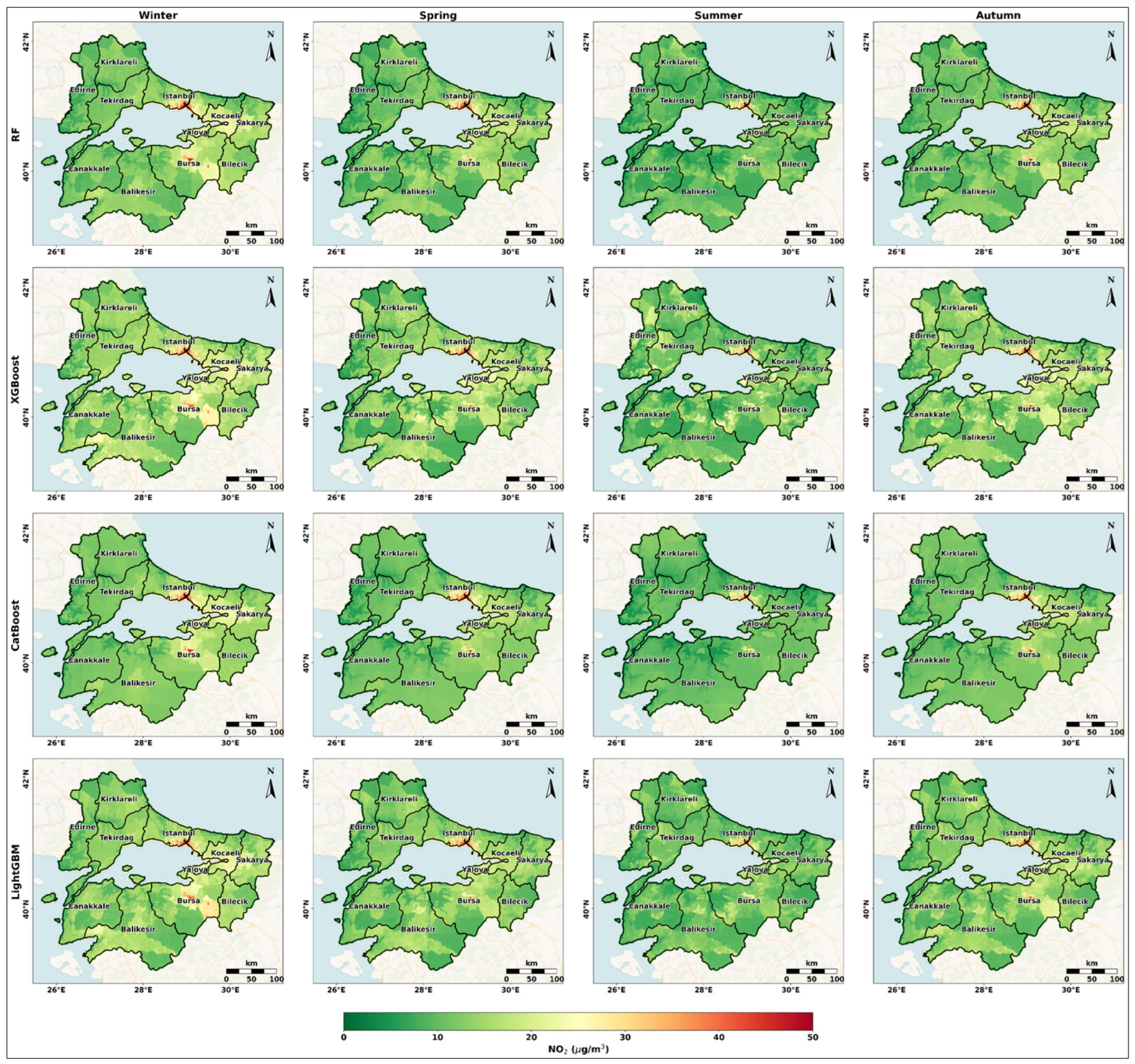
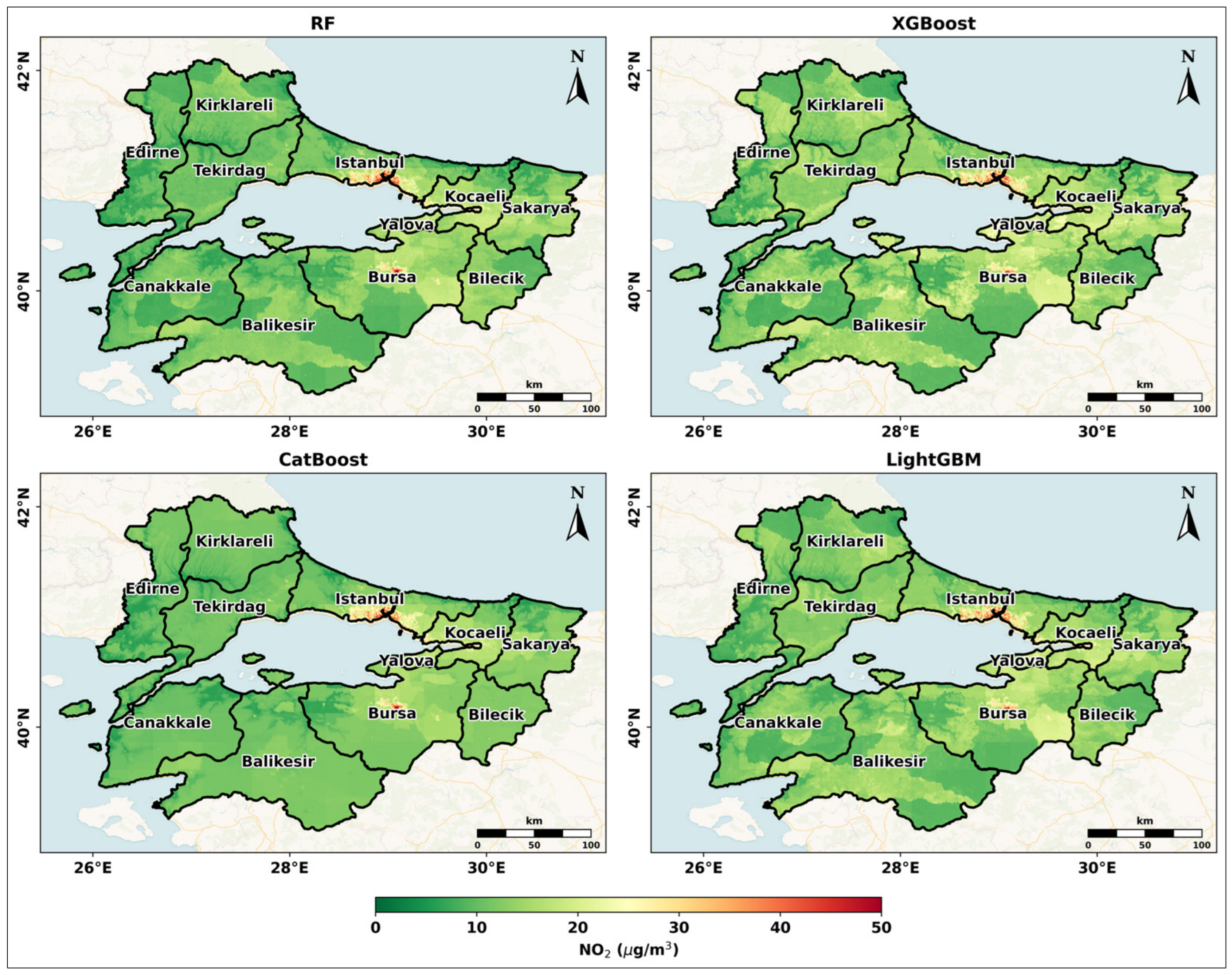
The spatial structures of GEOS-CF-based seasonal maps (Figure 11) closely resemble their S5P counterparts. Transitions between adjacent grid cells, however, appear markedly blockier; this is a direct consequence of the coarser native resolution of the GEOS-CF input. XGBoost again produces the noisiest outputs, whereas the other three models yield more spatially homogeneous fields.

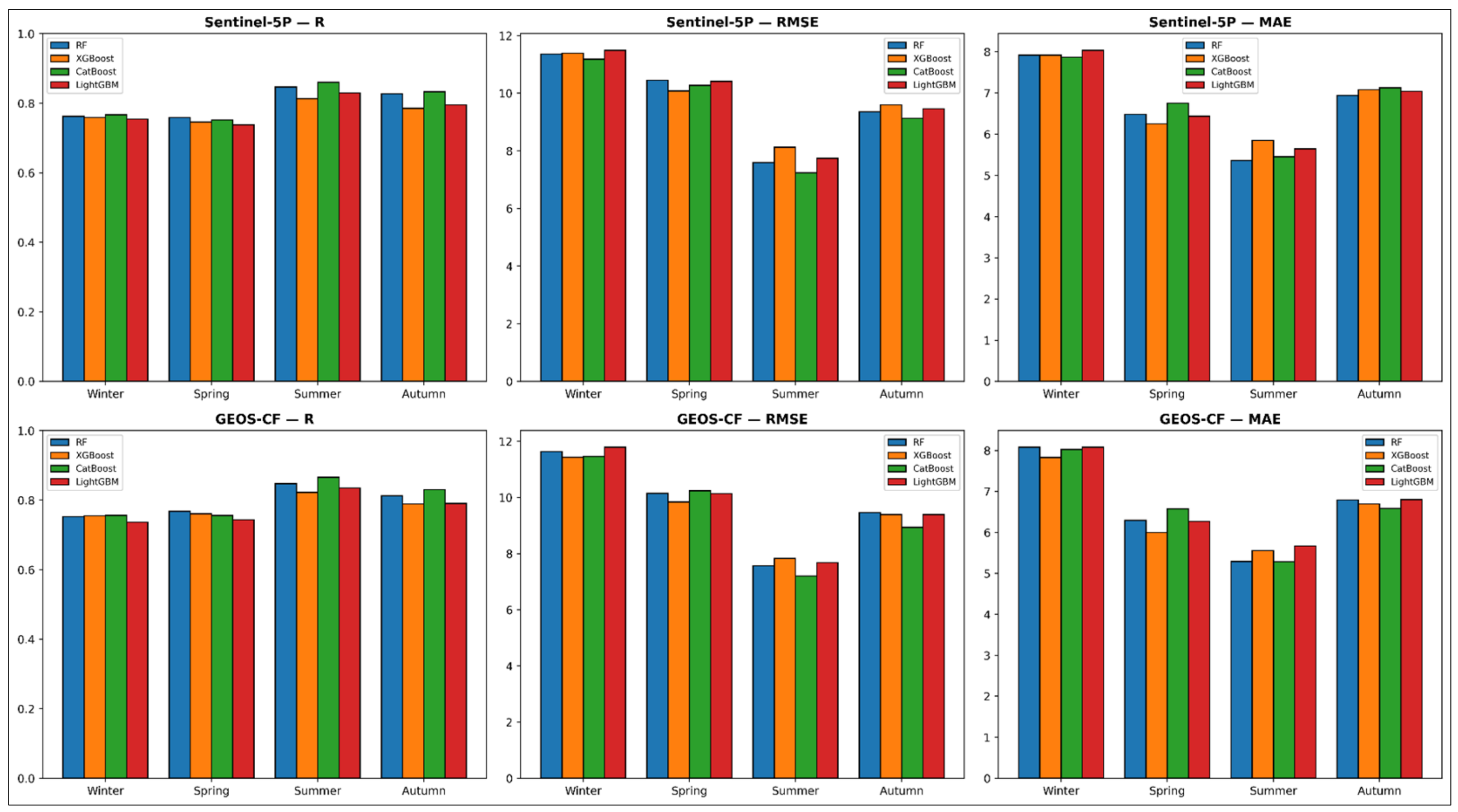
To assess whether these spatial patterns are reflected in quantitative performance, we compared station-averaged seasonal predictions against observations for the test year (Figure 12). Pronounced performance differences emerged across seasons: summer yielded the highest R values (0.81–0.87 across all configurations) and the lowest RMSE (7.20–8.13 µg/m³), whereas winter produced the lowest R (0.74–0.77) and highest RMSE (11.18–11.79 µg/m³). Autumn was similar to summer (R = 0.79–0.83, RMSE = 8.93–9.59 µg/m³). Spring matched winter in correlation (R = 0.74–0.77) but with lower errors (RMSE = 9.84–10.45 µg/m³). The ranking summer > autumn > spring ≈ winter held across all eight model-feature set combinations examined. CatBoost achieved both the highest summer R (0.86 for S5P, 0.87 for GEOS-CF) and winter R (0.77 for S5P, 0.76 for GEOS-CF). Although S5P-based models outperformed GEOS-CF in overall test metrics (Section 4.2), this advantage did not persist uniformly across seasons; in spring and summer, GEOS-CF models achieved comparable or marginally higher R values.

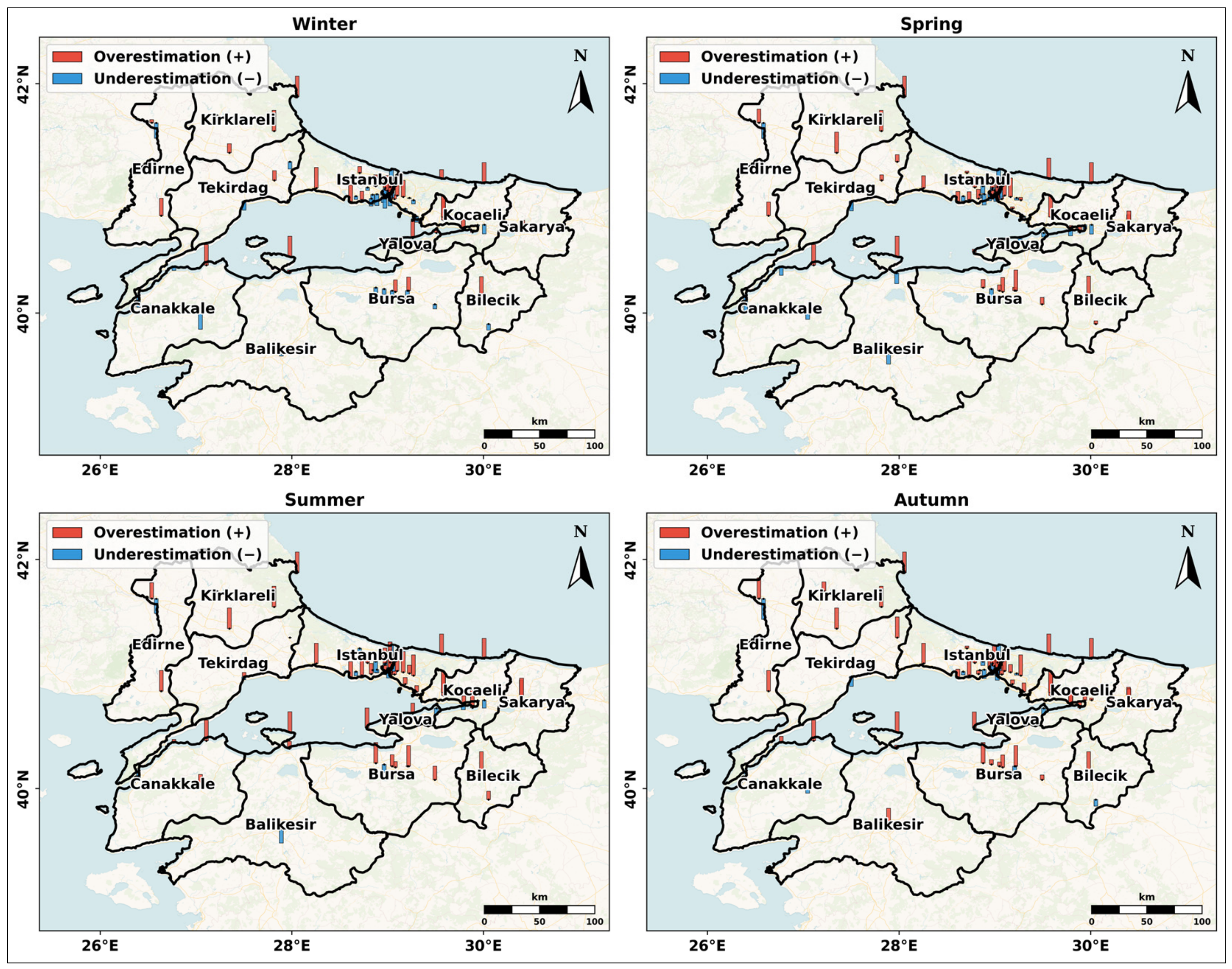
Seasonal relative error maps for S5P-CatBoost (Figure 13) reveal systematic patterns in model bias. In winter, overestimation and underestimation were largely balanced across stations (median relative error: −0.1%), retaining a wide interquartile range (−17% to +34%). Summer and autumn showed a clear overestimation tendency: 72% and 74% of stations overestimated, with median relative errors of 26% and 23%, respectively. Spring showed an intermediate position, with 60% of stations overestimated and a median value of 9%. The largest positive relative errors were concentrated at low-concentration peripheral stations, where even small absolute biases translate into high percentage deviations. In contrast, underestimation was distributed across urban and non-urban stations, with no single province dominating. Following seasonal analyses, we averaged daily predictions throughout the full year to produce annual mean NO₂ maps across the region (Figure 14). S5P-based annual means ranged from 10.93 µg/m³ (RF) to 12.34 µg/m³ (XGBoost), with CatBoost yielding a regional mean of 11.20 µg/m³. RF and LightGBM showed very similar spatial structures, while CatBoost displayed noticeably smoother concentration fields. The Istanbul–Kocaeli–Bursa corridor emerges as the dominant high-concentration zone, with values locally exceeding 30 µg/m³ in central Istanbul and the Bursa urban core. Away from this dense core, concentrations follow a clear radial gradient, declining progressively toward the surrounding provinces. The rural fringes, particularly in the Trakya subregion (Edirne, Kirklareli, and Tekirdag) and parts of southern Balikesir, form the cleanest areas on all four maps, whereas Yalova, despite its small area, exhibits notably elevated values relative to its neighbors.

GEOS-CF-based annual mean maps (Figure 15) reproduce a similar spatial pattern. Annual means ranged from 12.02 µg/m³ (RF and CatBoost) to 13.66 µg/m³ (XGBoost), with a comparable inter-model spread for both feature sets (1.64 µg/m³ for GEOS-CF vs. 1.41 µg/m³ for S5P). A grid-level comparison, however, revealed that GEOS-CF predictions systematically exceeded their S5P counterparts across all seasons and models, with the most pronounced offsets concentrated in the Istanbul–Kocaeli urban core. This pattern is consistent with the spatial resolution difference between the two column sources propagating directly into the predictions.

To quantify predictive uncertainty, we performed 1000 bootstrap iterations of the S5P-CatBoost configuration on the test set, yielding R = 0.702 (95% CI: 0.698–0.707), RMSE = 14.61 µg/m³ (95% CI: 14.47–14.75), and MAE = 9.46 µg/m³ (95% CI: 9.36–9.54). Because resampling with replacement leaves approximately 37% of unique observations out of each iteration on average, the bootstrap mean RMSE (14.61) slightly exceeds the test-set value in Table 4 (14.31). Total prediction intervals, combining bootstrap variance with the standard deviation of training residuals (9.15 µg/m³), achieved 85.8% empirical coverage at the 95% nominal level. The empirical coverage below the nominal level indicates mild underdispersion of the prediction intervals, primarily driven by the high-concentration regime (

Table 7. Test-set bias decomposition by observed NO₂ concentration range (S5P-CatBoost, temporal split).

Concentration Range (µg/m3)	n	% of Test	Mean Observed (µg/m3)	Mean Predicted (µg/m3)	Mean Bias (µg/m3)
[0, 10)	4849	38.3	5.20	12.05	+6.86
[10, 25)	4145	32.8	16.56	21.33	+4.77
[25, 50)	2616	20.7	34.92	31.89	−3.04
[50, 75)	772	6.1	60.08	44.07	−16.01
[75, 100)	193	1.5	83.78	56.43	−27.34
[100, 150)	64	0.5	117.96	60.90	−57.06
[150, 300)	17	0.1	179.63	56.24	−123.39

); within the bulk of the distribution (≤50 µg/m³, covering 91.8% of test observations), coverage remained close to the nominal level. Both uncertainty and bias varied systematically with concentration level. Coverage decreased with concentration: over 90% in 0–25 µg/m³, 79.1% in 25–50, 53.2% in 50–75, and 9.9% above 100 µg/m³. Mean bias followed a complementary pattern: modest overestimation in the lower bands (+6.86 µg/m³ for ≤10 and +4.77 µg/m³ for 10–25 µg/m³) transitioning to progressive underestimation above 50 µg/m³, reaching −57.06 µg/m³ in 100–150 and −123.39 µg/m³ in 150–300 µg/m³, where the sparsely sampled tail of the training distribution limits the model’s ability to extrapolate.

4.6. WHO AQG Assessment and Population Exposure

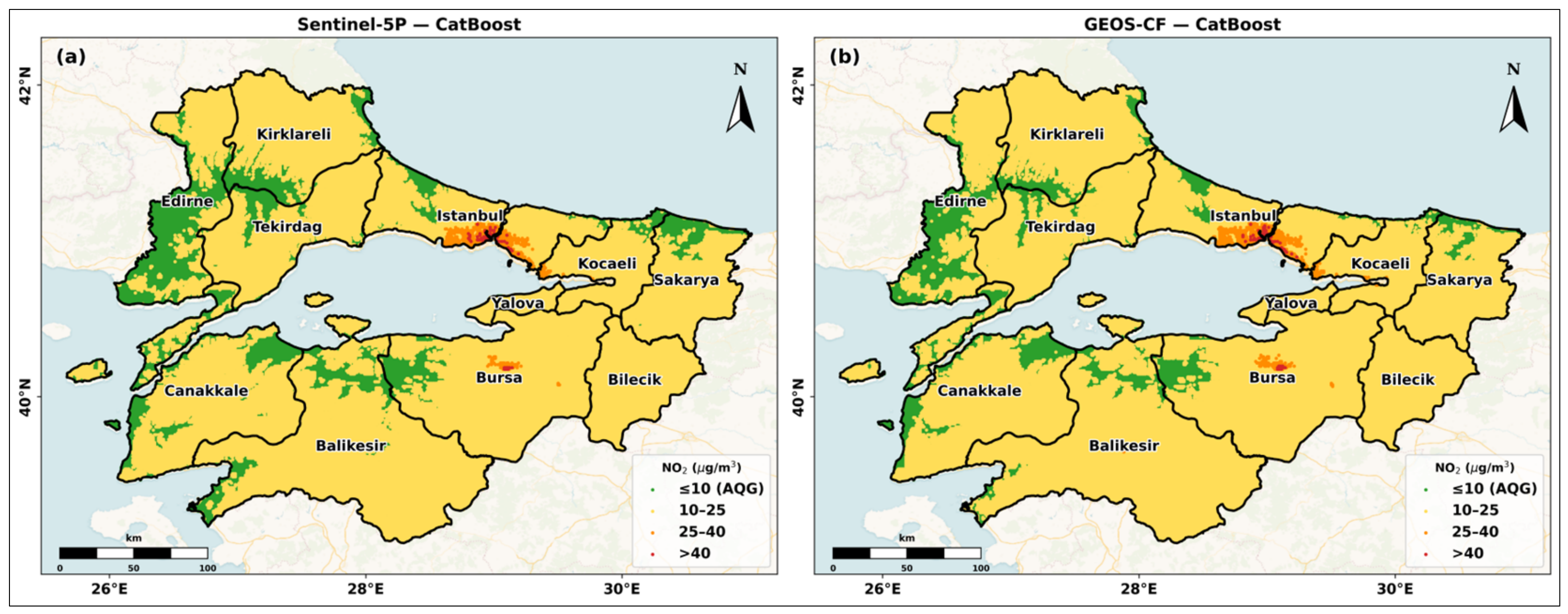
We evaluated the annual mean NO₂ concentration fields from Section 4.5 against WHO revised AQG levels [8], i.e., an annual mean of 10 µg/m³ and a 24 h mean of 25 µg/m³. Figure 16 presents the spatial distribution of annual mean NO₂ relative to the WHO annual AQG for the best-performing models from each feature set (S5P-CatBoost and GEOS-CF-CatBoost).

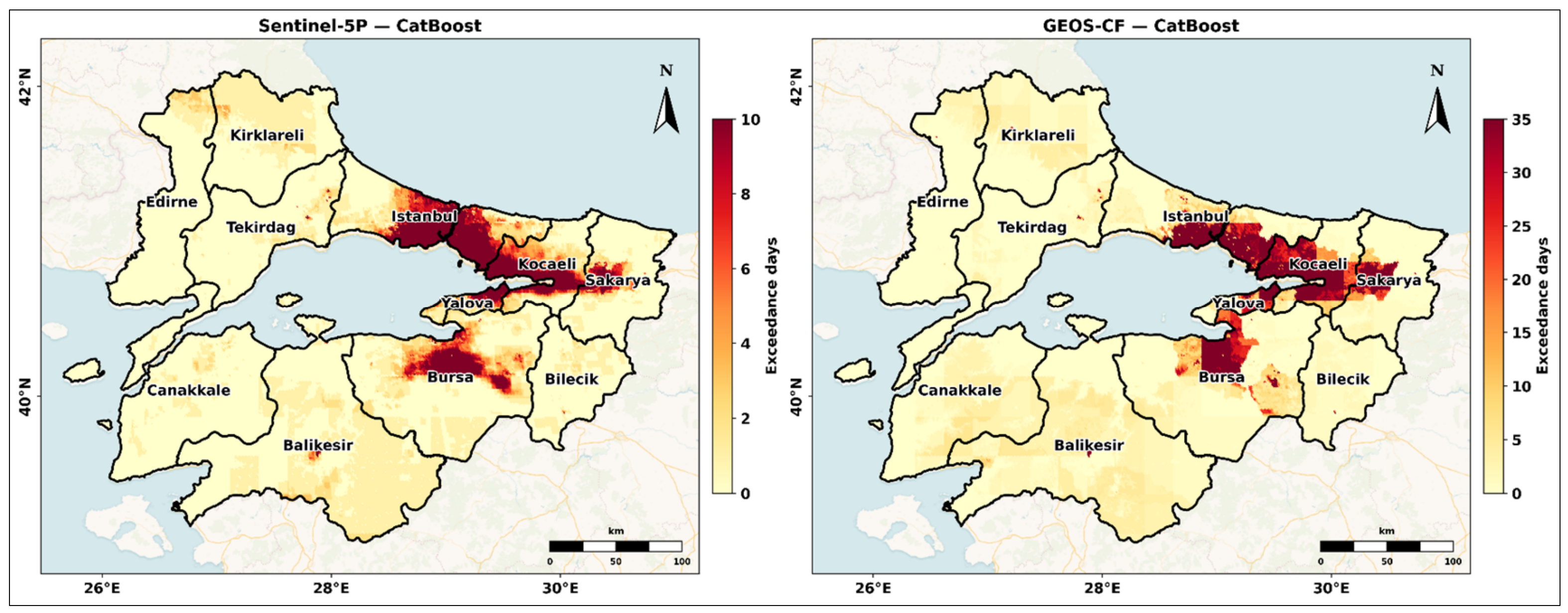
In the S5P-CatBoost map (Figure 16a), 81.1% of grid cells exceed the annual AQG of 10 µg/m³, with only scattered areas along the periphery falling below this threshold. The 10–25 µg/m³ category forms the dominant class, covering most of the region; the 25–40 µg/m³ range is concentrated in central Istanbul, with smaller clusters in Bursa and Kocaeli; and the >40 µg/m³ class appears only in a small number of grid cells at the urban core. AQG-compliant areas (≤10 µg/m³) are confined to Edirne, Kirklareli, parts of Canakkale and Balikesir, and higher-elevation zones in the south; Edirne exhibits the most extensive compliant coverage among all provinces. The GEOS-CF-CatBoost map (Figure 16b) shows the same spatial structure but contains a noticeably smaller compliant area and a wider moderate-concentration zone extending into the periphery, confirming a broader extent of AQG exceedance. To assess short-term exposure alongside the annual average, we mapped the number of days exceeding the 24 h AQG in Figure 17 for both CatBoost configurations.

In the S5P-CatBoost map, a substantial portion of the region experienced at least one exceedance day, with the highest counts concentrated along the Istanbul–Kocaeli corridor and in parts of Bursa; the region-wide mean was 3.0 days, with a maximum of 203 days. Despite its small area, Yalova exhibited daily exceedances across nearly its entire extent. In contrast, the western provinces of Edirne and Canakkale remained largely free of daily exceedances. The GEOS-CF-CatBoost model revealed a wider spatial extent of daily exceedances (56.0% of grid cells) with a mean of 7.2 days and a maximum of 365 days.

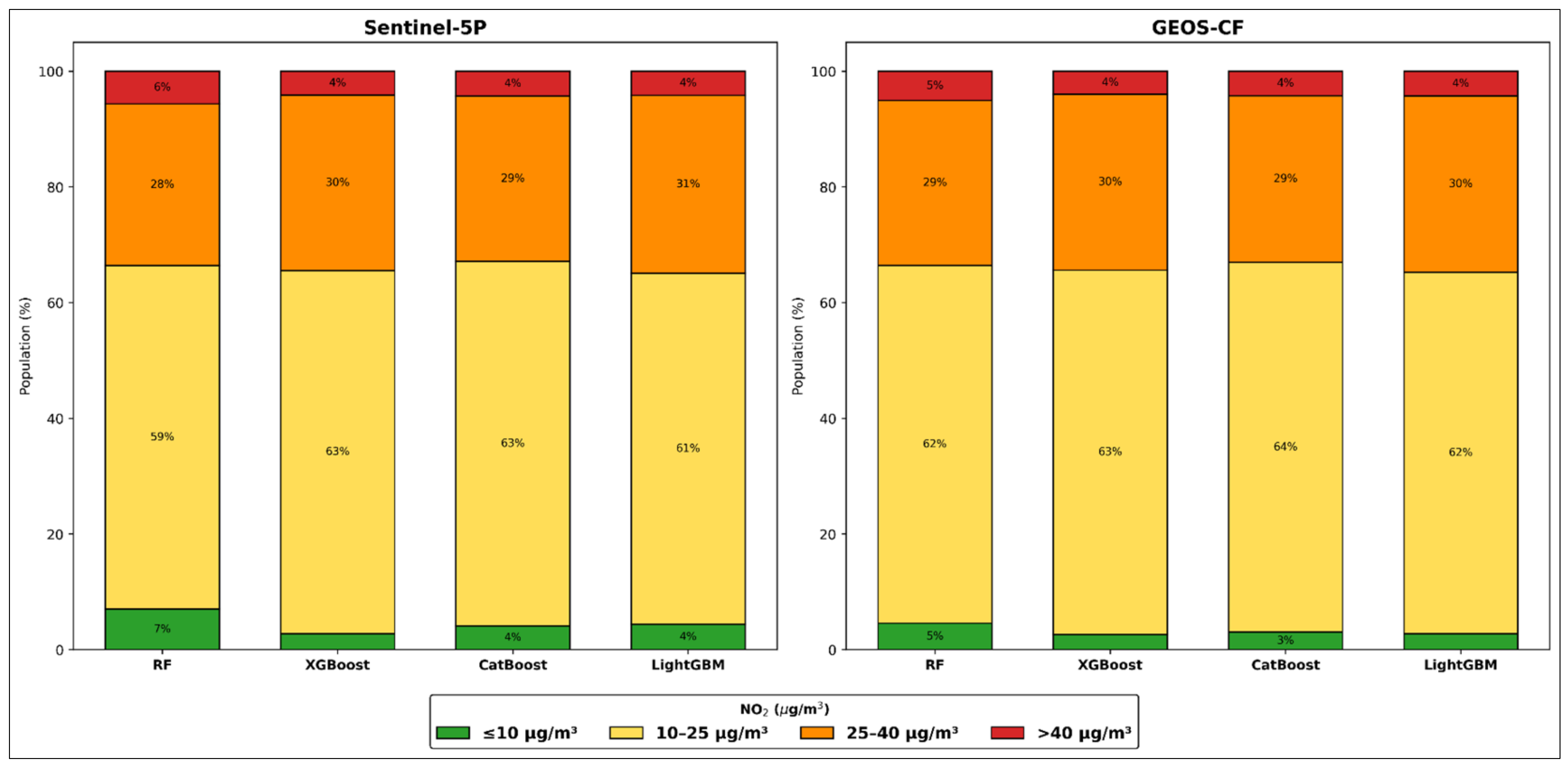
We also computed population-weighted annual mean NO₂ for each model configuration (Figure 18). Across all eight configurations, the population-weighted mean substantially exceeded the simple spatial mean: unweighted averages ranged from 10.93 to 13.66 µg/m³, whereas population-weighted values rose to 21.04–22.30 µg/m³. For S5P-CatBoost, the population-weighted annual mean was 21.08 µg/m³, approximately twice the WHO annual AQG. Only 4.1% of the region’s 26.74 million inhabitants resided in areas meeting the AQG; the remaining 95.9% were exposed above the threshold, with 63.0% falling in the 10–25 µg/m³ range, 28.6% in the 25–40 µg/m³ range, and 4.3% above 40 µg/m³.

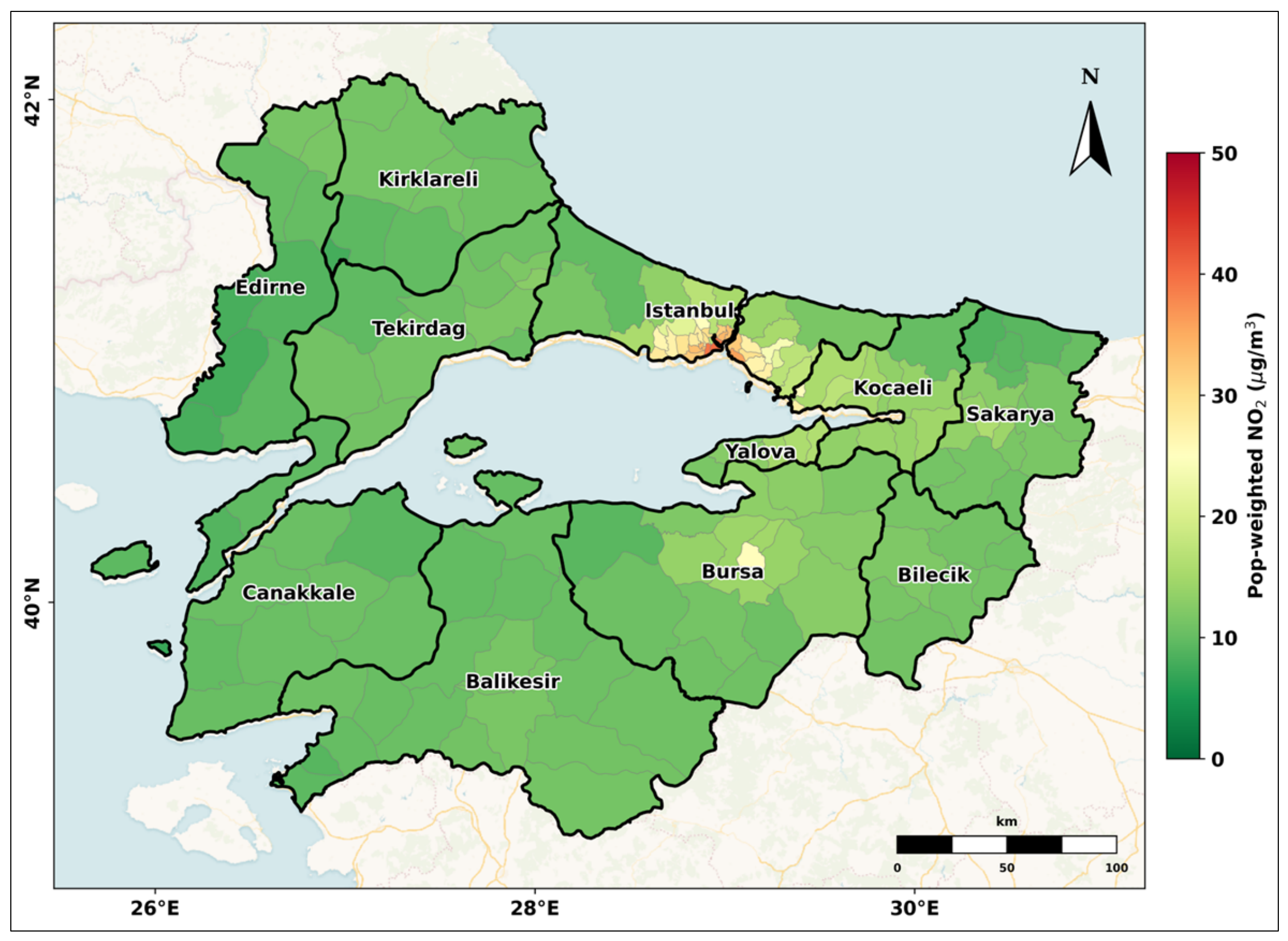
Population-weighted exposure followed the same seasonal cycle identified in Section 4.5: winter recorded the highest value (24.58 µg/m³), followed by spring (22.70 µg/m³), autumn (22.40 µg/m³), and summer (18.11 µg/m³). Even in summer, when the lowest concentrations were observed, 83.1% of the population was exposed to levels exceeding 10 µg/m³. In winter, this rose to 98.2%, and the proportion exposed to concentrations above 25 µg/m³ reached 45.4% (36.3% in the 25–40 range and 9.2% above 40 µg/m³). Beyond the region-wide assessment, the district-level map (Figure 19) reveals a marked spatial contrast. Across the 158 districts examined, the population-weighted annual mean NO₂ ranged from 7.18 µg/m³ (Bozcaada, Canakkale) to 39.91 µg/m³ (Fatih, Istanbul). The central and eastern districts of Istanbul appear in the highest-concentration class, whereas the western rural districts fall into the low-concentration range, producing a pronounced intra-urban gradient spanning more than 30 µg/m³ within a single province. The 15 districts with the highest exposure are located in Istanbul, including Fatih (39.91), Zeytinburnu (39.13), and Beyoglu (38.81 µg/m³), all of which recorded 100% grid-cell exceedance of the annual AQG. Outside Istanbul, the highest-exposed districts were Darica in Kocaeli (27.47 µg/m³) and Yildirim in Bursa (25.31 µg/m³). At the opposite extreme, the lowest-concentration districts on the map occur in Edirne (Enez: 8.18, Ipsala: 7.93 µg/m³) and Kirklareli (Pehlivankoy: 7.97 µg/m³). Of the 158 districts, 132 had population-weighted annual means exceeding 10 µg/m³.

5. Discussion

This study estimated ground-level NO₂ concentrations across the Marmara Region by combining S5P and GEOS-CF tropospheric NO₂ VCD data with meteorological, topographic, land-use, and socioeconomic predictors through four tree-based ensemble algorithms. The best-performing temporal split configuration (S5P-CatBoost) represents an improvement over an Istanbul-only framework [47] in both correlation and error magnitude. The value of R² remains lower than values previously reported [11] under spatial and temporal cross-validation over East Asia, although differences between region, station density, and pollutant variability complicate direct comparison. For MAE, the result (9.51 µg/m³) is somewhat higher than the 7.77 µg/m³ reported by [36] for Europe, where station density is considerably greater. Studies relying on random cross-validation consistently report higher metrics, e.g., R² = 0.78 with RF in China [81] and R² = 0.93 under random and 0.71 under out-of-city cross-validation using a deep forest model [37]. A similar reduction was observed herein: random splitting yielded performance comparable to that reported by [81], which dropped substantially under a temporal split. A similar pattern has been reported for ground-level NO₂, with R² dropping from 0.89 under sample-based to 0.59 under area-based cross-validation [39].

The systematic difference between random and temporal splits reflects data leakage caused by spatiotemporal autocorrelation. The authors of [38] demonstrated ~48% RMSE inflation between random and spatial cross-validation in satellite-based PM_2.5 models, and [82] reported R² dropping from 0.53 to 0.14 under spatial cross-validation in tropical forest biomass mapping. The inflation was largest for XGBoost and LightGBM, consistent with [11]. Under the temporal split, the four models converged to nearly identical performance, indicating that feature quality rather than algorithm choice becomes the determining factor once autocorrelation is removed. The LOSO and LOPO analyses (Section 4.3) revealed an additional R reduction of ~0.21 beyond the temporal split, quantifying the cost of geographic transfer. Performance varied with station typology: Industrial (R = 0.572) and Urban Background (R = 0.521) sites achieved the highest transfer among the four typologies, while Urban Traffic stations exhibited systematic underestimation at high concentrations (bias = −9.30 µg/m³). Rural stations combined the lowest R (0.414) with the lowest absolute error (RMSE = 7.72 µg/m³), reflecting the limited dynamic range at low-concentration sites rather than model failure. Transfer to Istanbul (R = 0.387) and Kirklareli (R = 0.202) was substantially weaker. For Istanbul, this partly reflects that withholding the province removes 44% of the training observations; together, these results indicate that major urban areas and peripheral rural regions require local training data.

SHAP analysis identified the features with the largest mean absolute attribution to the CatBoost predictions. The satellite-derived NO₂ column ranked first, followed by PD, RL, and NTL intensity. These attribution patterns were then compared with the established literature on NO₂ emission and dispersion to assess their physical plausibility. This hierarchy aligns with [36], who identified TROPOMI NO₂ and VIIRS NTL as the top two predictors across Europe, and with [83], who showed that population, income, urban contiguity, and meteorology explained a substantial share of urban NO₂ variance across 83 cities. In the GEOS-CF model, NO₂ VCD ranked second as higher-resolution land-use proxies became more important, a shift also reported in Istanbul [47]. This reflects the coarser resolution of GEOS-CF (~0.25°), which limits spatial discrimination and shifts the explanatory weight onto higher-resolution land-use proxies. Dependence plots revealed nonlinear patterns consistent with prior SHAP-based studies [84,85]: a saturation plateau at high VCD values, a non-monotonic PD attribution profile peaking in the densely urbanized range and decreasing thereafter, and a sigmoidal NTL response across the rural-urban transition. NDVI contributed monotonically and negatively, consistent with reduced emission source density in vegetated areas [36]. Among these patterns, the VCD saturation plateau directly constrains prediction performance. With the training distribution providing little support beyond P95 = 67.6 µg/m³ and tree-based ensembles unable to extrapolate, the model’s response to VCD flattens rather than continuing to increase, producing the underestimation observed above 50 µg/m³. Predictive uncertainty followed the same pattern, with coverage falling below 10% above 100 µg/m³.

Seasonal model performance differed substantially: summer outperformed winter in both correlation and error magnitude, with RMSE decreasing by approximately one-third between the two seasons. This seasonal contrast is consistent with the longer atmospheric lifetime of NO_x in winter: lifetimes of 5.9 h have been reported in summer versus 21 h in winter over eastern China [86], implying that winter NO₂ accumulates over larger areas and introduces greater spatial variability that is harder to capture. A corresponding pattern has been documented at stations across the Marmara Region, with concentrations peaking in winter and declining to minima in summer [46]. In addition to atmospheric chemistry, the superior summer performance also reflects better TROPOMI data availability: 70–80% coverage has been reported over the climatically similar Iberian Peninsula in summer, dropping to 30–45% during cloudy months [21]. Overall, S5P-based models held a modest RMSE advantage over their GEOS-CF counterparts, attributable to the finer spatial resolution of TROPOMI; however, this gap narrowed or reversed at the seasonal level, with GEOS-CF achieving comparable or marginally higher correlation in spring and summer. GEOS-CF maps exhibited blockier spatial transitions, consistent with the limited ability of the system to resolve fine-scale features at its native resolution [23].

When evaluated against the WHO revised AQG, the region showed widespread exceedances: 81.1% of grid cells exceeded the annual threshold, and the population-weighted mean reached 2.1 times the recommended level, with only a small fraction of the population residing in compliant areas. At these exposure levels, the associated health burden is not negligible: a relative risk of RR = 1.02 per 10 µg/m³ has been reported for all-cause mortality [87], and it has been estimated that 4.0 million new pediatric asthma cases per year could be attributable to NO₂ globally [88]. District-level disparities were equally striking, spanning a more than fivefold range from the cleanest island districts to the most burdened central Istanbul neighborhoods. This pattern aligns with the persistent urban exposure gradients documented across Europe [89]. Even in summer, the majority of residents remained above the annual guideline, whereas winter exposure placed nearly half the population beyond the 24 h threshold.

This study has several limitations, beginning with the satellite input: TROPOMI’s single daytime overpass at ~13:30 local time cannot resolve the morning and nighttime NO₂ peaks [20], with the framework therefore operating at daily resolution; cloud contamination further limits winter availability, introducing a potential fair-weather bias; and tropospheric NO₂ VCD uncertainties of ~40% have been estimated over polluted scenes [90]. On the modeling side, vertical mixing dynamics, including thermal inversion episodes, are represented only indirectly through the planetary boundary layer height (ZPBL) predictor, and explicit coupling with chemical transport model outputs is not implemented in the present framework. Spatial generalization presents a further set of constraints (Section 4.3), partly reflecting the underlying sparsity of the ground station network: with NO₂ exhibiting strong fine-scale gradients near sources [91], spatial extrapolation to unmonitored areas remains uncertain. Static predictors (e.g., PD and NTL) also cannot capture ongoing urbanization at expanding city edges. Despite these limitations, the results have practical implications. The dominance of population density and RL in the SHAP rankings indicates that vehicle emissions are among the primary regional sources of NO₂, suggesting that targeted traffic restrictions could yield measurable benefits. Low emission zones achieve NO₂ reductions primarily when they restrict passenger cars as well as heavy-duty vehicles [92], as exemplified by London’s comprehensive Ultra Low Emission Zone, which reduced NO₂ at traffic sites by 19.6% [93]. In addition to traffic, the pronounced winter NO₂ increase points to residential heating as a potential additional emission source; measures such as building insulation, natural gas conversion, and district heating modernization could help to reduce winter emissions. Beyond such policies, the spatially continuous daily predictions generated herein may supplement Türkiye’s ground monitoring network, particularly in provinces where station density remains insufficient to capture spatial variability in NO₂.

6. Conclusions

This study estimated daily ground-level NO₂ concentrations across the Marmara Region at 0.01° (~1 km) resolution by combining S5P TROPOMI and GEOS-CF tropospheric NO₂ VCDs with meteorological, topographic, land-use, socioeconomic, and temporal predictors in a tree-based ensemble framework. Random splitting inflated performance, confirming that temporally and spatially independent evaluation is essential in satellite-based air quality modeling. Under the temporal split, algorithm differences largely vanished: feature quality outweighed algorithm choice once autocorrelation was removed. Spatial cross-validation reduced performance further: transferability depended strongly on station typology and provincial context, revealing the limits of geographic extrapolation without local training data. SHAP analysis showed that learned relationships were consistent with known emission patterns, with column NO₂ VCD and anthropogenic land-use proxies dominating both feature sets. The reordering of feature importance between S5P and GEOS-CF models reflected their resolution difference: coarser inputs shifted explanatory weight onto higher-resolution land-use proxies.

Seasonal and annual concentration maps revealed that most of the region’s population was exposed to NO₂ levels exceeding the WHO revised annual AQG, with a pronounced urban–rural gradient along the Istanbul–Kocaeli–Bursa corridor and a clear winter peak. These patterns are consistent with vehicular traffic and residential heating as dominant local sources, supporting consideration of low emission zones and heating infrastructure modernization as exposure-reduction measures. The spatially continuous predictions can also complement Türkiye’s sparse monitoring network, particularly in provinces without ground-based coverage. Future work could proceed in several directions: extending the framework to hourly resolution as forthcoming geostationary missions such as Sentinel-4 and the Tropospheric Emissions: Monitoring of Pollution instrument become operational; coupling the data-driven approach with chemical transport model outputs such as WRF-Chem (Weather Research and Forecasting with Chemistry) or CMAQ (Community Multiscale Air Quality) to better resolve inversion-driven accumulation; integrating high-resolution observations such as airborne hyperspectral imagery or low-cost sensor networks; replacing static predictors with dynamic land-use indicators to track ongoing urbanization; and exploring hybrid architectures that combine tree-based spatial modeling with recurrent neural networks to capture finer temporal dynamics.

References

1. McDuffie, E.E.; Smith, S.J.; O’Rourke, P.; Tibrewal, K.; Venkataraman, C.; Marais, E.A.; Zheng, B.; Crippa, M.; Brauer, M.; Martin, R.V. A Global Anthropogenic Emission Inventory of Atmospheric Pollutants from Sector- and Fuel-Specific Sources (1970–2017): An Application of the Community Emissions Data System (CEDS). Earth Syst. Sci. Data 2020, 12, 3413–3442. [Google Scholar] [CrossRef]
2. Lee, S.; Tian, D.; He, R.; Cragg, J.J.; Carlsten, C.; Giang, A.; Gill, P.K.; Johnson, K.M.; Brigham, E. Ambient Air Pollution Exposure and Adult Asthma Incidence: A Systematic Review and Meta-Analysis. Lancet Planet. Health 2024, 8, e1065–e1078. [Google Scholar] [CrossRef]
3. Brunekreef, B.; Strak, M.; Chen, J.; Andersen, Z.J.; Atkinson, R.; Bauwelinck, M.; Bellander, T.; Boutron, M.-C.; Brandt, J.; Carey, I.; et al. Mortality and Morbidity Effects of Long-Term Exposure to Low-Level PM2.5, BC, NO2, and O3: An Analysis of European Cohorts in the ELAPSE Project. Res. Rep. Health Eff. Inst. 2021, 2021, 208. [Google Scholar]
4. Kasdagli, M.I.; Orellano, P.; Pérez Velasco, R.; Samoli, E. Long-Term Exposure to Nitrogen Dioxide and Ozone and Mortality: Update of the WHO Air Quality Guidelines Systematic Review and Meta-Analysis. Int. J. Public Health 2024, 69, 1607676. [Google Scholar] [CrossRef]
5. Faustini, A.; Rapp, R.; Forastiere, F. Nitrogen Dioxide and Mortality: Review and Meta-Analysis of Long-Term Studies. Eur. Respir. J. 2014, 44, 744–753. [Google Scholar] [CrossRef]
6. Stafoggia, M.; Oftedal, B.; Chen, J.; Rodopoulou, S.; Renzi, M.; Atkinson, R.W.; Bauwelinck, M.; Klompmaker, J.O.; Mehta, A.; Vienneau, D.; et al. Long-Term Exposure to Low Ambient Air Pollution Concentrations and Mortality among 28 Million People: Results from Seven Large European Cohorts within the ELAPSE Project. Lancet Planet. Health 2022, 6, e9–e18. [Google Scholar] [CrossRef]
7. Liu, S.; Jørgensen, J.T.; Ljungman, P.; Pershagen, G.; Bellander, T.; Leander, K.; Magnusson, P.K.E.; Rizzuto, D.; Hvidtfeldt, U.A.; Raaschou-Nielsen, O.; et al. Long-Term Exposure to Low-Level Air Pollution and Incidence of Chronic Obstructive Pulmonary Disease: The ELAPSE Project. Environ. Int. 2021, 146, 106267. [Google Scholar] [CrossRef]
8. World Health Organization. WHO Global Air Quality Guidelines: Particulate Matter (PM2.5 and PM10), Ozone, Nitrogen Dioxide, Sulfur Dioxide and Carbon Monoxide; World Health Organization: Geneva, Switzerland, 2021; ISBN 9789240034228. [Google Scholar]
9. Rai, A.C.; Kumar, P.; Pilla, F.; Skouloudis, A.N.; Di Sabatino, S.; Ratti, C.; Yasar, A.; Rickerby, D. End-User Perspective of Low-Cost Sensors for Outdoor Air Pollution Monitoring. Sci. Total Environ. 2017, 607–608, 691–705. [Google Scholar] [CrossRef]
10. Snyder, E.G.; Watkins, T.H.; Solomon, P.A.; Thoma, E.D.; Williams, R.W.; Hagler, G.S.W.; Shelow, D.; Hindin, D.A.; Kilaru, V.J.; Preuss, P.W. The Changing Paradigm of Air Pollution Monitoring. Environ. Sci. Technol. 2013, 47, 11369–11377. [Google Scholar] [CrossRef]
11. Kang, Y.; Choi, H.; Im, J.; Park, S.; Shin, M.; Song, C.K.; Kim, S. Estimation of Surface-Level NO2 and O3 Concentrations Using TROPOMI Data and Machine Learning over East Asia. Environ. Pollut. 2021, 288, 117711. [Google Scholar] [CrossRef]
12. Zhang, D.; Zhou, Y.; Zheng, L.; Shi, R.; Chen, M. The Spatial Distribution Characteristics and Ground-Level Estimation of NO2 and SO2 over Huaihe River Basin and Shanghai Based on Satellite Observations. In Proceedings of the Remote Sensing and Modeling of Ecosystems for Sustainability XV, 18 September 2018; Gao, W., Chang, N.-B., Wang, J., Eds.; SPIE: Bellingham, WA, USA, 2018; Volume 10767, p. 22. [Google Scholar]
13. Xi, J.; Zhang, B.; Yang, Y. Optimizing Air Quality Monitoring Spatial Layout by Maximizing the Coverage of the Population in Beijing–Tianjin–Hebei and Surrounding Areas. Sci. Total Environ. 2024, 955, 177029. [Google Scholar] [CrossRef]
14. Shairsingh, K.; Ruggeri, G.; Krzyzanowski, M.; Mudu, P.; Malkawi, M.; Castillo, J.; da Silva, A.S.; Saluja, M.; Martínez, K.C.; Mothe, J.; et al. WHO Air Quality Database: Relevance, History and Future Developments. Bull. World Health Organ. 2023, 101, 800–807. [Google Scholar] [CrossRef]
15. Smith, E.K.; Fournier de Lauriere, C.; Henninger, E. Persistent Inequalities in Global Air Quality Monitoring Should Not Delay Pollution Mitigation. Proc. Natl. Acad. Sci. USA 2025, 122, e2423259122. [Google Scholar] [CrossRef]
16. Holloway, T.; Miller, D.; Anenberg, S.; Diao, M.; Duncan, B.; Fiore, A.M.; Henze, D.K.; Hess, J.; Kinney, P.L.; Liu, Y.; et al. Satellite Monitoring for Air Quality and Health. Annu. Rev. Biomed. Data Sci. 2021, 4, 417–447. [Google Scholar] [CrossRef]
17. Douros, J.; Eskes, H.; van Geffen, J.; Boersma, K.F.; Compernolle, S.; Pinardi, G.; Blechschmidt, A.M.; Peuch, V.H.; Colette, A.; Veefkind, P. Comparing Sentinel-5P TROPOMI NO2 Column Observations with the CAMS Regional Air Quality Ensemble. Geosci. Model Dev. 2023, 16, 509–534. [Google Scholar] [CrossRef]
18. Goldberg, D.L.; Anenberg, S.C.; Kerr, G.H.; Mohegh, A.; Lu, Z.; Streets, D.G. TROPOMI NO2 in the United States: A Detailed Look at the Annual Averages, Weekly Cycles, Effects of Temperature, and Correlation with Surface NO2 Concentrations. Earths Future 2021, 9, e2020EF001665. [Google Scholar] [CrossRef]
19. Verhoelst, T.; Compernolle, S.; Pinardi, G.; Lambert, J.C.; Eskes, H.J.; Eichmann, K.U.; Fjæraa, A.M.; Granville, J.; Niemeijer, S.; Cede, A.; et al. Ground-Based Validation of the Copernicus Sentinel-5P TROPOMI NO2 Measurements with the NDACC ZSL-DOAS, MAX-DOAS and Pandonia Global Networks. Atmos. Meas. Tech. 2021, 14, 481–510. [Google Scholar] [CrossRef]
20. van Geffen, J.; Eskes, H.; Compernolle, S.; Pinardi, G.; Verhoelst, T.; Lambert, J.C.; Sneep, M.; ter Linden, M.; Ludewig, A.; Boersma, K.F.; et al. Sentinel-5P TROPOMI NO2 Retrieval: Impact of Version v2.2 Improvements and Comparisons with OMI and Ground-Based Data. Atmos. Meas. Tech. 2022, 15, 2037–2060. [Google Scholar] [CrossRef]
21. Petetin, H.; Guevara, M.; Compernolle, S.; Bowdalo, D.; Bretonnière, P.A.; Enciso, S.; Jorba, O.; Lopez, F.; Soret, A.; Pérez García-Pando, C. Potential of TROPOMI for Understanding Spatio-Temporal Variations in Surface NO2 and Their Dependencies upon Land Use over the Iberian Peninsula. Atmos. Chem. Phys. 2023, 23, 3905–3935. [Google Scholar] [CrossRef]
22. Jeong, U.; Hong, H. Assessment of Tropospheric Concentrations of NO2 from the TROPOMI/Sentinel-5 Precursor for the Estimation of Long-Term Exposure to Surface NO2 over South Korea. Remote Sens. 2021, 13, 1877. [Google Scholar] [CrossRef]
23. Keller, C.A.; Knowland, K.E.; Duncan, B.N.; Liu, J.; Anderson, D.C.; Das, S.; Lucchesi, R.A.; Lundgren, E.W.; Nicely, J.M.; Nielsen, E.; et al. Description of the NASA GEOS Composition Forecast Modeling System GEOS-CF v1.0. J. Adv. Model. Earth Syst. 2021, 13, e2020MS002413. [Google Scholar] [CrossRef]
24. Inness, A.; Ades, M.; Agustí-Panareda, A.; Barré, J.; Benedictow, A.; Blechschmidt, A.M.; Dominguez, J.J.; Engelen, R.; Eskes, H.; Flemming, J.; et al. The CAMS Reanalysis of Atmospheric Composition. Atmos. Chem. Phys. 2019, 19, 3515–3556. [Google Scholar] [CrossRef]
25. Knowland, K.E.; Keller, C.A.; Wales, P.A.; Wargan, K.; Coy, L.; Johnson, M.S.; Liu, J.; Lucchesi, R.A.; Eastham, S.D.; Fleming, E.; et al. NASA GEOS Composition Forecast Modeling System GEOS-CF v1.0: Stratospheric Composition. J. Adv. Model. Earth Syst. 2022, 14, e2021MS002852. [Google Scholar] [CrossRef]
26. Bechle, M.J.; Millet, D.B.; Marshall, J.D. Remote Sensing of Exposure to NO2: Satellite versus Ground-Based Measurement in a Large Urban Area. Atmos. Environ. 2013, 69, 345–353. [Google Scholar] [CrossRef]
27. Yang, L.H.; Jacob, D.J.; Colombi, N.K.; Zhai, S.; Bates, K.H.; Shah, V.; Beaudry, E.; Yantosca, R.M.; Lin, H.; Brewer, J.F.; et al. Tropospheric NO2 Vertical Profiles over South Korea and Their Relation to Oxidant Chemistry: Implications for Geostationary Satellite Retrievals and the Observation of NO2 Diurnal Variation from Space. Atmos. Chem. Phys. 2023, 23, 2465–2481. [Google Scholar] [CrossRef]
28. Liu, J.; Chen, W. First Satellite-Based Regional Hourly NO2 Estimations Using a Space-Time Ensemble Learning Model: A Case Study for Beijing-Tianjin-Hebei Region, China. Sci. Total Environ. 2022, 820, 153289. [Google Scholar] [CrossRef]
29. Tang, D.; Zhan, Y.; Yang, F. A Review of Machine Learning for Modeling Air Quality: Overlooked but Important Issues. Atmos. Res. 2024, 300, 107261. [Google Scholar] [CrossRef]
30. Ghahremanloo, M.; Lops, Y.; Choi, Y.; Yeganeh, B. Deep Learning Estimation of Daily Ground-Level NO2 Concentrations from Remote Sensing Data. J. Geophys. Res. Atmos. 2021, 126, e2021JD034925. [Google Scholar] [CrossRef]
31. Grzybowski, P.T.; Markowicz, K.M.; Musiał, J.P. Estimations of the Ground-Level NO2 Concentrations Based on the Sentinel-5P NO2 Tropospheric Column Number Density Product. Remote Sens. 2023, 15, 378. [Google Scholar] [CrossRef]
32. Chan, K.L.; Khorsandi, E.; Liu, S.; Baier, F.; Valks, P. Estimation of Surface NO2 Concentrations over Germany from TROPOMI Satellite Observations Using a Machine Learning Method. Remote Sens. 2021, 13, 969. [Google Scholar] [CrossRef]
33. Monzón Herrera, Y.R.; Polanco Gaytán, M.; Aquino Santos, R.T.; Babu Saheer, L.; Mendoza-Cano, O.; Macedo-Barragán, R.J. Estimating Surface NO2 in Mexico City Using Sentinel-5P and Machine Learning. Atmosphere 2026, 17, 37. [Google Scholar] [CrossRef]
34. Chi, Y.; Fan, M.; Zhao, C.; Yang, Y.; Fan, H.; Yang, X.; Yang, J.; Tao, J. Machine Learning-Based Estimation of Ground-Level NO2 Concentrations over China. Sci. Total Environ. 2022, 807, 150721. [Google Scholar] [CrossRef]
35. Kim, M.; Brunner, D.; Kuhlmann, G. Importance of Satellite Observations for High-Resolution Mapping of near-Surface NO2 by Machine Learning. Remote Sens. Environ. 2021, 264, 112573. [Google Scholar] [CrossRef]
36. Shetty, S.; Schneider, P.; Stebel, K.; Hamer, P.D.; Kylling, A.; Berntsen, T.K. Estimating Surface NO2 Concentrations over Europe Using Sentinel-5P TROPOMI Observations and Machine Learning. Remote Sens. Environ. 2024, 312, 114321. [Google Scholar] [CrossRef]
37. Wei, J.; Liu, S.; Li, Z.; Liu, C.; Qin, K.; Liu, X.; Pinker, R.T.; Dickerson, R.R.; Lin, J.; Boersma, K.F.; et al. Ground-Level NO2 Surveillance from Space Across China for High Resolution Using Interpretable Spatiotemporally Weighted Artificial Intelligence. Environ. Sci. Technol. 2022, 56, 9988–9998. [Google Scholar] [CrossRef]
38. Just, A.C.; Arfer, K.B.; Rush, J.; Dorman, M.; Shtein, A.; Lyapustin, A.; Kloog, I. Advancing Methodologies for Applying Machine Learning and Evaluating Spatiotemporal Models of Fine Particulate Matter (PM2.5) Using Satellite Data over Large Regions. Atmos. Environ. 2020, 239, 117649. [Google Scholar] [CrossRef]
39. Fu, J.; Tang, D.; Grieneisen, M.L.; Yang, F.; Yang, J.; Wu, G.; Wang, C.; Zhan, Y. A Machine Learning-Based Approach for Fusing Measurements from Standard Sites, Low-Cost Sensors, and Satellite Retrievals: Application to NO2 Pollution Hotspot Identification. Atmos. Environ. 2023, 302, 119756. [Google Scholar] [CrossRef]
40. Huang, K.; Zhu, Q.; Lu, X.; Gu, D.; Liu, Y. Satellite-Based Long-Term Spatiotemporal Trends in Ambient NO2 Concentrations and Attributable Health Burdens in China from 2005 to 2020. GeoHealth 2023, 7, e2023GH000798. [Google Scholar] [CrossRef]
41. Siddique, M.A.; Naseer, E.; Usama, M.; Basit, A. Estimation of Surface-Level NO2 Using Satellite Remote Sensing and Machine Learning: A Review. IEEE Geosci. Remote Sens. Mag. 2024, 12, 8–34. [Google Scholar] [CrossRef]
42. Health Effects Institute. State of Global Air 2025: A Report on Air Pollution and Its Role in the World’s Leading Causes of Death. Available online: https://www.stateofglobalair.org/resources/report/state-global-air-report-2025 (accessed on 10 March 2026).
43. World Bank. Urban Population (% of Total Population)—Turkiye. Available online: https://data.worldbank.org/indicator/SP.URB.TOTL.IN.ZS (accessed on 10 March 2026).
44. Efe, B. Air Quality Improvement and Its Relation to Mobility during COVID-19 Lockdown in Marmara Region, Turkey. Environ. Monit. Assess. 2022, 194, 255. [Google Scholar] [CrossRef]
45. Gilik, A.; Ogrenci, A.S.; Ozmen, A. Air Quality Prediction Using CNN+LSTM-Based Hybrid Deep Learning Architecture. Environ. Sci. Pollut. Res. 2022, 29, 11920–11938. [Google Scholar] [CrossRef]
46. Kasparoglu, S.; Incecik, S.; Topcu, S. Spatial and Temporal Variation of O3, NO and NO2 Concentrations at Rural and Urban Sites in Marmara Region of Turkey. Atmos. Pollut. Res. 2018, 9, 1009–1020. [Google Scholar] [CrossRef]
47. Yagmur Aydin, N. Machine Learning-Based Ground-Level NO2 Estimation in Istanbul: A Comparative Analysis of Sentinel-5P and GEOS-CF. Appl. Sci. 2025, 15, 10997. [Google Scholar] [CrossRef]
48. Baltacı, H.; Göktürk, O.M.; Kındap, T.; Ünal, A.; Karaca, M. Atmospheric Circulation Types in Marmara Region (NW Turkey) and Their Influence on Precipitation. Int. J. Climatol. 2015, 35, 1810–1820. [Google Scholar] [CrossRef]
49. Sonuç, C.Y.; Ünal, Y.; İncecik, S. Convection-Permitting Climate Simulations with COSMO-CLM over Northwestern Türkiye under the RCP8.5 Scenario. Int. J. Climatol. 2023, 43, 3841–3858. [Google Scholar] [CrossRef]
50. TÜİK. Turkish Statistical Institute Official Web Sites. Available online: https://www.tuik.gov.tr/ (accessed on 2 February 2026).
51. Demirarslan, K.O.; Akıncı, H. CBS ve Hava Kalitesi Verileri Kullanılarak Marmara Bölgesinin Kış Sezonunda Hava Kalitesinin Değerlendirilmesi. Doğal Afetler Çevre Derg. 2018, 4, 11–27. [Google Scholar] [CrossRef]
52. Ergün Yüksel, B.; Çetin Doğruparmak, Ş.; Pekey, B.; Pekey, H. Assessment of Environmental Odor Pollution Using a Dispersion Model in an Industrialized Urban Area of Kocaeli, Turkey. CLEAN—Soil Air Water 2024, 52, e2300221. [Google Scholar] [CrossRef]
53. Acarer Arat, S. Assessment of PM2.5 Variation and Estimation of Mortality Attributable to Long-Term PM2.5 Exposure Using the AirQ + Model in Kocaeli, Türkiye. Water Air Soil Pollut. 2025, 236, 916. [Google Scholar] [CrossRef]
54. Caliskan, B.; Özengin, N.; Cindoruk, S.S. Air Quality Level, Emission Sources and Control Strategies in Bursa/Turkey. Atmos. Pollut. Res. 2020, 11, 2182–2189. [Google Scholar] [CrossRef]
55. MoEUCC. Republic of Turkiye Ministry of Environment, Urbanization and Climate Change. National Air Quality Monitoring Network. Available online: https://sim.csb.gov.tr (accessed on 10 January 2026).
56. Schaaf, C.; Wang, Z. MODIS/Terra+Aqua BRDF/Albedo Nadir BRDF-Adjusted Ref Daily L3 Global—500m V061 [Data Set]; NASA Land Processes Distributed Active Archive Center: Sioux Falls, SD, USA, 2021. [Google Scholar] [CrossRef]
57. Román, M.O.; Wang, Z.; Sun, Q.; Kalb, V.; Miller, S.D.; Molthan, A.; Schultz, L.; Bell, J.; Stokes, E.C.; Pandey, B.; et al. NASA’s Black Marble Nighttime Lights Product Suite. Remote Sens. Environ. 2018, 210, 113–143. [Google Scholar] [CrossRef]
58. Farr, T.G.; Rosen, P.A.; Caro, E.; Crippen, R.; Duren, R.; Hensley, S.; Kobrick, M.; Paller, M.; Rodriguez, E.; Roth, L.; et al. The Shuttle Radar Topography Mission. Rev. Geophys. 2007, 45, RG2004. [Google Scholar] [CrossRef]
59. Geofabrik. OpenStreetMap Data Extracts. Available online: https://download.geofabrik.de/ (accessed on 12 January 2026).
60. Alkan Akinci, H.; Akinci, H.; Zeybek, M. Comparison of Diverse Machine Learning Algorithms for Forest Fire Susceptibility Mapping in Antalya, Türkiye. Adv. Space Res. 2024, 74, 647–667. [Google Scholar] [CrossRef]
61. Zhang, G.; Wang, M.; Liu, K. Forest Fire Susceptibility Modeling Using a Convolutional Neural Network for Yunnan Province of China. Int. J. Disaster Risk Sci. 2019, 10, 386–403. [Google Scholar] [CrossRef]
62. Kim, D.; Lee, H.; Hong, H.; Choi, W.; Lee, Y.G.; Park, J. Estimation of Surface NO2 Volume Mixing Ratio in Four Metropolitan Cities in Korea Using Multiple Regression Models with OMI and AIRS Data. Remote Sens. 2017, 9, 627. [Google Scholar] [CrossRef]
63. Anand, J.S.; Monks, P.S. Estimating Daily Surface NO2 Concentrations from Satellite Data—A Case Study over Hong Kong Using Land Use Regression Models. Atmos. Chem. Phys. 2017, 17, 8211–8230. [Google Scholar] [CrossRef]
64. Shrestha, N. Detecting Multicollinearity in Regression Analysis. Am. J. Appl. Math. Stat. 2020, 8, 39–42. [Google Scholar] [CrossRef]
65. Shwartz-Ziv, R.; Armon, A. Tabular Data: Deep Learning Is Not All You Need. Inf. Fusion 2022, 81, 84–90. [Google Scholar] [CrossRef]
66. Grinsztajn, L.; Oyallon, E.; Varoquaux, G. Why Do Tree-Based Models Still Outperform Deep Learning on Typical Tabular Data? Adv. Neural Inf. Process. Syst. 2022, 35, 507–520. [Google Scholar]
67. Ayus, I.; Natarajan, N.; Gupta, D. Comparison of Machine Learning and Deep Learning Techniques for the Prediction of Air Pollution: A Case Study from China. Asian J. Atmos. Environ. 2023, 17, 4. [Google Scholar] [CrossRef]
68. Breiman, L. Random Forests. Mach. Learn. 2001, 45, 5–32. [Google Scholar] [CrossRef]
69. Chen, T.; Guestrin, C. XGBoost: A Scalable Tree Boosting System. In Proceedings of the 22nd ACM SIGKDD International Conference on Knowledge Discovery and Data Mining, San Francisco, CA, USA, 13–17 August 2016; pp. 785–794. [Google Scholar] [CrossRef]
70. Ke, G.; Meng, Q.; Finley, T.; Wang, T.; Chen, W.; Ma, W.; Ye, Q.; Liu, T.-Y. LightGBM: A Highly Efficient Gradient Boosting Decision Tree. In Proceedings of the 31st International Conference on Neural Information Processing Systems, Long Beach, CA, USA, 4–9 December 2017. [Google Scholar]
71. Dorogush, A.V.; Ershov, V.; Gulin, A. CatBoost: Gradient Boosting with Categorical Features Support. arXiv 2018, arXiv:1810.11363. [Google Scholar] [CrossRef]
72. Akiba, T.; Sano, S.; Yanase, T.; Ohta, T.; Koyama, M. Optuna: A Next-Generation Hyperparameter Optimization Framework. In Proceedings of the 25th ACM SIGKDD International Conference on Knowledge Discovery & Data Mining, Anchorage, AK, USA, 4–8 August 2019; pp. 2623–2631. [Google Scholar] [CrossRef]
73. Turner, R.; Eriksson, D.; McCourt, M.; Kiili, J.; Laaksonen, E.; Xu, Z.; Guyon, I. Bayesian Optimization Is Superior to Random Search for Machine Learning Hyperparameter Tuning: Analysis of the Black-Box Optimization Challenge 2020. In Proceedings of the NeurIPS 2020 Competition and Demonstration Track; PMLR: Westminster, UK, 2021; pp. 3–26. [Google Scholar]
74. Gündüz, H.İ. Automated Burned Area Detection Using Machine Learning with Hybrid Training Data Generation and Explainable AI: A Comparative Analysis of PBIA and OBIA Approaches. Nat. Hazards 2026, 122, 283. [Google Scholar] [CrossRef]
75. Willmott, C.J. Some Comments on the Evaluation of Model Performance. Bull. Am. Meteorol. Soc. 1982, 63, 1309–1313. [Google Scholar] [CrossRef]
76. Xu, J.; Lindqvist, H.; Liu, Q.; Wang, K.; Wang, L. Estimating the Spatial and Temporal Variability of the Ground-Level NO2 Concentration in China during 2005–2019 Based on Satellite Remote Sensing. Atmos. Pollut. Res. 2021, 12, 57–67. [Google Scholar] [CrossRef]
77. Chong, K.; Wang, Y.; Liu, C.; Gao, Y.; Boersma, K.F.; Tang, J.; Wang, X. Remote Sensing Measurements at a Rural Site in China: Implications for Satellite NO2 and HCHO Measurement Uncertainty and Emissions from Fires. J. Geophys. Res. Atmos. 2024, 129, e2023JD039310. [Google Scholar] [CrossRef]
78. Tonbul, H. Integrating Ensemble Machine Learning and Explainable AI for Enhanced Forest Fire Susceptibility Analysis and Risk Assessment in Türkiye’s Mediterranean Region. Earth Sci. Inform. 2024, 17, 5709–5731. [Google Scholar] [CrossRef]
79. Lundberg, S.M.; Lee, S.-I. A Unified Approach to Interpreting Model Predictions. In Proceedings of the 31st International Conference on Neural Information Processing Systems, Long Beach, CA, USA, 4–9 December 2017. [Google Scholar]
80. Lundberg, S.M.; Erion, G.; Chen, H.; DeGrave, A.; Prutkin, J.M.; Nair, B.; Katz, R.; Himmelfarb, J.; Bansal, N.; Lee, S.I. From Local Explanations to Global Understanding with Explainable AI for Trees. Nat. Mach. Intell. 2020, 2, 56–67. [Google Scholar] [CrossRef]
81. Li, M.; Wu, Y.; Bao, Y.; Liu, B.; Petropoulos, G.P. Near-Surface NO2 Concentration Estimation by Random Forest Modeling and Sentinel-5P and Ancillary Data. Remote Sens. 2022, 14, 3612. [Google Scholar] [CrossRef]
82. Ploton, P.; Mortier, F.; Réjou-Méchain, M.; Barbier, N.; Picard, N.; Rossi, V.; Dormann, C.; Cornu, G.; Viennois, G.; Bayol, N.; et al. Spatial Validation Reveals Poor Predictive Performance of Large-Scale Ecological Mapping Models. Nat. Commun. 2020, 11, 4540. [Google Scholar] [CrossRef]
83. Bechle, M.J.; Millet, D.B.; Marshall, J.D. Effects of Income and Urban Form on Urban NO2: Global Evidence from Satellites. Environ. Sci. Technol. 2011, 45, 4914–4919. [Google Scholar] [CrossRef]
84. Shao, Y.; Zhao, W.; Liu, R.; Yang, J.; Liu, M.; Fang, W.; Hu, L.; Adams, M.; Bi, J.; Ma, Z. Estimation of Daily NO2 with Explainable Machine Learning Model in China, 2007–2020. Atmos. Environ. 2023, 314, 120111. [Google Scholar] [CrossRef]
85. Zhu, W.; Du, N.; Wang, L.; Zuo, Y.; Deng, X.; Geng, Y.; Qian, L. Joint Estimation and Driving Mechanism Analysis of NO2 and PM2.5 in Northwest China Based on a Hybrid Modeling Approach. Atmos. Pollut. Res. 2026, 17, 102787. [Google Scholar] [CrossRef]
86. Shah, V.; Jacob, D.J.; Li, K.; Silvern, R.F.; Zhai, S.; Liu, M.; Lin, J.; Zhang, Q. Effect of Changing NOx Lifetime on the Seasonality and Long-Term Trends of Satellite-Observed Tropospheric NO2 Columns over China. Atmos. Chem. Phys. 2020, 20, 1483–1495. [Google Scholar] [CrossRef]
87. Huangfu, P.; Atkinson, R. Long-Term Exposure to NO2 and O3 and All-Cause and Respiratory Mortality: A Systematic Review and Meta-Analysis. Environ. Int. 2020, 144, 105998. [Google Scholar] [CrossRef]
88. Achakulwisut, P.; Brauer, M.; Hystad, P.; Anenberg, S.C. Global, National, and Urban Burdens of Paediatric Asthma Incidence Attributable to Ambient NO2 Pollution: Estimates from Global Datasets. Lancet Planet. Health 2019, 3, e166–e178. [Google Scholar] [CrossRef]
89. Sicard, P.; Agathokleous, E.; De Marco, A.; Paoletti, E.; Calatayud, V. Urban Population Exposure to Air Pollution in Europe over the Last Decades. Environ. Sci. Eur. 2021, 33, 28. [Google Scholar] [CrossRef]
90. Boersma, K.F.; Eskes, H.J.; Richter, A.; De Smedt, I.; Lorente, A.; Beirle, S.; Van Geffen, J.H.G.M.; Zara, M.; Peters, E.; Van Roozendael, M.; et al. Improving Algorithms and Uncertainty Estimates for Satellite NO2 Retrievals: Results from the Quality Assurance for the Essential Climate Variables (QA4ECV) Project. Atmos. Meas. Tech. 2018, 11, 6651–6678. [Google Scholar] [CrossRef]
91. Duyzer, J.; van den Hout, D.; Zandveld, P.; van Ratingen, S. Representativeness of Air Quality Monitoring Networks. Atmos. Environ. 2015, 104, 88–101. [Google Scholar] [CrossRef]
92. Holman, C.; Harrison, R.; Querol, X. Review of the Efficacy of Low Emission Zones to Improve Urban Air Quality in European Cities. Atmos. Environ. 2015, 111, 161–169. [Google Scholar] [CrossRef]
93. Tong, C.; Dai, Y.; Cole, M.; Elliott, R.J.R.; Bartington, S.E.; Liu, B.; Shi, Z. Further Improvement in London’s Air Quality Demands More than the Ultra Low Emission Zone Policy. npj Clean Air 2025, 1, 29. [Google Scholar] [CrossRef]
Figure 1. The Marmara Region showing the topography, ground monitoring stations, and main road network.
Applsci 16 04935 g001
Figure 2. Workflow from data preprocessing and feature extraction through to model development and evaluation.
Applsci 16 04935 g002
Figure 3. Correlation matrix of the final selected features.
Applsci 16 04935 g003
Figure 4. Predicted versus observed NO2 concentrations for all model configurations under the temporal split. The red dashed line represents the 1:1 line of perfect agreement.
Applsci 16 04935 g004
Figure 5. Taylor diagram of all model configurations under the temporal split.
Applsci 16 04935 g005
Figure 6. Station-level prediction performance under the temporal split. Angular position indicates R, radial distance indicates RMSE, and color denotes MAE.
Applsci 16 04935 g006
Figure 7. Spatial cross-validation for S5P-CatBoost: (a) LOSO Pearson R by station typology; (b) LOPO Pearson R by held-out province (n_st indicates stations per fold).
Applsci 16 04935 g007
Figure 8. SHAP analysis results for S5P-CatBoost and GEOS-CF-CatBoost models: (a) S5P summary plot, (b) GEOS-CF summary plot, (c) S5P feature importance ranking, and (d) GEOS-CF feature importance ranking.
Applsci 16 04935 g008
Figure 9. SHAP dependence plots for the four most important features in the S5P-CatBoost model: (a) S5P_NO2, (b) PD, (c) RL, and (d) NTL. Blue points represent individual observations; the red line shows the smoothed trend; and the green dashed line marks the zero SHAP value.
Applsci 16 04935 g009
Figure 10. Seasonal mean NO2 predictions for 2024 based on the S5P feature set.
Applsci 16 04935 g010
Figure 11. Seasonal mean NO2 predictions for 2024 based on the GEOS-CF feature set.
Applsci 16 04935 g011
Figure 12. Seasonal performance comparison of all models during the test year (2024) for the S5P and GEOS-CF feature sets.
Applsci 16 04935 g012
Figure 13. Spatial distribution of seasonal relative error (%) for S5P-CatBoost in 2024.
Applsci 16 04935 g013
Figure 14. Annual mean NO2 predictions for 2024 based on the S5P feature set.
Applsci 16 04935 g014
Figure 15. Annual mean NO2 predictions for 2024 based on the GEOS-CF feature set.
Applsci 16 04935 g015
Figure 16. Annual mean NO2 classified by WHO AQG categories: (a) S5P-CatBoost; (b) GEOS-CF-CatBoost.
Applsci 16 04935 g016
Figure 17. Number of days exceeding the WHO 24 h AQG (25 µg/m3) in 2024 for S5P-CatBoost and GEOS-CF-CatBoost.
Applsci 16 04935 g017
Figure 18. Population exposure to annual mean NO2 according to WHO AQG categorization for all model configurations.
Applsci 16 04935 g018
Figure 19. District-level population-weighted annual mean NO2 for S5P-CatBoost in 2024.
Applsci 16 04935 g019