A Vibration Measurement Data Enhancement Approach Based on Variational Autoencoders for Structural Health Monitoring

Abstract

Structural Health Monitoring (SHM) increasingly relies on data-driven approaches to detect structural changes under environmental and operational variability, yet the limited availability and imbalance of baseline data remain critical challenges. This study proposes a novel framework for vibration-based SHM that combines Convolutional Neural Networks and Variational Autoencoders to model structural response in the frequency domain through Cross-Spectral Matrices. The methodology includes a tailored data representation based on Cholesky factorisation, a CNN-VAE architecture with structural constraints to ensure data consistency, and an Enhanced Loss Function designed to improve sensitivity to modal characteristics. The trained model is used both as a generative tool to produce realistic synthetic data and as a feature extractor through latent variable distributions. Validation on an experimental truss structure subject to thermal variability shows that the model accurately reproduces the statistical distribution of natural frequencies and spectral features, while generating plausible synthetic responses. The proposed approach enables baseline enhancement through data balancing and supports effective damage detection using both modal features and latent space indicators. These results demonstrate that the framework can improve the robustness of vibration-based SHM systems and can be integrated with existing frequency domain monitoring techniques, offering a practical data-driven solution for real-world applications.

1. Introduction

A fundamental practice for ensuring the safety, reliability and longevity of buildings, civil infrastructures, aerospace structures or similar is Structural Health Monitoring (SHM), which can be defined as the process of implementing different strategies for novelty and damage detection through periodic measurements and analyses [1]. This is a multidisciplinary field that has evolved from qualitative visual inspections to modern SHM based on advanced automated data analysis and statistical pattern recognition. This was made possible through the development of sensor technology, wider interconnection between systems, and high-speed computing, amongst others. In recent years, other crucial players have been approaches based on Artificial Intelligence(AI), and consequently on Machine Learning and Deep Learning, that are fostering and enabling a strong transition from manual feature definition and assessment to automated and data-driven techniques [2,3,4,5]. It is worth mentioning the improvement of unsupervised learning and the diffusion of physics-informed AI applications, which implement the data-driven learning process while respecting physical principles [6,7]. An important branch of the wide field of SHM consists of vibration-based techniques [8,9,10], which are the subject of interest for this article.

The Fundamental Axioms of Structural Health Monitoring introduced in [11] define the general principles that should drive the realisation of any SHM technique and system. In particular, Axiom II affirms that damage assessment requires a comparison between two system states. In other words, any SHM approach requires the observation of a reference healthy state, the so-called baseline, that is compared with the current state. This comparison is realised by means of structural features extracted from measured data using, for instance, Operational Modal Analysis (OMA) [12,13,14] or other techniques [15]. However, practical implementation must face challenges related to environmental and operational variations (EOVs) and the scarcity of labelled data of damaged states. Typically, the structure under analysis is observed and characterised in a healthy state, under environmental and operational (EO) conditions, in order to understand the typical variations in the monitoring features [16]. However, the inability to control these external factors may lead to a biased baseline towards more frequently observed conditions. In some applications, it is possible to define and adopt monitoring features that are sensitive to damage but insensitive to EOV [17,18]. Otherwise, if a clear relationship between influencing variables and monitored features is identified, a compensation can be performed to reveal the residual signal cleaned up from these interferences [19,20,21,22]. In [23], the authors review different approaches to address EOV in SHM, identifying three categories of mitigation strategies: direct baseline compensation, adaptive and multi-baseline techniques, and reference-free methods, including those involving transfer learning and domain adaptation. In particular, the “data-driven virtual baseline synthesis” approach is mentioned as a method that mitigates the need for exhaustive references by reconstructing “virtual references for any given state” from a limited set of physical measurements. The key aspect of this method is the availability of a model that reliably captures EO dependencies in order to ensure diagnostic accuracy.

This article proposes a framework based on the integration of Variational Autoencoders (VAEs) [24] and Convolutional Neural Networks (CNNs) [25] for modelling dynamic structural responses in the frequency domain. The approach presented here involves a multi-purpose model that performs unsupervised feature learning based on measured structural response and, at the same time, can generate synthetic data to enhance various SHM techniques (e.g., data augmentation, virtual baselines [23]). A founding decision for this approach is to work with vibration structural responses expressed in the form of Cross-Spectral Matrices (CSMs) that lead to different advantages. In fact, the frequency domain representation acts as a preliminary feature extraction step, by reducing the dimensionality while preserving information related to structural dynamics, also according to [26]. Furthermore, it enables sample averaging to reduce the random fluctuations in the estimates of CSMs. Conversely, many other SHM approaches based on comparable models, such as Sparse Autoencoders (SAEs), operate in time domain [27,28] and do not exploit these advantages. The reason for adopting a CNN-VAE architecture is twofold. The first is that CNNs demonstrate high effectiveness in learning the vibration patterns [29,30], by capturing spectral continuity and the relationships between sensor spectra in a hierarchical manner. VAEs support this process of feature learning by enabling an advantageous probabilistic latent representation of input data [31,32]. The second reason is the potential of VAEs as powerful generative models for producing synthetic data. In fact, they learn the empirical joint distribution from experimental training data, making it possible to use the CNN-VAE model as a surrogate model in the field of SHM [33] and potentially for uncertainty quantification [34] based on the probabilistic framework of VAEs. In general, generative models are one of the emerging class of approaches for SHM [35].

This kind of empirical models are often fundamental for the implementation of SHM approaches since they are trained on a baseline dataset to capture the variability of the healthy structure response due to EOV. Then, they are fed with new monitoring data and measures based on reconstruction error, or changes in latent features are defined for novelty or anomaly detection. In [36,37], classic Autoencoders (AEs) are trained on frequency domain data of the healthy structure and the reconstruction error is used as a damage-sensitive feature. Similar approaches are proposed using SAEs [27,28,38], while other approaches use the monitoring of latent space of VAEs for condition monitoring [39] or SHM [40].

The key advantage of the approach presented in this paper compared to other approaches in the literature is the development of a single CNN-VAE model with dual functionality: feature learning and synthetic data generation. The original contributions of this article include:

• A Cholesky factorisation [41] approach is adopted to encode CSMs into a format that brings multiple advantages in learning and generation.
• The CNN-VAE model incorporates a tailored hard constraint to ensure the generation of positive (semi-)definite CSMs.
• Development of custom Enhanced Loss Function (LF) for VAE training to promote the sensitivity of the CNN-VAE to modal features. This improves the accuracy of synthetic data and the use of latent distribution parameters as state/damage-sensitive indicators.
• Use of CNN-VAE as an empirical surrogate model capable of generating realistic synthetic data samples. This capability can be integrated with many SHM techniques and is employed here for baseline balancing, mitigating statistical biases caused by non-uniform sampling of environmental conditions.

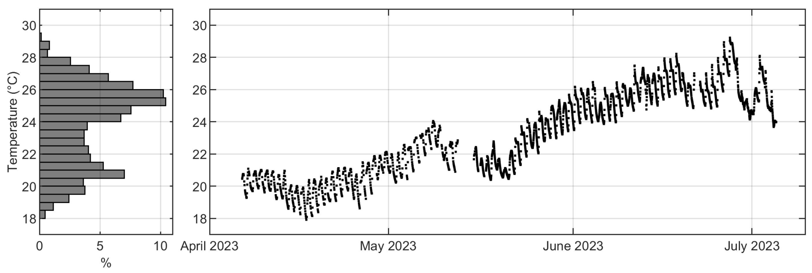
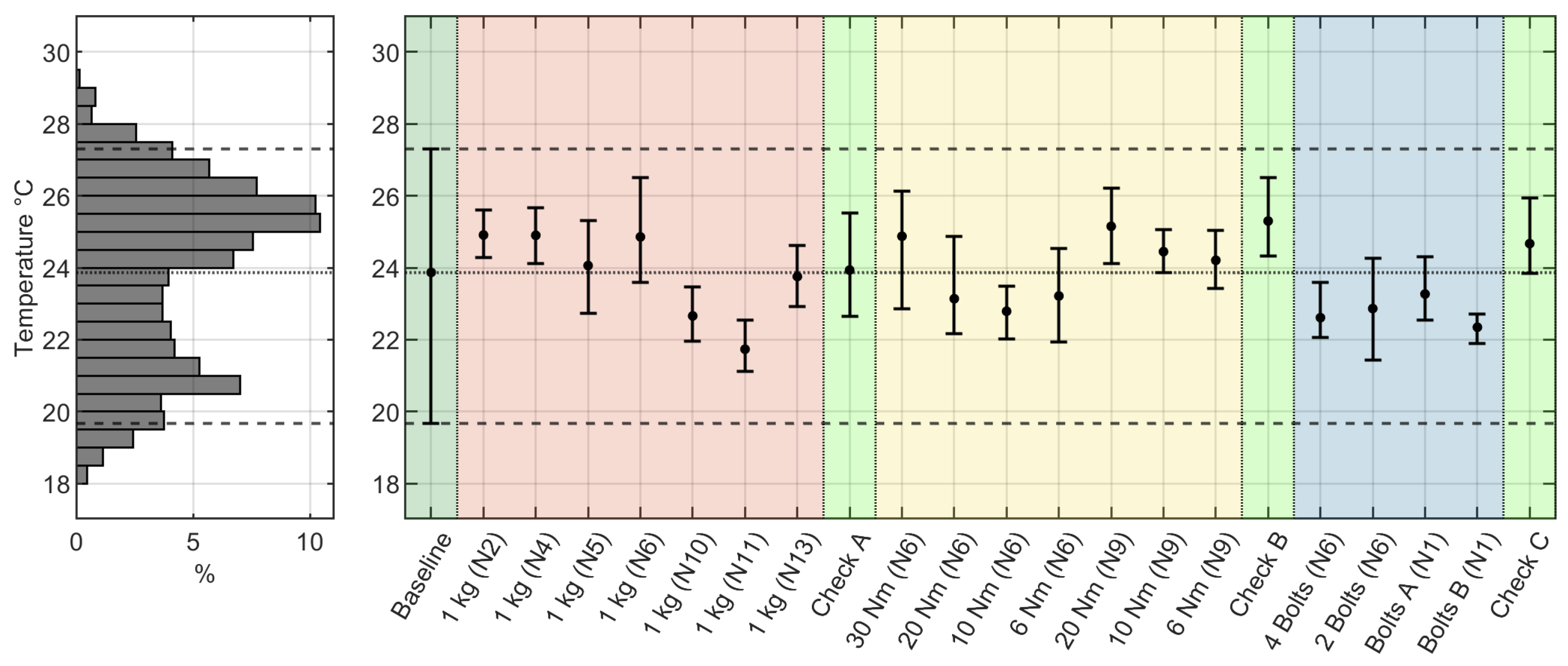
This paper demonstrates how this approach can be exploited to enhance long-term vibration monitoring through validation on a laboratory truss structure subject to environmental thermal variability and artificial damages. Anyway, these kinds of models are intended to be used for typical vibration-based SHM applications such as buildings [42], bridges [28], aerospace applications [5] and others. Moreover, the CNN-VAE model has the potential to be easily integrated with other SHM approaches, such as OMA, when used as a generative model for frequency domain data synthesis.

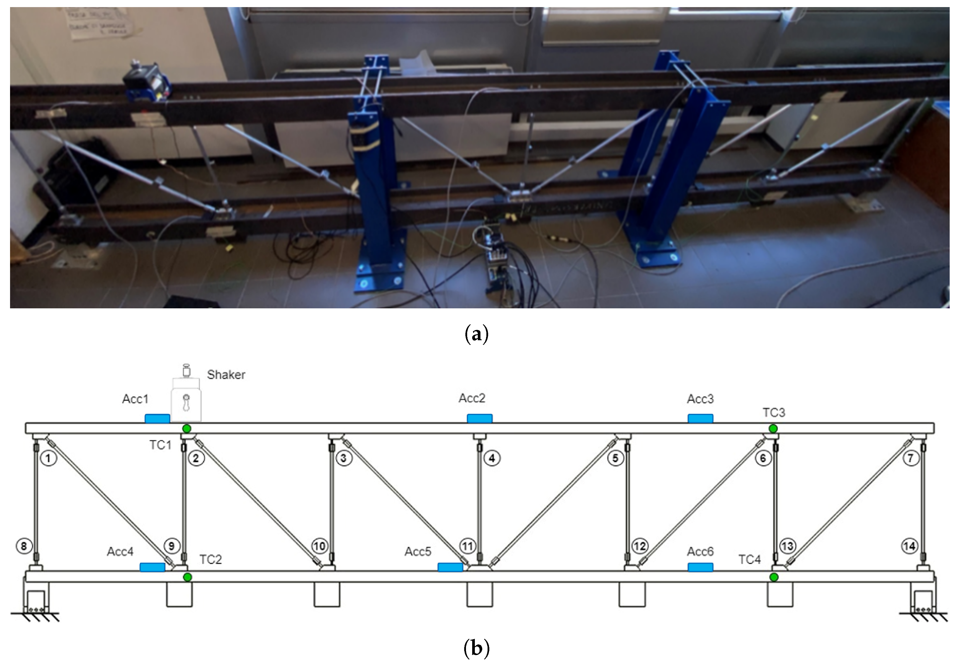
The paper is structured as follows. Section 2 describes the experimental setup of the laboratory structure and the measurement campaign with both healthy and artificially damaged structures. This section also briefly recalls the basic concepts of OMA. Section 3 introduces the proposed methodology step-by-step, from vibration frequency domain data organisation as model input to the CNN-VAE architecture and the training approach. This section also describes how to deal with the latent variables and the methods adopted to generate synthetic data. 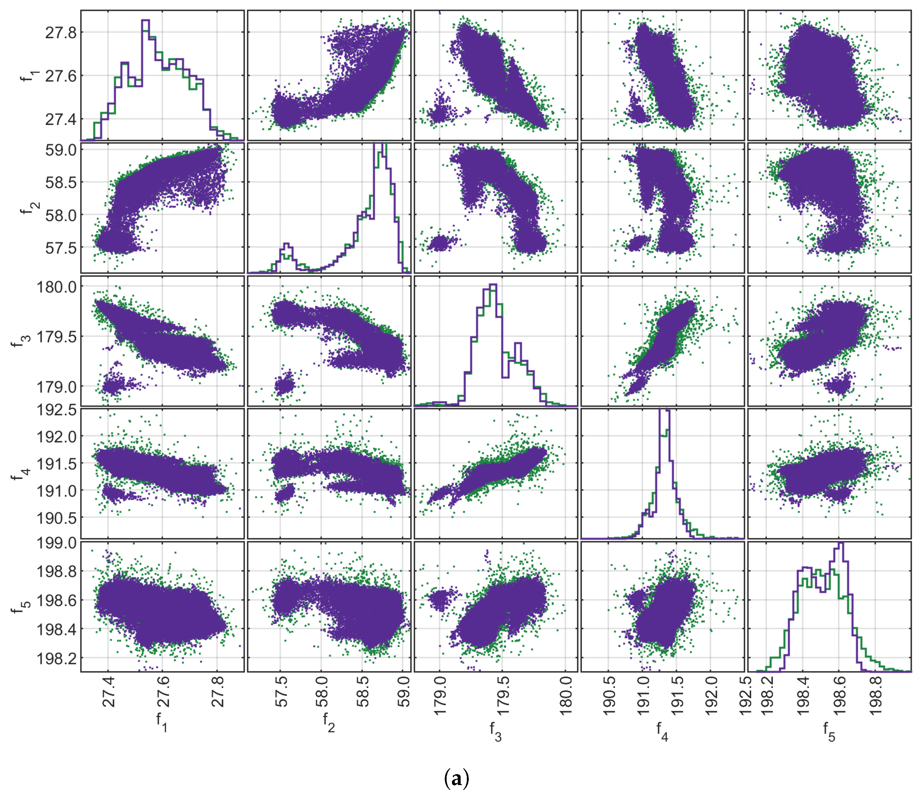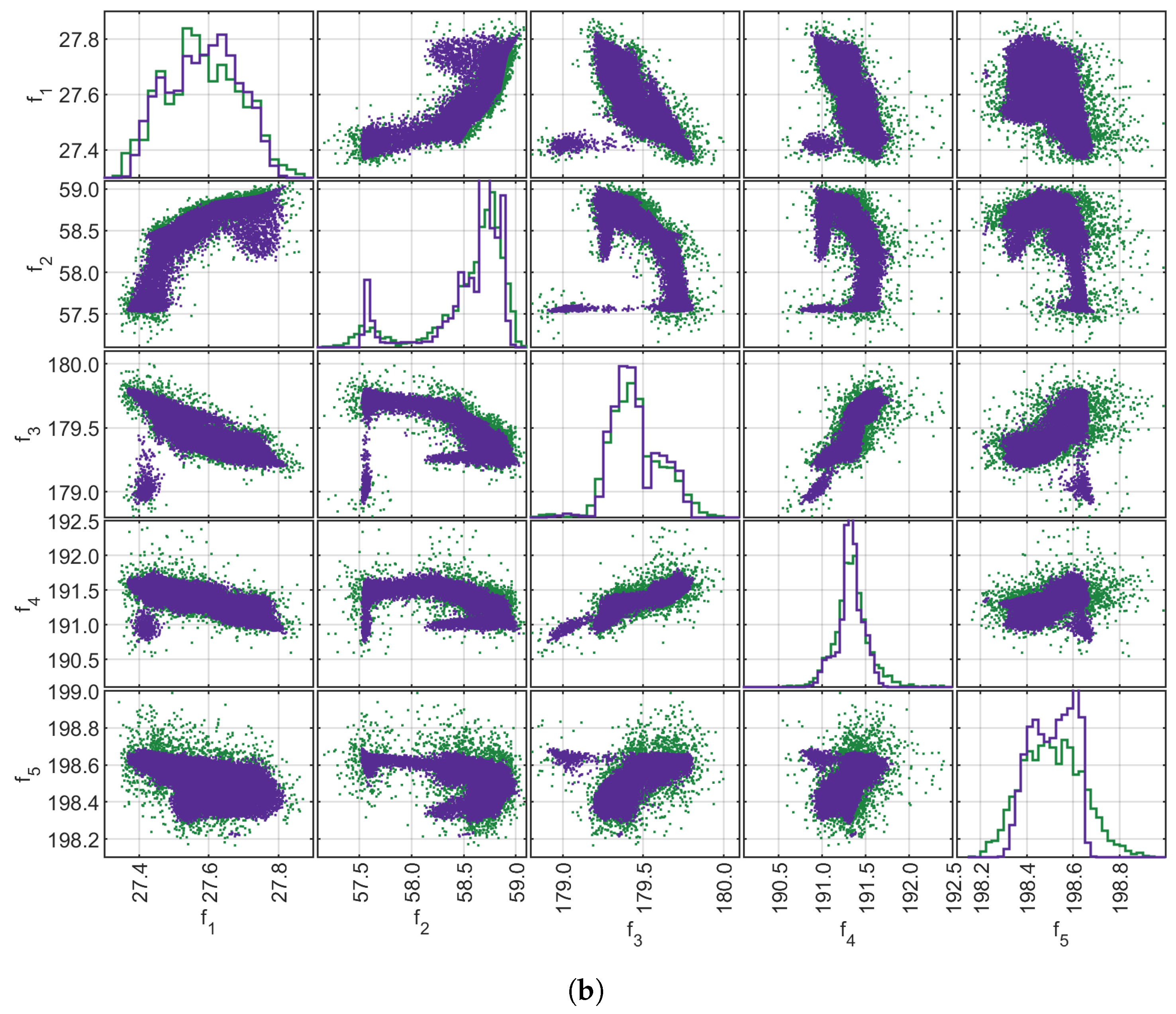Section 4 shows the training of the CNN-VAE model specifically for the experimental benchmark structure and provides an evaluation of the performance achieved. 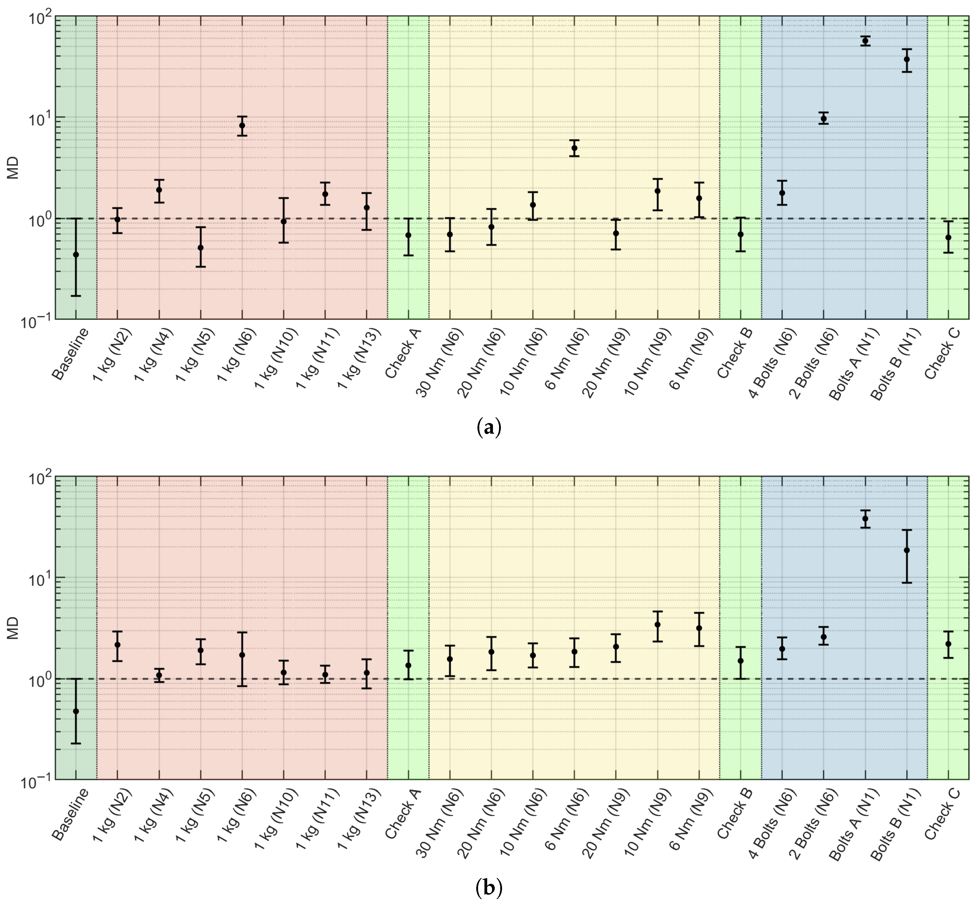Section 5 shows the results obtained using the same CNN-VAE model for two different SHM approaches. The first is used as a generative model for baseline balancing with respect to EOV combined with OMA. The second is the use as feature extractor applied to SHM, where latent variables are used to define a novelty index. Finally, Section 6 discusses the results obtained and Section 7 draws the main conclusions on the methodology presented.

2. Experimental Setup and Operational Modal Analysis

2.1. Benchmark Structure and Measurement Setup

The benchmark of the study is a simple truss structure installed in the laboratory at the University of Parma for SHM purposes (Figure 1) [43]. The structure is a classical two-dimensional Pratt truss girder with an overall span of 4.20 m and a height of approximately 0.80 m. Both bottom ends of the structure are linked to the ground supports with roller-type connections made by Teflon elements, tightened with a clamp system to allow for thermal dilatations. The diagonal and vertical members are aluminium rods with a hexagonal cross-section (12 mm across flats) and lengths of 500 or 700 mm, while the horizontal members consist of two steel H-beams, 4.30 m long and 1.1 cm thick. To improve structural stability and adjust the natural frequencies, seven rectangular masses of 15 kg each are placed at the bottom nodes of the truss. The total mass of the structure is about 300 kg. The entire structure is kept vertical by four struts located at one-third and two-thirds of the total span. The interaction between the struts and the upper beam is achieved through four stainless steel cylindrical elements which act as rollers, allowing for only vertical movement.

The truss structure is located in a laboratory environment where natural ambient excitation is not enough for vibration measurements and reliable modal parameter extraction with OMA. For this reason, an electrodynamic PCB Piezotronic model 2007E shaker (Depew, NY, USA) is mounted on the truss to excite the system in the vertical direction using a band-limited controlled white noise input signal [43]. The input control strategy ensures that the actual random excitation force has as flat a spectrum as possible. In fact, output-only OMA assumes a broadband excitation of the structure, ensuring that all structural modes in that frequency range are excited and can be detected [44]. Vibration output of the structure is monitored using six low-cost triaxial MEMS accelerometers (model TE4030) with a sensitivity of 1000 mV/g and a measurement range of ±2 g. Each sensor has a mass of about 50 g, which is negligible with respect to the total mass of the structure. The number of sensors has been deliberately kept low to replicate a realistic monitoring scenario. Environmental temperature is measured with four type K thermocouples placed in different positions, covering the whole geometry of the structure in order to highlight possible thermal gradients. All signals are generated and acquired through a National Instruments data acquisition system. The sampling rate is 2048 Hz. The modules’ built-in anti-aliasing filters prevent aliasing. To monitor and characterise the dynamic behaviour of the structure and the environmental conditions, a custom software based on LabVIEW 2020 manages the data acquisition system. The software automatically executes excitation and transducer measurements every 30 min. Each acquisition lasts 10 min. Raw time data from each test are stored in binary files, which are imported into MATLAB 2024b for the processing phase. The thermocouple signals are temporally and spatially averaged to monitor the environment temperature, thus giving a single general value for each test. For the structure response, Welch’s method is chosen to estimate auto-powers and cross-powers that form the CSM of the acceleration signals using the Hanning window, 50% of overlap and a block size of 10 s, thus having a spectral resolution of 0.1 Hz. For all the studies presented in this paper, the frequency range of analysis is 14–270 Hz where the modes of interests are located [18], corresponding to $F=2560$ spectral lines, while only the accelerations in the vertical direction are considered, thus having $N_{\mathrm{sig}}=6$ signals. Therefore, the structure response CSM is $\mathbf{G}\in {\mathbb{C}}^{N_{\mathrm{sig}}\times N_{\mathrm{sig}}\times F}$, which denotes the whole 3D CSM. The 2D complex covariance matrix of size $N_{\mathrm{sig}}\times N_{\mathrm{sig}}$ for each frequency in the discrete spectrum $f_k$ is indicated by $\mathbf{G}\left(f_k\right)$.

2.2. Modal Parameters Extraction

A typical approach for SHM is to perform OMA, using only the vibration output of the structure [44,45], and monitor the modal parameters over time. In this work, the modal parameters extraction is based on a Frequency Domain Decomposition (FDD) algorithm [46,47,48]. For each temporal frequency f or angular frequency $\omega =2\pi f$, this technique uses the structure output CSM $\mathbf{G}\left(\omega \right)$ and its Singular Value Decomposition (SVD):

$$\mathbf{G}\left(\omega \right)=\mathbf{U}\left(\omega \right)\mathbf{S}\left(\omega \right){\mathbf{U}}^H\left(\omega \right)$$

(1)

where

• $\mathbf{S}\left(\omega \right)$ is the matrix of singular values, i.e., a diagonal matrix with real and positive entries sorted in descending order $s_1\left(\omega \right)\ge s_2\left(\omega \right)\ge \dots \ge s_N\left(\omega \right)$;
• $\mathbf{U}\left(\omega \right)$ is the matrix of singular vectors $[{\mathbf{u}}_1\left(\omega \right),{\mathbf{u}}_2\left(\omega \right),\dots ,{\mathbf{u}}_N\left(\omega \right)]$ that form a unitary matrix (i.e., $\mathbf{U}{\mathbf{U}}^H=\mathbf{I}$).

In this case the SVD has this form due to the hermicity of the CSM, i.e., $\mathbf{G}\left(\omega \right)={\mathbf{G}}^H\left(\omega \right)$ Both singular values and singular vectors are a function of the frequency. The first singular value $s_1\left(\omega \right)$ reaches a local maximum and becomes dominant close to the natural frequency ${\omega }_m$ of a structural mode. In such cases, the CSM $\mathbf{G}\left(\omega \right)$ is approximately a rank one matrix, and the first singular vector ${\mathbf{u}}_1\left({\omega }_m\right)$ is a good estimate of the mode shape with unitary normalisation. Therefore, $s_1\left(\omega \right)$ can be used as a Mode Indicator Function (MIF) to detect the modes and track the natural frequencies.

In practice, the spectral data are only known at discrete frequencies depending on the frequency resolution. The most straightforward approach to identify a structural mode is the Peak Picking approach, where the frequencies of the maxima of $s_1$ and the corresponding ${\mathbf{u}}_1$ are taken respectively as modal frequency and mode shapes. However, the finite spectral resolution is an issue for SHM purposes, where a fine tracking of ${\omega }_m$ is necessary. Therefore, in this work, natural frequency estimation is performed using the approach suggested in [49]. This is based on the approximation of the peak in the discrete singular value spectrum with the behaviour of a single degree of freedom (SDOF) system:

$$\underset{\omega \to {\omega }_m}{s_1\left(\omega \right)}\approx \Re \left({\displaystyle \frac{2c_m}{\mathrm{i}\omega -{\lambda }_m}}\right)=\Re \left({\displaystyle \frac{2c_m}{{\eta }_m+\mathrm{i}(\omega -{\omega }_{dm})}}\right)$$

(2)

where ${\lambda }_m={\eta }_m+\mathrm{i}{\omega }_{dm}$ is the pole of the SDOF system, ${\omega }_{dm}$ is the damped frequency, ${\eta }_m$ is the real part of the pole and $c_m$ is a real coefficient. It follows that the natural frequency can be computed as ${\omega }_m=\sqrt{{\eta }_m^2+{\omega }_{dm}^2}$. The function in Equation (2) is fitted to the discrete singular value spectrum around a modal peak to estimate the modal frequency ${\omega }_m$ by means of Least Squares Fitting. For conciseness, this approach is referred to in this paper as Peak Fitting (PF). It has been proven that this approach overcomes the limitations imposed by the spectral resolution [49]. The FDD has been adopted in this paper, together with PF, due to its effectiveness and simple implementation. It is worth clarifying that other frequency domain modal analysis techniques can be used in combination with the CNN-VAE model presented in this paper. The main requirement is that the technique uses a CSM as input, or similar complex matrices such as the matrix of Frequency Response Functions used in Experimental Modal Analysis [50].

2.3. Measurement Campaign

The first part of the measurement campaign was dedicated to the structure in a healthy condition and involved about three months of monitoring, from April to early July 2023, for approximately 3000 measurements taken during this period that serve as the baseline data. The main EO factor acting on the structure is the ambient temperature ranging from 18 to 30 °C, as shown in Figure 2. All CSMs from vibration response measurements are normalised to have the same overall level, as explained later on in the paper (Section 3.2, Equation (3)). The baseline measurements have been processed, as described in the previous sections, to estimate the natural frequencies by means of PF and the mode shapes to set up a standard SHM approach. The sample distribution for the spectrum of the maximum singular value $s_1\left(f_k\right)$ is depicted in Figure 3. This is used as an MIF to estimate the natural frequencies $f_m$ using the PF technique described in Section 2.2. For SHM purposes, $M=5$ modes are selected. Figure 4 shows the distribution of natural frequencies for the structure in a healthy condition. According to the MIF and natural frequency distributions, the monitoring bands $B_m$ reported in

Table 1. Bands of analysis $B_m$ to monitor natural frequencies of structural modes. Lower and upper frequencies of the intervals are expressed in hertz.

	${\mathit{B}}_1$	${\mathit{B}}_2$	${\mathit{B}}_3$	${\mathit{B}}_4$	${\mathit{B}}_5$
Lower	25	55	177	189	196
Upper	30	60	183	194	202

have been identified. The most meaningful changes due to structural conditions and EOV are expected in these spectral bands.

The second part of the measurement campaign is performed in a damaged condition to test the SHM method. These measurements are carried out by creating three different types of artificial damage in different nodes:

• Added mass: 1 kg mass is placed on the structure.
• Bolt Torque: the torques of all bolts at a given node are changed with respect to the nominal torque of 12 Nm.
• Bolt Removal: only a fraction of the bolts are left at a given node with respect to the complete junction with six bolts.

A complete overview of the combination of damage type and location on the structure is provided in

Table 2. Artificial damage tests. The available combinations of damage type and location are marked with “√”.

Damage Type		Damage Location
		N1	N4	N5	N6	N9	N10	N11	N13
Mass	1 kg		√	√	√		√	√	√
Bolt Torque	30 Nm				√
	20 Nm				√	√
	10 Nm				√	√
	6 Nm				√	√
Bolt Left	2 Bolts	√			√
	4 Bolts				√

. After the tests of each artificial damage type, the structure is restored to the healthy state to check its behaviour. These tests are named “Check A/B/C” in the rest of the paper. Figure 5 shows the temperature ranges for each experimental measurement condition, proving that the range observed during the baseline period covers all artificial damage and check conditions. Hence, no unobserved temperatures occurred during the various damage tests.

3. Methodology

The approach presented in this paper proposes modelling the frequency domain structural response, in terms of CSM, using a CNN-VAE architecture with a twofold objective:

• To obtain a generative model capable of producing synthetic data consistent with the experimental observations;
• To extract representative features from the measured spectral data.

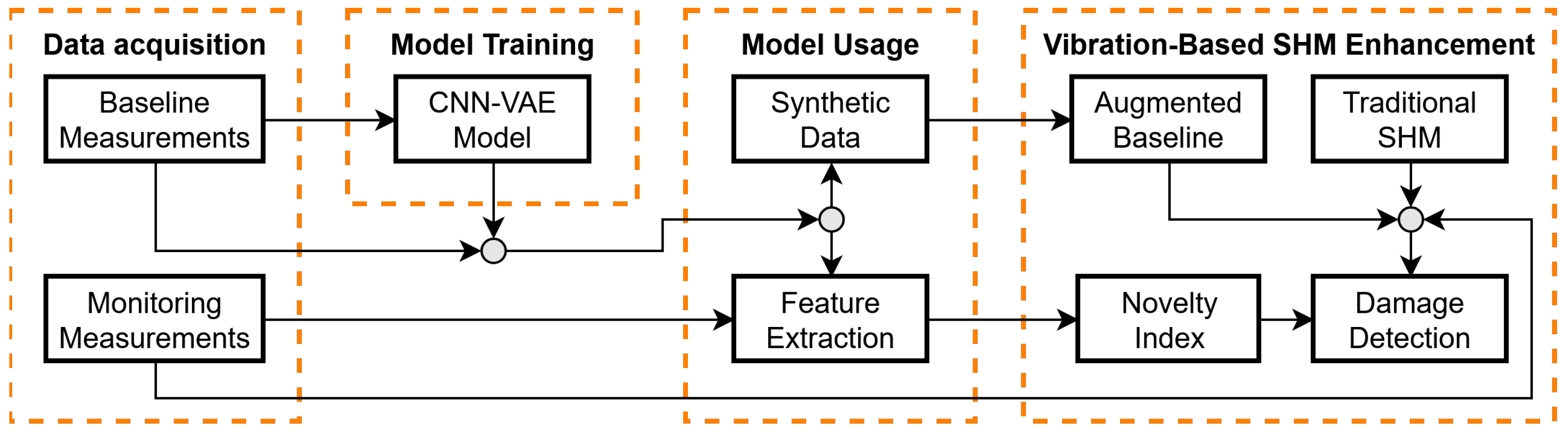
In fact, CNNs’ capabilities are used to learn spectral features of healthy structure from baseline data, while VAEs are powerful generative models that produce realistic synthetic samples “similar” to training data. Essentially, the features extracted are sensitive to the most influencing factors in the reference conditions, accounting for structural dynamics and EOV, and can be used as “monitoring features”. In addition, these control the generation of synthetic structure responses that mimic the variability of real measurements for the healthy structure. The flowchart depicted in Figure 6 shows how to integrate a CNN-VAE model with vibration-based SHM. The model can be used to implement an SHM approach directly relying on the features learned from the baseline dataset. Otherwise, traditional SHM techniques based on frequency domain data can take advantage of possible baseline augmentation strategies, exploiting the CNN-VAE as a generative model.

This section of the paper is dedicated to the general description of the building blocks of the proposed approach. A short introduction of VAEs and their classic implementation is presented, since it is the same as the implementation adopted here. Then, the approach used to encode the CSM into a format more suitable for modelling and generation is then presented. The last sections deal with the custom Enhanced LF introduced for training, the structure chosen for the CNN-VAE model and, finally, the approach to encode input data in features and how to use them for synthetic data generation. Although the following sections present and discuss one aspect at a time, the choice of some parameters and ideas intersect with each other. In the remaining part of the paper, this methodology is applied to the case study presented in Section 2.1, but the approach developed and presented here can also be applied to analogous cases for modelling structure frequency domain output in terms of CSMs.

3.1. Variational Autoencoders (VAEs)

In the branch of deep learning, AEs [51] are a type of neural network that is capable of two core tasks: encode high-dimensional input data into a low-dimensional latent representation and decode it to produce a reconstruction of the input data. Therefore, an AE is a dual network made up of an Encoder, whose task is to learn an efficient representation of the input data, and a Decoder that is responsible for generating copies faithful to the original data using the latent representation. The deterministic latent representation of input data learnt by AEs can be used both for dimensionality reduction or feature extraction. Moreover, these models are widely used in SHM applications for anomaly/novelty detection by monitoring the latent space or the reconstruction error of new observed data [26,36,39,52].

A generalisation of the standard AE is the VAE [24,53]. This paradigm of deep neural network retain the same general architecture of standard AEs, but introduces a key difference: a probabilistic framework. In fact, VAEs treat the latent variables as random variables that are represented by probability distributions, rather than deterministic values. The probabilistic formulation yields two main advantages. On the one hand, the latent space is continuous and more suitable for meaningful interpolation. On the other hand, new samples similar to the input data can be generated by means of random sampling from the latent distribution. This makes the generation capabilities of VAEs far superior to those of standard AEs, making them one of the main types of generative models. Other models, such as SAEs [54], can learn efficient and more interpretable representation in latent space but they suffer the same AE issues as generative models. Conversely, Generative Adversarial Networks (GANs) [55] are powerful generative models, but they do not naturally extract features from input data. Hence, the final choice of model type falls on VAEs, essentially because they effectively combine dual capabilities in a unique model. In fact, VAEs learn a latent representation of input data and concurrently act as a generative model.

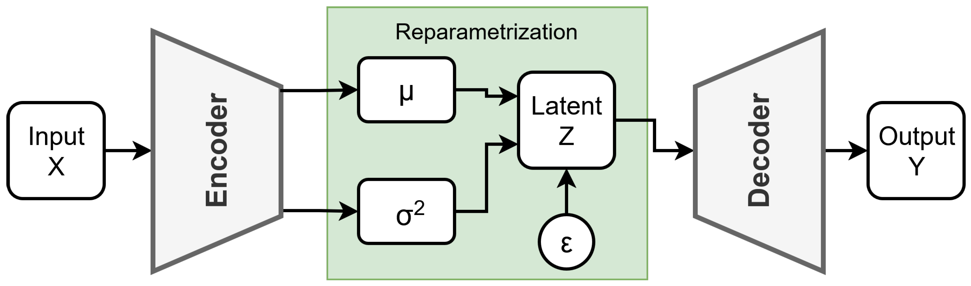
The typical implementation of VAEs is depicted in Figure 7, and it is the same as the implementation adopted in this work. The Encoder is a function that maps the input data X into a set of random latent variables Z, each with its own probability distribution. In this case, each latent variable is represented by a Gaussian $Z\sim \mathcal{N}(\mu ,{\sigma }^2)$. According to the reparametrisation trick [24], the randomness of each latent variable is provided by an external random generator that samples values $\epsilon$ from a standard Gaussian, i.e., $\epsilon \sim \mathcal{N}(0,1)$, while the actual Encoder outputs correspond to the parameters of each latent distribution, i.e., means $\mu$ and variances ${\sigma }^2$. In this way, each input X is deterministically encoded into a vector of means $\mu$ and variances ${\sigma }^2$ for all the latent variables representing each particular input into a multivariate Gaussian in the latent space. Random samples for each latent variable are drawn by means of proper scaling and offset according to the probability distribution parameters provided by the Encoder, i.e., $Z=\mu +\epsilon ·\sigma$. Thereafter, the values of latent variables Z are passed through the Decoder network, which produces the final VAE output Y, which is an approximation of the input X. Therefore, the reparametrisation trick decouples the randomness from the trainable Encoder/Decoder network parameters, thus allowing for the calculation of gradients for network training, making the encoding of X into probability distribution parameters a deterministic process.

3.2. From Spectral Data to VAE Input

The vibration output of the structure is available in the frequency domain using pre-processing, mentioned in Section 2.1, to estimate the 3D CSM $\mathbf{G}$ of measured signals for a discrete set of frequencies. In order to achieve effective data modelling with VAEs, the input data is organised relying on the following considerations:

1.

A proper CSM is a complex covariance matrix with some fundamental mathematical properties [41]. In fact, any CSM is a Hermitian matrix, must have a real positive diagonal and must be a definite positive matrix. Therefore, any model must generate synthetic data that fulfils the properties of a valid CSM. Moreover, the hermicity of $\mathbf{G}\left(f\right)$ implies that part of the matrix is redundant and provides no additional information.

2.

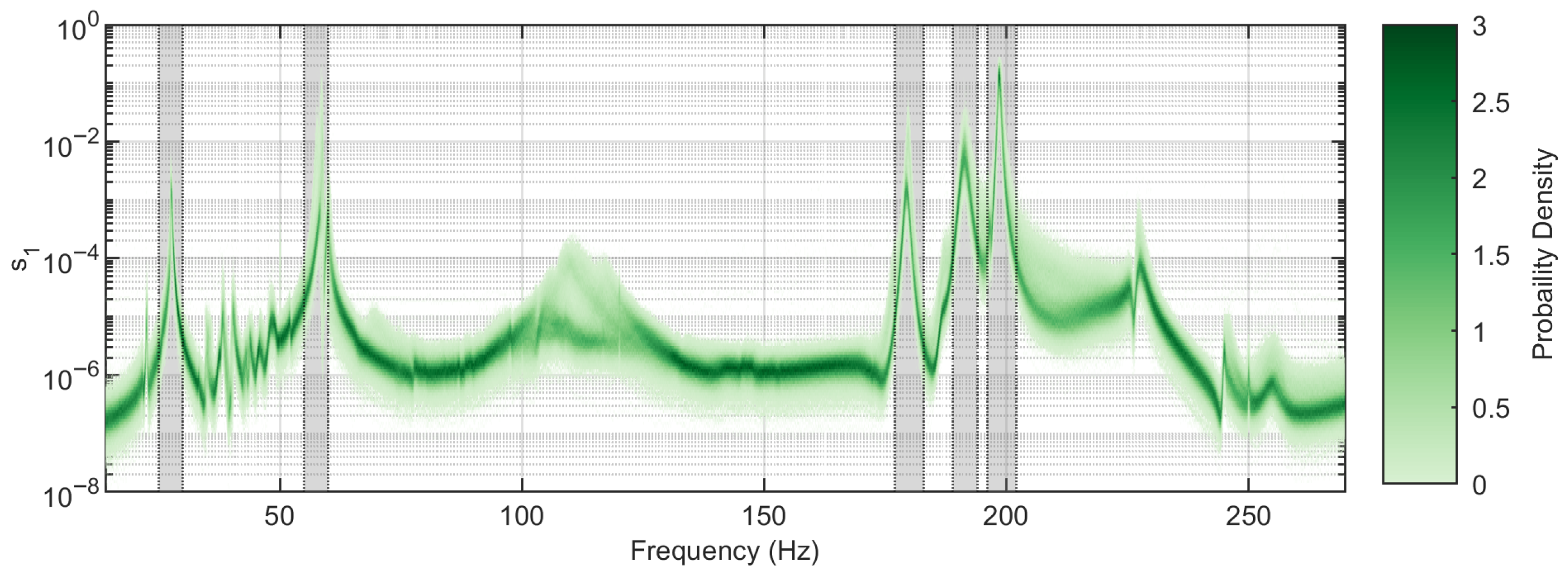
The structure response is dominated by the resonances in some bands, while the others have a much lower level, even three to five orders of magnitude below the resonance peaks (Figure 3). The main risk is that the lower zones of the spectra are treated as noise and not as a meaningful part of the data. Anyway, this may strongly penalise both the data reconstruction accuracy and the sensitivity of latent features to those bands if not handled properly.

3.

The structure response magnitude depends on the level of excitation, thus meaning that the actual level can vary between different measurements.

In order to address both these theoretical and practical aspects, the raw CSMs $\mathbf{G}$ estimated from measurements are pre-processed by means of a set of preliminary transformations for more robust and effective modelling with VAE.

The first operation, which addresses the last of the aspects mentioned in the list above, is the normalisation of the measured CSMs considering the whole spectrum. This operation is performed by multiplying each CSM by a factor in order to have the same overall Root-Mean-Square (RMS) for all measurements. The RMS value is computed using the amplitude of all the elements in the 3D CSM $G_{i,j}\left(f_k\right)$ as follows:

$$RMS\left(\mathbf{G}\right)=\sqrt{{\displaystyle \frac{1}{N^{2}F}}\sum _{\forall i,j,k}{\left|G_{i,j}\left(f_k\right)\right|}^2}$$

(3)

The uniformity of the overall level among all VAE input data makes the model “equally” sensitive to all measurements in the baseline and keeps as the most meaningful aspect the “shape” of the structure response over frequency and over sensors.

The next step is a cornerstone of the proposed approach since it enables an advantageous organisation of the CSM $\mathbf{G}\left(f\right)$ as VAE input and the control of the CSM properties generated by the model. Therefore, the first issue mentioned at the beginning of this section is resolved using the Cholesky decomposition of $\mathbf{G}\left(f_k\right)$, which is a form of matrix factorisation that represents the covariance matrices as follows:

$$\mathbf{G}\left(f_k\right)=\mathbf{L}\left(f_k\right)\mathbf{L}{\left(f_k\right)}^H.$$

(4)

Therefore, the CSMs can be represented for each frequency as the product of a lower complex triangular matrix $\mathbf{L}\left(f_k\right)$, named the Cholesky factor, and its conjugate transpose. This is the ideal candidate for preparing the CSM as VAE input for multiple reasons:

• The decomposition is unique and holds the same information of the original CSM;
• The Cholesky factor is a lower triangular matrix with no redundancy in its entries;
• The diagonal elements of the Cholesky factor are real and positive ($L_{ii}>0$), if the original CSM is a positive definite matrix;

The first two properties are ideal to guarantee that the information remains the same but it is condensed in the lower triangular part of the matrix, since the triangular part above the diagonal is null. The third property makes it straightforward to impose the condition of having a positive definite CSM $\mathbf{G}\left(f_k\right)$, since it is sufficient to constrain all diagonal elements of the Cholesky factor to be real and positive ($L_{ii}\left(f_k\right)>0$). The application of this constraint will be discussed later on in this section in the definition of the Decoder network. Finally, the diagonal elements of the Cholesky factors are the conditioned standard deviations on all preceding variables. These represent the remaining standard deviation in a variable after the linear dependence on previous variables has been removed, by starting from $L_{11}\left(f_k\right)=\sqrt{G_{11}\left(f_k\right)}$ [41,56]. Therefore, as a further benefit of the Cholesky factorisation, the terms in $\mathbf{L}\left(f_k\right)$ are proportional to standard deviations, i.e., proportional to the square root of variances in $\mathbf{G}\left(f_k\right)$; hence, their dynamics is reduced analogously to the off-diagonal terms.

The next step is the reshaping of the 3D complex matrix into a 2D real matrix. Firstly, the lower triangular part of the Cholesky factor $\mathbf{L}$ is vectorised and the null entries of the upper part are ignored. Then, since there are still complex numbers because of off-diagonal terms, the vector is made real by splitting into adjacent elements the real and imaginary parts:

$${\mathbf{L}}_{\Re v}\left(f_k\right)=\left[\begin{array}{ccccccccc}{L}_{11}& \Re \left(L_{21}\right)& \Im \left(L_{21}\right)& \dots & L_{22}& \Re \left(L_{21}\right)& \Im \left(L_{21}\right)& \dots & L_{N_{\mathrm{sig}}{N}_{\mathrm{sig}}}\end{array}\right]\left(f_k\right).$$

(5)

Therefore, a single frequency of spectral data $\mathbf{G}\left(f_k\right)$ has been encoded in a real row vector ${\mathbf{L}}_{\Re v}\left(f_k\right)$ of length $C=N^2$. The matrix serving as the VAE input is obtained by stacking all of these vectors, forming a real two-dimensional matrix $\mathbf{X}\in {\mathbb{R}}^{F\times C}$ as follows:

$$\mathbf{X}=\left[\begin{array}{c}{\mathbf{L}}_{\Re v}\left(f_1\right)\\ {\mathbf{L}}_{\Re v}\left(f_2\right)\\ ⋮\\ {\mathbf{L}}_{\Re v}\left(f_k\right)\\ ⋮\\ {\mathbf{L}}_{\Re v}\left(f_F\right)\end{array}\right].$$

(6)

Each row of the data “image” $\mathbf{X}$ contains the response of the structure at a single discrete frequency $f_k$ and contains the relationship between the response of the structure measured by the different sensors represented in terms of elements of the Cholesky factor. Clearly, the order of the sensors, and consequently the order of the Cholesky elements, must be consistent throughout the measurements and the analyses.

After the organisation of the VAE input according to Equation (6), a final operation can be necessary depending on the characteristics of the experimental data (structure modes, sensor locations, etc.). In fact, as mentioned at the beginning of this section, the amplitude of the structure response spectrum is dominated by its resonances in some bands, while other regions of the spectrum exhibit a much lower level. This can lead to a model that learns faithfully only the peaks of the frequency response, while ignoring the other bands. This issue is partially mitigated by the Cholesky factorisation, but it may not be sufficient for an effective modelling. Therefore, a non-linear scaling function of the data, serving as compression of data dynamics, is proposed. The following function can be applied to each element of VAE input $\mathbf{X}$, denoted by $X_{kc}$, to scale original data:

$$x_{\mathrm{scaled}}=sign\left(x_{\mathrm{orig}}\right){\left|x_{\mathrm{orig}}\right|}^{1/r}$$

(7)

where $sign(·)$ denotes a function that returns 1 for positive values and $-1$ for negative values. This expression keeps the sign of the original value $x_{\mathrm{orig}}$ but uses the fractional exponent to rescale its amplitude depending on the parameter r. Conversely to a simple $r^{\mathrm{th}}$ root, this can be fine-tuned and adapted to any dataset by varying the parameter r, in conjunction with the choice of the normalisation applied. Clearly, for integer odd values of r, it boils down to a regular $r^{\mathrm{th}}$ root. Unlike a non-linear scaling based on logarithms, this circumvents the singularity for null values. The scaled values $x_{\mathrm{scaled}}$ can be brought back to the original scale by applying the inverse function

$$x_{\mathrm{orig}}=sign\left(x_{\mathrm{scaled}}\right){\left|x_{\mathrm{scaled}}\right|}^r.$$

(8)

All the operations described in this section are used to prepare raw spectral data for the training of the VAE, i.e., the baseline, but also for new monitoring data provided to the model.

3.3. Training of VAE

The training of the VAEs is performed by maximising an objective function, i.e., the Evidence Lower Bound (ELBO) [53]. The optimisation is achieved by minimising an LF, defined as the negative of ELBO, that combines two terms:

• Reconstruction Loss ${\mathcal{L}}_{rec}$ encourages the Decoder to accurately reconstruct the input from latent representation. This is typically implemented as the Sum of Squared Error (SSE) between the Encoder input $\mathbf{X}$ and the Decoder output $\mathbf{Y}$, often referred to as “$L2$-Loss”.
• KL Loss ${\mathcal{L}}_{KL}$ encourages the Encoder to map all the inputs into a distribution similar to a chosen prior distribution, favouring a compact and continuous latent space, and acting as regulariser for the model. This term is the Kullback–Leibler divergence between the actual latent distribution and the standard Gaussian $\mathcal{N}(\mathbf{0},\mathbf{I})$, chosen here as prior.

The Reconstruction Loss ${\mathcal{L}}_{rec}$ is computed as

$${\mathcal{L}}_{\mathrm{rec}}={\displaystyle \sum _k^F}{\displaystyle \sum _c^C}{(Y_{kc}-X_{kc})}^2={\parallel \mathbf{X}-\mathbf{Y}\parallel }_F^2$$

(9)

where the element-wise squared error between the Decoder output $Y_{kc}$ and Encoder input $X_{kc}$ is computed and then summed, thus resulting as equal to the Frobenius norm of the difference between output and input matrices. The second term of LF can be analytically expressed in terms of $\mu$ and ${\sigma }^2$ for each latent variable, given the choice of standard Gaussian $\mathcal{N}(\mathbf{0},\mathbf{I})$ as prior distribution; hence, the KL Loss ${\mathcal{L}}_{KL}$ is

$${\mathcal{L}}_{KL}=-{\displaystyle \frac{1}{2}}{\displaystyle \sum _i^{N_{\mathrm{lat}}}}\left(1+log\left({\sigma }_i^2\right)-{\mu }_i^2-{\sigma }_i^2\right).$$

(10)

The typical LF for training a VAE can be expressed as

$${\mathcal{L}}_{\mathrm{VAE}}={\mathcal{L}}_{\mathrm{rec}}+\beta {\mathcal{L}}_{\mathrm{KL}}$$

(11)

where $\beta \ge 0$ is a hyper-parameter that allows us to control the balance between the accuracy of reconstruction and the regularisation of the latent space. As $\beta$ increases, regularisation of the latent space becomes more important in training, but an excessive regularisation worsens the accuracy of reconstruction. This variant is referred to as “$\beta$-VAE” [57,58], when $\beta =1$ Equation (11) boils down to the classic VAE LF. The training is performed iterating on subsets of the entirety of the training data, typically referred to as “batches”. Therefore, each term of the LF is computed for each input in the batch and averaged over the batch size. An “epoch” is when the training over batches covers the whole set of training data. The reparametrisation trick enables the backpropagation, bypassing the stochastic part of the encoding–decoding process, and allows us to update network parameters and minimise ${\mathcal{L}}_{\mathrm{VAE}}$.

The Reconstruction Loss of Equation (9) is the basic starting point to train a model that provides a general approximation of input data. In fact, the classic $L2$-Loss endorses the reduction in “big” errors. Considering the type of data used in this paper, some portions of the spectra are prominent with respect to others and are automatically privileged in the training process. Therefore, the resonant modes are naturally favoured in this process, even though they do not have the same amplitude. Conversely, as already mentioned in the previous section, this penalises the weakest region of the spectra. Different countermeasure contributes to mitigate this aspect such as the Cholesky decomposition and the non-linear scaling of Equation (7). Despite these countermeasures, modal peaks still have different heights and can be learned by the VAE with different accuracies, since no specific information about the natural frequencies and mode shapes are introduced in the LF. However, for SHM purposes, the modes are all equally important, independently of their magnitude in the structure response spectra.

In SHM contexts, it can be advantageous to extend the LF by incorporating additional terms to improve the learned representations [6,7,34]. The aim is to make them physically consistent, interpretable or simply more accurate on some particular characteristics. This approach adds a “soft” constraint to the training process that guides the model to learn not only a mere accurate reconstruction of the data. In fact, it can be exploited to focus on specific characteristics of the data but also to respect other requirements, without imposing a rigid constraint. The approach adopted in this paper is to exploit some typical concepts from OMA and FDD to “promote learning of important characteristics” of data useful for SHM, such as natural frequency and mode shapes, without ignoring the whole structure response.

As mentioned in Section 2.2, the spectrum of the biggest singular value of $\mathbf{G}\left(f_k\right)$ is used as the MIF to detect modes and monitor the natural frequencies. For this reason, the LF is extended with two components that guarantee the fidelity of the MIF and mode shapes between experimental input data and VAE output. However, performing SVDs for each training iteration meaningfully increases the computational burden. Therefore, a fast estimation of the MIF is performed in the training phase, by exploiting two mathematical considerations. Firstly, the Frobenius norm of the Cholesky factor $\mathbf{L}$ has the following property:

$$\parallel \mathbf{L}\left(f_k\right){\parallel }_F^2=trace\left(\mathbf{S}\left(f_k\right)\right),$$

(12)

where $\mathbf{S}\left(f_k\right)$ is the singular value matrix from the SVD of $\mathbf{G}\left(f_k\right)$ (Equation (1)). Secondly, the squared Frobenius norm ${\parallel \mathbf{L}\parallel }_F^2$ is a good estimate of $s_1\left(f_k\right)$ in the proximity of the modes since the latter is dominant in those bands. According to VAE data organisation (Equations (5) and (6)), the approximate MIF can be computed in the training phase by

$$MIF(\mathbf{X},f_k)={\displaystyle \sum _{c=1}^C}{X}_{kc}^2$$

(13)

where $MIF(X,f_k)$ is a vector of length F; in fact, each element corresponds to a discrete frequency of spectral data. If no scaling is applied, Equation (13) is exactly equivalent to Equation (12); otherwise, the amplitude is squeezed by the non-linear scaling (Equation (7)). This information is useful to formulate the additional loss terms that improve the effectiveness of the VAE for SHM, allowing it to focus on the most important spectral features of structure response. This is implemented focusing on the monitoring bands $B_m$ (Table 1) and using a weighting strategy over frequency defined ad hoc to compensate different heights of the MIF for each mode peak:

$$w(X,f_k)=\left\{\begin{array}{cc}{\displaystyle 1/\underset{f_j\in B_m}{max}MIF(X,f_j)}\hfill & \mathrm{if}{f}_k\in B_m,\hfill \\ 0\hfill & \mathrm{otherwise}.\hfill \end{array}\right.$$

(14)

The weighting vector $w(X,f_k)$ basically normalises the $MIF(\mathbf{X},f_k)$ by making the maximum peaks equal to one in each band, while it cancels out the rest of the spectrum. Hence, the MIF Loss term ${\mathcal{L}}_{MIF}$ is implemented as the weighted SSE between the input and output MIFs:

$${\mathcal{L}}_{MIF}={\displaystyle \sum _k^F}{\left(w(\mathbf{X},f_k)·(MIF(\mathbf{Y},f_k)-MIF(\mathbf{X},f_k))\right)}^2.$$

(15)

Intuitively, this term makes the VAE training more sensitive to the location of the peak on the spectrum in the input data, rather than its amplitude. For this reason, ${\mathcal{L}}_{MIF}$ guides the VAE to finely follow the peak position on the spectral axis.

A similar approach is adopted to endow the training process with specific sensitivity to modal shapes. In fact, as mentioned in Section 2.2, on the resonance the structure response is dominated by the mode shape. For this reason, the Shape Loss ${\mathcal{L}}_{SHP}$ is defined as

$${\mathcal{L}}_{SHP}={\displaystyle \sum _k^F}{\displaystyle \sum _c^C}{\left(w(\mathbf{X},f_k)·(Y_{kc}-X_{kc})\right)}^2,$$

(16)

where the weighting vector $w(\mathbf{X},f_k)$ balances the response amplitude for each monitoring band, thus making each mode shape equally important in the training.

The custom Enhanced LF used to train the VAE on CSM data is

$${\mathcal{L}}_{\mathrm{VAE}}={\mathcal{L}}_{\mathrm{rec}}+{\beta }_{\mathrm{KL}}{\mathcal{L}}_{\mathrm{KL}}+{\beta }_{\mathrm{MIF}}{\mathcal{L}}_{\mathrm{MIF}}+{\beta }_{\mathrm{SHP}}{\mathcal{L}}_{\mathrm{SHP}}$$

(17)

where ${\beta }_{\mathrm{MIF}}$ and ${\beta }_{\mathrm{SHP}}$ are two additional non-negative hyperparameters that control the importance of these two additional custom terms in the LF. The terms ${\mathcal{L}}_{\mathrm{MIF}}$ and ${\mathcal{L}}_{\mathrm{SHP}}$ level out the sensitivity of the model to natural frequency shifts and variations in mode shapes, giving each mode the same “weight”. The benefits of these additional terms in the enhanced LF are shown and discussed in the rest of the paper. The CSM positivity on the Cholesky factor is not introduced in the modelling approach as a “soft” constraint since it does not prevent the occurrence of negative CSMs. Instead, a “hard” constraint is forced by means of the Decoder architecture and is discussed in the next section.

3.4. Encoder and Decoder of CNN-VAE

This section describes in detail the architecture chosen for the Encoder and Decoder based on a CNN. CNNs are a widely used class of deep learning models that allow for the hierarchical extraction of features with different levels of abstraction, while reducing the number of parameters compared to fully connected networks. The key factors that guided the choice of this architecture originate from the organisation of the structure response into a rectangular 2D real matrix, according to Equation (6), and the characteristics of spectral data. The “spatial” patterns on these pseudo-images can be effectively learnt by CNNs. In this specific case, the two dimensions represent the relationship between contiguous frequencies, along the row axis, and structural patterns, along the column axis. In fact, structural dynamic responses exhibit spectral continuity related to modal behaviour, while the structural response over sensors is encoded by the elements of Cholesky decomposition of the CSM $\mathbf{G}$. The strength of CNNs when dealing with this kind of input data is their ability to learn and generate spectral and structural patterns while maintaining a relatively small number of trainable parameters. The hierarchical feature extraction provided by successive convolutional layers makes it possible to achieve a progressive aggregation of local spectral information into higher-level representations that describe dynamic behaviour of the monitored structure. Moreover, CNNs introduce a form of invariance with respect to translations along the frequency axis. In fact, they can still recognise and generate similar patterns even if they are shifted in the spectrum. This is useful because modal peaks vary and shift due to EOV. 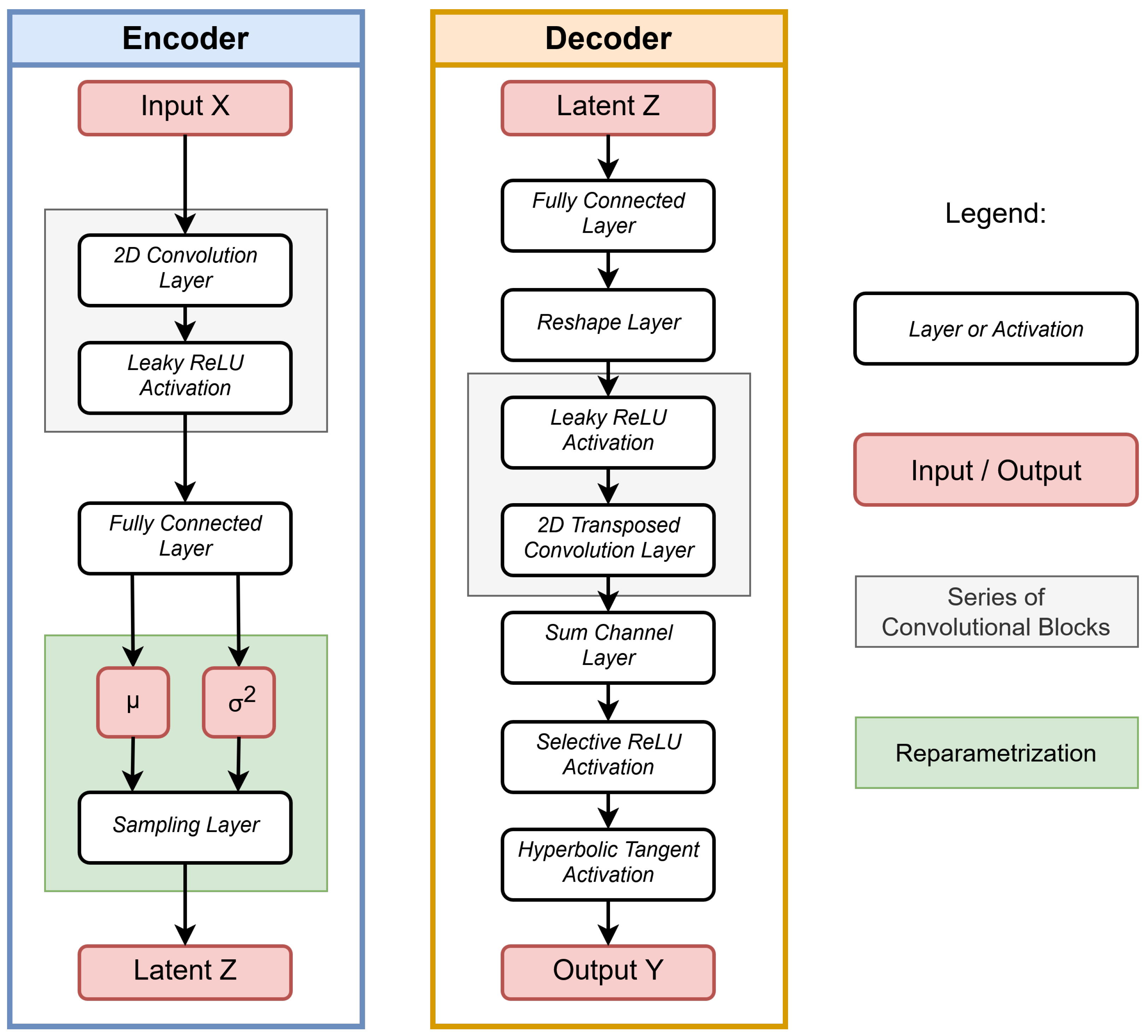The schemes of both the Encoder and the Decoder are depicted in Figure 8.

The Encoder has a 2D input with a single channel that is followed by a series of convolutional blocks. Each of these blocks is formed by a 2D convolutional layer followed by a LeakyReLU activation function. The number of consecutive blocks of this type controls the receptive field of the CNN and the depth of the network. In this application, all these blocks share the same parameters to reduce the number of hyperparameters, which are number of filters $N_{\mathrm{filt}}$, kernel size $K_F\times K_C$, stride $(S_F,S_C)$ and LeakyReLU slope for negative values a. A stride $S_F>1$ can be adopted to progressively reduce the size of the frequency axis (rows) down to the last convolutional layer. The number of reduced frequencies as output from the last convolutional block is denoted by $F_{red}$ and depends on the number of convolutional layers and the stride itself. The combination of these two parameters controls the ability of the CNN to learn features from a larger frequency range. Thereafter, the convolutional feature map of size $F_{red}\times C\times N_{\mathrm{filt}}$ is flattened by a fully connected layer that returns the parameters of the Gaussian distribution, ${\mu }_i$ and $log{\sigma }_i^2$, for each latent variable. In this implementation, the Encoder returns the logarithm of the variance $log{\sigma }_i^2$, instead of variance ${\sigma }_i^2$ itself, since it is more convenient for numerical stability. Finally, the sampling layer puts in practice the reparametrisation trick and generates Gaussian random samples $Z_i\sim \mathcal{N}({\mu }_i,{\sigma }_i^2)$ from each individual latent variable distribution.

The Decoder has a structure that mirrors that of the Encoder, but with some crucial differences. The input layer receives latent variable samples $\mathbf{Z}$, then a fully connected layer coupled with a reshape layer mixes and projects them back into a space of dimension $F_{red}\times C\times N_{\mathrm{filt}}$. At this point, the Decoder also has a series of convolutional blocks, each made up of a LeakyReLU activation function and a 2D transposed convolution layer, which progressively restores the resolution along the frequency axis, reversing the compression performed by the Encoder. In fact, these share the same parameters of convolutional blocks of the Encoder. The structural differences with the Encoder are found in the next layers. The space of size $F\times C\times N_{\mathrm{filt}}$ coming out of the previous block is squeezed back into a space of dimension $F\times C\times 1$ by a “Summing Layer” created with a simple 2D convolution, having a single $1\times 1$ kernel. This recreates a pseudo-image of the same size and shape of the input $\mathbf{X}$. At this point, one of the key elements of this model comes into play. In fact, the “hard” positivity constraint on Cholesky factors takes place by means of a custom layer, named “Selective ReLU”. This layer simply applies a ReLU function only on those columns corresponding to the diagonal elements of the Cholesky factor, according to Equation (6). This impedes negative values on the Cholesky factor diagonals for each frequency and imposes a structural constraint of non-negativity on the Decoder output. Finally, a non-linear activation function (hyperbolic tangent) produces the Decoder output $\mathbf{Y}$, keeping all values bounded in the range $[-1,1]$ for better stability.

The proposed architecture of the CNN-VAE is tailored to model this kind of spectral data. The anisotropic structure of input data and convolutions for the Encoder and Decoder give the user the possibility of tuning kernel sizes and strides independently for the frequency axis and the cross-sensor axis, according to the characteristics of specific data. For instance, the kernel size along the frequency axis can be chosen according to the frequency resolution and bandwidth of the spectral characteristics of the specific case under study. Similarly, the size of the kernel can be chosen to capture and represent the relationship between sensors. Moreover, the combination of Cholesky factorisation with Selective ReLU activation on its diagonal components removes the redundancy inherent to the hermicity of CSMs and, at the same time, imposes a structural hard constraint to generate Cholesky factors associated with (semi-)definite positive CSMs.

3.5. Latent Variables and Data Synthesis

This final section on the methodology used in this paper focuses on how to retrieve the latent representation of measured data using the Encoder and the approach adopted to generate synthetic data using the Decoder. According to the scheme in Figure 8, two kinds of outputs can be retrieved from the Encoder for a specific given input $\mathbf{X}$; one is deterministic and the other is random [59]. In the following, the subscripts $\mathcal{D}$ and $\mathcal{R}$ stand respectively for “deterministic” and “random” to specify which type of Encoder output is considered, while the Encoder function is denoted by the operator $\mathrm{ENC}(·)$. The deterministic output consists of the parameters of the latent variable distributions as

$${\mathbf{P}}_{\mathbf{X}}=\left[\begin{array}{cc}{\mathbf{P}}_{\mu ,\mathbf{X}}& {\mathbf{P}}_{{\sigma }^2,\mathbf{X}}\end{array}\right]={\mathrm{ENC}}_{\mathcal{D}}\left(\mathbf{X}\right),$$

(18)

where ${\mathbf{P}}_{\mathbf{X}}$ is the vector of distribution parameters related to a specific input $\mathbf{X}$. This vector is split in two parts, ${\mathbf{P}}_{\mu }$ and ${\mathbf{P}}_{{\sigma }^2}$, respectively, the vectors of the means ${\mu }_i$ and variances $log{\sigma }_i^2$:

$$\begin{array}{cc}\hfill {\mathbf{P}}_{\mu ,\mathbf{X}}=& {\left[\begin{array}{ccccc}{\mu }_1& \dots & {\mu }_i& \dots & {\mu }_{N_{\mathrm{lat}}}\end{array}\right]}_{\mathbf{X}}\hfill \\ \hfill {\mathbf{P}}_{{\sigma }^2,\mathbf{X}}=& {\left[\begin{array}{ccccc}log{\sigma }_1^2& \dots & log{\sigma }_i^2& \dots & log{\sigma }_{N_{\mathrm{lat}}}^2\end{array}\right]}_{\mathbf{X}}.\hfill \end{array}$$

(19)

Instead, the Encoder random output is the vector of samples $\mathbf{Z}$ for each latent variable, given the input $\mathbf{X}$. This is indicated as

$${\mathbf{Z}}_{\mathbf{X}}={\left[\begin{array}{ccccc}{Z}_1& \dots & Z_i& \dots & Z_{N_{\mathrm{lat}}}\end{array}\right]}_{\mathbf{X}}={\mathrm{ENC}}_{\mathcal{R}}\left(\mathbf{X}\right).$$

(20)

In this case, the samples are generated by feeding ${\mathbf{P}}_{\mathbf{X}}$ into the sampling layer of the Encoder that applies the reparametrisation trick. Therefore, the sample ${\mathbf{Z}}_{\mathbf{X}}$ represents a random value extracted from the latent distribution resulting from the mapping of the input $\mathbf{X}$ into the latent space.

An approach used in this paper is to mimic the usage of a deterministic standard AE, while keeping the advantages of a VAE in the latent space regularisation due to its probabilistic nature. In fact, it is useful to have deterministic mapping of a given input $\mathbf{X}$ into the latent space. This is directly achieved considering the distribution parameters returned by the Encoder ${\mathbf{P}}_{\mathbf{X}}$ (Equation (18)), instead of the random samples ${\mathbf{Z}}_{\mathbf{X}}$ (Equation (20)). Despite the differences with the deterministic latent variables of a standard AE, $\mu$ and $log{\sigma }^2$ are also parameters uniquely associated with a specific input $\mathbf{X}$ that can be used as monitoring features for SHM. This aspect will be discussed later on in the paper.

Synthetic data can be generated as the Decoder output for a generic latent vector $\mathbf{Z}$ as input. This is written as

$$\mathbf{Y}=\mathrm{DEC}\left(\mathbf{Z}\right),$$

(21)

where the operator $\mathrm{DEC}(·)$ indicates the Decoder function. Depending on the content of the vector $\mathbf{Z}$, different synthetic data can be generated. From the considerations above about the deterministic or random representation in the latent space, different approaches can be defined for synthetic data generation through the Decoder. Hence, a process named here as “Deterministic Generation” (DGEN) with the CNN-VAE is defined as

$${\mathbf{P}}_{\mathbf{X}}=\left[\begin{array}{cc}{\mathbf{P}}_{\mu ,\mathbf{X}}& {\mathbf{P}}_{{\sigma }^2,\mathbf{X}}\end{array}\right]={\mathrm{ENC}}_{\mathcal{D}}\left(\mathbf{X}\right)\to {\mathbf{Y}}_{\mathcal{D}},\mathbf{X}=\mathrm{DEC}\left({\mathbf{P}}_{\mu ,\mathbf{X}}\right).$$

(22)

Basically, this process involves mapping a specific input $\mathbf{X}$ into the latent space, bypassing the sampling layer of the Encoder and feeding the Decoder directly with the deterministic latent vector of the mean values $\mathbf{Z}={\mathbf{P}}_{\mu ,\mathbf{X}}$. In this way, the CNN-VAE generates a deterministic representation ${\mathbf{Y}}_{\mathcal{D}},\mathbf{X}$ of a desired input $\mathbf{X}$ that can be used, for instance, in model performance evaluation.

Conversely, one of the key advantages of the VAE framework is the possibility to randomly sample the latent space and produce new and unseen synthetic data. This process, named here as “Random Generation” (RGEN), with the CNN-VAE is defined as

$${\mathbf{Z}}_{\mathbf{X}}={\mathrm{ENC}}_{\mathcal{R}}\left(\mathbf{X}\right)\to {\mathbf{Y}}_{\mathcal{R}},\mathbf{X}=\mathrm{DEC}\left({\mathbf{Z}}_{\mathbf{X}}\right).$$

(23)

This approach enables the CNN-VAE to generate random variations ${\mathbf{Y}}_{\mathcal{R}},\mathbf{X}$ of a specific input $\mathbf{X}$. This approach can be used for synthetic data generation useful for SHM purposes. The Decoder output, i.e., a synthetic Cholesky factor, can be restored to the original scale by means of Equation (8) and the synthetic CSM is obtained by means of Equation (4).

4. Spectral Data Modelling with CNN-VAE

4.1. Model Definition and Training

Using the methodology introduced in the previous section, a CNN-VAE model has been developed for the specific experimental case presented in Section 2. The architecture adopted for Encoder and Decoder networks was introduced in Section 3.4 and summarised in the scheme of Figure 8. The steps involved in defining the specific model are described below. It is worth noting that the various choices were validated by verifying afterwards that they were appropriate for the purpose of the model.

The first step was the definition of the number of consecutive convolutional blocks for both the Encoder and Decoder. In this case, the number was set to three, as this depth is considered sufficient for feature extraction. In fact, increasing the number of consecutive convolutional blocks also increases the receptive field of the CNN and enables the learning of more general features from the data. Conversely, a lower number of convolutional blocks would result in a model that is more sensitive to local features in the “pseudo-images”, rather than to global ones. Thereafter, the choice of a stride $S_F=2$ along the frequency axis allows for a progressive reduction in dimensionality and enables the extraction of patterns sensitive to a wider frequency range. After three convolutional layers, the frequency axis is reduced by a factor of $2^3$, thus resulting in a reduced frequency axis of length $F_{red}=320$. Instead, the stride over column axis $S_C=1$ is adopted to keep its dimension over convolutional layers since it is already much smaller than the frequency axis. This combination of number of convolutional layers and stride is also advantageous because it reduces the number of learnable parameters with respect to an Encoder and Decoder with the same structure but with a single convolutional block. This happens since the size of fully connected layers present in both Encoder and Decoder are drastically reduced.

At this stage, a series of preliminary analyses was performed to set up the remaining hyperparameters. All the preliminary analyses were carried out using a subset of 300 measurements uniformly taken from the baseline (i.e., one tenth of the whole baseline, 50% for training and 50% for testing) and using the Classic LF (Equation (11)) without the custom terms. For the training on the small subset we used a batch size of 20, a number of epochs of 100 and a learning rate of ${10}^{-3}$. The VAE networks were trained using the ADAM optimisation algorithm [60] to minimise the LF. The first analysis was conducted to set the parameter r for non-linear scaling of input data (Equations (7) and (8)), using a first tentative CNN-VAE. The minimum value that produced satisfying results was $r=3$. Thereafter, the remaining key parameters were studied: number of convolutional filters $N_{\mathrm{filt}}$, kernel sizes $K_F$ and $K_C$, and the latent space dimension $N_{\mathrm{lat}}$. Two preliminary parametric analyses were conducted to understand the advantageous combinations that allow us to reduce the Reconstruction Loss (Equation (9)) and provide accurate reconstruction of structure response. Firstly, a rough grid of the four parameters was explored to identify the most favourable order of magnitude for each parameter. Secondly, once a plausible range was identified for each parameter, a Bayesian Optimiser was used to explore in detail the parameter subspace. The verdict of this parametric study is that a “high number of small convolutional filters” is adequate for a low Reconstruction Loss. This outcome observed on a smaller subset of data was confirmed on the whole training set used for the final model. The values of $N_{\mathrm{filt}}=48$, $K_F=3$, and $K_C=4$ were chosen. From the same analysis, it emerged that a latent dimension $N_{\mathrm{lat}}>10$ does not significantly improve the model performance in terms of Reconstruction Loss. In fact, by increasing the latent space dimension, the information is more diluted across the latent space variables, making them less informative. For this reason, $N_{\mathrm{lat}}=7$ is chosen.

The definitive model was trained using the whole baseline, which was split in two equal groups; 50% of the data was used for training and the remaining 50% was used for testing. All the parameters used to define the model and for its training are summarised in

Table A1. Constants and parameters of input data normalisation and CNN-VAE (all values are non-dimensional, unless otherwise specified).

Parameter	Symbol	Value
Input Data
Rows	F	2560
Columns	C	$N_{\mathrm{sig}}^2=36$
CSM normalisation	$RMS\left(\mathbf{G}\right)$	${10}^{-3}$${(m/s^2)}^2$
Non-linear scaling function exponent	r	3
VAE Training
Latent space dimension	$N_{\mathrm{lat}}$	7
Loss KL Divergence weight	${\beta }_{\mathrm{KL}}$	0.125
Loss MIF weight	${\beta }_{\mathrm{MIF}}$	4
Loss SHP weight	${\beta }_{\mathrm{SHP}}$	0.05
Optimiser	-	ADAM
Learning Rate (reduced every 100 Epochs)	-	${10}^{-3},{10}^{-4},{10}^{-5}$
Batch Size	-	60
Number of Epochs	-	300
Convolutional Layers
Number of filters	$N_{\mathrm{filt}}$	48
Kernel size	$K_F\times K_C$	$3\times 4$
Stride	$(S_F,S_C)$	$(2,1)$
Leaky ReLU slope for negative values	a	$0.01$

, while the layers of the Encoder and Decoder are summarised in

Table A2. CNN-VAE architecture for modelling structure response CSM in terms of Cholesky factors.

Block Type	Layers	Output Size
Encoder
Input	2D input	$F\times C\times 1$
Convolutional Blocks (3×)	2D Convolution	$F/8\times C\times N_{\mathrm{filt}}$
	LeakyReLU
Fully Connected	Fully Connected	$2N_{\mathrm{lat}}$
Output	Reparametrisation	$N_{\mathrm{lat}}$
	Sampling
Decoder
Input	Feature input	$N_{\mathrm{lat}}$
Project and Reshape	Fully Connected	$F/8\times C\times N_{\mathrm{filt}}$
	Reshape
Convolutional Blocks (3×)	2D Transp. Convolution	$F\times C\times N_{\mathrm{filt}}$
	LeakyReLU
Sum Channels	2D Convolution ($1\times 1$)	$F\times C\times 1$
Selective Activation	Selective ReLU	$F\times C\times 1$
Output	Hyperbolic Tangent	$F\times C\times 1$

. Two models were trained: one using the Classic LF of Equation (11) and one using the Enhanced LF of Equation (17). To privilege the accuracy of the reconstruction, a value of ${\beta }_{\mathrm{KL}}<1$ was chosen, while the values of ${\beta }_{\mathrm{MIF}}$ and ${\beta }_{\mathrm{SHP}}$ were tuned empirically, evaluating the performance of the trained CNN-VAE model in terms of accuracy and sensitivity to the modal behaviour of the structure. Figure 9 depicts a summary of the values for the total LF and each individual term, comparing the average on the training set with the average on the testing set. Both models show very similar results on both datasets, which may indicate that the models are not overfitting. The Reconstruction Loss ${\mathcal{L}}_{rec}$ assumes almost identical values for both models, thus meaning that the additional terms in the Enhanced LF do not degrade the model performance in terms of accuracy. The values set for ${\beta }_{\mathrm{MIF}}$ and ${\beta }_{\mathrm{SHP}}$ result in similar contributions of ${\mathcal{L}}_{\mathrm{KL}}$, ${\mathcal{L}}_{\mathrm{MIF}}$ and $\mathcal{L}{,}_{\mathrm{SHP}}$ to the Enhanced LF (between 10 and 15%).

Finally, some notes about the development platform and computational burden. The models were realised with MATLAB 2024b using a desktop computer for training equipped with an Intel Core i9 processor 14900KF, RAM 64 GB, and GPU NVIDIA T1000 8 GB. Both the Classic and Enhanced LF CNN-VAE models required about 6 h to be trained using the specified parameters and training dataset. Once trained, the model can be run on less powerful hardware, such as a laptop without a GPU (Intel Core i7-1255U and 24 GB RAM). In this case, encoding a measured CSM in latent space takes approximately 0.11 s, also including Cholesky factorisation, reshape and scaling. The complete process of data generation from a measured CSM takes approximately 0.17 s (same for DGEN or RGEN).

4.2. Model Performance Evaluation

The performance of the CNN-VAE model is evaluated here before it is used for SHM purposes. The analysis presented here focuses on capabilities as a generative model for studying the ability to replicate baseline data and the level of accuracy. With this purpose, each measurement $\mathbf{X}$ in the baseline is replicated using the CNN-VAE model by means of Equation (22) (${\mathbf{Y}}_{\mathcal{D}},\mathbf{X}$), thus obtaining the DGEN synthetic baseline. Similarly, Equation (23) is used to generate 10 samples (${\mathbf{Y}}_{\mathcal{R}},\mathbf{X}$) from each experimental measurement in the baseline and have the RGEN synthetic baseline. The quantitative comparison between synthetic and measured data is realised in the original data scale, using Equation (8) to restore the amplitude.

The basic performance analysis regards the natural frequencies $f_m$, estimated by means of PF introduced in Section 2.2, on experimental measurements and synthetic data. Figure 10 compares the result of measured data with DGEN synthetic data, also showing the difference between the CNN-VAE trained with the Classic LF and the Enhanced LF. The model trained with the Classic LF represents the most frequent behaviour but ignores rare “peripheral” behaviour. Instead, the custom terms in the Enhanced LF of Equation (17) improve the capacity of the model to better reproduce less frequent conditions. This behaviour is more evident in Figure 11, where the natural frequencies estimated on the RGEN synthetic baseline are shown. Here, the advantage of the Enhanced LF is further highlighted, especially for rare conditions. A quantitative comparison is provided in

Table 3. Root-Mean-Squared-Error of natural frequencies $f_m$ between measured data in the baseline and synthetic data. The comparison involves data generated by CNN-VAE models trained with both Enhanced and Classic LF. All values are expressed in hertz.

		${\mathit{f}}_1$	${\mathit{f}}_2$	${\mathit{f}}_3$	${\mathit{f}}_4$	${\mathit{f}}_5$
Enhanced VAE	DGEN	0.025	0.061	0.059	0.14	0.078
	RGEN	0.029	0.069	0.063	0.14	0.081
Classic VAE	DGEN	0.032	0.085	0.066	0.14	0.092
	RGEN	0.040	0.097	0.073	0.15	0.097

that reports the Root-Mean-Squared-Error between baseline measurements and synthetic data of natural frequencies $f_m$ estimates.

The next analysis is extended to the performance on the full spectrum in terms of the MIF computed as in Equation (13). Again, both synthetic baseline datasets DGEN and RGEN are compared with the experimental structure response in the baseline period. Figure 12 depicts the distribution of the Absolute Relative Error over frequency for the MIF spectrum. These results shows that the error is typically an order of magnitude lower than the MIF spectrum amplitude of measured data. As further quantitative evidence, the average value of Absolute Relative Error computed over frequency is 0.15 for DGEN data and 0.16 for RGEN data. Therefore, this means that not only is the DGEN structure response an accurate representation of measured data, but the RGEN data are plausible “variations” of structure spectral response observed in the baseline period. In this sense, the accuracy of the CNN-VAE model can be considered adequate for synthetic data generation. The usage of this tool for SHM purposes is discussed in the next section.

5. Spectral Data Enhancement with CNN-VAE Model for SHM

The previous section demonstrated that the CNN-VAE model can replicate the measured vibration response of the structure with sufficient accuracy, when properly trained on a dataset of reference experimental CSMs. This section presents two different uses of the CNN-VAE model that enhance the information extracted from the baseline dataset. The approaches described here are rooted in the main characteristics of VAEs. The generative ability to produce synthetic unseen data with characteristics similar to those of experimental ones is a key point. The other is the ability of feature learning from raw data. Therefore, vibration measurements can be enhanced for SHM purposes, exploiting the potential of the CNN-VAE model.

5.1. Generative Model: Baseline Balancing

The first approach uses the generative capability of the CNN-VAE model. Some applications may require the generation of new data with the same characteristics of the existing measured data to obtain some advantages in further processing. The idea is not to inject artificial, new information in the baseline, but rather to optimise the information that is already available. An example of this is described in the following. The structure state is typically affected by EOV, during both the reference and the monitoring periods, that may potentially give rise different issues. In fact, EO factors induce variations in monitored features that may affect a novelty or damage index. A possible issue may arise from the baseline data considering that EOV cannot be controlled during the measurements. In fact, this may produce an imbalanced baseline with respect to some influencing factors, since some conditions are more common than others. This can cause a bias in some SHM approaches towards the most frequent states.

In the experimental case presented in Section 2, the main environmental factor is the temperature, ranging from 18 to 30 °C during the baseline measurements. However, not all temperatures are evenly observed, as depicted in the histogram of Figure 2. Therefore, the baseline is dominated by temperatures in certain bins, whilst others, although recorded, occur much less frequently in the measured data. The idea proposed here is to produce synthetic data with the CNN-VAE model to balance the baseline with respect to the known influencing factors. The effect is a reduction of the bias towards frequent states due to non-uniform sampling of EO conditions. Clearly, this method can be integrated with any SHM approach based on frequency domain structure response, since the CNN-VAE model directly produces spectral data in the form of CSMs.

An example of this concept is demonstrated here using a typical SHM technique that is based on the mode natural frequencies $f_m$, considering the modes of interest in the monitoring bands $B_m$ (Table 1). For each measurement, a vector $\mathbf{f}\in {\mathbb{R}}^{1\times M}$ is filled with the natural frequencies estimated by means of PF. The measurements of each structure state are compared with those observed in the reference period, hence the baseline. The distance between the current state and the reference can be quantified by means of Mahalanobis Distance (MD):

$$\mathrm{MD}=\sqrt{\left(\mathbf{f}-{\mathit{\mu }}_{\mathbf{f}}\right){\mathbf{C}}_{\mathbf{f}}^{-1}{\left(\mathbf{f}-{\mathit{\mu }}_{\mathbf{f}}\right)}^{\mathrm{T}}}$$

(24)

where ${\mathit{\mu }}_{\mathbf{f}}\in {\mathbb{R}}^{1\times M}$ and ${\mathbf{C}}_{\mathbf{f}}\in {\mathbb{R}}^{M\times M}$ are the sample mean vector and the sample covariance matrix respectively, estimated on the natural frequencies observed in the baseline. This is a measure of distance for multivariate data that takes into account the possible correlation between variables and is widely used as a novelty or damage index [61].

This SHM technique is applied to the structure case of Section 2, considering all artificial damage cases reported in Table 2. The temperatures for each test condition are summarised in Figure 5. Two datasets are used. The MD is calculated as in Equation (24) for two different baselines: the experimental baseline and the balanced baseline. The natural frequencies forming the experimental baseline are depicted in Figure 4, while the balanced baseline is obtained by merging the experimental one with RGEN data properly generated to balance the temperature occurrences. This is achieved by considering the histogram in terms of counts for each bin (Figure 13). The most frequent condition is retrieved from the histogram computed on the experimental baseline, by finding the bin with the maximum height. Data synthesis with CNN-VAE is performed for each bin with a height lower than the maximum, using the following procedure:

1.

Randomly select an experimental measurement among those with their temperature in the current bin;

2.

Generate new synthetic data using the RGEN approach by means of Equation (23);

3.

Stop the process if the height of the current bin reaches the same height as the maximum bin, or if each measurement in the bin has already been replicated 10 times. Otherwise, continue the process from the step 1.

Once this procedure is complete for each bin to be increased, the RGEN synthetic data are merged with the experimental baseline to constitute the balanced baseline. In this application, about 3700 synthetic data are generated to obtain the balance. As shown in Figure 13, the difference in relative frequencies in the dataset considered as the baseline is eliminated or drastically reduced. In fact, the average bin height changes from 37% to 88% of the maximum bin height before and after the balancing, thus meaning that the temperature histogram tends to become flat (a value of 100% would indicate a perfectly flat histogram). The limit on the number of replications has been implemented to prevent measurement in bins with few occurrences from being replicated excessively. The effect of synthetic data on the new baseline of natural frequencies is an adjustment of mean and variance that compensates for the unavoidable unbalanced sampling of EOV in the experimental campaign.

At this point, the MD can be calculated with respect to both baselines, and Figure 14 summarises the results. For each condition, three sample statics of MD values are calculated: mean value, 5th percentile and 95th percentile. To ensure that results obtained from different baselines can be compared easily, all the MD values with respect to the same baseline are normalised relative to a specific threshold. In this paper, the threshold is the 95th percentile of MD values of the baseline with respect to itself. This is regarded here as the threshold for estimating whether the new structural states are novel or damaged. In this way, normalised values lower than 1 can be considered healthy, regardless of the absolute value of the MDs. The results in Figure 14a show that the MD already produces realistic indications on the experimental baseline and the state index does not deteriorate on the balanced baseline, thus meaning that the generated data are consistent with the original data. In general, 1 kg of added mass on the structure, with an initial mass of 300 kg, induces small variations on the natural frequencies. These are not always evident, depending on the location of the mass. Similarly, reducing the bolt torque in a node produces increasing effects as the tightening torque drops. Finally, the most evident changes are experienced in the case of bolt removal in a node. In this case, the dynamics of the structure is heavily affected. Anyway, a generalised advantage in damage detection is highlighted, since the statistics of MD become higher when computed with respect to the balanced baseline, while the healthy states (Check A/B/C) remain compatible with the baseline range although slightly altered. This is confirmed by Figure 14b, which shows that the average MD value increases more significantly in cases where the damage is more evident than in cases where the structure is considered healthy (e.g., bolt torque above the nominal one). This improvement in novelty/damage detection performance is paired with the advantage of knowing that there is no evident bias towards a specific EO condition, which is the main objective of the baseline balancing.

An important advantage of data synthesis with this model is that it can be easily integrated with many SHM approaches working with frequency domain structural response. For instance, the approach adopted in [18,62] involves the definition of an index that is insensitive to EOV. In fact, the natural frequencies $f_m$ of the baseline are pre-processed using Principal Component Analysis to detect and remove the component that is correlated with the temperature. Then, the MD is computed using only the components independent of the temperature, or, in general, from the known EO factors. Although this method has been shown to be effective in reducing the impact of temperature on the monitoring index, there may be some drawbacks. For example, the relationship between temperature and natural frequencies may be sampled non-uniformly. Therefore, in such cases, combining this with baseline balancing can improve the results. Otherwise, another possible drawback is that the removal of components correlated with EO factors may also delete information related to damage. In this case, the baseline balancing can be a good alternative to avoid this issue.

5.2. Feature Extraction: Latent Space Monitoring

Another possibility offered by the CNN-VAE model is the encoding of experimental spectral data $\mathbf{X}$ into the latent space by means of Equation (18). Therefore, the focus here is on the latent space behaviour. The parameters of the latent variable distributions ${\mathbf{P}}_{\mathbf{X}}$ can be used to monitor the structure state, since they are directly dependent on its spectral response. Again, the MD is used to quantify the distance between the reference dataset and the current one [63]:

$$\mathrm{MD}=\sqrt{\left({\mathbf{P}}_{\mathbf{X}}-{\mathit{\mu }}_{\mathbf{P}}\right){\mathbf{C}}_{\mathbf{P}}^{-1}{\left({\mathbf{P}}_{\mathbf{X}}-{\mathit{\mu }}_{\mathbf{P}}\right)}^{\mathrm{T}}}$$

(25)

where ${\mu }_{\mathbf{P}}\in {\mathbb{R}}^{1\times 2N_{\mathrm{lat}}}$ and ${\mathbf{C}}_{\mathbf{P}}\in {\mathbb{R}}^{2N_{\mathrm{lat}}\times 2N_{\mathrm{lat}}}$ are the sample mean vector and the sample covariance matrix respectively of the latent variable distribution parameters. The reference dataset adopted here is the experimental baseline.

A comparison is performed between the CNN-VAE models trained with the two different LFs, Classic and Enhanced, in order to highlight their effect on the latent space. Figure 15 summarises the results in terms of MDs (Equation (25)), using the same strategy for normalisation already adopted in Section 5.1. The model trained with the Classic LF recognises all new data as anomalous with respect to the baseline, independently from the actual structure conditions. Instead, when the model is trained with the Enhanced LF, the latent variables become more sensitive to the structural state, acting much more similarly to the natural frequencies used in common SHM techniques (Figure 14). A key difference is that the latent features are still sensitive to other changes in the structure response, thus making them more general. The drawback can also be that meaningless changes in the response may be detected. Anyway, this result further demonstrates the effectiveness of the additional terms in the Enhanced LF, in addition to the better accuracy already highlighted in Section 4.

6. Discussion

Vibration measurements are one of the fundamentals of SHM for the assessment of structure condition. In many applications, only data from the healthy state is available, i.e., the baseline that is typically subject to EOV. In such cases, a model of the structural “normal” behaviour is useful for gathering as much information as possible and gaining the maximum benefit from the available data. For this reason, this paper has introduced a CNN-VAE model that learns the joint distribution of high-dimensional structural response data. This empirical model is designed to deal with frequency domain data, in the form of CSMs, and is trained using baseline measurements of structural response to learn low-dimensional state/damage-sensitive features and generate synthetic realistic data. The methodology introduced has been applied to the vibration response measurements taken from the experimental laboratory test case that is introduced in Section 2. An original approach, relying on Cholesky factor, has been introduced in this paper to organise a 3D CSM for CNN-VAE, which brings multiple advantages to the whole method:

• Redundancy of the CSM due to its hermicity is removed without loss of information;
• Dynamics of the spectra is reduced, favouring the reconstruction of the regions with lower amplitude;
• Possibility to enforce a simple constraint for the positivity of CSMs generated by the model.

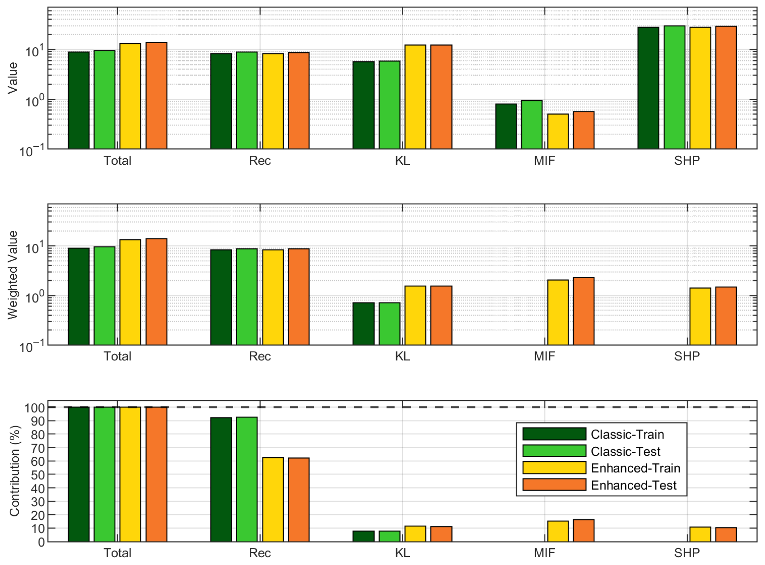
For this reason, the Decoder has been designed to embed an “hard” constraint that leads to the generation of Cholesky factors related to positive definite CSMs, which is another key aspect of the methodology presented. This guarantees the fundamental mathematical properties of synthetic CSMs and ensures that they are compatible with other techniques relying on them. Lastly, a custom Enhanced LF tailored to modal behaviour of structures has been developed to train the CNN-VAE model. Its implementation only requires the identification from the baseline dataset of the bands of analysis where the mode natural frequencies are located. The results demonstrated that this strategy improves the quality of synthetic data (Section 4.2) and that the latent variables become highly sensitive to structural dynamic changes and representative of the structural condition (Section 5.2).

The capability of CNN-VAE as generative model opens the possibility to different enhancements of vibration spectral data in the context of SHM. An example is the baseline balancing shown in Section 5.1, but any similar data augmentation approach can be easily integrated with the CNN-VAE model, such as the idea of “data-driven virtual baseline synthesis” suggested in [23]. One strength of the approach presented in this paper lies in the fact that traditional SHM methods based on frequency domain structural response can benefit from data synthesis. At the same time, the low-dimensional latent representation learnt by the Encoder enables other SHM approaches. Typical anomaly detection techniques can be implemented when only data related to an undamaged structure is initially available, such as One Class Support Vector Machine (OC-SVM) [64]. Moreover, monitoring data in the latent space can be integrated with classification techniques, for damage identification, or clustering techniques. Otherwise, more advanced anomaly detection strategies relying on the spectral reconstruction error [65] or custom novelty scores [59,66] are possible.

Practical implementations of an SHM strategy that makes use of this CNN-VAE model should take into account the computational costs and time requirements of different operations, on the basis of the estimates reported in Section 4. The heavy load is the initial training of the model on baseline data, but this is operated only once or when the baseline is updated. The generation of synthetic data for the purpose of implementing data augmentation and enhancement techniques combined with SHM approaches is significantly less computational resource-intensive. Typically, this is not a real-time operation, but the latent space monitoring can also be implemented in near-real-time. Indeed, encoding a CSM into latent space takes a fraction of a second. Therefore, the time to obtain the monitoring latent features is dominated by the measurement time required and the computation time required to estimate the CSM.

Other potential applications involve combining insights into structural behaviour derived from both simulation and experimental measurements. In fact, simulations can provide information about the structural behaviour under various configurations and conditions by means of parametric analyses, while experimental tests can reveal the gap between the complexity of a real structure that is not adequately represented by a finite element model. This typically happens with complex structures due to complex geometries and materials (e.g., anisotropy and non-linearity), as it is common for aerospace applications [67] and others. In such cases, the CNN-VAE model could be trained using frequency domain data from both worlds and merging the knowledge in a unique surrogate model.

7. Conclusions

The study successfully demonstrated the effectiveness of the CNN-VAE architecture designed specifically for structural vibration data in the frequency domain with the purpose of SHM technique enhancement. The use of Cholesky factorisation for handling CSMs has proved to be an advantageous choice, as well as the introduction of the Enhanced LF for model training, revealed to be crucial in improving the sensitivity to modal characteristics. The results obtained in the laboratory case study demonstrated the effectiveness of the CNN-VAE model in its dual use. The features learnt from spectral data can be used to implement an effective SHM strategy. Concurrently, the CNN-VAE serves as a powerful generative tool for producing realistic synthetic data, thus making it possible for it to be integrated into traditional SHM approaches based on frequency domain data by means of baseline augmentation strategies or similar.

The proposed framework offers a practical solution for improving vibration-based SHM systems, since the model does not have particularly limiting requirements in terms of number of vibration sensors and structural characteristics; hence, it is suitable for different type of structures, such as buildings, bridges, and aerospace structures, among others. This CNN-VAE model is already compliant with measuring 3D vibration response, since these are simply additional sensors; therefore, this extension is straightforward. Moreover, the very same architecture of the CNN-VAE is also compatible with other types of frequency domain data, such as frequency response functions or transmissibilities.

Future works will focus on the extension of this model in terms of its applications and architecture. A finer characterisation of damage evolution over monitoring could be useful to understand the fine sensitivity of the model to gradual changes in structure dynamics. A possible direction of improvement for the current model is the shift to the paradigm of Conditioned VAE, where measurements of EO factors are provided to the Decoder, which becomes aware of the conditions of that specific input, thus making the synthesis more controllable.