Dual-Tensor Constrained Multi-View Subspace Clustering

Abstract

Existing multi-view clustering approaches based on matrix factorization often fail to jointly capture global high-order correlations and local view-specific characteristics, and they typically suffer from instability in generating final clustering labels. To overcome these limitations, this paper presents a multi-view subspace clustering method termed dual-tensor constrained multi-view subspace clustering (DTCMVSC). Specifically, for each view, we learn an independent latent representation matrix, a projection matrix, and a basis matrix. The latent representations and projection matrices are stacked into third-order tensors, upon which tensor nuclear norm regularization is imposed to simultaneously exploit consensus structures and complementary information across views. Additionally, a consensus regularization term and adaptive view weights are introduced to align the latent representations of different views toward a unified consensus subspace. The resulting optimization problem is efficiently solved under the ADMM framework, after which a similarity matrix is constructed from the consensus representation and spectral clustering is performed to obtain the final labels. Experimental evaluations on six benchmark datasets demonstrate the superiority of DTCMVSC. Specifically, it achieves an ACC of 86.10% on CMU and an NMI of 94.17% on ORL, surpassing even the lowest-performing state-of-the-art baselines by 63.08 and 18.53 percentage points, respectively.

1. Introduction

Multi-view data consist of descriptions of the same object originating from different sources [1,2,3]. Due to variations in acquisition perspectives, attribute definitions, and input–output modalities, each view often captures different characteristics of the object, exhibiting significant diversity and complementarity. Although multi-view data are abundant in the real world, they most lack manual annotations. Therefore, how to effectively utilize such unlabeled data for object clustering, especially through unsupervised learning based on multi-view clustering techniques, has become a prominent research direction [4,5,6,7,8].

Existing multi-view clustering methods are diverse, among which subspace clustering, as an important approach in multi-view clustering algorithms, has consistently attracted significant attention [9,10,11,12,13]. Its core idea is to reveal the intrinsic correlations and differences among multi-view data by mining the latent structures of data in different subspaces. Within the subspace clustering framework, matrix factorization-based methods have become a key technique for multi-view subspace clustering due to their algorithmic simplicity and excellent interpretability [14,15,16,17,18]. Researchers have proposed various improvement strategies from different perspectives: Yang et al. [19] enhance clustering efficiency on large-scale data through consensus graph matrix factorization; Li et al. [20] leverage partial label information in semi-supervised scenarios to boost discriminative power; Zheng et al. [21] integrate matrix factorization and K-means into a unified framework to achieve mutual enhancement. However, these methods either rely on the shared matrix assumption while neglecting view-specificity [19,20], or they are constrained by the spherical cluster assumption of K-means, making it difficult to handle complex data distributions [21], thus still exhibiting limitations in multi-view subspace clustering.

To further improve performance, researchers have attempted to use the decomposed matrices as low-dimensional latent representations and combine them with spectral clustering for unsupervised data discrimination. Wang et al. [22] employ tensor Schatten p-norm regularization to mine multi-view complementary information and spatial structures; Zeng et al. [23] simultaneously capture consistency and complementarity across views via hypergraph regularization and orthogonal diversity constraints. Both methods apply spectral clustering to the learned low-dimensional representations to obtain the final clustering results. This strategy offers several advantages: First, spectral clustering constructs an adaptive affinity matrix (e.g., using a Gaussian kernel function) to capture local neighborhood relationships among data points rather than relying on a global shared matrix structure, thereby better preserving the diversity across different views. Second, spectral clustering maps the data into a low-dimensional space via spectral embedding and performs clustering using the eigenvectors of the Laplacian matrix, which naturally suits non-convex datasets and complex manifold structures, effectively overcoming K-means’ dependence on spherical clusters. Furthermore, directly feeding the low-dimensional representations obtained from matrix factorization into spectral clustering enables the synergistic optimization of representation learning and clustering objectives, avoiding error accumulation.

Although these methods have achieved significant progress, they still suffer from the following limitations. (1) Tensor regularization is applied to only a single matrix [22]. To better learn features, existing multi-view clustering algorithms based on matrix factorization often employ more than two factor matrices, yet imposing tensor regularization on only one matrix fails to simultaneously model the joint structure of the representation matrix and the projection matrix. (2) Graph-based regularization is unfriendly to non-graph data. When constructing graph topologies for non-graph structured data, such methods are highly sensitive to the parameters of various similarity computation functions [23], making it difficult to scale to the vast majority of real-world multi-view data. (3) The low-dimensional embedding representations learned in the representation learning stage are not fully utilized. The learned low-dimensional embeddings, often obtained through elaborate designs, are typically fed into simple k-means or direct truncation methods to generate clustering labels, leading to unstable clustering results that depend heavily on the initialization of the algorithm.

These observations lead to the following research question: Can simultaneously imposing tensor nuclear norm regularization on multiple factor matrices, rather than a single one, more effectively capture cross-view consensus while preserving view-specific information, and can this be integrated with spectral clustering in a way that yields stable and discriminative labels? We hypothesize that the latent representation matrix and the projection matrix encode complementary aspects of the multi-view structure—the former capturing sample-level consensus and the latter reflecting feature-level relationships—and that jointly constraining both via tensor nuclear norm regularization can exploit high-order correlations that a single constraint cannot access. To this end, this paper proposes a multi-view clustering method based on double tensor-constrained three-factor matrix factorization. The method imposes tensor nuclear norm regularization on both the latent representation matrix and the projection matrix simultaneously, effectively mining global consistency information across views. Meanwhile, it explicitly preserves the unique features of each view in the basis matrix as complementary enhancements. Furthermore, the algorithm introduces an adaptive view weighting mechanism to automatically identify and fuse the view combination that contributes most to clustering. Finally, the learned basis matrix is used as the low-dimensional latent representation of the data, and spectral clustering is employed to derive the final clustering partition.

The main contributions of this paper are as follows:

• A novel three-factor matrix factorization framework with double tensor regularization is proposed. To jointly capture global consistency and local specificity across views, double tensor nuclear norm constraints are imposed on the factor matrices, enabling low-dimensional consensus mining while preserving view-unique features.
• A collaborative mechanism integrating consistency constraints and spectral clustering is designed. A consistency regularization term is embedded into the decomposition, and a high-fidelity similarity matrix is built via Euclidean distance. Seamlessly linking the latent representation with spectral clustering enhances the robustness and discriminability of clustering labels.
• State-of-the-art performance is achieved on multiple benchmarks. Extensive experiments on six real-world multi-view datasets show that the proposed method significantly outperforms existing algorithms across key metrics, validating its effectiveness and generalization.

The remainder of this paper is organized as follows. Section 2 reviews related work on multi-view subspace clustering based on matrix factorization, spectral clustering label generation methods, and tensor nuclear norm regularization, and concludes with a summary and positioning of the proposed method. Section 3 presents the proposed DTCMVSC method, including the notation, motivation, objective function formulation, and the ADMM-based optimization procedure. Section 4 reports experimental results on six benchmark datasets, covering performance comparison, ablation studies, parameter sensitivity analysis, convergence analysis, visualization, and time complexity analysis. Section 5 concludes the paper and discusses future research directions.

2. Related Work

2.1. Multi-View Subspace Clustering Based on Matrix Factorization

Multi-view subspace clustering integrates information from multiple views to mine the latent subspace structure of data. The basic form of matrix factorization can be expressed as shown below:

$$\underset{Q,P}{\min }{\parallel X-QP\parallel }_F^2+\lambda \parallel \mathrm{\Theta }\parallel ,$$

(1)

where $Q\in {\mathbb{R}}^{n\times k}$ is the basis matrix, $P\in {\mathbb{R}}^{k\times d}$ is the representation matrix, and $\mathrm{\Theta }$ denotes a regularization constraint.

Existing methods can be roughly divided into three categories: shared matrix models, aligned matrix models, and graph-regularized models.

For shared matrix models, Zhang and Lu [24] proposed TMMVC, which achieves alignment and fusion via multi-dimensional embeddings and view-specific rotation matrices, and it introduces the tensor Schatten-p norm to enhance sparsity and low rankness. However, tensor regularization and repeated decomposition operations increase computational cost and lead to slow convergence.

For aligned matrix models, Zhang et al. [25] proposed ODNMF, which reduces feature redundancy through basis matrix orthogonalization, introduces a diversity enhancement term to explore complementary information across views, and constructs graph regularization for each view. Nevertheless, strict orthogonal constraints may oversimplify the complex relationships among data features, impairing the model’s expressiveness.

For graph-regularized models, Liang et al. [26] proposed LGGMF for incomplete multi-view clustering, which constructs a consensus graph from the common representation via a local graph generation strategy. However, its time complexity is $O\left(n^3\right)$, limiting scalability to large-scale data, and it lacks robustness to view-level noise.

Deep matrix factorization methods have gained attention in recent years. Khalafaoui et al. [27] proposed DMFAW, combining weighted deep Semi-NMF with PI step-size control to achieve dynamic feature selection and adaptive parameter update. However, this method only handles feature-level noise and does not address robustness to view-level noise.

From the perspective of subspace clustering, Luo et al. [6] proposed CSMSC, which decomposes the self-representation matrix into a shared consistent representation C and view-specific representations $D^{\left(v\right)}$, i.e., $Z^{\left(v\right)}=C+f{D}^{\left(v\right)}$, imposing a nuclear norm on C and a Frobenius norm on $D^{\left(v\right)}$. The self-representation matrix has size $O\left(n^2\right)$, leading to a complexity of $O\left(n^3\right)$, and the representation learning for each view is independent, lacking high-order collaborative modeling.

Chen et al. [28] proposed MvSCGE, which preserves the grouping effect of subspace representations via graph Laplacian regularization while introducing cross-view consistency regularization. It also relies on an $O\left(n^3\right)$ self-representation matrix, making it difficult to scale to large data.

To handle large-scale data, Bian et al. [29] proposed AFMC, which learns binary representations via angular reconstruction error minimization and discrete ridge regression, achieving linear time complexity. However, binarization causes information loss, and the explicit modeling of high-order correlations across views is lacking.

To enhance nonlinear modeling capability, Deng et al. [30] proposed SNDRMvC, which decouples the SNMF update into element-wise SGD and constructs a deep network, but it is sensitive to dataset size and prone to overfitting on small data. Cui et al. [31] proposed N3MF, which parameterizes part of the NMF iteration as network layers, balancing interpretability and flexibility, though scalability on ultra-large-scale data still requires verification.

For incomplete multi-view clustering, Wen et al. [32] proposed GreatF, introducing adaptive feature weighting and graph embedding consensus learning, but the weighting only applies to raw features and does not extend to low-dimensional representations. Dong et al. [33] proposed CRLSNMF, introducing center graph regularization and $l_{2,log}$ norm to enhance sparsity, yet its computational complexity grows quadratically with the number of samples, leaving room for efficiency improvement.

The above methods demonstrate that matrix factorization can effectively fuse multi-view information, but most methods constrain only a single factor matrix, making it difficult to fully model high-order collaborative relationships across views. Inspired by this, we adopt a three-factor matrix factorization framework that separates the consensus representation of samples from view projections, and we introduce double tensor nuclear norms to simultaneously constrain both matrices, thereby more comprehensively mining cross-view structures.

2.2. Spectral Clustering Label Generation Methods

A common paradigm is to first learn a shared low-dimensional representation Q via matrix factorization, then construct a similarity matrix and feed it into spectral clustering to obtain discrete labels. Specifically, given multi-view data ${\left\{X^{\left(v\right)}\right\}}_{v=1}^m$, we solve

$$\underset{Q,{\left\{P^{\left(v\right)}\right\}}_{v=1}^m}{\min }{\displaystyle \sum _{v=1}^m}{\parallel X^{\left(v\right)}-Q{P}^{\left(v\right)}\parallel }_F^2+\lambda \mathcal{R}(Q,\left\{P^{\left(v\right)}\right\}),$$

(2)

where $Q\in {\mathbb{R}}^{n\times k}$ is the consensus representation and $P^{\left(v\right)}\in {\mathbb{R}}^{k\times d_v}$ is the basis matrix. Subsequently, a similarity matrix A (e.g., Gaussian kernel or k-NN graph) is constructed based on Q and fed into spectral clustering to obtain labels.

This strategy has been widely adopted. For example, Wang et al. [22] proposed tensorized multi-view clustering based on orthogonal semi-nonnegative three-factor decomposition and performed spectral clustering on the consensus matrix. However, this method still relies on a full similarity matrix, incurring high computational cost. Wang et al. [34] proposed FPMVS-CAG, which jointly optimizes anchor selection and subgraph construction and performs spectral clustering on the anchor graph with linear complexity. Nevertheless, anchor quality significantly affects performance, and robustness to noise is lacking.

Anchor-based large-scale methods further enrich this line. Liu et al. [35] proposed MVC-WA, introducing adaptive anchor weighting but ignoring redundancy among anchors. Chen et al. [36] proposed AGLDR, which filters Gaussian and Laplacian noise during anchor graph learning, yet the low-rank constraint only applies to the consensus anchor graph, failing to simultaneously constrain multiple key matrices. Ma et al. [37] proposed 3AMVC, which automatically determines and aligns the number of anchors, but anchor selection and graph construction remain relatively independent.

To overcome the information loss of two-stage methods, some studies unify spectral embedding and discrete label learning. Yang et al. [38] proposed TLMSC, utilizing triplets and fast sparse spectral clustering, but triplet generation depends on predefined similarities and hard negative mining requires class-balance assumptions. Zhong and Pun [39] proposed SMSC, which unifies adaptive weighting, consensus graph learning, spectral embedding, and spectral rotation to directly output labels, yet the alternating optimization of graph learning and spectral embedding leads to slow convergence. Yang et al. [40] proposed SMMSC, adopting a min–max framework to maximize intra-cluster variance, but it requires the manual tuning of multiple parameters and is sensitive to noise.

The two-stage strategy of “matrix factorization/anchor graph + spectral clustering” has clear advantages in robustness and generalization: low-dimensional representations filter noise, while spectral clustering adaptively captures global structure. Therefore, this paper follows this technical route, feeding the learned consensus representation Q into spectral clustering to obtain final labels, balancing efficiency and stability.

2.3. Regularization Term Based on Tensor Nuclear Norm

The tensor nuclear norm (TNN) is based on t-SVD. Given a third-order tensor $\mathcal{X}\in {\mathbb{R}}^{n_1\times n_2\times n_3}$, its t-SVD is

$$\mathcal{X}=\mathcal{U}\ast \mathcal{S}\ast {\mathcal{V}}^{\top },$$

(3)

where $\mathcal{U}$ and $\mathcal{V}$ are orthogonal, and $\mathcal{S}$ is an f-diagonal tensor. The TNN is defined as

$${\parallel \mathcal{X}\parallel }_{★}={\displaystyle \frac{1}{n_3}}{\displaystyle \sum _{i=1}^{n_3}}{\parallel {\overline{\mathcal{X}}}^{\left(i\right)}\parallel }_{★}={\displaystyle \frac{1}{n_3}}{\displaystyle \sum _{i=1}^{n_3}}{\displaystyle \sum _{j=1}^{\min (n_1,n_2)}}{\sigma }_j^{\left(i\right)},$$

(4)

where ${\overline{\mathcal{X}}}^{\left(i\right)}$ is the i-th frontal slice after the Fourier transform.

TNN is used in multi-view clustering to capture high-order cross-view correlations. Shi et al. [41] employed TNN to constrain a graph tensor in CSTGL. Zhang et al. [42] proposed a weighted arctangent coupled TNN. Luo et al. [43] introduced a tensor log-determinant function. However, these methods typically impose constraints on only a single tensor (e.g., the self-representation coefficient), failing to fully exploit the multi-dimensional structure of multi-view data.

Most existing methods apply TNN to only a single factor matrix. Wang et al. [44] proposed TPCH, stacking the projection matrix and hash codes into a tensor and imposing an enhanced TNN (ETNN), but this remains a binary representation method where quantization loss limits representation accuracy. Li et al. [45] proposed tensorized discrete multi-view spectral clustering, applying TNN to the spectral embedding tensor without simultaneously constraining the projection matrix, resulting in incomplete information mining.

To further improve scalability, Long et al. [46] proposed TLRLF4MVC, simultaneously imposing TNN and a tensor low-frequency component (TLFC) operator to efficiently capture high-order inter-view correlations and intra-view smoothness. However, the low-frequency component relies on graph Fourier transform, requiring the pre-construction of a global similarity graph, which increases preprocessing overhead. For incomplete multi-view clustering, Shen et al. [47] proposed RIMC, utilizing marginalized denoising and low-rank priors along three dimensions for tensor completion, but the complexity is as high as $O\left(n^{3}V\right)$, making it difficult to apply to ultra-large-scale data. Huang et al. [48] proposed LTLPDM, applying TNN to the subspace representation tensor while jointly learning the projection matrix and projection distance metric, but each subproblem requires solving Sylvester equations, leading to high per-iteration complexity.

The above works validate the effectiveness of TNN in mining high-order multi-view structures, but most constrain only a single matrix (e.g., self-representation coefficients, spectral embeddings, or subspace representations). Inspired by this, this paper proposes a double tensor nuclear norm regularization strategy, imposing low-rank constraints on both the latent representation matrix and the projection matrix simultaneously, capturing cross-view consensus information from both key matrices via t-SVD, thereby achieving more comprehensive modeling of high-order multi-view structures.

2.4. Summary and Positioning

To better situate the proposed method within the existing literature,

Table 1. Comparison of design choices: prior methods vs. DTCMVSC.

Design Dimension	Limitations of Prior Methods	DTCMVSC Strategy
Tensor regularization scope	Most tensor-based methods impose tensor nuclear norm on only a single matrix (e.g., representation or embedding), leaving the projection structure unconstrained.	Applies double tensor nuclear norm regularization on both the latent representation tensor $\mathcal{W}$ and the projection tensor $\mathcal{S}$, jointly capturing high-order correlations from two complementary factor matrices.
Cross-view alignment mechanism	Shared-matrix models assume a common representation, overlooking view-specific variations. Graph-based methods rely on pre-constructed similarity graphs, whose quality is parameter-sensitive for non-graph data.	Introduces a consensus regularization term with adaptive view weights, aligning latent representations toward a unified subspace without requiring graph topology construction.
Label generation strategy	Several methods feed learned embeddings into simple k-means or direct truncation, which can produce unstable results sensitive to initialization.	Constructs a similarity matrix from the consensus representation via Euclidean distance and employs spectral clustering on the normalized Laplacian, yielding stable and discriminative final labels.

summarizes the key design dimensions discussed above and contrasts the limitations of representative prior works with the corresponding strategies adopted in DTCMVSC.

As shown in Table 1, DTCMVSC addresses several open challenges in a unified framework: extending tensor regularization from a single matrix to dual matrices, replacing parameter-sensitive graph regularization with adaptive consensus alignment, and integrating spectral clustering for label stabilization. With this positioning, we now present the detailed formulation of the proposed method.

3. Method

3.1. Notation

In this subsection, we introduce the main symbols used throughout the paper. For ease of reference, the key notations are summarized in

Table 2. Main symbols and their descriptions.

Symbol	Description
$X_v$	v-th view data, $n\times d_v$
$W_v$	Latent representation, $n\times m$, $W_v^{\top }{W}_v=I_m$
$S_v$	Intermediate factor, $m\times k$, $S_v^{\top }{S}_v=I_k$
$H_v$	View-specific basis matrix, $k\times d_v$
$W^{\ast }$	Consensus matrix, $n\times m$
$\mathcal{W}$	Tensor from $\left\{W_v\right\}$, size $n\times m\times V$
$\mathcal{S}$	Tensor from $\left\{S_v\right\}$, size $m\times k\times V$
$\mathcal{J},\mathcal{K}$	Auxiliary tensors for $\mathcal{W}$, $\mathcal{S}$ in TNN
${\mathcal{Y}}_W,{\mathcal{Y}}_S$	Lagrange multipliers for $\mathcal{W}=\mathcal{J}$, $\mathcal{S}=\mathcal{K}$
$\alpha$	Number of columns of $W_v$, denoted by m
${\beta }_v$	Adaptive weight of v-th view
${\lambda }_1,{\lambda }_2,{\lambda }_3$	Regularization parameters
${\rho }_1,{\rho }_2$	ADMM penalty parameters ($\rho >0$)
${\parallel ·\parallel }_F$	Frobenius norm
${\parallel ·\parallel }_{\ast }$	Tensor nuclear norm (avg. of frontal slice SV sums in Fourier domain)
$\langle ·,·\rangle$	Frobenius inner product
$I_m,I_k$	Identity matrices

.

3.2. Motivation and Objective Function

Matrix factorization is a classic dimensionality reduction method. Compared with two-factor decomposition, three-factor matrix factorization has stronger latent feature learning and dimensionality reduction capabilities, and its basic form can be expressed as

$$X\approx WSH.$$

(5)

In multi-view scenarios, the data distributions of different views often differ significantly. If a unified consensus representation is directly used for all views, it is difficult to achieve ideal clustering performance when the differences between views are large. Therefore, learning a view-specific representation for each view is key to improving clustering performance. Accordingly, the following objective function can be constructed:

$$\begin{array}{cc}\hfill \underset{W_v,S_v,H_v}{\min }& {\displaystyle \sum _{v=1}^V}{\parallel X_v-W_v{S}_v{H}_v\parallel }_F^2\hfill \\ \hfill \mathrm{s}.\mathrm{t}.& W_v^{\top }{W}_v=I_m,S_v^{\top }{S}_v=I_k,\forall v.\hfill \end{array}$$

(6)

Imposing column-wise orthogonal constraints on $W_v$ and $S_v$ prevents the model from confusing samples from different classes into the same class during training, avoids the learned low-dimensional representation having a dimension lower than the actual number of clusters, and thus ensures the validity of clustering. No orthogonal constraint is imposed on $H_v$, because such a strong constraint may limit the model’s ability to learn features.

Traditional Laplacian graph regularization and ${\ell }_1$, ${\ell }_2$ norm regularization often fail to effectively utilize cross-view information. In contrast, tensor nuclear norm regularization fuses information from different views via Fourier transform, allowing the factor matrices of different views to learn from and enhance each other. In the three-factor decomposition framework, imposing tensor nuclear norm regularization only on the basis matrix $W_v$ often causes the optimization results of other matrices to be too scattered, which is not conducive to forming the final clustering objective. To this end, this paper proposes to impose tensor nuclear norm regularization on both $W_v$ and $S_v$, resulting in the following objective function:

$$\begin{array}{cc}\hfill \underset{W_v,S_v,H_v}{\min }& {\displaystyle \sum _{v=1}^V}\parallel X_v-W_v{S}_v{H}_v{\parallel }_F^2+{\lambda }_1{\parallel \mathcal{W}\parallel }_{\ast }+{\lambda }_2{\parallel \mathcal{S}\parallel }_{\ast }\hfill \\ \hfill \mathrm{s}.\mathrm{t}.& W_v^{\top }{W}_v=I_m,S_v^{\top }{S}_v=I_k,\forall v,\hfill \end{array}$$

(7)

where $\mathcal{W}$ is the tensor formed by stacking ${\left\{W_v\right\}}_{v=1}^V$ along the third dimension, and $\mathcal{S}$ is defined analogously.

To further exploit the learned factor matrices for generating better clustering results, we introduce a consensus regularization term on $W_v$ to align them toward a unified consensus matrix during training, and we assign adaptive weights to different views to better fuse multi-view information. The final objective function is defined as

$$\begin{array}{cc}\hfill \underset{W_v,S_v,H_v,W^{\ast }}{\min }& {\displaystyle \sum _{v=1}^V}{\beta }_v\left(\parallel X_v-W_v{S}_v{H}_v{\parallel }_F^2+{\displaystyle \frac{{\lambda }_3}{2}}{\parallel W_v-W^{\ast }\parallel }_F^2\right)\hfill \\ \hfill & +{\lambda }_1{\parallel \mathcal{W}\parallel }_{\ast }+{\lambda }_2{\parallel \mathcal{S}\parallel }_{\ast }\hfill \\ \hfill \mathrm{s}.\mathrm{t}.& W_v^{\top }{W}_v=I_m,S_v^{\top }{S}_v=I_k,\forall v,\hfill \end{array}$$

(8)

where ${\lambda }_1>0$, ${\lambda }_2>0$, ${\lambda }_3>0$ are regularization parameters, and ${\beta }_v>0$ is the adaptive weight for the v-th view.

After solving the above optimization, we obtain the consensus matrix $W^{\ast }$. To obtain the final clustering labels, we first perform row normalization on $W^{\ast }$; then, we construct a similarity matrix based on Euclidean distance:

$$A_{ij}={\displaystyle \frac{1}{1+\parallel {\mathbf{w}}_i^{\ast }-{\mathbf{w}}_j^{\ast }{\parallel }_2^2}},$$

(9)

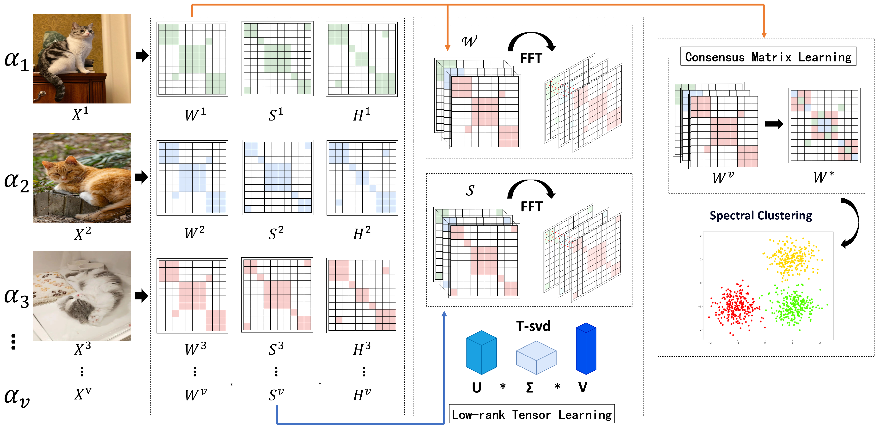
where ${\mathbf{w}}_i^{\ast }$ is the i-th row of $W^{\ast }$. After sparsifying and symmetrizing A using k-nearest neighbors, we construct the symmetric normalized Laplacian matrix $L=I-D^{-1/2}A{D}^{-1/2}$, where D is the degree matrix. The smallest $c+1$ eigenvectors of L are computed, the 2nd to $(c+1)$-th vectors are taken to form matrix F, and k-means clustering is performed on the rows of F to finally obtain the cluster label for each sample. This method leverages the global structural information contained in $W^{\ast }$ and achieves efficient and stable cluster partitioning via spectral clustering under Euclidean distance (see Figure 1).

3.3. Optimization Derivation

We adopt the ADMM optimization method [49], which has been widely employed in multi-view clustering due to its rigorous convergence guarantees for problems with multiple coupled variables. First, we construct the augmented Lagrangian function; then, we adopt an alternating minimization strategy to update each variable sequentially.

$$\begin{array}{cc}\hfill \mathcal{L}=& {\displaystyle \sum _{v=1}^V}{\beta }_v\left(\parallel X_v-W_v{S}_v{H}_v{\parallel }_F^2+{\displaystyle \frac{{\lambda }_3}{2}}{\parallel W_v-W^{\ast }\parallel }_F^2\right)\hfill \\ \hfill & +{\lambda }_1{\parallel \mathcal{J}\parallel }_{\ast }+{\lambda }_2{\parallel \mathcal{K}\parallel }_{\ast }\hfill \\ \hfill & +\langle {\mathcal{Y}}_W,\mathcal{W}-\mathcal{J}\rangle +{\displaystyle \frac{{\rho }_1}{2}}{\parallel \mathcal{W}-\mathcal{J}\parallel }_F^2\hfill \\ \hfill & +\langle {\mathcal{Y}}_S,\mathcal{S}-\mathcal{K}\rangle +{\displaystyle \frac{{\rho }_2}{2}}{\parallel \mathcal{S}-\mathcal{K}\parallel }_F^2,\hfill \end{array}$$

(10)

where $\mathcal{J}$ and $\mathcal{K}$ are auxiliary tensor variables for decoupling the tensor nuclear norm; ${\mathcal{Y}}_W$ and ${\mathcal{Y}}_S$ are Lagrange multiplier tensors for the equality constraints $\mathcal{W}=\mathcal{J}$ and $\mathcal{S}=\mathcal{K}$; ${\rho }_1,{\rho }_2>0$ are ADMM penalty parameters; and ${\beta }_v$ is the view weight, which simultaneously controls both the reconstruction error term and the consensus term in the adaptive mode. For brevity, we use ${\beta }_v$ uniformly in the following.

The update steps in the $(t+1)$-th iteration of ADMM are as follows.

• Update $W_v$ (independently for each view)

$$W_v^{t+1}=\arg \underset{W_v^{\top }{W}_v=I_m}{\min }{\beta }_v\parallel X_v-W_v{S}_v^t{H}_v^t{\parallel }_F^2+{\displaystyle \frac{{\lambda }_3{\beta }_v}{2}}\parallel W_v-W^{\ast t}{\parallel }_F^2+{\displaystyle \frac{{\rho }_1}{2}}\parallel W_v-J_v^t+{\displaystyle \frac{1}{{\rho }_1}}{Y}_{W,v}^t{\parallel }_F^2.$$

Ignoring constant terms independent of $W_v$, the problem is equivalent to

$$W_v^{t+1}=\arg \underset{W_v^{\top }{W}_v=I_m}{\min }{\parallel W_v-M_v^t\parallel }_F^2,$$

where

$$M_v^t={\beta }_v{X}_v{\left(H_v^t\right)}^{\top }{\left(S_v^t\right)}^{\top }+{\displaystyle \frac{{\lambda }_3{\beta }_v}{2}}{W}^{\ast t}+{\displaystyle \frac{{\rho }_1}{2}}{J}_v^t-{\displaystyle \frac{1}{2}}{Y}_{W,v}^t.$$

This is an orthogonal Procrustes problem, whose optimal solution is obtained via the singular value decomposition of $M_v^t$: let $M_v^t=U\mathrm{\Sigma }{V}^{\top }$, then $W_v^{t+1}=U{V}^{\top }$.

2.

Update consensus matrix $W^{\ast }$

$$W^{\ast t+1}=\arg \underset{W^{\ast }}{\min }{\displaystyle \sum _{v=1}^V}{\displaystyle \frac{{\lambda }_3{\beta }_v}{2}}{\parallel W_v^{t+1}-W^{\ast }\parallel }_F^2={\displaystyle \frac{{\sum }_{v=1}^V{\beta }_v{W}_v^{t+1}}{{\sum }_{v=1}^V{\beta }_v}}.$$

3.

Update $S_v$ (independently for each view)

$$S_v^{t+1}=\arg \underset{S_v^{\top }{S}_v=I_k}{\min }{\beta }_v\parallel X_v-W_v^{t+1}{S}_v{H}_v^t{\parallel }_F^2+{\displaystyle \frac{{\rho }_2}{2}}\parallel S_v-K_v^t+{\displaystyle \frac{1}{{\rho }_2}}{Y}_{S,v}^t{\parallel }_F^2.$$

After ignoring constant terms, the problem reduces to

$$S_v^{t+1}=\arg \underset{S_v^{\top }{S}_v=I_k}{\min }{\parallel S_v-N_v^t\parallel }_F^2,$$

where

$$N_v^t={\beta }_v{\left(W_v^{t+1}\right)}^{\top }{X}_v{\left(H_v^t\right)}^{\top }+{\displaystyle \frac{{\rho }_2}{2}}{K}_v^t-{\displaystyle \frac{1}{2}}{Y}_{S,v}^t.$$

Again, this is an orthogonal Procrustes problem solved via SVD: let $N_v^t=U\mathrm{\Sigma }{V}^{\top }$, then $S_v^{t+1}=U{V}^{\top }$.

4.

Update $H_v$ (unconstrained)

$$H_v^{t+1}=\arg \underset{H_v}{\min }{\beta }_v{\parallel X_v-W_v^{t+1}{S}_v^{t+1}{H}_v\parallel }_F^2={\left(S_v^{t+1}\right)}^{\top }{\left(W_v^{t+1}\right)}^{\top }{X}_v.$$

5.

Update auxiliary tensor $\mathcal{J}$ (tensor nuclear norm for $\mathcal{W}$)

$${\mathcal{J}}^{t+1}=\arg \underset{\mathcal{J}}{\min }{\displaystyle \frac{{\lambda }_1}{{\rho }_1}}{\parallel \mathcal{J}\parallel }_{\ast }+{\displaystyle \frac{1}{2}}\parallel \mathcal{J}-({\mathcal{W}}^{t+1}+{\displaystyle \frac{1}{{\rho }_1}}{\mathcal{Y}}_W^t){\parallel }_F^2.$$

This proximal operator is implemented via singular value thresholding in the Fourier domain. Let

$$\tilde{\mathcal{M}}={\mathcal{W}}^{t+1}+{\displaystyle \frac{1}{{\rho }_1}}{\mathcal{Y}}_W^t,$$

and perform the fast Fourier transform along the third dimension of $\tilde{\mathcal{M}}$ to obtain the frequency-domain tensor $\widehat{\mathcal{M}}$. For each frequency $l=1,\dots ,\lceil (V+1)/2\rceil$, compute

$${\widehat{\mathcal{J}}}^{\left(l\right)}={\mathcal{T}}_{{\displaystyle \frac{{\lambda }_1}{{\rho }_1}}}\left({\widehat{\mathcal{M}}}^{\left(l\right)}\right),$$

where ${\mathcal{T}}_{\tau }(·)$ is the singular value soft-thresholding operator:

$${\mathcal{T}}_{\tau }\left(M\right)=Umax(\mathrm{\Sigma }-\tau I,0)V^{\top },M=U\mathrm{\Sigma }{V}^{\top }.$$

Finally, apply the inverse Fourier transform to obtain ${\mathcal{J}}^{t+1}$.

6.

Update auxiliary tensor $\mathcal{K}$ (tensor nuclear norm for $\mathcal{S}$)

Similarly,

$${\mathcal{K}}^{t+1}=\arg \underset{\mathcal{K}}{\min }{\displaystyle \frac{{\lambda }_2}{{\rho }_2}}{\parallel \mathcal{K}\parallel }_{\ast }+{\displaystyle \frac{1}{2}}\parallel \mathcal{K}-({\mathcal{S}}^{t+1}+{\displaystyle \frac{1}{{\rho }_2}}{\mathcal{Y}}_S^t){\parallel }_F^2,$$

also solved by singular value thresholding in the Fourier domain.

7.

Update lagrange multipliers ${\mathcal{Y}}_W$, ${\mathcal{Y}}_S$

$${\mathcal{Y}}_W^{t+1}={\mathcal{Y}}_W^t+{\rho }_1({\mathcal{W}}^{t+1}-{\mathcal{J}}^{t+1}),$$

$${\mathcal{Y}}_S^{t+1}={\mathcal{Y}}_S^t+{\rho }_2({\mathcal{S}}^{t+1}-{\mathcal{K}}^{t+1}).$$

8.

Adaptive adjustment of ${\rho }_1$, ${\rho }_2$

Define the primal and dual residuals after the t-th iteration:

$$\begin{array}{cc}\hfill r_{\mathrm{pri},1}^{\left(t\right)}& =\parallel {\mathcal{W}}^t-{\mathcal{J}}^t{\parallel }_F,\hfill \\ \hfill r_{\mathrm{dual},1}^{\left(t\right)}& ={\rho }_1^{\left(t\right)}{\parallel {\mathcal{J}}^t-{\mathcal{J}}^{t-1}\parallel }_F,\hfill \\ \hfill r_{\mathrm{pri},2}^{\left(t\right)}& =\parallel {\mathcal{S}}^t-{\mathcal{K}}^t{\parallel }_F,\hfill \\ \hfill r_{\mathrm{dual},2}^{\left(t\right)}& ={\rho }_2^{\left(t\right)}{\parallel {\mathcal{K}}^t-{\mathcal{K}}^{t-1}\parallel }_F.\hfill \end{array}$$

A check is performed every $T=10$ iterations, and it becomes effective starting from the 20th iteration. The specific rules are as follows:

• For ${\rho }_1$: If the primal residual is significantly larger than the dual residual, i.e.,

  $$r_{\mathrm{pri},1}^{\left(t\right)}>\mu r_{\mathrm{dual},1}^{\left(t\right)},\mu =10,$$

  then increase the penalty parameter:

  $${\rho }_1^{(t+1)}=\min \left({\rho }_{\mathrm{inc}}·{\rho }_1^{\left(t\right)},{\rho }_{\max }\right),$$

  where ${\rho }_{\mathrm{inc}}=1.1$ is the increase factor and ${\rho }_{\max }$ is a preset upper bound. To maintain the consistency of the multipliers, the Lagrange multiplier tensor is scaled accordingly:

  $${\mathcal{Y}}_W^{(t+1)}={\displaystyle \frac{{\rho }_1^{(t+1)}}{{\rho }_1^{\left(t\right)}}}{\mathcal{Y}}_W^{\left(t\right)}.$$
• For ${\rho }_2$: Similarly, if

  $$r_{\mathrm{pri},2}^{\left(t\right)}>\mu r_{\mathrm{dual},2}^{\left(t\right)},$$

  then

  $${\rho }_2^{(t+1)}=\min \left({\rho }_{\mathrm{inc}}·{\rho }_2^{\left(t\right)},{\rho }_{\max }\right),{\mathcal{Y}}_S^{(t+1)}={\displaystyle \frac{{\rho }_2^{(t+1)}}{{\rho }_2^{\left(t\right)}}}{\mathcal{Y}}_S^{\left(t\right)}.$$

9.

Adaptive view weight update

To enhance the model’s robustness to noisy views, an adaptive weight update strategy based on reconstruction error is introduced. Suppose after the t-th iteration, the reconstruction error for each view is

$$e_v^{\left(t\right)}={\parallel X_v-W_v^{\left(t\right)}{S}_v^{\left(t\right)}{H}_v^{\left(t\right)}\parallel }_F^2,v=1,\dots ,V.$$

First, normalize the errors to eliminate scale effects:

$${\tilde{e}}_v^{\left(t\right)}={\displaystyle \frac{e_v^{\left(t\right)}}{{max}_{v^{\prime }}{e}_{v^{\prime }}^{\left(t\right)}}}.$$

The weight update formula is

$${\beta }_v^{(t+1)}=V·{\displaystyle \frac{exp\left(-\eta {\tilde{e}}_v^{\left(t\right)}\right)+ϵ}{{\sum }_{v^{\prime }=1}^V\left(exp\left(-\eta {\tilde{e}}_{v^{\prime }}^{\left(t\right)}\right)+ϵ\right)}},$$

where $\eta >0$ is a sensitivity hyperparameter and $ϵ={10}^{-6}$ is a small smoothing constant to prevent zero weights. This update assigns higher weights to views with smaller reconstruction errors, thereby suppressing the interference of low-quality views. Weight updates are performed alternately with ADMM variable updates every $T_{\mathrm{weight}}=10$ iterations (see Algorithm 1).

Algorithm 1: Dual-Tensor Constrained Multi-View Subspace Clustering

4. Experiments

4.1. Experimental Datasets

We conduct experiments on six benchmark datasets: 100 leaves, 3 sources, CMU, MSRCV, ORL, and WebKB, covering image, text, and video data:

• 100 leaves: contains 100 plant leaf species, each sample is described by three feature views: shape, texture, and margin.
• 3 sources: a multi-view text dataset consisting of the same news stories from three sources: BBC, Guardian, and Telegraph, each source as one view.
• CMU: a face image dataset containing face photos under different poses, illuminations, and expressions, where different conditions are often treated as multiple views.
• MSRCV: a video action recognition dataset containing various daily action videos, where features such as appearance and optical flow are commonly used to construct multiple views.
• ORL: contains grayscale face images of 40 individuals, 10 images per person, covering different lighting and expression variations.
• WebKB: a web page classification dataset, utilizing web page text content and hyperlink structure as two complementary views.

Among them, WebKB and 3 sources are heterogeneous datasets due to inherent differences in modalities or sources (see

Table 3. Statistics of multi-view datasets.

Dataset	Samples	Classes	Views	Feature Dimensions
3 sources	169	6	3	3560, 3631, 3068
WebKB	203	4	3	1703, 230, 230
MSRCV	210	7	6	1302, 48, 512, 100, 256, 210
ORL	400	40	3	4096, 3304, 6750
100 leaves	1600	100	3	64, 64, 64
CMU	2856	68	3	30, 30, 30

).

4.2. Experimental Environment

All experiments are conducted on a laptop equipped with an 11th Gen Intel Core i9-11980HK processor (2.60 GHz base frequency, 3.30 GHz boost) and 64 GB of RAM (Santa Clara, CA, USA), running a 64-bit Windows operating system.

4.3. Introduction to Compared Methods

• AFMC [29]. This method proposes a large-scale multi-view clustering approach that jointly optimizes the angular reconstruction error to preserve global similarity and introduces discrete ridge regression with fused similarity to retain local manifold structure, thereby learning a compact and discriminative shared binary representation in Hamming space.
• MvSCGE [28]. This method proposes a multi-view subspace clustering approach that simultaneously learns view-specific subspace representations and introduces smooth regularization to explicitly preserve intra-subspace locality (i.e., the grouping effect) along with cross-view consistency constraints, thereby obtaining stable subspaces and consistent clustering results within a unified optimization framework.
• TPCH [44]. This method proposes a multi-view clustering approach that stacks multiple projection matrices and hash codes into a tensor and employs an enhanced tensor nuclear norm to capture high-order interactions, thereby learning a more compact and discriminative binary representation to improve multi-view clustering performance.
• CSMSC [6]. This method proposes a consistency- and specificity-aware multi-view subspace clustering framework, which innovatively decomposes the self-representation coefficients of each view explicitly into a shared consistent component and a view-specific component. Through a joint optimization strategy, it effectively integrates the consensus structure across views while preserving view-specific diversity, thereby significantly improving the robustness and accuracy of clustering results.
• MVC-WA [35]. This method proposes an efficient and robust clustering framework that significantly reduces computational complexity by constructing a sample-anchor bipartite graph, and it introduces an adaptive view weighting mechanism to distinguish the reliability of different views. Thus, it effectively integrates consensus information across views while suppressing the interference of noisy views, improving clustering performance in large-scale scenarios.
• AGLDR [36]. This method proposes a robust anchor graph learning approach with dual denoising capabilities. It jointly minimizes the Frobenius norm and the $L_{2,1}$ norm to specifically eliminate Gaussian noise and Laplacian noise in the data, respectively, and it learns a consensus anchor graph under low-rank constraints, thereby significantly improving the accuracy and robustness of multi-view clustering in complex noisy environments.
• 3AMVC [37]. This method proposes an automatic and aligned anchor learning strategy. It innovatively introduces hierarchical bipartite neighbor clustering (HBNC) to adaptively determine the optimal number of anchors for each view, and it designs a dynamic reference view selection mechanism based on anchor quality assessment. By aligning low-quality views to the optimal view, it effectively addresses the difficulties of preset anchor numbers and improper reference view selection, significantly enhancing the performance and efficiency of large-scale multi-view clustering.

All the above algorithms are clustering methods designed for complete multi-view data.

4.4. Evaluation Metrics

Four widely used metrics are adopted to evaluate clustering performance: Clustering Accuracy (ACC), Normalized Mutual Information (NMI), Adjusted Rand Index (ARI), and Macro F1-score (F1). For all metrics, higher values indicate better performance.

ACC measures the proportion of correctly assigned samples after optimal matching between predicted clusters and ground-truth labels using the Hungarian algorithm.

NMI quantifies the similarity between predicted and true clusters based on mutual information, which is normalized by entropy.

ARI evaluates the agreement of pairwise sample assignments, which is adjusted for chance.

F1 is the harmonic mean of precision and recall, which is computed in a macro-averaged manner across all classes.

All metrics are computed using standard implementations: ACC via Hungarian (Munkres) assignment, NMI, ARI, and macro F1 via sklearn.metrics.

4.5. Implementation Details

At the beginning of the training phase, to enhance the effectiveness of the tensors constructed from the latent representation matrices $W^v$ and projection matrices $S^v$, we pre-train the model using only the reconstruction loss part of the objective function to obtain better initializations for $W^v$, $S^v$, and $H^v$, which is followed by the complete training. According to theoretical analysis and practical experiments, we find that three-factor matrix factorization, as a purely linear transformation (unlike deep learning MLPs), achieves good performance only when the dimensions are consistently decreasing. When setting the dimensions of the projection matrices, we strictly adhere to this rule, ensuring that both the row and column dimensions of $S^v$ are smaller than those of $W^v$. In the spectral clustering label generation stage, although multi-kernel methods can indirectly achieve nonlinear mapping from low-dimensional data to high-dimensional data, constructing similarity matrices from multi-kernel data inevitably suffers from parameter sensitivity. To avoid such issues, we adopt a similarity matrix construction function based on Euclidean distance. Through the preceding learning process, the original data are mapped to a low-dimensional, low-rank representation space, and the distance from each point to others serves as the basis for similarity construction, thereby yielding more stable clustering results.

To ensure reproducibility, the random seed is fixed for each run, and each experiment is independently run five times with the mean and standard deviation reported. The source code of our method is publicly available at https://github.com/programmer1bai/DTCMVSC (accessed on 5 May 2026).

4.6. Performance Comparison

We select seven representative multi-view clustering methods as comparison baselines, including the classic method CSMSC (AAAI 2018) and recent state-of-the-art (SOTA) methods: MVC-WA, AFMC, MvSCGE, AGLDR, TPCH, and 3AMVC. All methods are evaluated under the same experimental environment (fixed random seed, five independent runs with mean and standard deviation reported) to ensure fairness and reproducibility.

Table 4. Performance comparison on different clustering tasks.

Datasets	Metric	Methods
		AFMC	MvSCGE	TPCH	CSMSC	MVC-WA	AGLDR	3AMVC	DTCMVSC
100 leaves	ACC	70.10 ± 3.47	67.99 ± 1.72	50.94 ± 1.50	71.52 ± 1.15	60.89 ± 2.46	61.28 ± 1.55	67.50 ± 2.50	73.25 ± 2.80
	NMI	84.91 ± 1.16	85.07 ± 0.51	80.97 ± 0.06	85.65 ± 0.49	82.03 ± 1.36	81.14 ± 0.85	83.91 ± 0.89	86.86 ± 1.84
	ARI	60.13 ± 2.91	58.70 ± 1.38	43.14 ± 0.01	62.88 ± 0.96	34.32 ± 7.25	50.92 ± 1.75	55.82 ± 2.04	64.55 ± 3.23
	F1	68.11 ± 3.83	66.59 ± 1.85	41.58 ± 2.38	70.32 ± 1.26	60.40 ± 2.07	59.39 ± 1.72	65.27 ± 2.70	72.20 ± 2.91
3 sources	ACC	43.79 ± 3.17	60.54 ± 0.99	30.41 ± 2.24	63.67 ± 1.19	41.89 ± 6.35	40.24 ± 8.09	46.63 ± 4.24	52.66 ± 4.51
	NMI	33.84 ± 4.33	49.50 ± 2.23	12.27 ± 0.36	48.09 ± 1.54	22.03 ± 6.31	45.67 ± 5.02	33.00 ± 3.14	51.45 ± 3.82
	ARI	21.27 ± 4.07	40.70 ± 1.24	5.20 ± 1.06	51.22 ± 0.85	7.57 ± 8.11	25.94 ± 5.48	17.06 ± 3.30	39.37 ± 4.86
	F1	38.52 ± 2.56	49.32 ± 1.06	27.22 ± 1.92	47.36 ± 3.16	28.88 ± 7.58	34.32 ± 8.10	46.02 ± 7.60	49.57 ± 4.61
CMU	ACC	45.64 ± 0.95	72.44 ± 2.05	77.99 ± 2.57	78.22 ± 1.65	54.37 ± 4.21	71.48 ± 3.16	23.02 ± 0.74	86.10 ± 2.23
	NMI	72.94 ± 0.85	90.52 ± 1.11	90.71 ± 0.83	91.69 ± 0.73	75.94 ± 2.37	88.27 ± 1.22	45.26 ± 2.19	91.88 ± 1.53
	ARI	35.95 ± 1.34	70.99 ± 2.82	72.34 ± 2.62	75.83 ± 1.62	31.82 ± 7.58	66.56 ± 2.78	14.24 ± 0.39	80.53 ± 2.85
	F1	46.23 ± 1.32	70.42 ± 1.78	75.71 ± 3.22	77.56 ± 1.65	57.44 ± 4.15	71.19 ± 3.30	21.83 ± 0.77	85.75 ± 2.31
MSRCV	ACC	56.95 ± 8.69	62.38 ± 3.20	38.10 ± 2.82	70.67 ± 1.23	79.43 ± 3.46	78.10 ± 6.76	68.10 ± 0.03	87.14 ± 2.51
	NMI	43.90 ± 6.08	55.85 ± 1.82	21.83 ± 1.88	59.56 ± 1.43	71.80 ± 2.95	79.00 ± 2.17	59.14 ± 0.05	76.52 ± 2.76
	ARI	33.52 ± 7.50	44.06 ± 3.07	12.57 ± 1.91	52.73 ± 1.85	64.82 ± 2.88	69.09 ± 5.33	50.12 ± 0.10	73.24 ± 3.53
	F1	55.97 ± 7.84	60.33 ± 2.77	37.71 ± 2.88	69.23 ± 1.13	78.68 ± 3.55	74.61 ± 7.35	67.73 ± 0.07	87.07 ± 2.63
ORL	ACC	58.40 ± 3.76	81.25 ± 4.48	83.90 ± 4.18	80.50 ± 4.66	55.50 ± 1.80	75.80 ± 2.86	59.05 ± 6.25	89.50 ± 2.11
	NMI	75.64 ± 1.82	92.19 ± 1.17	93.22 ± 1.39	92.41 ± 2.02	78.30 ± 1.36	89.37 ± 1.26	81.40 ± 3.67	94.17 ± 1.89
	ARI	43.10 ± 3.78	76.17 ± 3.67	79.05 ± 4.04	75.30 ± 5.84	40.42 ± 3.24	68.68 ± 2.79	45.76 ± 8.92	83.69 ± 1.52
	F1	57.82 ± 4.05	80.05 ± 4.44	82.04 ± 4.43	78.46 ± 5.24	53.70 ± 1.59	74.25 ± 3.08	58.74 ± 6.19	89.17 ± 2.12
WebKB	ACC	53.69 ± 0.00	54.88 ± 0.24	42.37 ± 5.02	56.45 ± 0.39	49.85 ± 5.06	43.35 ± 3.88	43.37 ± 8.66	62.56 ± 4.42
	NMI	3.83 ± 0.00	7.26 ± 0.24	14.38 ± 7.51	17.12 ± 0.42	8.33 ± 4.52	15.41 ± 3.59	15.47 ± 7.70	32.88 ± 3.89
	ARI	1.43 ± 0.00	3.36 ± 0.25	12.12 ± 7.11	17.78 ± 0.46	1.81 ± 2.46	9.95 ± 4.89	14.58 ± 7.76	25.37 ± 3.50
	F1	20.45 ± 0.00	24.42 ± 0.13	35.29 ± 3.91	39.24 ± 1.06	25.50 ± 4.98	36.65 ± 5.98	36.80 ± 5.80	36.29 ± 5.12

reports the performance of DTCMVSC and seven baselines on six benchmark datasets under ACC, NMI, ARI, and F1. All results are averaged over five independent runs. We analyze the results from two perspectives: the performance variation of DTCMVSC across different dataset types and its comparison with state-of-the-art methods on each type.

Performance across dataset types. DTCMVSC exhibits the strongest absolute performance on ORL (ACC 89.50%, NMI 94.17%) and CMU (ACC 86.10%, NMI 91.88%), both of which are image datasets with relatively homogeneous views. On MSRCV, where views originate from the same visual modality but exhibit substantial inter-view discrepancy (e.g., appearance vs. optical flow features), the method still achieves strong results (ACC 87.14%, F1 87.07%), although the NMI (76.52%) is somewhat lower than on CMU and ORL, reflecting the challenge posed by large feature distribution shifts across views. On the heterogeneous datasets 3 sources and WebKB, the absolute scores decrease, which is consistent with the increased difficulty of fusing views from fundamentally different sources or modalities. On 100 leaves, a dataset that simulates real-world fine-grained classification scenarios with three visual feature views, DTCMVSC attains 73.25% ACC and 86.86% NMI, demonstrating practical effectiveness in realistic multi-view settings.

Comparison with SOTA methods. On the homogeneous image datasets with relatively small inter-view differences, DTCMVSC achieves clear and consistent advantages. On CMU, it surpasses the second-best method CSMSC by 7.88 percentage points in ACC and achieves the best scores on all four metrics. On ORL, it outperforms the strongest baseline TPCH by 5.60 points in ACC and 0.95 points in NMI. Notably, TPCH is also a tensor-based method and ranks second on ORL, suggesting that tensor-based approaches in general hold an advantage on homogeneous visual data, and the dual-tensor design of DTCMVSC further amplifies this benefit. On MSRCV, where view discrepancies are larger within the same modality, DTCMVSC ranks first on three out of four metrics (ACC, ARI, F1), though AGLDR leads in NMI (79.00% vs. 76.52%). This suggests that the joint low-rank constraints on both the latent representation and projection matrices remain beneficial even under considerable inter-view variation, though the global tensor prior may be partially affected by the distribution gap between views. On the heterogeneous datasets, the performance gap between DTCMVSC and the baselines narrows, reflecting the inherent difficulty of cross-modality fusion. On 3 sources, CSMSC leads in ACC and ARI, while DTCMVSC achieves the best NMI and F1; on WebKB, DTCMVSC ranks first in ACC, NMI, and ARI with 3AMVC slightly ahead in F1. Despite the more heterogeneous nature of these data, DTCMVSC still maintains overall superiority, suggesting that the dual-tensor framework provides a degree of robustness that extends beyond homogeneous settings. On 100 leaves, which simulates realistic multi-view scenarios, DTCMVSC ranks first across all four metrics, outperforming CSMSC by 1.73 points in ACC and CSMSC by 1.21 points in NMI, further demonstrating its practical advantage.

In summary, the above analysis reveals that DTCMVSC performs most strongly when views share substantial common structure, yet it retains competitive or leading performance under both large intra-modality discrepancies and cross-modality heterogeneity. The consistent advantage of tensor-based methods on homogeneous visual data, as evidenced by both DTCMVSC and TPCH, further supports the effectiveness of the tensor regularization paradigm, while the dual-tensor extension proposed in this work provides additional robustness across a broader range of multi-view scenarios.

4.7. Ablation Analysis

To thoroughly investigate the effectiveness of each core component in our proposed method and its contribution to overall performance, we conduct systematic ablation experiments on six benchmark datasets. Specifically, we construct four variant models: (1) w/o W consensus: remove the W consensus regularization term that enforces consistency of latent representations across views; (2) w/o S TNN: remove the S tensor nuclear norm regularization term that enforces low-rank property of the projection matrices; (3) w/o W latent: remove the W tensor nuclear norm regularization term that mines high-order correlations of latent representations; (4) Only W consensus: remove both W and S tensor nuclear norm regularization terms, retaining only the W consensus regularization and reconstruction error.

Table 5. Ablation study on different modules.

Datasets	Metric	Methods
		w/o W Consensus	Only W Consensus	w/o S TNN	w/o W Latent	DTCMVSC
100 leaves	ACC	49.66 ± 2.67	49.05 ± 2.14	53.54 ± 2.07	51.17 ± 1.58	73.25 ± 2.80
	NMI	74.71 ± 0.79	74.00 ± 2.45	77.02 ± 0.77	75.44 ± 1.15	86.86 ± 1.84
	ARI	32.54 ± 2.27	30.60 ± 2.02	37.32 ± 1.27	33.01 ± 2.67	64.55 ± 3.23
	F1	46.24 ± 2.78	46.45 ± 1.85	50.25 ± 2.36	48.01 ± 1.45	72.20 ± 2.91
3 sources	ACC	41.77 ± 0.85	31.56 ± 2.73	40.35 ± 1.13	33.61 ± 2.53	52.66 ± 4.51
	NMI	29.78 ± 1.76	12.49 ± 3.43	24.74 ± 4.37	17.14 ± 1.07	51.45 ± 3.82
	ARI	16.79 ± 2.09	3.76 ± 1.02	12.01 ± 2.24	4.76 ± 0.15	39.37 ± 4.86
	F1	32.16 ± 3.95	24.20 ± 0.84	30.91 ± 1.54	23.89 ± 4.08	49.57 ± 4.61
CMU	ACC	57.51 ± 1.75	49.44 ± 2.94	51.00 ± 2.07	49.76 ± 2.15	86.10 ± 2.23
	NMI	69.03 ± 1.92	60.69 ± 4.36	62.99 ± 1.12	63.52 ± 1.24	91.88 ± 1.53
	ARI	31.93 ± 1.38	22.57 ± 1.83	24.56 ± 4.59	21.96 ± 3.12	80.53 ± 2.85
	F1	61.31 ± 1.79	51.77 ± 3.82	53.72 ± 2.75	50.40 ± 2.48	85.75 ± 2.31
MSRCV	ACC	47.43 ± 4.39	35.71 ± 5.24	58.10 ± 4.25	53.14 ± 2.85	87.14 ± 2.51
	NMI	32.31 ± 4.11	20.54 ± 4.66	47.89 ± 7.02	43.65 ± 0.47	76.52 ± 2.76
	ARI	19.54 ± 4.46	10.34 ± 3.71	37.13 ± 7.62	31.25 ± 0.43	73.24 ± 3.53
	F1	45.70 ± 4.53	34.86 ± 4.32	56.05 ± 4.58	49.59 ± 3.47	87.07 ± 2.63
ORL	ACC	68.45 ± 2.85	75.38 ± 3.74	75.55 ± 2.14	73.70 ± 2.74	89.50 ± 2.11
	NMI	84.54 ± 1.56	88.47 ± 1.12	89.32 ± 0.58	88.73 ± 0.57	94.17 ± 1.89
	ARI	56.75 ± 4.09	66.13 ± 3.34	67.47 ± 2.78	65.03 ± 2.01	83.69 ± 1.52
	F1	67.22 ± 3.29	74.16 ± 3.28	74.30 ± 2.23	72.18 ± 3.58	89.17 ± 2.12
WebKB	ACC	57.64 ± 9.15	41.05 ± 1.74	52.51 ± 13.21	48.57 ± 7.21	62.56 ± 4.42
	NMI	19.97 ± 3.31	5.80 ± 1.41	18.13 ± 10.05	13.12 ± 1.48	32.88 ± 3.89
	ARI	20.77 ± 9.18	2.67 ± 0.05	18.17 ± 13.91	8.25 ± 3.52	25.37 ± 3.50
	F1	36.25 ± 5.15	28.20 ± 2.88	35.86 ± 5.02	29.38 ± 2.45	36.29 ± 5.12

details the comparison results (mean ± standard deviation) of the full model (Ours) and each variant on ACC, NMI, ARI, and F1.

Overall trend. Removing any core module leads to a noticeable decline in clustering performance to varying degrees, indicating that the three modules (W tensor nuclear norm, S tensor nuclear norm, and W consensus regularization) each serve important roles and are closely inter-related. The full model achieves the best performance on all evaluation metrics across all datasets, suggesting that the three regularization terms function together as an integrated whole.

Individual contributions of each module.

• Primary contribution of W latent representation tensor regularization. Experimental results show that this module contributes most substantially to performance improvement. Particularly on the CMU and MSRCV datasets, removing this module (i.e., variant “w/o W latent”) leads to marked performance degradation. For example, on the CMU dataset, ACC decreases from 86.10% of the full model to 49.76% (a reduction of 36.34 percentage points), and ARI drops from 80.53% to 21.96%. This result suggests that constraining the latent representation W using the tensor paradigm effectively captures the implicit high-order global correlation structure in multi-view data. Without this constraint, the model relies primarily on low-order pairwise information, which may be insufficient for learning discriminative consensus representations under complex data distributions.
• Denoising and robustness enhancement via S tensor nuclear norm regularization. This module purifies the projection space through low-rank constraints. On the MSRCV dataset, removing this module (variant “w/o S TNN”) causes the F1 score to decline from 87.07% to 56.05% (approximately 31% decrease). This indicates that imposing tensor nuclear norm regularization on the projection matrix S effectively suppresses view-specific noise interference and preserves the essential low-rank structure of the data. In scenarios where view quality is uneven or noise levels are high, this module contributes to model robustness.
• Alignment and synergy effect of W consensus regularization. Although removing this module alone (variant “w/o W consensus”) yields a somewhat smaller absolute performance decline on some datasets compared to the first two, its contribution remains important, particularly in scenarios with large inter-view differences. On the 3 sources dataset, removing consensus regularization reduces NMI from 51.45% to 29.78% (a drop of 21.67 percentage points); on the WebKB dataset, ARI decreases from 25.37% to 20.77%. This verifies the effectiveness of the W consensus regularization term in aligning the latent representations of different views toward a unified consensus subspace, thereby preventing the model from overfitting to biases of a single view and facilitating effective fusion of multi-view information.

Analysis of the “Only W consensus” variant. Examining the results of the variant that removes both tensor nuclear norms (“Only W consensus”) reveals that this model performs substantially worse than the full model on all datasets, and in most cases, it even underperforms variants that remove only a single module. For instance, on the 100 leaves dataset, its ACC is 49.05% compared to the full model’s 73.25%; on the ORL dataset, ARI drops from 83.69% to 66.13%. This finding suggests that consensus constraints alone may be insufficient: without S tensor nuclear norm denoising, the consensus space can be affected by view-specific noise, and without W tensor nuclear norm high-order modeling, the consensus representation may lack sufficient structural depth. The combination of all three modules—consensus alignment, denoising, and high-order structural modeling—appears necessary to achieve the observed level of performance.

Model stability. In addition to the improvement in mean performance, the full model also exhibits advantages in terms of stability across runs. Observing the standard deviation values in Table 5, removing key modules often results in increased variability. Taking the WebKB dataset as an example, after removing the S tensor nuclear norm module, the standard deviation of ACC reaches 13.21%, whereas the full model maintains a standard deviation of 4.42%. Similarly, on the 3 sources dataset, the full model’s ARI standard deviation remains relatively low (4.86%). This suggests that the integration of the three modules not only improves clustering accuracy but also enhances the algorithm’s robustness to different initializations and data perturbations.

Summary. The ablation experiments confirm that the three regularization terms proposed in this paper address distinct challenges in multi-view clustering: cross-view inconsistency, noise interference, and the need for high-order structural modeling. The W tensor nuclear norm provides the capacity for high-order correlation learning, the S tensor nuclear norm promotes a cleaner feature space, and the W consensus regularization encourages semantic alignment across views. The combined effect of these components contributes to the overall performance gains observed in the full model.

4.8. Parameter Sensitivity Analysis

To evaluate the sensitivity and robustness of our proposed method to key hyperparameters, we conduct detailed parameter sensitivity experiments on two benchmark datasets, ORL and CMU. The experiments are mainly divided into three parts: (i) investigating the influence of the core tensor nuclear norm regularization parameters ${\lambda }_1$ and ${\lambda }_2$; (ii) exploring the influence of the dimension reduction parameter a and the view weight parameter $\beta$; and (iii) investigating the influence of the consensus regularization parameter ${\lambda }_3$ (i.e., the W consensus module) on model performance.

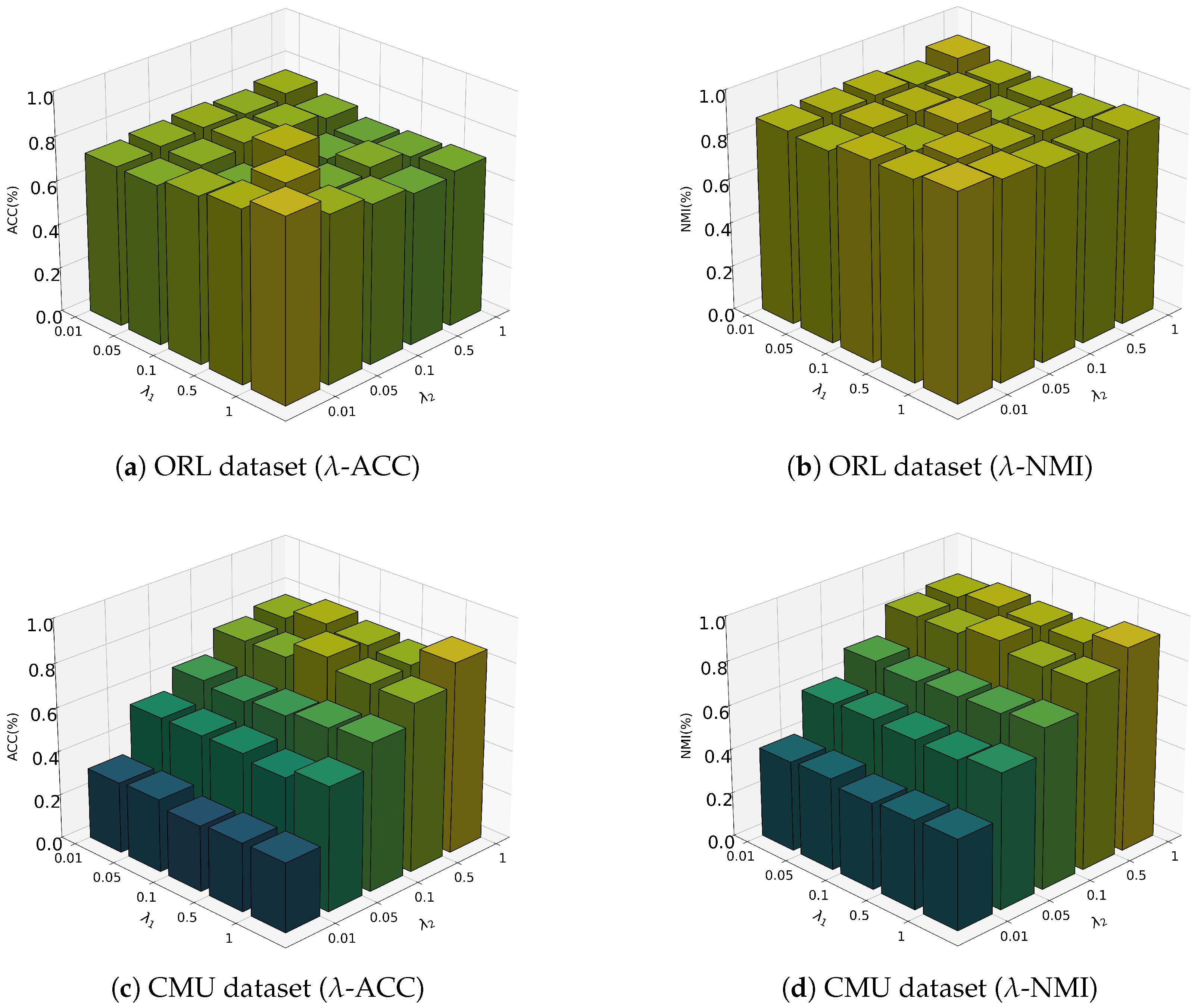
Sensitivity analysis of core regularization parameters ${\lambda }_1$ and ${\lambda }_2$. Fixing other parameters (consensus regularization term, matrix dimension reduction, and view weight temperature), we examine the performance variation of ${\lambda }_1$ and ${\lambda }_2$ over the range $\{0.01,0.05,0.1,0.5,1\}$. As shown in Figure 2, the key findings are as follows:

• Dataset differences: The model is more sensitive to parameters on the CMU dataset (due to larger view differences) while showing smaller variations on the ORL dataset (where view differences are smaller).
• Parameter impact: ${\lambda }_1$ has a significantly larger impact on performance than ${\lambda }_2$, indicating that the low-rankness of the latent representation matrix W is more critical than that of the projection matrix S.
• Optimal range: The best performance is achieved when ${\lambda }_1=1$ and ${\lambda }_2\in [0.01,1]$.

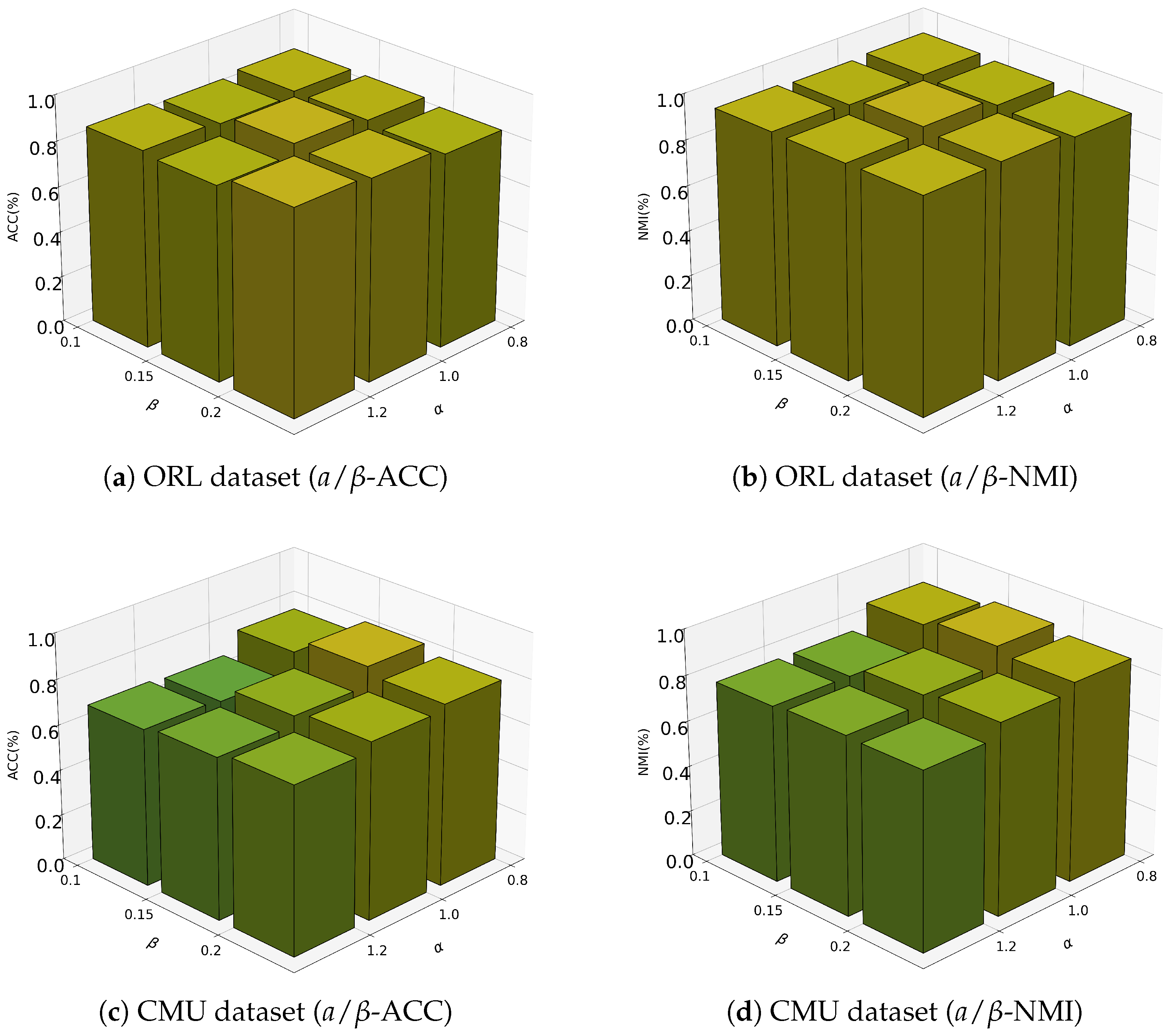
Sensitivity analysis of auxiliary parameters a and $\beta$. To explore the influence of dimension reduction and view weighting, we plot heatmaps of parameters a (controlling the strength of dimension reduction and the dimensionality m of the latent representation W and the projection matrix) and $\beta$ (controlling view weight allocation). The results are shown in Figure 3:

• Dimension reduction parameter a: Lower dimensions yield better performance. This parameter controls the size m of the latent representation matrix W and the projection matrix; a larger a leads to a larger m. When $a\in [0.1,0.2]$, ACC and NMI are highest, indicating that low-dimensional constraints effectively filter noise and focus on the consensus structure.
• View weight parameter $\beta$: This hyperparameter controls the distribution of view weights; a larger $\beta$ leads to more unbalanced weights. The optimal range is $\beta \in [0.8,1.2]$, where the model achieves stable and robust performance without requiring fine-grained tuning.

Sensitivity analysis of consensus regularization parameter ${\lambda }_3$. The parameter ${\lambda }_3$ controls the strength of learning the consensus representation matrix $W^{\ast }$. We evaluate its sensitivity across a range of values $\{0.01,0.05,0.1,0.5,1\}$. Experiments show that the value of ${\lambda }_3$ is closely related to the degree of view differences, as detailed below:

• Negative correlation between view differences and parameter value: When view differences are small (e.g., ORL dataset), a larger ${\lambda }_3$ (e.g., ${\lambda }_3\ge 0.5$) enhances consensus representation learning and improves clustering accuracy. Conversely, when view differences are large (e.g., CMU dataset), a smaller ${\lambda }_3$ (e.g., ${\lambda }_3\le 0.1$) suppresses overfitting to differences and maintains model stability.
• Robustness and adaptability: The model can achieve competitive performance on datasets with different view differences by adaptively adjusting ${\lambda }_3$, verifying the importance of this module in multi-view fusion.

Since ${\lambda }_3$ primarily affects internal model mechanisms rather than visualizable metrics, no corresponding figure is provided here; instead, the effectiveness of its value strategy is validated through experiments.

4.9. Convergence Analysis

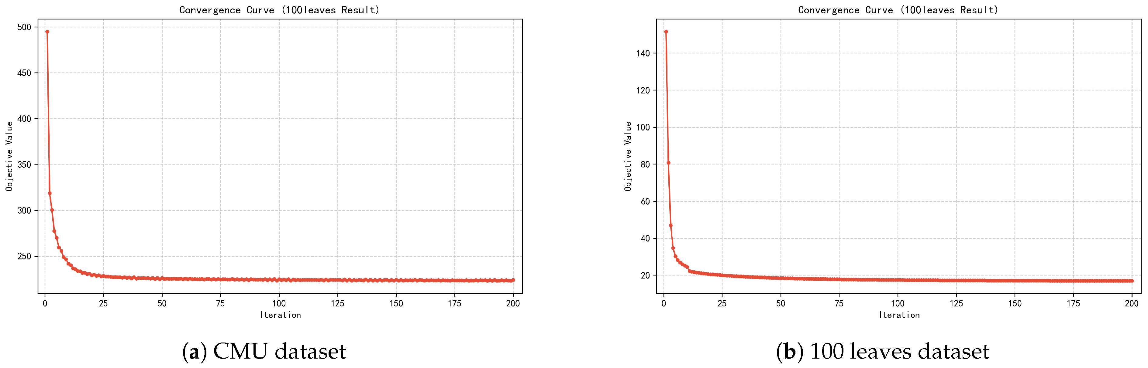
To verify the stability and efficiency of the proposed optimization algorithm, we conduct convergence analysis experiments on two benchmark datasets, CMU and 100 leaves. Figure 4a,b show the evolution of the objective function value with respect to the number of iterations on these two datasets.

From Figure 4a, it can be observed that on the CMU dataset, the objective function value decreases rapidly within the first 20 iterations; then, the decreasing rate gradually slows down and stabilizes after about 50 iterations. This phenomenon indicates that the algorithm can quickly capture the main structural features of the data in the early stage, refine them in subsequent iterations, and eventually converge within 200 iterations.

Similarly, Figure 4b shows the convergence behavior on the 100 leaves dataset. Despite the difference in datasets, the algorithm still exhibits excellent convergence performance: the objective function value drops sharply within the first 10 iterations, enters a plateau after about 20 iterations, and remains almost constant in later iterations. This further verifies that the proposed algorithm has fast convergence properties and can effectively optimize the objective function within a limited number of iterations.

Overall, the proposed algorithm converges within about 50 iterations on different datasets, which not only demonstrates the effectiveness of the optimization scheme but also indicates high computational efficiency for practical applications.

4.10. Visualization Analysis

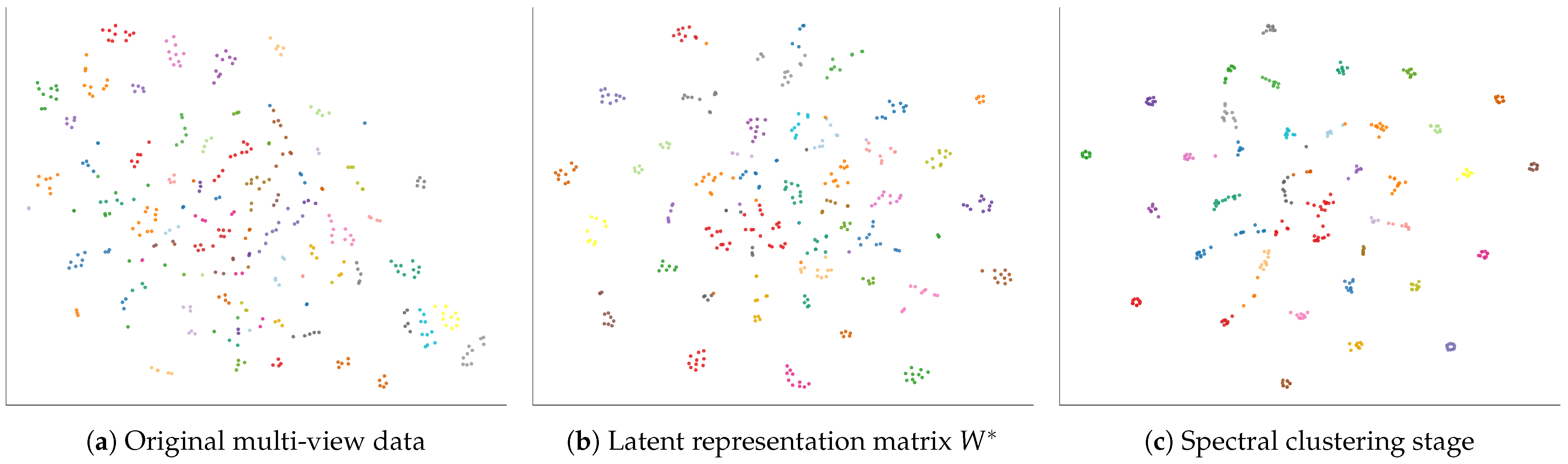
To intuitively evaluate the discriminative ability of the latent representations learned by our proposed method, we use t-SNE to map the high-dimensional features into a two-dimensional plane for visualization. Figure 5 shows on the ORL dataset: (a) the original multi-view data, (b) the latent representation matrix $W^{\ast }$ learned by our method, and (c) the sample distribution at the spectral clustering stage, where different colors represent different true class labels.

By comparing the three subfigures, we observe the following:

• Figure 5a Original data. The sample points are highly mixed in the two-dimensional space. Samples of the same class are scattered across different regions, and samples of different classes overlap considerably. This suggests that the original multi-view features contain substantial noise and redundant information, and they lack a clear structure suitable for direct clustering.
• Figure 5b Latent representation matrix $W^{\ast }$. Compared with the original data, after feature learning, samples of the same class begin to aggregate, showing a discernible clustering tendency. However, intra-class samples remain relatively loose, and the boundaries between multiple classes are not fully separated. This indicates that the latent representation matrix $W^{\ast }$ alone may not be sufficient to distinguish all classes clearly.
• Figure 5c Spectral clustering stage. After performing spectral clustering using $W^{\ast }$, a clearer cluster structure emerges. Intra-class compactness is improved: sample points of the same color are more tightly grouped, forming identifiable cluster centers. Inter-class separability is also enhanced: clusters of different colors appear more distinct with reduced overlap. This distribution pattern, characterized by higher intra-class cohesion and inter-class separation, is a desirable property for clustering representations.

The above visualization results suggest that the combination of matrix factorization and spectral clustering yields favorable clustering performance on the evaluated data. The regularization framework proposed in this paper captures high-order correlations in multi-view data and reduces noise interference, leading to a more discriminative consensus latent representation. This observation is consistent with the quantitative experimental results presented in previous sections, supporting the effectiveness of the proposed approach from both qualitative and quantitative perspectives.

4.11. Time Complexity Analysis

To comprehensively evaluate the computational efficiency of the proposed DTCMVSC method and its counterparts, we conduct a theoretical time complexity analysis.

Table 6. Time complexity comparison of multi-view clustering methods.

Method	Time Complexity (Dominant)
AFMC	$O\left(TVndr\right)$
MvSCGE	$O\left(TV{n}^3\right)$
TPCH	$O\left(V(m^{3}l+nml+n{m}^2+nllogn+ncl)\right)$
CSMSC	$O\left(MV{n}^3\right)$
MVC-WA	$O(n{m}^{2}d+n{m}^{3}V+n{m}^2{V}^2)$
AGLDR	$O\left(Tnmd\right)$
3AMVC	$O(Vnd{m}_{max}+n{m}_b^2)$
Ours	$O\left(TVnd(m+k)+TVn{m}^2+n^{2}m\right)$

summarizes the asymptotic complexity expressions of all compared algorithms under unified symbolic conventions. For clarity, the dominant terms are reported, where n denotes the number of samples, V the number of views, d the average feature dimensionality (or sum of dimensions depending on context), m the number of anchors (if applicable), k the reduced rank or intermediate dimension, c the number of clusters, r the length of binary hash codes, l the hash code length (for TPCH), and T the number of iterations. The expressions reveal the scalability bottlenecks of each method with respect to the sample size n.

For the proposed DTCMVSC method, the overall complexity comprises three additive components:

• Matrix factorization updates: $O\left(TVnd\right(m+k\left)\right)$, linear in n and dominated by matrix multiplications.
• Double tensor nuclear norm proximal operators: $O\left(TVn{m}^2\right)$, originating from slice-wise SVD in the Fourier domain.
• Spectral clustering stage: $O\left(n^{2}m\right)$, which is required for constructing the similarity matrix from the final consensus representation.

In typical settings, $m,k\ll \min (n,d)$ and V is small, rendering the iterative phase highly efficient. The quadratic term appears only once after convergence and can be mitigated via anchor-based approximations if necessary.

5. Conclusions

This paper proposed a dual-tensor constrained multi-view subspace clustering method (DTCMVSC) based on three-factor matrix factorization. By imposing tensor nuclear norm regularization on both the latent representation and projection matrices, the model captures high-order cross-view correlations while preserving view-specific characteristics. A consensus term with adaptive weights aligns representations across views, and spectral clustering on the resulting consensus matrix yields final labels. Experiments on six benchmarks demonstrate the effectiveness of the approach with particularly strong results on CMU and ORL.

Several directions merit further exploration. First, extending the linear factorization to deep or kernel-based formulations could better model nonlinear data relationships. Second, developing more efficient tensor approximations would improve scalability to very large datasets. Third, adapting the framework to incomplete multi-view scenarios would broaden its practical applicability. Finally, incorporating limited label information via semi-supervised learning may further enhance clustering accuracy in challenging cases.

References

1. Zhang, R.; Nie, F.; Li, X.; Wei, X. Feature selection with multi-view data: A survey. Inf. Fusion 2019, 50, 158–167. [Google Scholar] [CrossRef]
2. Yang, Y.; Wang, H. Multi-view clustering: A survey. Big Data Min. Anal. 2018, 1, 83–107. [Google Scholar] [CrossRef]
3. Xu, C.; Tao, D.; Xu, C. A survey on multi-view learning. arXiv 2013, arXiv:1304.5634. [Google Scholar] [CrossRef]
4. Gao, H.; Nie, F.; Li, X.; Huang, H. Multi-view subspace clustering. In Proceedings of the IEEE International Conference on Computer Vision (ICCV), Santiago, Chile, 7–13 December 2015; pp. 4238–4246. [Google Scholar]
5. Zhang, C.; Fu, H.; Hu, Q.; Cao, X.; Xie, Y.; Tao, D.; Xu, D. Generalized latent multi-view subspace clustering. IEEE Trans. Pattern Anal. Mach. Intell. 2018, 42, 86–99. [Google Scholar] [CrossRef]
6. Luo, S.; Zhang, C.; Zhang, W.; Cao, X. Consistent and specific multi-view subspace clustering. In Proceedings of the AAAI Conference on Artificial Intelligence, New Orleans, LA, USA, 2–7 February 2018; Association for the Advancement of Artificial Intelligence (AAAI): Washington, DC, USA, 2018; Volume 32. [Google Scholar]
7. Chen, Z.; Wu, X.-J.; Xu, T.; Kittler, J. Fast self-guided multi-view subspace clustering. IEEE Trans. Image Process. 2023, 32, 6514–6525. [Google Scholar] [CrossRef]
8. Li, Z.; Tang, C.; Zheng, X.; Liu, X.; Zhang, W.; Zhu, E. High-order correlation preserved incomplete multi-view subspace clustering. IEEE Trans. Image Process. 2022, 31, 2067–2080. [Google Scholar] [CrossRef]
9. Zheng, Q.; Zhu, J.; Li, Z.; Pang, S.; Wang, J.; Li, Y. Feature concatenation multi-view subspace clustering. Neurocomputing 2020, 379, 89–102. [Google Scholar] [CrossRef]
10. Sun, X.; Cheng, M.; Min, C.; Jing, L. Self-supervised deep multi-view subspace clustering. In Proceedings of the Asian Conference on Machine Learning (ACML), Nagoya, Japan, 17–19 November 2019; pp. 1001–1016. [Google Scholar]
11. Huang, S.; Wu, H.; Ren, Y.; Tsang, I.; Xu, Z.; Feng, W.; Lv, J. Multi-view subspace clustering on topological manifold. Adv. Neural Inf. Process. Syst. 2022, 35, 25883–25894. [Google Scholar]
12. Khan, A.; Maji, P. Multi-manifold optimization for multi-view subspace clustering. IEEE Trans. Neural Netw. Learn. Syst. 2021, 33, 3895–3907. [Google Scholar] [CrossRef]
13. Si, X.; Yin, Q.; Zhao, X.; Yao, L. Consistent and diverse multi-view subspace clustering with structure constraint. Pattern Recognit. 2022, 121, 108196. [Google Scholar] [CrossRef]
14. Wei, S.; Wang, J.; Yu, G.; Domeniconi, C.; Zhang, X. Multi-view multiple clusterings using deep matrix factorization. In Proceedings of the Proceedings of the AAAI Conference on Artificial Intelligence, New York, NY, USA, 7–12 February 2020; Volume 34, pp. 6348–6355. [Google Scholar]
15. Cao, X.; Zhang, C.; Fu, H.; Liu, S.; Zhang, H. Diversity-induced multi-view subspace clustering. In Proceedings of the IEEE Conference on Computer Vision and Pattern Recognition (CVPR), Boston, MA, USA, 7–12 June 2015; IEEE: New York, NY, USA, 2015; pp. 586–594. [Google Scholar]
16. Wang, Y.; Lin, X.; Wu, L.; Zhang, W.; Zhang, Q.; Huang, X. Robust subspace clustering for multi-view data by exploiting correlation consensus. IEEE Trans. Image Process. 2015, 24, 3939–3949. [Google Scholar] [CrossRef]
17. Yang, B.; Zhang, X.; Nie, F.; Wang, F.; Yu, W.; Wang, R. Fast multi-view clustering via nonnegative and orthogonal factorization. IEEE Trans. Image Process. 2020, 30, 2575–2586. [Google Scholar] [CrossRef]
18. Zhao, J.; Lu, G.-F. Clean affinity matrix learning with rank equality constraint for multi-view subspace clustering. Pattern Recognit. 2023, 134, 109118. [Google Scholar] [CrossRef]
19. Yang, Z.; Tan, Y.; Yang, T. Large-scale multi-view clustering via matrix factorization of consensus graph. Pattern Recognit. 2024, 155, 110716. [Google Scholar] [CrossRef]
20. Li, J.; Shen, X.; Li, C.; Li, Y. Elements discriminative non-negative matrix factorization for data clustering. Eng. Appl. Artif. Intell. 2025, 156, 111210. [Google Scholar] [CrossRef]
21. Zheng, X.; Tang, C.; Liu, X.; Zhu, E. Multi-view clustering via matrix factorization assisted k-means. Neurocomputing 2023, 534, 45–54. [Google Scholar] [CrossRef]
22. Wang, R.; Gao, Q.; Yang, M.; Wang, Q. Tensorized tri-factor decomposition for multi-view clustering. IEEE Trans. Circuits Syst. Video Technol. 2025, 35, 5355–5366. [Google Scholar] [CrossRef]
23. Zeng, Y.; Song, P.; Yang, B.; Wang, C.; Du, G.; Yu, Y.; Zheng, W. Hypergraph regularization-based anchor learning for multi-view clustering. Pattern Recognit. 2025, 172, 112465. [Google Scholar] [CrossRef]
24. Zhang, Y.; Lu, G.-F. Tensorized multi-dimensional multi-view clustering based on nonnegative matrix factorization. Neural Netw. 2025, 197, 108507. [Google Scholar] [CrossRef] [PubMed]
25. Zhang, X.; Leng, C.; Peng, J.; Cheng, I.; Basu, A. Orthogonal diversity nonnegative matrix factorization for multi-view clustering. Eng. Appl. Artif. Intell. 2025, 152, 110715. [Google Scholar] [CrossRef]
26. Liang, N.; Yang, Z.; Xiang, D.; Xu, J.; Zhou, G.; Xie, S. Localization graph generation based matrix factorization for incomplete multi-view clustering. IEEE Trans. Emerg. Top. Comput. 2026, 14, 196–209. [Google Scholar] [CrossRef]
27. Khalafaoui, Y.; Matei, B.; Lovisetto, M.; Grozavu, N. Deep matrix factorization with adaptive weights for multi-view clustering. Pattern Recognit. 2026, 170, 112027. [Google Scholar] [CrossRef]
28. Chen, M.-S.; Huang, L.; Wang, C.-D.; Huang, D.; Yu, P.S. Multiview subspace clustering with grouping effect. IEEE Trans. Cybern. 2020, 52, 7655–7668. [Google Scholar] [CrossRef] [PubMed]
29. Bian, J.; Xie, X.; Wang, C.-D.; Yang, L.; Lai, J.-H.; Nie, F. Angular reconstructive discrete embedding with fusion similarity for multi-view clustering. IEEE Trans. Knowl. Data Eng. 2025, 37, 45–59. [Google Scholar] [CrossRef]
30. Deng, P.; Zhou, X.; Xu, J.; Huang, W.; Wang, J.; Wang, D.; Li, T. Symmetric non-negative matrix factorization-based deep representation algorithm for multi-view clustering. Eng. Appl. Artif. Intell. 2025, 162, 112738. [Google Scholar] [CrossRef]
31. Cui, J.; Liufu, B.; Fu, Y.; Wang, M.; Lai, Z. Nonlinear multi-view clustering for non-negative matrix factorization. Neural Netw. 2025, 191, 107744. [Google Scholar] [CrossRef]
32. Wen, J.; Xu, G.; Tang, Z.; Wang, W.; Fei, L.; Xu, Y. Graph regularized and feature aware matrix factorization for robust incomplete multi-view clustering. IEEE Trans. Circuits Syst. Video Technol. 2023, 34, 3728–3741. [Google Scholar] [CrossRef]
33. Dong, Y.; Che, H.; Leung, M.-F.; Liu, C.; Yan, Z. Centric graph regularized log-norm sparse non-negative matrix factorization for multi-view clustering. Signal Process. 2024, 217, 109341. [Google Scholar] [CrossRef]
34. Wang, S.; Liu, X.; Zhu, X.; Zhang, P.; Zhang, Y.; Gao, F.; Zhu, E. Fast parameter-free multi-view subspace clustering with consensus anchor guidance. IEEE Trans. Image Process. 2021, 31, 556–568. [Google Scholar] [CrossRef]
35. Liu, S.-Y.; Wang, S.-W.; Tang, C.; Zhou, S.-H.; Wang, S.-Q.; Liu, X.-W. Multi-view clustering with weighted anchors. Acta Autom. Sin. 2024, 50, 1160–1170. [Google Scholar]
36. Chen, Z.; Zhu, M.; Li, H.; Xu, T. Anchor graph learning with double noise removal for multi-view clustering. Neural Netw. 2025, 191, 107779. [Google Scholar] [CrossRef]
37. Ma, H.; Wang, S.; Yu, S.; Liu, S.; Huang, J.-J.; Wu, H.; Liu, X.; Zhu, E. Automatic and aligned anchor learning strategy for multi-view clustering. In Proceedings of the 32nd ACM International Conference on Multimedia, Melbourne, Australia, 28 October–1 November 2024; Association for Computing Machinery: New York, NY, USA, 2024; pp. 5045–5054. [Google Scholar]
38. Yang, T.; Wang, C.-D.; Guo, J.; Li, X.; Chen, M.-S.; Dang, S.; Chen, H. Triplets-based large-scale multi-view spectral clustering. Inf. Fusion 2025, 121, 103134. [Google Scholar] [CrossRef]
39. Zhong, G.; Pun, C.-M. Self-taught multi-view spectral clustering. Pattern Recognit. 2023, 138, 109349. [Google Scholar] [CrossRef]
40. Yang, B.; Zhang, X.; Wu, J.; Nie, F.; Wang, F.; Chen, B. Scalable min-max multi-view spectral clustering. IEEE Trans. Knowl. Data Eng. 2025, 37, 2918–2931. [Google Scholar] [CrossRef]
41. Shi, L.; Ye, Y.; Cao, L.; Zhao, Y.; Chen, B. Tensor-based graph learning with consistency and specificity for multi-view clustering. IEEE Trans. Multimed. 2025, 28, 1562–1575. [Google Scholar] [CrossRef]
42. Zhang, J.; Zhang, X.; Yang, Y.; Li, J.; Ren, Z.; Tang, R.; Wang, D. Dual-tensor collaborative facilitation for multi-view clustering. Expert Syst. Appl. 2025, 298, 129883. [Google Scholar] [CrossRef]
43. Qian, L.; Chen, M.; Ma, X.; Zhang, C.; Zhang, J. Multi-view clustering based on adaptive tensor singular value shrinkage. Comput. Res. Dev. 2025, 62, 733–750. [Google Scholar]
44. Wang, Z.; Li, X.; Sun, Y.; Sun, Q.; Sun, Y.; Ling, H.; Dai, J.; Ren, Z. TPCH: Tensor-interacted projection and cooperative hashing for multi-view clustering. In Proceedings of the AAAI Conference on Artificial Intelligence, Philadelphia, PA, USA, 25 February–4 March 2025; Association for the Advancement of Artificial Intelligence: Washington, DC, USA, 2025; Volume 39, pp. 21420–21428. [Google Scholar]
45. Li, Q.; Yang, G.; Yun, Y.; Lei, Y.; You, J. Tensorized discrete multi-view spectral clustering. Electronics 2024, 13, 491. [Google Scholar] [CrossRef]
46. Long, Z.; Wang, Q.; Ren, Y.; Liu, Y.; Zhu, C. TLRLF4MVC: Tensor low-rank and low-frequency for scalable multi-view clustering. IEEE Trans. Pattern Anal. Mach. Intell. 2025, 47, 6900–6911. [Google Scholar] [CrossRef]
47. Shen, Q.; Xu, T.; Liang, Y.; Chen, Y.; He, Z. Robust tensor recovery for incomplete multi-view clustering. IEEE Trans. Multimed. 2023, 26, 3856–3870. [Google Scholar] [CrossRef]
48. Huang, S.; Fu, L.; Du, S.; Wu, Z.; Vasilakos, A.V.; Wang, S. Low-rank tensor learning with projection distance metric for multi-view clustering. Int. J. Mach. Learn. Cybern. 2025, 16, 25–41. [Google Scholar] [CrossRef]
49. Boyd, S.; Parikh, N.; Chu, E.; Peleato, B.; Eckstein, J. Distributed optimization and statistical learning via the alternating direction method of multipliers. Found. Trends Mach. Learn. 2011, 3, 1–122. [Google Scholar] [CrossRef]
Figure 1. Overview of the DTCMVSC Algorithm Framework. Tensor nuclear norm regularization is imposed on the entire tensor structure. Specifically, the tensor is transformed to the frequency domain via fast Fourier transform (FFT), and then t-SVD is applied to the frequency-domain tensor to obtain a low-dimensional representation. By minimizing the tensor nuclear norm (i.e., the sum of the singular values of the tensor t-SVD), we effectively enforce the low-rankness of the tensor, thereby obtaining the optimal low-rank representation for multi-view fusion. On this basis, an adaptive weighting mechanism is used to fuse information from different views into a consensus matrix W , which is then used to construct a similarity matrix, and finally spectral clustering yields the clustering results.
Applsci 16 04766 g001
Figure 2. Sensitivity analysis of core regularization parameters λ 1 and λ 2 . The model exhibits higher sensitivity on the CMU dataset (due to larger view differences), and λ 1 has a significantly larger impact on performance than λ 2 .
Applsci 16 04766 g002
Figure 3. Sensitivity analysis of auxiliary parameters a (dimension reduction) and β (view weight). Lower dimensions ( a [ 0.1 , 0.2 ] ) yield better performance, and performance is stable for β [ 0.1 , 1.0 ] .
Applsci 16 04766 g003
Figure 4. Convergence analysis curves of the algorithm.
Applsci 16 04766 g004
Figure 5. Visualization analysis using t-SNE on the ORL dataset. (a) Sample distribution of the original multi-view data, where classes are heavily mixed; (b) latent representation matrix W learned by our method, showing discernible clustering tendency; (c) low-dimensional representation obtained in the spectral clustering stage, exhibiting improved intra-class compactness and inter-class separability.
Applsci 16 04766 g005