A Novel Gene Expression Programming Algorithm for Forecasting Carbon Dioxide Emissions in G7 Countries

Abstract

The increase in the carbon dioxide (CO₂) emissions, nearly a quarter of those originating from the G7 countries, threatens not only the sustainability of the Earth but also the lives of future generations of humanity. Shedding light on future projections of the CO₂ emissions is vital in achieving the target of carbon neutrality, and machine learning-based algorithms are frequently applied to forecast the CO₂ emissions in the literature. However, the majority of these algorithms create model equations that are abstruse and irreproducible. In the current study, a novel gene expression programming (GEP) algorithm is proposed to produce genuine and easily understandable mathematical models for forecasting the CO₂ emissions of the G7 countries. The proposed algorithm is comprehensively compared with both the simple GEP and the previous studies in terms of several error metrics and computational time. Consequently, the obtained results unveiled that the proposed algorithm surpassed the simple GEP by the improvements of 26% in nMAE, 24% in nRMSE, and 27% in MAPE, respectively. Notably, the proposed algorithm maintains essentially the same computational efficiency as the simple GEP (a 0.2% difference in duration) despite its richer function set. In addition to those, the estimated model equations belonging to the year of 2035 were meticulously presented to guide the researchers in the field for the sake of applicability and reproducibility.

1. Introduction

Climate change is an inevitable global problem that needs to be overcome urgently [1]. The rapid development of the global economy and the improvement in living standards have led to an exponential increase in energy consumption and exposure to large amounts of greenhouse gas (GHG) emissions [2,3,4]. The most destructive effect of GHG emissions on society and the environment is global warming. The largest share of GHG emissions belongs to CO₂ emissions, with 76% [5], and increasing emissions in the atmosphere are the primary source of global warming [6,7]. The rising temperature of the Earth’s surface causes the melting of glaciers and rising sea levels. Such drastic climate changes are expected to have devastating consequences for crops, human health, ecological balance, and biodiversity in both the short and long term [8,9,10,11]. Global warming not only threatens the survival of the Earth but also endangers the sustainability of future generations of humankind [12,13,14,15]. Finally, Panmao Zhai, Co-Chair of Working Group I, stated in the [16] report, “Climate change is already affecting every region on Earth in various ways. The changes we experience will increase with additional warming”, thus emphasizing the unintended results of an increase in CO₂ emissions.

International agreements signed from past to present within the scope of combating global warming and climate change are as follows: the UN Framework Convention on Climate Change, the Kyoto Protocol, the Paris Agreement, the Europe 2020 strategy, the 2030 energy policy framework vision, and the European Green Deal [17,18]. As a result of these agreements, most countries set targets to slow down global warming. However, the global temperature continued to rise as emissions could not be reduced to the desired levels [19,20]. It is noteworthy here that although human beings are aware of the devastating problems caused by climate change, they cannot take preventive measures [21].

The group consisting of Canada, France, Germany, Italy, Japan, the United Kingdom, and the United States is called the G7 countries. These countries have a share of approximately 30% of the world’s primary energy consumption (PEC) and represent a quarter of total CO₂ emissions [22]. Also, the G7 countries constitute about 58% of the global wealth, and such a high rate of economic growth leads to a huge increase in the use of energy resources [23]. Unfortunately, most of the G7 countries depend on non-renewable or non-clean energy resources that contribute to CO₂ emissions to meet energy demands [24]. Hence, the G7 countries have a high potential to release large amounts of CO₂ emissions in the coming years. Similarly, it is predicted that the world’s energy needs will increase exponentially in the future, especially in countries with high economic growth rates [25]. This underscores the complexity of efforts to reduce CO₂ emissions.

It is known that many factors cause CO₂ emissions as well as the combustion of fossil fuels [26,27]. Based on this, as stated by [28], real-time CO₂ emission measurements are generally not feasible, and there is always a delay. Therefore, estimating CO₂ emissions will help policymakers effectively monitor emissions and adjust long-term policies. For the forecast of CO₂ emissions, reference [29] explained that it will provide a foundation for the development of blockchain technology, which is a hot topic today; references [30,31] pointed out that it is the prerequisite for effective prevention and control of CO₂ emissions. In summary, the importance of forecasting CO₂ emissions to achieve carbon neutrality, a vital threshold in the fight against climate change, has been emphasized once again.

Many studies have been carried out on the estimation of CO₂ emissions in the literature. In these studies, researchers have proposed various algorithms, theories, and mathematical models by examining different regions and historical periods.

Table 1. Literature survey on CO₂ emission forecasting studies, summarizing for each reference the employed model, historical sample period, forecast interval, geographical region, and key predictor variables.

Reference	Model	Time Interval	Region	Predictor
[32]	GM	2001–2009	Taiwan	CO2
		2010–2012
[33]	GM	1980–2007	Brazil	CO2, GDP, PEC
		2004–2013
[34]	NGBM	1980–2009	China	CO2, CI, EI, GDP, PEC
		2009–2020
[35]	Regression	1971–2010	Türkiye	TP, GDP, EC
	Models	2011–2025
[36]	GRPM	2004–2010	BRICS	CO2, EU, GDP, UP
		2015–2020
[37]	LSSVM	1978–2012	China	MI, RC
		2008–2012
[38]	NGM	1953–2013	China	CO2
		2014–2020
[39]	MSFLA–LSSVM	1990–2016	China	CO2, TP, GDPpc, UL, ECS, IS
		2018–2025		EI, TCC, CI, IMP, EXP
[8]	Improved	1980–2012	China,	CO2
	PSO–GPR	2013–2020	Japan, USA
[40]	GEP	2001–2015	South Korea	EXP, GRDP, IMP, TFA, TP
		2016–2030
[41]	MIDAS-	1957–2014	USA	CO2, GDP
	BPNN	2010–2014
[42]	GRNN-	1980–2015	Canada,	CO2, REC
	GWO	1980–2015	Iran, Italy
[43]	MLR	1971–2014	Iran	CI, FFEP, GDP, PEU, TP
	MPR	2015–2030
[44]	GM	1995–2016	Türkiye	CO2
		2017–2025
[45]	LSSVM	1978–2015	China	CO2, EP, GDP, IEE, IS, UL
		2016–2020
[46]	GM	2005–2018	China	CO2
		2018–2030
[29]	GA, LSO,	1965–2017	12 Countries	CO2
	LSSVM	2018–2025
[47]	CFNGM	2000–2018	BRICS	CO2
		2019–2025
[48]	ECGM	2009–2019	BRICS	CO2
		2020–2023
[49]	DOLS, FMOLS,	1978–2014	G6	CO2, FDI, GDP, Loans, SMV, Trade
	System-GMM	2005–2014
[50]	DGM	2014–2019	APEC	CO2
		2020–2023
[51]	ARIMA, AVGM,	1993–2018	China,	CO2
	Verhulst	2008–2018	Russia
[52]	NEGM	2014–2019	53 Countries	PEC
		2020–2022
[27]	GRPM	2000–2017	China	CO2
		2018–2022
[53]	CNN, CNN–LSTM,	1972–2019	Bangladesh	CO2, ELC, GDP
	DNN, LSTM	2020–2021
[54]	ARIMA	1980–2016	South	CO2
		2015–2027	Africa
[55]	ANN, DL,	1970–2016	Türkiye	ECT, GDP
	SVM	2016–2050		TP, VK
[56]	Regression	1980–2020	BRICS,	GDPpc, TP, UP
		2025–2045	MINT
[57]	GM	2011–2020	China	GDP, PEC,
		2021–2025		TP, UL
[58]	AR, ARMA,	1949–2021	Pakistan	CO2
	NPAR, NNA	2022–2030
[59]	UNGMC, GMC,	2008–2019 2020–2025	China	CO2, PEC,
	DGPM, SVR,			GDPpc,
	BPNN, ARIMA			TP, UL
[60]	AGMC	2011–2019	China	CO2
		2020–2025
Current study	Improved	1966–2023	G7	FFEC, GDPpc, HEC, NEC, REC
	GEP	2024–2035		PEC, TP

provides a comprehensive summary of the studies conducted to forecast CO₂ emissions in the past years.

As can be seen from Table 1, among the studied regions, China, one of the countries with the highest CO₂ emissions, has been the focus. The other regions focused on were Iran, Türkiye, the USA, and the BRICS countries. It is also observed that the most frequently preferred forecasting method by researchers is the GM approach and its variants. Finally, it is understood that the variables most frequently used in the development of forecasting models are GDP, GDPpc, TP, CO₂ emissions, energy consumption, urbanization, imports, and exports.

As evidenced by the comprehensive literature survey presented in Table 1, no prior study appears to have applied GEP—either simple or enhanced—to forecast the CO₂ emissions of all G7 countries collectively. The closest related work [49] focuses on G6 countries and relies on panel econometric methods (DOLS, FMOLS, System-GMM) rather than machine learning-based forecasting. In addition, GEP, which has recently become an increasingly popular estimation method, has been applied in many areas [61,62,63]. However, the use of the proposed GEP algorithm has not yet been evaluated to forecast CO₂ emissions. Most previous studies have used data sets recorded up to 2020. Therefore, the impact of the pandemic and the tensions between Russia and Ukraine on CO₂ emissions has not yet been evaluated. These deficiencies in the literature constitute a research gap. The main objective of the current study is to fill this gap by using the proposed GEP algorithm to forecast the CO₂ emissions of the G7 countries.

The innovative contributions of this study to the existing literature can be listed as follows:

(i) To the best of the authors’ knowledge, this is the first study to estimate the CO₂ emissions of all G7 countries. These countries have made significant progress towards becoming carbon neutral and, according to Net Zero scorecards calculated based on Net Zero Tracker data, all countries except Italy and the USA have enacted their targets (

Table 2. Net-zero scorecards for the G7 countries [64], reporting for each country the target year for achieving carbon neutrality, the legal status of the target (in law vs. in policy documents), the type of target (e.g., emissions reduction), and the interim milestones.

Countries	Target Status	First Interim Target	Type of Interim Target	Target Year
Canada	*	2030	✓	2050
France	*	2030	✓	2050
Germany	*	2030	✓	2045
Italy	•	2030	✓	2050
Japan	*	2030	✓	2050
UK	*	2030	✓	2050
USA	•	2030	✓	2050
* In law    • In policy document   ✓ Emissions reduction

). Therefore, the findings from the current study are expected to attract considerable attention in the field.

(ii) The proposed GEP algorithm is applied to forecast CO₂ emissions between 2024 and 2035 by using annual data for the 1966–2023 period for the G7 countries. In this context, this study is the first of its kind and reveals the estimation performance of the proposed GEP algorithm in the relevant field, which can produce genuine and easily understandable mathematical models, unlike the previously implemented methods.

(iii) As highlighted by [65], energy sources and economic factors play a key role in CO₂ emissions. In this regard, in addition to PEC, REC, NEC, HEC, and FFEC have been included as inputs, and the model has been enriched so that the proposed model can forecast CO₂ emissions more accurately. This study is unique in that almost all energy sources are included in the proposed model.

(iv) This paper provides several innovative findings that will be very useful for the G7 countries in achieving their carbon-neutral goals and will contribute to the more effective implementation of measures. This study will provide valuable references to policy makers in the development of climate change and energy policies.

The rest of this article is organized as follows: the data collection and its sources are introduced, the relationship between input and output variables is examined, the descriptive statistical calculations of the data set are given, and the proposed GEP algorithm is explained in detail in Section 2. Statistical metrics and their formula used to evaluate the forecast performance are presented in Section 3. The empirical results obtained using the proposed GEP and simple GEP algorithms and their discussion are also presented in Section 3. Finally, the conclusions of this study are summarized and some recommendations are given for decision makers in Section 4.

2. Materials and Methods

2.1. Data Set Description

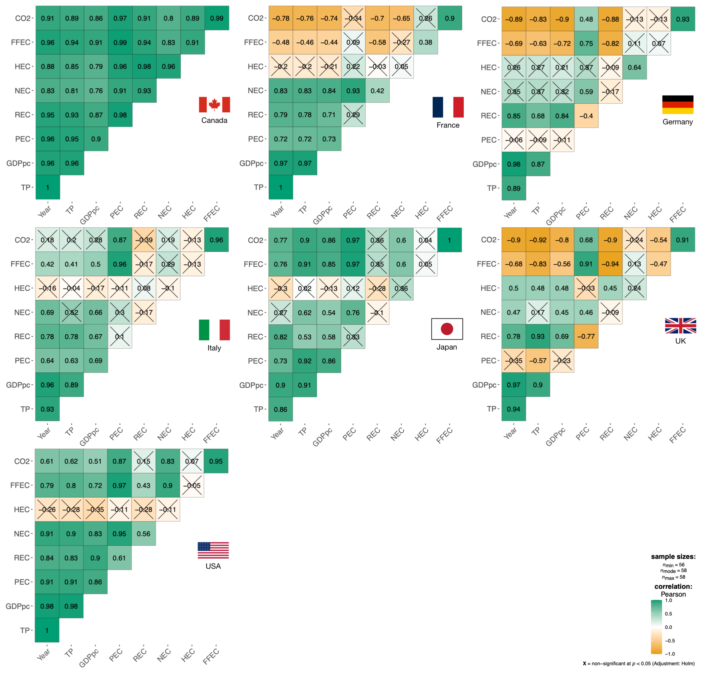
In the current study, the data set covers annual observations for each country in the G7 (Canada, France, Germany, Italy, Japan, the United Kingdom, and the United States) from 1966 to 2023, based on data availability. CO₂ emissions (CO₂, in million tons) are used as the dependent variable, while total population (TP), GDP per capita (GDPpc), primary energy consumption (PEC), renewable energy consumption (REC), nuclear energy consumption (NEC), hydroelectric energy consumption (HEC), and fossil-fuel energy consumption (FFEC) serve as explanatory variables. The definitions, units, and sources of these variables are summarized in

Table 3. Definition, units, and data sources for the variables used in the empirical analysis.

Variable	Units	Sources
CO2	Million tons	[66]
TP	Million persons	[22]
GDPpc	Current US$ (103)	[22]
PEC	Exajoules	[66]
REC	Exajoules	[66]
NEC	Exajoules	[66]
HEC	Exajoules	[66]
FFEC	Exajoules	[66]

, where data on CO₂, PEC, REC, NEC, HEC, and FFEC are obtained from the BP Statistical Review of World Energy [66], and TP and GDPpc are taken from the World Development Indicators [22]. Descriptive statistics for all variables and countries are reported in

Table 4. Descriptive statistics for CO₂ emissions and all explanatory variables in the G7 countries over the period 1966–2023.

Variables	Statistics	C	F	G	I	J	UK	USA
CO2	Min	271.7	252.9	571.9	222.7	503.8	320.9	3639.8
	Max	575.0	524.2	1116.4	470.2	1308.8	728.7	5885.0
	Median	464.5	379.9	894.7	377.7	1100.0	573.6	4975.8
	Mean	467.4	384.0	901.0	373.5	1070.6	561.1	4964.8
	SD	81.4	65.3	140.1	53.9	188.3	100.3	539.4
	SK	−0.5	0.4	−0.4	−0.5	−0.9	−0.8	−0.2
	KU	−0.7	0.0	−0.7	0.3	0.8	0.3	−0.3
TP	Min	20.0	49.8	76.6	52.5	98.9	54.6	196.6
	Max	40.1	68.2	84.5	60.8	128.1	68.4	334.9
	Median	29.2	59.4	80.6	56.8	125.0	57.9	264.7
	Mean	29.2	59.6	80.4	57.1	120.9	59.5	266.1
	SD	5.5	5.4	2.0	2.1	8.5	4.0	43.8
	SK	0.1	0.0	−0.1	0.0	−1.3	0.9	0.0
	KU	−1.1	−1.2	−0.2	−1.4	0.5	−0.5	−1.4
GDPpc	Min	3.1	2.2	1.9	1.5	1.1	2.0	4.1
	Max	55.5	45.5	52.7	40.9	49.1	50.4	81.7
	Median	21.2	23.0	25.4	20.7	33.3	21.8	28.2
	Mean	25.4	23.2	25.0	19.9	25.8	23.8	31.8
	SD	16.8	14.5	16.4	13.0	15.6	16.7	21.3
	SK	0.4	0.1	0.1	0.0	−0.4	0.1	0.5
	KU	−1.3	−1.4	−1.4	−1.5	−1.5	−1.6	−0.8
PEC	Min	5.3	5.0	10.7	3.6	7.5	7.0	54.9
	Max	14.7	11.5	15.8	7.9	22.9	9.8	97.4
	Median	12.0	9.7	14.3	6.5	18.7	8.9	86.7
	Mean	11.4	9.3	14.0	6.4	18.0	8.8	83.1
	SD	2.7	1.7	1.1	0.9	3.8	0.7	11.9
	SK	−0.6	−0.7	−1.2	−0.8	−0.8	−0.9	−0.6
	KU	−0.7	−0.1	1.4	1.1	0.4	0.5	−0.8
REC	Min	1.4	0.5	0.2	0.4	0.7	0.0	2.3
	Max	4.4	1.5	2.8	1.3	2.2	1.4	11.0
	Median	3.6	0.7	0.3	0.5	1.1	0.1	3.9
	Mean	3.3	0.8	0.8	0.6	1.1	0.3	4.7
	SD	0.9	0.2	0.8	0.3	0.3	0.4	2.2
	SK	−0.8	1.2	1.3	1.3	1.6	1.8	1.5
	KU	−0.5	1.1	0.2	−0.1	2.2	1.7	1.4
NEC	Min	0.0	0.0	0.0	0.0	0.0	0.2	0.1
	Max	1.1	4.5	1.7	0.1	3.3	1.0	8.3
	Median	0.8	3.4	0.9	0.0	1.1	0.6	6.8
	Mean	0.6	2.7	1.0	0.0	1.4	0.6	5.4
	SD	0.3	1.7	0.6	0.0	1.2	0.2	2.9
	SK	−0.9	−0.6	−0.2	1.5	0.3	0.2	−0.7
	KU	−0.8	−1.3	−1.4	1.4	−1.5	−1.0	−1.1
HEC	Min	1.4	0.4	0.1	0.3	0.7	0.0	2.1
	Max	3.8	0.8	0.3	0.6	1.0	0.1	3.8
	Median	3.5	0.6	0.2	0.4	0.8	0.1	2.8
	Mean	3.1	0.6	0.2	0.4	0.8	0.0	2.8
	SD	0.7	0.1	0.0	0.1	0.1	0.0	0.4
	SK	−1.1	0.2	0.3	−0.5	0.1	−0.4	0.4
	KU	−0.1	−0.8	1.3	1.7	−1.0	0.3	−0.2
FFEC	Min	3.9	4.2	8.6	3.1	6.6	5.2	52.5
	Max	9.6	7.3	15.0	7.4	18.9	9.3	84.9
	Median	7.4	5.9	12.5	5.6	15.8	8.3	74.5
	Mean	7.5	5.8	12.2	5.8	15.4	7.9	73.0
	SD	1.6	0.7	1.4	1.0	2.9	1.0	8.0
	SK	−0.4	−0.2	−0.4	−0.5	−1.1	−1.5	−0.5
	KU	−0.9	−0.1	−0.3	0.4	1.1	1.4	−0.4

, and the correlation structure is visualized in Figure 1.

Here, the USA has the highest mean value for all parameters except HEC. Canada is the country with the highest HEC value. Italy has the lowest CO₂, GDPpc, PEC, NEC, and FFEC values. The lowest values for TP, REC, and HEC were recorded in Canada, France, and the United Kingdom, respectively. For a data set to be normally distributed, its mean values should be greater than the SD values and the skewness and kurtosis values should be in the range of [−1,+1] and [−2,+2], respectively [18,67]. According to the results of the descriptive statistics, it is understood that the data set meets the normal distribution criteria for all parameters, except for a few exceptions.

The correlation chart describing the relationship between all variables is illustrated in Figure 1. The Pearson correlation coefficients indicate that there is a high degree of correlation between the independent variables and the dependent variable for the G7 countries in general. Moreover, several energy-related input variables (FFEC, PEC, REC, NEC, and HEC) are themselves highly correlated, reflecting the physical and statistical interdependencies among different components of energy consumption. As a result, it is understood that the data, with some exceptions, show a significant relationship and meet one of the basic assumptions for forecasting [68]. Since the primary aim of this study is forecasting rather than causal inference, these correlations are naturally accommodated within the symbolic regression framework of GEP, which searches over non-linear expressions and is typically less affected by multicollinearity issues than classical linear regression models [69].

Figure 1. Pearson correlation matrix of all variables used in the study for the G7 countries over the period 1966–2023 [70]. The figure displays the pairwise correlations between CO₂ emissions (CO₂) and the explanatory variables (total population (TP), GDP per capita (GDPpc), primary energy consumption (PEC), renewable (REC), nuclear (NEC), hydroelectric (HEC), and fossil-fuel energy consumption (FFEC)). Strong positive correlations are observed between CO₂ and energy-related variables, while the energy components themselves are also highly inter-correlated, reflecting their physical and statistical interdependencies.

Figure 1. Pearson correlation matrix of all variables used in the study for the G7 countries over the period 1966–2023 [70]. The figure displays the pairwise correlations between CO₂ emissions (CO₂) and the explanatory variables (total population (TP), GDP per capita (GDPpc), primary energy consumption (PEC), renewable (REC), nuclear (NEC), hydroelectric (HEC), and fossil-fuel energy consumption (FFEC)). Strong positive correlations are observed between CO₂ and energy-related variables, while the energy components themselves are also highly inter-correlated, reflecting their physical and statistical interdependencies.

It should also be noted that the dominant variable selected by GEP for each country (e.g., FFEC for Canada and France, REC for Germany) should be interpreted as an informative predictor under multicollinearity, not as a unique causal driver. Different, yet closely related, energy indicators may act as effective proxies for the underlying energy–emissions relationship in different national contexts, and caution is warranted when drawing causal inferences from these country-specific equations.

2.2. Methodological Framework

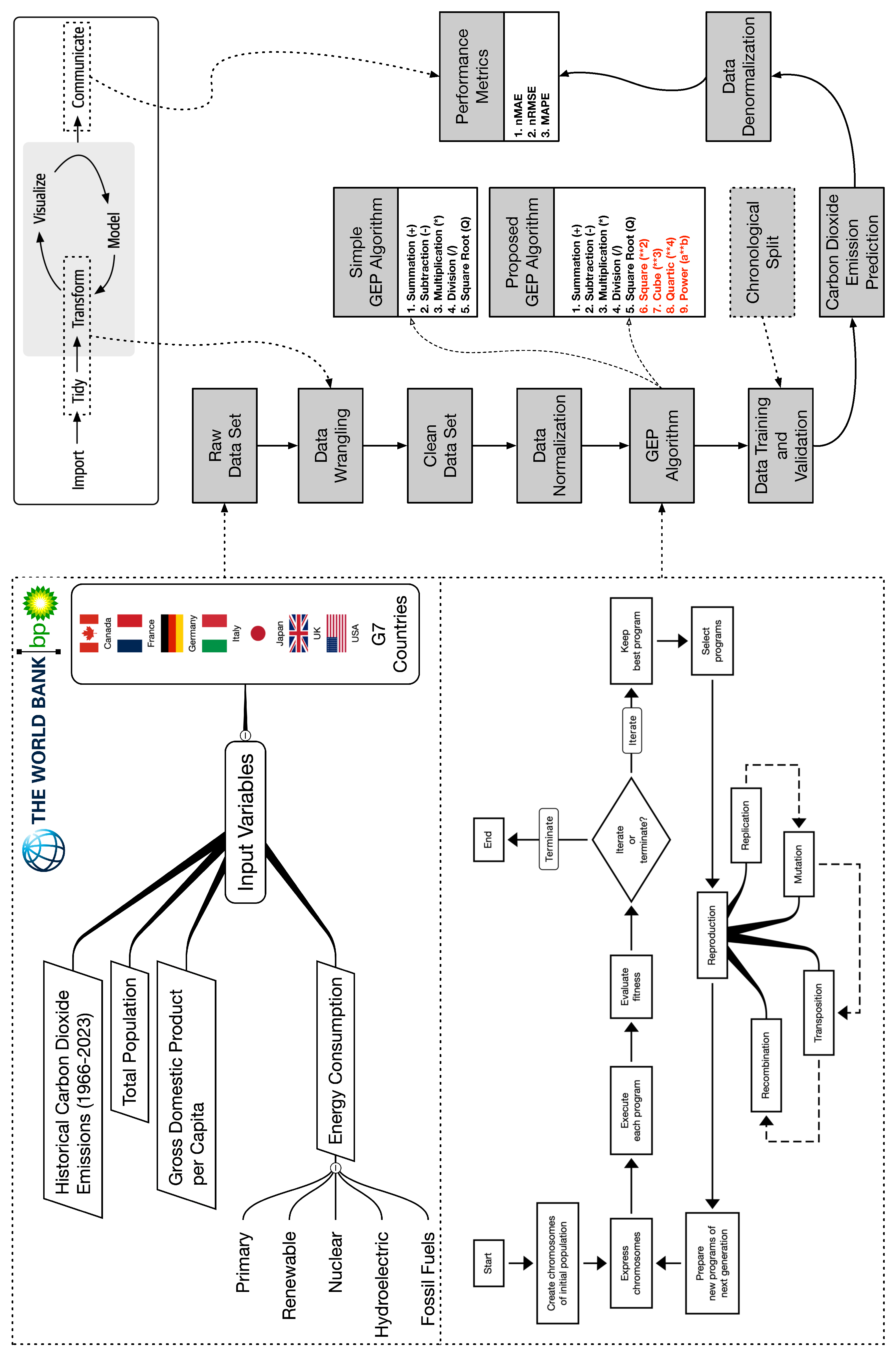
This study uses the proposed GEP model to estimate the CO₂ emissions of the G7 countries. Figure 2 shows the methodological framework of this study and consists of the following steps: (i) creating the data set; (ii) developing a novel GEP model; and (iii) forecasting CO₂ emissions in 2024–2035.

In this study, CO₂ emission forecasting is formulated as a supervised learning problem with a univariate output and multiple explanatory variables. For each country and year t, we define the vector of contemporaneous inputs as

$${\mathbf{x}}_t=\left(x_t^{\mathrm{CO}2},x_t^{\mathrm{TP}},x_t^{\mathrm{GDPpc}},x_t^{\mathrm{PEC}},x_t^{\mathrm{REC}},x_t^{\mathrm{NEC}},x_t^{\mathrm{HEC}},x_t^{\mathrm{FFEC}}\right),$$

where $x_t^{\mathrm{CO}2}$ denotes the observed CO₂ emissions at time t (used as a historical input), and the remaining components correspond to total population (TP), GDP per capita (GDPpc), primary energy consumption (PEC), renewable energy consumption (REC), nuclear energy consumption (NEC), hydroelectric energy consumption (HEC), and fossil-fuel energy consumption (FFEC), respectively. For each forecast horizon h ($h=1,\dots ,12$), the GEP model uses a feature vector

$${\mathbf{z}}_t=\left({\mathbf{x}}_t,{\mathbf{x}}_{t-1},\dots ,{\mathbf{x}}_{t-L}\right),$$

constructed from the contemporaneous and lagged inputs up to a maximum lag L and aims to learn a mapping $f_h(·)$ such that

$${\widehat{y}}_{t+h}=f_h\left({\mathbf{z}}_t\right),$$

where $y_{t+h}$ denotes the CO₂ emissions to be forecast h steps ahead.

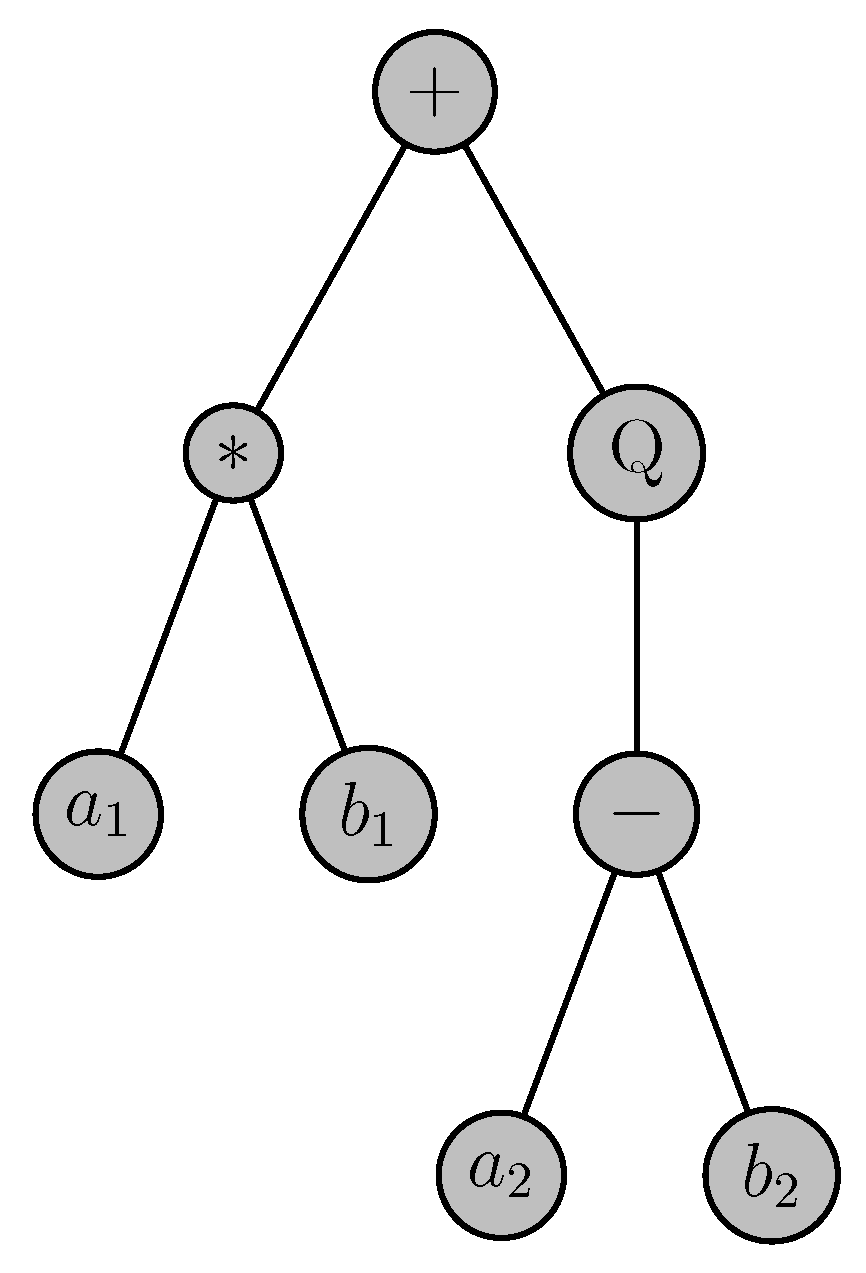
The GEP algorithm fundamentally resembles the genetic algorithm and genetic programming; however, the individuals are represented as linear strings of a fixed length that can then be described as nonlinear entities of different sizes and shapes such as expression trees in the GEP algorithm [71]. The GEP algorithm possesses the following basic elements: (i) function set, (ii) terminal set, (iii) fitness function, (iv) control parameters, and (v) termination condition [72]. A visualization belonging to a plain expression tree is demonstrated in Figure 3, and the character string of the expression tree is given in

Table 5. Character string representation of the expression tree illustrated in Figure 3.

Gene Character	0	1	2	3	4	5	6	7
Node representation	+	*	Q	$a_1$	$b_1$	–	$a_2$	$b_2$

[73].

The expression tree indicated in Figure 3 reflects the below equation:

$$y=a_1{b}_1+\sqrt{a_2-b_2}$$

The flowchart of the GEP algorithm is embedded in Figure 2. In brief, the operation initializes with random creation of chromosomes to yield the initial population. Subsequently, the expression of chromosomes and assessment of each individual’s fitness are fulfilled progressively. Later, the choices of individuals are conducted according to fitness for reproduction with alteration. The operation is reiterated for a preordained number of generations or before a final remedy [72].

Thanks to several advantages such as overcoming the limitations of the genetic algorithm and programming, being versatile, and being straightforward to interpret with its branched configuration, the GEP algorithm is selected to simply generate genuine mathematical models between explanatory variables and target variables in this study [73]. Despite its advantages, GEP is sensitive to the choice of hyperparameters (such as population size, head length, and mutation rates) and requires careful control of model complexity to avoid overfitting, particularly when the function set is extended with higher-degree operators.

Among the implementations of the GEP algorithm in the current literature, symbolic regression is an extensively chosen technique to acquire a mathematical relationship for a targeted output from explanatory variables of a given data set. The explanatory variables and outputs can be described as

$$\{x_{i,1},x_{i,2},\dots ,x_{i,n},y_{i,1},y_{i,2},\dots ,y_{i,m}\}$$

where n states the number of explanatory variables, m accounts for the number of outputs, and $x_{i,j}$ and $y_{i,j}$ are the jth input and output of the ith sample. Both mean squared error (MSE) and root mean squared error are often utilized for the accuracy of fitting. The symbolic regression seeks the optimal ${\mathrm{\Gamma }}^{*}$ which reduces the error to a minimum value for the data set

$${\mathrm{\Gamma }}^{*}={\arg }_{\mathrm{\Gamma }}\min f\left(\mathrm{\Gamma }\right)$$

where $\mathrm{\Gamma }$ is the formula’s quality parameter and $f\left(\mathrm{\Gamma }\right)$ results in the fitting error of $\mathrm{\Gamma }$ [72].

2.3. Proposed Algorithm

In the scope of this study, the simple GEP algorithm uses the standard allowed functions including summation (+), subtraction (−), multiplication (∗), division (/), and square root (Q) for all computations. Moreover, the proposed GEP algorithm employs both the standard functions and additional functions, namely square ($a^2$), cube ($a^3$), quartic ($a^4$), and power ($a^b$) functions wherein a and b may be stated as explanatory variables of the data set, as elaborated in Figure 2. Model building parameters for both the simple and proposed GEP algorithms are canonically utilized as follows:

• The magnitude of initial population: 50
• The count of utmost attempts for primary population: 10,000
• The quantity of genes per chromosome: 4
• The head length of gene: 8
• The quantity of utmost creations: 2000
• The quantity of creations without enhancement: 1000
• The termination value of the top chromosome’s fitness score: 1
• The fitness function: MSE
• The rates of evolution parameter:

  –

  Mutation: 44‰

  –

  Gene, inversion, and transposition: 10%

  –

  One-point and two-point recombination: 30%

• The linking function for all genes: Summation (+)
• Features of random constants:

  –

  Type of constants: Real (Floating point)

  –

  Random real constants per gene: 10

  –

  Least constant value: −10

  –

  Utmost constant value: 10

  –

  Mutation rate: 1%

2.4. Data Preprocessing and Partitioning

Min–max normalization eliminates the units of different data types in a data set, reduces the elapsed time for scientific computations, decreases memory usage, and allows a variety of features to be compared on a common scale [74]. Thus, values belonging to each cell of each data column representing a feature of the data set utilized in this study were normalized by a scaling operation among 0 and 1 [75]. To prevent data leakage, the minimum and maximum values required for min–max normalization were computed exclusively on the training set and subsequently applied to both the training and test sets.

For model testing and validation, the data set was divided into training and test sets in strictly chronological order, with the earlier 80% of observations (approximately 1966–2010) assigned to the training set and the most recent 20% (approximately 2011–2023) reserved as the test set. For each forecast horizon h ($h=1,2,\dots ,12$), a separate GEP model was trained using input variables lagged by h steps, ensuring that only historically available information was used during both training and prediction. This direct multi-step forecasting strategy effectively eliminates any possibility of look-ahead bias across all forecast horizons.

3. Results and Discussion

All computing tasks in the scope of this study were conducted on a Macintosh personal computer with an operating system version of 14.6.1, a central processing unit of 3.6 GHz (Intel Core i9 with 8 cores), and a random access memory size of 100 GB. The analyses were performed in the R (version 4.6.0) environment using RStudio (version 2026.01.1+403) as the integrated development environment, owing to its functionality and popularity in data science. The GEP models (both the simple GEP and the proposed GEP) were implemented with the gepR package [76], while model training and resampling procedures were managed using the caret package [77]. Data visualization and diagnostic plots, including the correlation charts, were produced with the ggplot2 and ggstatsplot packages [70,78].

As described in Section 2.4, all variables were min–max normalized and the data were split chronologically into training and test sets before model estimation.

To benchmark the obtained results pertaining to different countries in a likewise manner, normalized mean absolute error (nMAE), normalized root mean square error (nRMSE), and mean absolute percentage error (MAPE) metrics were chosen and used for the performance evaluation of all models in this study. The formulae of the aforementioned error metrics are demonstrated below:

$$nMAE(\%)={\displaystyle \frac{1}{n}}{\displaystyle \frac{{\sum }_{i=1}^n|y_i-{\widehat{y}}_i|}{\overline{y}}}\times 100$$

$$nRMSE(\%)={\displaystyle \frac{\sqrt{\frac{1}{n}{\sum }_{i=1}^n{(y_i-{\widehat{y}}_i)}^2}}{\overline{y}}}\times 100$$

$$MAPE(\%)={\displaystyle \frac{1}{n}}{\displaystyle \sum _{i=1}^n}{\displaystyle \frac{|y_i-{\widehat{y}}_i|}{|y_i|}}\times 100$$

where $y_i$ and ${\widehat{y}}_i$ denote the actual and forecasted values, respectively; $\overline{y}$ is the mean of the actual values and n is the number of observations [79,80,81,82]. The normalized metrics (nMAE and nRMSE) were selected to enable direct comparison across G7 countries whose CO₂ emissions differ substantially in magnitude (e.g., Italy ∼300 Mt vs. the USA ∼4600 Mt). MAPE is additionally reported because it is scale-independent and widely adopted in the CO₂ forecasting literature [42,55,83], facilitating comparisons with prior work.

In the performance tables for the G7 countries (

Table 6. h-step-ahead forecast performance of the simple GEP and proposed GEP models for Canada on the chronological test set (approximately 2011–2023).

Years	Simple GEP				Proposed GEP
	nMAE	nRMSE	MAPE	Duration	nMAE	nRMSE	MAPE	Duration
	(%)	(%)	(%)	(s)	(%)	(%)	(%)	(s)
2024	2.39	2.73	2.50	2.42	2.26	2.75	2.33	2.22
2025	3.02	3.68	3.41	3.12	2.18	2.73	2.26	3.77
2026	4.31	4.66	4.56	2.94	2.33	2.71	2.41	4.02
2027	2.89	4.08	3.09	3.13	2.00	2.96	2.37	3.48
2028	1.52	2.22	1.49	3.12	1.48	2.29	1.44	4.21
2029	2.24	2.81	2.16	3.83	1.68	2.34	1.56	3.40
2030	1.98	2.66	2.06	3.26	1.89	2.54	1.86	2.44
2031	1.81	2.24	1.83	3.03	1.46	1.80	1.45	2.79
2032	1.55	1.78	1.60	3.12	1.50	1.98	1.61	2.82
2033	3.00	3.44	3.03	4.91	1.56	2.31	1.51	6.28
2034	2.94	3.36	2.96	4.05	2.11	2.79	2.16	4.14
2035	2.40	2.92	2.36	4.28	2.36	2.88	2.33	5.50
Average	2.51	3.06	2.61	3.36	1.86	2.47	1.91	3.60
Improvement (%)					26.0	19.2	26.9	−7.2

,

Table 7. h-step-ahead forecast performance of the simple GEP and proposed GEP models for France on the chronological test set (approximately 2011–2023).

Years	Simple GEP				Proposed GEP
	nMAE	nRMSE	MAPE	Duration	nMAE	nRMSE	MAPE	Duration
	(%)	(%)	(%)	(s)	(%)	(%)	(%)	(s)
2024	5.39	7.04	6.04	1.66	4.69	6.06	5.23	1.76
2025	1.57	2.46	1.84	2.52	1.24	1.68	1.37	3.01
2026	1.98	3.43	2.14	4.02	2.27	2.90	2.43	2.85
2027	6.10	7.36	6.36	4.11	1.94	2.23	2.12	2.83
2028	1.25	1.44	1.35	2.43	1.20	1.47	1.30	2.12
2029	1.34	1.78	1.47	3.15	1.51	1.94	1.47	2.39
2030	2.79	3.38	3.03	2.80	1.44	1.79	1.42	2.59
2031	1.23	1.45	1.37	2.84	1.31	2.10	1.30	2.82
2032	1.19	1.36	1.24	2.93	0.90	1.17	1.02	2.78
2033	1.17	1.38	1.25	3.86	1.05	1.32	1.21	4.49
2034	1.53	1.96	1.51	5.02	1.40	1.79	1.34	5.46
2035	1.29	1.62	1.44	5.18	1.27	2.24	1.60	3.18
Average	2.24	2.89	2.42	3.38	1.69	2.22	1.82	3.02
Improvement (%)					24.5	23.0	24.9	10.5

,

Table 8. h-step-ahead forecast performance of the simple GEP and proposed GEP models for Germany on the chronological test set (approximately 2011–2023).

Years	Simple GEP				Proposed GEP
	nMAE	nRMSE	MAPE	Duration	nMAE	nRMSE	MAPE	Duration
	(%)	(%)	(%)	(s)	(%)	(%)	(%)	(s)
2024	2.93	3.36	3.08	2.46	2.65	3.02	2.67	2.16
2025	7.48	9.87	7.55	3.04	6.66	8.74	6.91	2.87
2026	4.46	5.20	4.41	3.60	3.98	4.80	3.93	3.00
2027	2.96	4.47	2.73	2.82	2.50	3.41	2.40	2.65
2028	6.21	6.93	6.42	2.56	3.51	5.09	3.25	2.96
2029	2.33	3.19	2.47	2.40	2.11	2.81	2.21	2.52
2030	4.21	4.50	4.28	2.58	4.01	5.04	3.83	3.40
2031	1.90	2.47	1.85	2.51	1.72	2.47	1.55	3.02
2032	2.68	3.82	2.57	2.82	2.13	3.39	1.95	3.12
2033	4.95	5.56	5.21	4.77	3.58	3.86	3.63	4.74
2034	1.61	1.90	1.55	4.96	1.80	2.64	1.71	7.22
2035	2.47	3.17	2.27	5.43	2.23	3.16	2.10	5.29
Average	3.68	4.54	3.70	3.33	3.07	4.04	3.01	3.58
Improvement (%)					16.5	11.0	18.6	−7.5

,

Table 9. h-step-ahead forecast performance of the simple GEP and proposed GEP models for Italy on the chronological test set (approximately 2011–2023).

Years	Simple GEP				Proposed GEP
	nMAE	nRMSE	MAPE	Duration	nMAE	nRMSE	MAPE	Duration
	(%)	(%)	(%)	(s)	(%)	(%)	(%)	(s)
2024	2.63	3.26	2.91	2.30	1.76	1.92	1.87	1.97
2025	2.27	4.05	2.81	4.35	2.60	3.17	2.62	2.68
2026	3.00	3.80	3.33	2.17	2.09	3.50	2.53	3.80
2027	2.68	3.35	2.84	2.99	2.32	2.74	2.40	2.76
2028	2.00	2.44	2.13	3.08	1.94	2.57	2.11	2.75
2029	1.72	2.52	1.91	3.39	1.68	2.01	1.75	2.67
2030	2.35	2.94	2.52	3.16	1.76	2.61	2.03	3.12
2031	2.22	2.72	2.43	2.97	2.16	3.15	2.36	2.86
2032	3.70	4.49	4.00	3.06	2.77	3.57	2.95	3.14
2033	2.52	3.10	2.67	3.37	2.23	2.64	2.27	4.38
2034	2.67	3.25	2.94	5.10	1.78	2.24	1.91	3.70
2035	2.18	2.47	2.34	3.96	1.77	2.63	2.04	4.44
Average	2.50	3.20	2.74	3.33	2.07	2.73	2.24	3.19
Improvement (%)					17.0	14.6	18.2	4.1

,

Table 10. h-step-ahead forecast performance of the simple GEP and proposed GEP models for Japan on the chronological test set (approximately 2011–2023).

Years	Simple GEP				Proposed GEP
	nMAE	nRMSE	MAPE	Duration	nMAE	nRMSE	MAPE	Duration
	(%)	(%)	(%)	(s)	(%)	(%)	(%)	(s)
2024	2.62	3.38	3.03	3.37	2.85	4.04	2.86	2.24
2025	7.78	9.53	8.98	3.32	4.42	7.31	6.19	4.21
2026	11.81	14.40	13.86	2.67	1.48	1.80	1.79	2.86
2027	3.12	3.62	3.08	2.97	0.53	0.62	0.56	3.58
2028	0.56	0.63	0.59	2.85	0.49	0.62	0.54	3.50
2029	0.38	0.42	0.39	2.88	0.92	1.07	1.06	3.27
2030	2.51	2.82	2.45	2.45	2.26	2.46	2.23	2.94
2031	0.68	0.92	7.56	3.67	0.64	0.90	0.70	2.25
2032	0.60	0.84	0.67	2.57	0.58	0.75	0.59	2.60
2033	0.54	0.65	0.57	7.34	0.51	0.64	0.55	5.84
2034	0.51	0.58	0.55	6.26	0.34	0.38	0.35	4.61
2035	0.60	0.80	0.66	3.91	0.52	0.72	0.58	4.36
Average	2.64	3.22	3.53	3.69	1.29	1.77	1.50	3.52
Improvement (%)					51.0	44.8	57.6	4.5

,

Table 11. h-step-ahead forecast performance of the simple GEP and proposed GEP models for the United Kingdom (UK) on the chronological test set (approximately 2011–2023).

Years	Simple GEP				Proposed GEP
	nMAE	nRMSE	MAPE	Duration	nMAE	nRMSE	MAPE	Duration
	(%)	(%)	(%)	(s)	(%)	(%)	(%)	(s)
2024	3.64	4.67	3.96	1.47	3.26	4.00	3.63	1.80
2025	2.14	2.79	2.30	3.17	2.08	2.65	2.17	3.02
2026	2.17	2.54	2.33	2.82	1.94	2.14	2.10	3.49
2027	1.92	2.41	1.98	2.38	2.32	2.67	2.41	2.20
2028	1.96	2.32	1.93	2.59	1.61	2.03	1.54	2.05
2029	2.94	3.70	2.90	2.63	2.38	2.64	2.58	2.78
2030	4.97	5.71	4.99	2.95	2.83	3.74	2.80	3.28
2031	2.28	3.04	2.39	2.32	1.85	2.23	1.90	2.98
2032	2.73	3.18	2.55	2.71	2.26	2.81	2.42	2.75
2033	5.81	7.33	6.38	4.95	3.99	5.39	3.91	5.18
2034	3.78	5.57	3.64	3.90	2.70	4.05	3.35	4.10
2035	2.55	2.97	2.71	3.86	2.10	2.60	2.10	3.87
Average	3.08	3.85	3.17	2.98	2.44	3.08	2.58	3.13
Improvement (%)					20.6	20.1	18.7	−4.9

and

Table 12. h-step-ahead forecast performance of the simple GEP and proposed GEP models for the United States (USA) on the chronological test set (approximately 2011–2023).

Years	Simple GEP				Proposed GEP
	nMAE	nRMSE	MAPE	Duration	nMAE	nRMSE	MAPE	Duration
	(%)	(%)	(%)	(s)	(%)	(%)	(%)	(s)
2024	2.23	3.33	2.32	1.60	2.04	2.73	2.10	1.73
2025	0.65	0.82	0.65	3.34	0.86	1.04	0.86	2.49
2026	3.86	4.97	3.93	2.37	3.39	4.08	3.67	2.63
2027	2.46	3.12	2.47	3.24	1.03	1.15	1.07	2.92
2028	0.89	1.23	0.90	2.45	1.21	1.40	1.25	2.28
2029	0.46	0.64	0.48	3.80	1.03	1.21	1.02	2.61
2030	0.92	1.14	0.88	2.54	0.99	1.20	0.98	2.66
2031	4.21	5.13	4.14	2.30	2.01	2.55	2.09	3.66
2032	3.99	5.29	3.91	2.84	2.46	2.94	2.49	2.40
2033	1.85	2.56	1.89	3.98	0.85	0.99	0.86	3.41
2034	0.65	0.78	0.67	3.65	0.68	0.85	0.72	3.76
2035	2.29	2.57	2.28	4.78	1.15	1.32	1.16	5.67
Average	2.04	2.63	2.04	3.07	1.48	1.79	1.52	3.02
Improvement (%)					27.5	32.1	25.5	1.8

), the error metrics (nMAE, nRMSE, MAPE) are computed on the chronological test set covering approximately 2011–2023, where actual CO₂ observations are available. Each row in these tables corresponds to a specific forecast horizon $h=1,\dots ,12$ within this test period, and the labels 2024–2035 in the first column are used only as convenient indices for these horizons. Consequently, the reported errors refer to h-step-ahead validation performance on historical data rather than to forecast accuracy for genuinely unobserved future years beyond 2023.

3.1. Canada

For Canada, the performance values listed in Table 6 refer to h-step-ahead forecasts evaluated on the chronological test set (approximately 2011–2023). Here, the rows labeled 2024–2035 index the forecast horizon (from 1-year-ahead to 12-year-ahead) within this test period, rather than actual future calendar years. The true out-of-sample projections for 2024–2035 are reported separately in Figure 4 as point forecasts without associated error metrics.

The results showed that the best forecast with minimum nRMSE value for the simple GEP model took place for the year 2032, while the year 2031 possessed the same achievement within the proposed GEP model.

According to Table 6, the average of 12 years from 2024 to 2035 for the simple GEP models are listed as 2.51% for nMAE, 3.06% for nRMSE, 2.61% for MAPE, and 3.36 s for duration; while the average of the same time interval for the proposed GEP models are presented as 1.86% for nMAE, 2.47% for nRMSE, 1.91% for MAPE, and 3.60 s for duration, respectively.

In light of Table 6, it is considered that the proposed GEP algorithm outperformed the simple GEP algorithm for Canada as a result of the improvements of 26% in nMAE, 19% in nRMSE, and 27% in MAPE individually. However, despite employing a richer function set, the proposed algorithm exhibited only a marginal difference of 7% in duration compared to the simple GEP algorithm for Canada. Furthermore, the proposed GEP model equation for the year 2035 is found for Canada as

$$\widehat{y}=FFE{C}^2-1101.8FFEC+\mathrm{653,177.824}$$

(1)

As a consequence, Equation (1) reveals that Canada’s CO₂ emission prediction for the year 2035 is highly dependent on FFEC.

3.2. France

In the case of France, the nMAE, nRMSE, and MAPE values presented in Table 7 are obtained from h-step-ahead validation on the held-out test segment (roughly 2011–2023). Each row denoted by 2024–2035 should therefore be interpreted as a distinct forecast horizon h, not as an evaluation based on unknown future observations. The corresponding long-term forecasts for the years 2024–2035 are shown in Figure 4 as point estimates only.

The results indicated that the superior predictions with the least nRMSE values for both the simple and proposed GEP models occurred for the year 2032.

In accordance with Table 7, the average of years between 2024 and 2035 for the simple GEP models are indicated as 2.24% for nMAE, 2.89% for nRMSE, 2.42% for MAPE, and 3.38 s for duration, while the average of the corresponding time interval for the proposed GEP models are stated as 1.69% for nMAE, 2.22% for nRMSE, 1.82% for MAPE, and 3.02 s for duration sequentially.

Taking Table 7 into account, it is thought that the proposed GEP algorithm surpassed the simple GEP algorithm for France by means of the enhancements of 25% in nMAE, 23% in nRMSE, 25% in MAPE, and 11% in duration accordingly. Moreover, the proposed GEP model equation for the year 2035 is found for France as

$$\widehat{y}=FFE{C}^3+\mathrm{889,437.61}FFE{C}^2+2088.411$$

(2)

As a result, Equation (2) unveils that the estimated equation assigns a dominant role to FFEC, indicating that historical variations in CO₂ emissions are closely tied to changes in fossil fuel use in the case of France. This finding underscores the importance of accelerating the shift away from fossil fuel-based energy sources if France is to sustain its decarbonization efforts while maintaining economic growth.

3.3. Germany

For Germany, Table 8 summarizes the h-step-ahead predictive performance on the chronologically ordered test subset (approximately 2011–2023). The labels 2024–2035 in the first column index the forecast steps (from 1 to 12 years ahead) used during validation rather than realized future years. The actual emission trajectories projected for 2024–2035 are illustrated separately in Figure 4.

The results demonstrated that the best forecasts with minimum nRMSE values for both the simple and proposed GEP model happened for the year 2034.

According to Table 8, the average of years between 2024 and 2035 for the simple GEP models are given as 3.68% for nMAE, 4.54% for nRMSE, 3.70% for MAPE, and 3.33 s for duration, while the average of the same time interval for the proposed GEP models are listed as 3.07% for nMAE, 4.04% for nRMSE, 3.01% for MAPE, and 3.58 s for duration, respectively.

Considering Table 8, it is deduced that the proposed GEP algorithm showed better performance in comparison with the simple GEP algorithm for Germany as a result of the advancements of 17% in nMAE, 11% in nRMSE, and 19% in MAPE individually. However, despite employing a richer function set, the proposed algorithm exhibited only a marginal difference of 8% in duration compared to the simple GEP algorithm for Germany. Furthermore, the proposed GEP model equation for the year 2035 is computed for Germany as

$$\widehat{y}={\displaystyle \frac{-2RE{C}^{5.482}+\mathrm{12,264.898}RE{C}^{3.241}-\mathrm{37,416,810.374}REC+0.106}{REC}}$$

(3)

Therefore, the estimated equation highlights REC as the main energy-related driver of CO₂ emissions in the proposed GEP model for Germany. This structure suggests that, within the historical sample, variations in REC are closely associated with changes in CO₂ emissions, and thus that the pace and scale of the transition towards renewables may play a critical role in shaping Germany’s future emission trajectory. This result is broadly consistent with Germany’s Energiewende policy, which has substantially increased the share of renewables in the national energy mix over the historical sample period.

3.4. Italy

Regarding Italy, the error statistics in Table 9 originate from a direct multi-step validation scheme applied to the test period (circa 2011–2023). Rows marked as 2024–2035 indicate successive forecast horizons h within this historical window and do not imply that errors were computed against future, yet-unobserved values. The corresponding multi-year forecasts beyond 2023 are provided as point predictions in Figure 4.

The results indicated that the superior prediction with the least nRMSE value for the simple GEP model occurred for the year 2035, while the year 2024 belonged to the same success within the proposed GEP model.

As reported in Table 9, the average of years between 2024 and 2035 for the simple GEP models are presented as 2.50% for nMAE, 3.20% for nRMSE, 2.74% for MAPE, and 3.33 s for duration; while the average of the corresponding time interval for the proposed GEP models are given as 2.07% for nMAE, 2.73% for nRMSE, 2.24% for MAPE, and 3.19 s for duration successively.

Taking Table 9 into consideration, it is deduced that the proposed GEP algorithm dominated the simple GEP algorithm for Italy as a result of the improvements of 17% in nMAE, 15% in nRMSE, 18% in MAPE, and 4% in duration, respectively. Moreover, the proposed GEP model equation for the year 2035 is stated for Italy as

$$\widehat{y}={\displaystyle \frac{FFE{C}^8}{PE{C}^8}}+2{\displaystyle \frac{FFE{C}^5}{PE{C}^4}}+0.361FFE{C}^3+FFE{C}^2+1066.177$$

(4)

Thus, Equation (4) unveils that Italy’s CO₂ emission forecast for the year 2035 depends on FFEC and PEC.

3.5. Japan

For Japan, Table 10 reports h-step-ahead validation metrics computed on the most recent portion of the sample (approximately 2011–2023). The entries labeled 2024–2035 therefore represent increasing forecast horizons rather than specific calendar years with known outcomes. The projected CO₂ emission path for 2024–2035 is instead depicted in Figure 4 using point forecasts.

The results showed that the best forecast with minimum nRMSE value for the simple GEP model was realized for the year 2029, while the year 2034 possessed the same achievement within the proposed GEP model.

According to Table 10, the average of 12 years from 2024 to 2035 for the simple GEP models are listed as 2.64% for nMAE, 3.22% for nRMSE, 3.53% for MAPE, and 3.69 s for duration, while the average of the same time interval for the proposed GEP models are presented as 1.29% for nMAE, 1.77% for nRMSE, 1.50% for MAPE, and 3.52 s for duration, respectively.

In light of Table 10, it is considered that the proposed GEP algorithm outperformed the simple GEP algorithm for Japan as a consequence of the improvements of 51% in nMAE, 45% in nRMSE, 58% in MAPE, and 5% in duration individually. Furthermore, the proposed GEP model equation for the year 2035 is found for Japan as

$$\widehat{y}={(1.69-{\displaystyle \frac{1193.3}{GDPpc}}-FFEC)}^{212}+FFE{C}^2-1154.22FFEC+\mathrm{336,075.548}$$

(5)

Hence, Equation (5) reveals that Japan’s CO₂ emission prediction for the year 2035 depends on FFEC and GDPpc.

3.6. UK

In the United Kingdom’s case, the results in Table 11 are derived from evaluating h-step-ahead predictions on the held-out test interval (roughly 2011–2023). Consequently, the 2024–2035 labels should be read as horizon indices (1- to 12-year-ahead) within this validation framework, not as future years with observed emissions. The true long-horizon forecasts for 2024–2035 are summarized graphically in Figure 4.

The results indicated that superior predictions with the least nRMSE values for both the simple and proposed GEP models were achieved for the year 2028.

In accordance with Table 11, the average of years between 2024 and 2035 for the simple GEP models are indicated as 3.08% for nMAE, 3.85% for nRMSE, 3.17% for MAPE, and 2.98 s for duration, while the average of the corresponding time interval for the proposed GEP models are stated as 2.44% for nMAE, 3.08% for nRMSE, 2.58% for MAPE, and 3.13 s for duration sequentially.

Taking Table 11 into account, it is thought that the proposed GEP algorithm surpassed the simple GEP algorithm for the UK by means of the enhancements of 21% in nMAE, 20% in nRMSE, and 19% in MAPE accordingly. However, despite the richer function set, the proposed algorithm exhibited only a marginal 5% increase in duration compared to the simple GEP algorithm for the UK. Moreover, the proposed GEP model equation for the year 2035 is found for the UK as

$$\widehat{y}=77.084FFEC+2REC+{\displaystyle \frac{HE{C}^{1.726}}{RE{C}^{2.979}}}-1142.066$$

(6)

Consequently, Equation (6) unveils that the UK’s CO₂ emission forecast for the year 2035 depends on FFEC, HEC, and REC.

3.7. USA

For the USA, Table 12 provides h-step-ahead performance measures based on the chronologically ordered test set (approximately 2011–2023). The 2024–2035 rows correspond to different forecast horizons h used during validation rather than to ex post evaluations for those calendar years. The associated forecasts for 2024–2035 are presented as point projections in Figure 4.

The results showed that the best forecast with minimum nRMSE value for the simple GEP model took place for the year 2029, while the year 2034 belonged to the same success within the proposed GEP model.

According to Table 12, the average of years between 2024 and 2035 for the simple GEP models are given as 2.04% for nMAE, 2.63% for nRMSE, 2.04% for MAPE, and 3.07 s for duration, while the average of the same time interval for the proposed GEP models are listed as 1.48% for nMAE, 1.79% for nRMSE, 1.52% for MAPE, and 3.02 s for duration, respectively.

Considering Table 12, it is thought that the proposed GEP algorithm showed superior performance in comparison with the simple GEP algorithm for the USA as a result of the enhancements of 28% in nMAE, 32% in nRMSE, 26% in MAPE, and 2% in duration individually. Furthermore, the proposed GEP model equation for the year 2035 is computed for the USA as

$$\widehat{y}=PEC(-5337.5NEC+\mathrm{23,354,739.45})+1.812Year+\mathrm{320,077.549}$$

(7)

As a result, Equation (7) reveals that the USA’s CO₂ emission prediction for the year 2035 depends on NEC, PEC, and the year.

3.8. Overall

Overall performance results and improvements belonging to the CO₂ emission forecasts of G7 countries by using the simple and proposed GEP algorithms are thoroughly presented in

Table 13. Overall average forecast performance of the simple GEP and proposed GEP models across all G7 countries.

Countries	Simple GEP				Proposed GEP
	nMAE	nRMSE	MAPE	Duration	nMAE	nRMSE	MAPE	Duration
	(%)	(%)	(%)	(s)	(%)	(%)	(%)	(s)
Canada	2.51	3.06	2.61	3.36	1.86	2.47	1.91	3.60
France	2.24	2.89	2.42	3.38	1.69	2.22	1.82	3.02
Germany	3.68	4.54	3.70	3.33	3.07	4.04	3.01	3.58
Italy	2.50	3.20	2.74	3.33	2.07	2.73	2.24	3.19
Japan	2.64	3.22	3.53	3.69	1.29	1.77	1.50	3.52
UK	3.08	3.85	3.17	2.98	2.44	3.08	2.58	3.13
USA	2.04	2.63	2.04	3.07	1.48	1.79	1.52	3.02
Average	2.67	3.34	2.89	3.31	1.99	2.59	2.08	3.29

and

Table 14. Percentage improvement of the proposed GEP model over the simple GEP model for each G7 country in terms of nMAE, nRMSE, MAPE, and runtime duration.

Countries	Performance Improvement (%)
	nMAE	nRMSE	MAPE	Duration
Canada	26.0	19.2	26.9	−7.2
France	24.5	23.0	24.9	10.5
Germany	16.5	11.0	18.6	−7.5
Italy	17.0	14.6	18.2	4.1
Japan	51.0	44.8	57.6	4.5
UK	20.6	20.1	18.7	−4.9
USA	27.5	32.1	25.5	1.8
Average	26.2	23.5	27.2	0.2

, respectively.

In light of Table 13, the average values of the G7 countries for the simple GEP models are 2.67% for nMAE, 3.34% for nRMSE, 2.89% for MAPE, and 3.31 s for duration, whereas the corresponding averages for the proposed GEP models are 1.99% for nMAE, 2.59% for nRMSE, 2.08% for MAPE, and 3.29 s for duration. These results indicate that the proposed GEP algorithm consistently outperforms the simple GEP across all error metrics while maintaining essentially the same level of computational efficiency at the aggregate level.

Taken together, these reductions of approximately 26% in nMAE, 24% in nRMSE, and 27% in MAPE imply a practically meaningful gain in forecast precision for all G7 countries. In particular, the lower normalized errors suggest that the proposed GEP model yields more reliable multi-horizon forecasts even for large and volatile emitters such as the USA and Japan while preserving essentially the same computational burden as the simple GEP.

Table 14 summarizes the performance improvement results of the proposed GEP model for each G7 country and their averages. According to Table 14, the proposed GEP reduces the error values by approximately 26% in nMAE, 24% in nRMSE, and 27% in MAPE on average, which represents a substantial gain in predictive accuracy. Although the duration performances vary across the G7 countries, the overall difference of 0.2 s in average runtime shows that the richer function set of the proposed GEP does not introduce any meaningful computational burden compared to the simple GEP.

The experimental design in this study deliberately focuses on an internal comparison between the simple GEP and the proposed GEP in order to isolate the marginal contribution of the enriched function set. In the broader CO₂ forecasting literature, a wide spectrum of benchmark models has already been investigated, including GM-type grey models, ARIMA/ARMA, SVR, ANN/DL, and hybrid CNN–LSTM architectures [51,55,59]. Instead of re-implementing all of these models on the present data set, the current work uses their reported performance as a contextual reference and concentrates on quantifying how much additional accuracy can be gained by extending the standard GEP function set. This design choice keeps the comparison internally consistent (same inputs, same optimization settings) and highlights the interpretability advantage of GEP, while still situating the results within the range of accuracies reported for alternative time series and machine learning methods in the literature. While these approaches have demonstrated competitive accuracy on various CO₂ forecasting tasks, they generally lack interpretability (e.g., ANN/DL, hybrid CNN–LSTM) or rely on strong linearity assumptions (e.g., ARIMA/ARMA), which can limit their utility for transparent policy-relevant analysis. In contrast, the GEP framework produces explicit, human-readable equations, making it particularly suited to contexts where interpretability and reproducibility are valued.

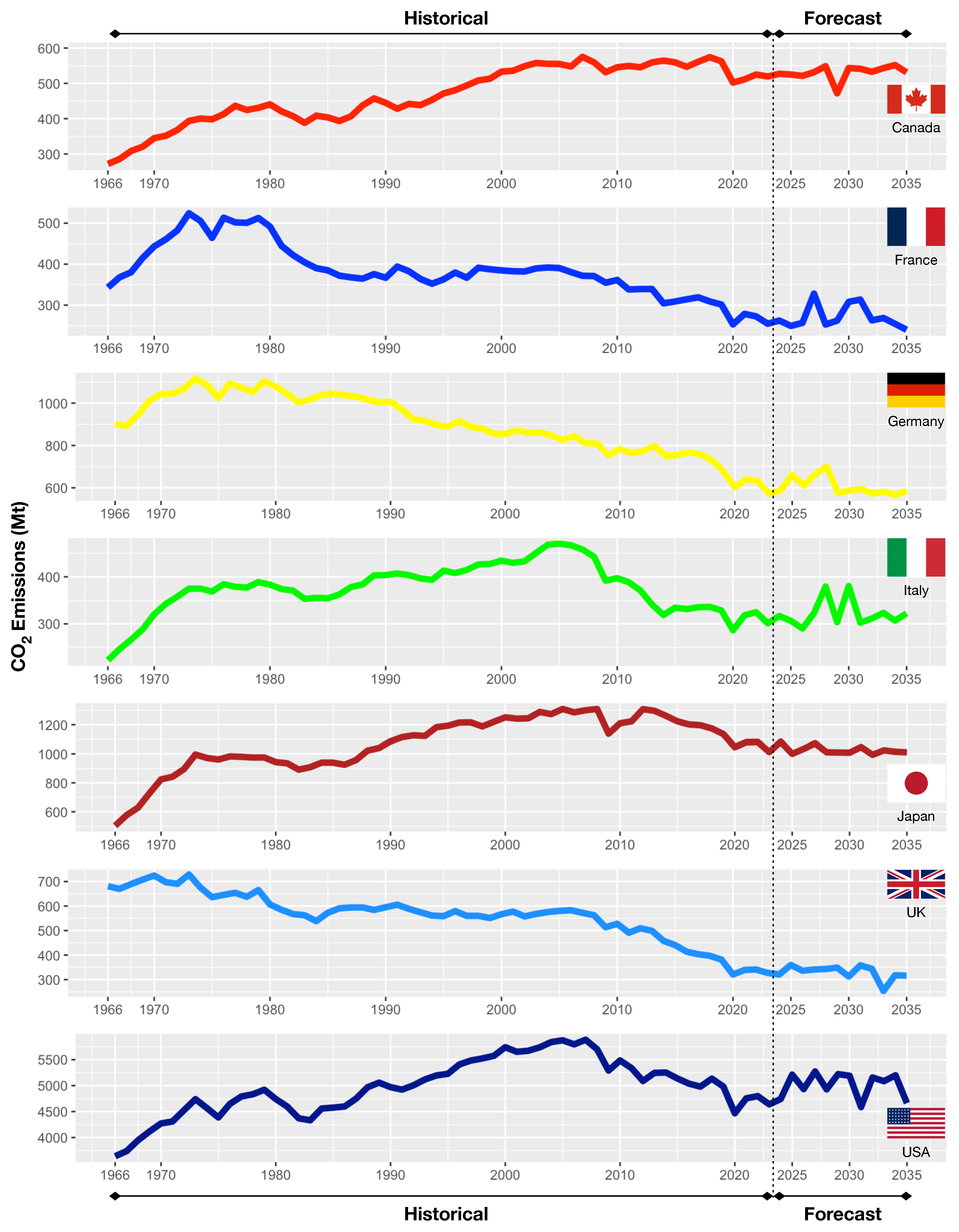
Furthermore, 1966–2023 historical and 2024–2035 forecast projections for CO₂ emission predictions of G7 countries are elucidated by the visualization in Figure 4. Here, CO₂ emissions in Mt are shown on the y-axis for each country and the years from 1966 to 2035 are illustrated on the x-axis as well.

According to Figure 4, Canada’s CO₂ emissions in 2023 were 519.50 Mt, will rise to 548.57 Mt by 2028, then will fluctuate and ascend to 551.86 Mt by 2034. France’s 2023 CO₂ emissions were 254.60 Mt, are expected to increase to 328.01 Mt and 313.53 Mt by 2027 and 2031 after some variations, and will eventually decrease to 254.32 Mt by 2034. Similarly, Germany’s CO₂ emissions in 2023 were 571.90 Mt, will reach 660.71 Mt and 700.03 Mt by 2025 and 2028, and will fall to 566.00 by 2034. Italy’s 2023 CO₂ emissions were 301.30 Mt, will oscillate and attain the values of 379.34 Mt and 380.52 Mt in 2028 and 2030, then will reduce to 306.75 Mt by 2034. Japan’s CO₂ emissions in 2023 were 1012.80 Mt, which will show slight fluctuations and stabilize around 1014.46 Mt in 2034. The UK’s 2023 CO₂ emissions were 327.30 Mt, which will decrease to 312.54 Mt and 253.60 Mt in 2030 and 2033, will increase to 317.75 Mt by 2034. The USA’s CO₂ emissions in 2023 were 4639.70 Mt, will be lowered to 4587.66 Mt after some significant oscillations, and then will reach 5199.62 Mt in 2034.

Consequently, future CO₂ emission predictions for the year 2035 are anticipated to be 531.07 Mt for Canada, 239.80 Mt for France, 585.35 Mt for Germany, 322.29 Mt for Italy, 1010.86 Mt for Japan, 315.98 Mt for the UK, and 4662.86 Mt for the USA, respectively. It should be noted that these values are point predictions obtained from deterministic GEP models, and no formal prediction or confidence intervals are provided; therefore, they should be interpreted as scenario-like projections conditional on the historical data patterns.

From a policy perspective, the projected declining or stabilizing paths for France, Japan, and the UK are broadly consistent with their early and stringent net-zero commitments, whereas the expected increases for Canada, Germany, Italy, and especially the USA underscore the challenges these countries face in aligning current trajectories with their declared carbon-neutrality targets. These scenario-like projections therefore provide a useful indication of where additional mitigation efforts and structural changes in the energy mix may be most urgently required within the G7.

A further limitation of the present analysis is that it does not include an explicit quantification of forecast uncertainty; the long-term projections up to 2035 are reported without confidence or prediction bands and therefore do not capture the full uncertainty associated with model instability and parameter sensitivity.

It should also be emphasized that all reported error metrics are computed under a direct multi-step forecasting strategy with a strictly chronological train/test split, ensuring a rigorous out-of-sample evaluation across all forecast horizons.

4. Conclusions

This article aims to forecast the CO₂ emissions of the G7 countries, and the proposed GEP algorithm was implemented in comparison with the simple GEP algorithm. In the meantime, the retrospective CO₂ emissions between the years 1966 and 2023 were utilized with the explanatory variables FFEC, GDPpc, HEC, NEC, PEC, REC, and TP. Moreover, the performance results were evaluated by the error metrics named as nMAE, nRMSE, and MAPE along with computational time. On average, the proposed GEP, enriched with higher-degree functions, achieved 26% lower nMAE, 24% lower nRMSE, and 27% lower MAPE than the simple GEP across the G7 countries while preserving essentially the same level of computational efficiency.

Based on the innovative findings of the current study, the following implications can be highlighted:

• To the best of the authors’ knowledge, the proposed GEP algorithm with additional high-degree functions (square, cube, quartic, and power) has not previously been applied to forecast the CO₂ emissions in the existing literature. The current study has bridged this gap by proposing a novel GEP algorithm with additional functions such as square, cube, quartic, and power functions.
• In this study, a data set covering 1966-2023 was employed. Thus, the impact of the COVID-19 pandemic and the conflict between Russia and Ukraine on CO₂ emissions was also implicitly reflected in the data.
• Both the simple and proposed GEP models have been observed to be quite successful in estimating CO₂ emissions. According to the averages of the G7 countries for both models, the proposed GEP models consistently yield substantially lower nMAE, nRMSE, and MAPE values than the simple GEP models.
• When the duration of both models is compared, the proposed GEP models exhibit only a marginal difference of 0.2 s in average runtime compared to the simple GEP models, indicating that the richer function set does not introduce any meaningful computational burden and can be applied to larger and higher-resolution data sets in future studies.
• CO₂ emissions are projected to increase by 2.2%, 2.4%, 7.0%, and 0.5% in Canada, Germany, Italy, and the USA, sequentially, and to decrease by 5.8%, 0.2%, and 3.5% in France, Japan, and the UK, accordingly when the values of the years 2023 and 2035 are compared. Additionally, it is considered that France will be the most successful country in reducing CO₂ emissions within the G7 countries, while Italy will be the least.

Despite these promising results, several limitations should be acknowledged. First, the forecasts up to 2035 are reported as point predictions without formal confidence or prediction intervals and thus should be interpreted with caution, especially in the presence of potential structural breaks due to policy changes or global shocks. Second, although multiple independent GEP runs were conducted to obtain empirical ranges of predicted values, a full probabilistic treatment of uncertainty (e.g., via bootstrap aggregation or Bayesian methods) is left for future work.

From a policy perspective, an important advantage of the proposed GEP approach is that it produces explicit, human-readable equations linking CO₂ emissions to key drivers such as fossil fuel energy consumption, renewable energy consumption, and GDP per capita. These equations can be directly embedded into national planning tools and scenario analyses without requiring complex software or black-box models, thereby supporting transparent and reproducible evidence-based decision-making for each G7 country.

From a practical standpoint, the explicit GEP equations derived for each G7 country can be directly integrated into national and regional planning tools to evaluate whether current emission trajectories are compatible with declared net-zero targets. In addition, these equations enable transparent scenario analyses under alternative assumptions for key drivers such as fossil-fuel and renewable energy consumption, thereby supporting evidence-based climate and energy policy design without the need for complex black-box models.

Future research could extend the proposed framework by incorporating additional socioeconomic and technological variables, applying the method to other country groups, and integrating formal uncertainty quantification to further enhance the robustness of long-horizon CO₂ emission forecasts.

References

1. Ofori, E.K.; Onifade, S.T.; Ali, E.B.; Alola, A.A.; Zhang, J. Achieving carbon neutrality in post COP26 in BRICS, MINT, and G7 economies: The role of financial development and governance indicators. J. Clean. Prod. 2023, 387, 135853. [Google Scholar] [CrossRef] [Scilit]
2. Ali, G.; Abbas, S.; Pan, Y.; Chen, Z.; Hussain, J.; Sajjad, M.; Ashraf, A. Urban environment dynamics and low carbon society: Multi-criteria decision analysis modeling for policy makers. Sustain. Cities Soc. 2019, 51, 101763. [Google Scholar] [CrossRef] [Scilit]
3. Capellán-Pérez, I.; de Castro, C.; Miguel González, L.J. Dynamic Energy Return on Energy Investment (EROI) and material requirements in scenarios of global transition to renewable energies. Energy Strategy Rev. 2019, 26, 100399. [Google Scholar] [CrossRef] [Scilit]
4. Wang, Q.; Wang, S. Is energy transition promoting the decoupling economic growth from emission growth? Evidence from the 186 countries. J. Clean. Prod. 2020, 260, 120768. [Google Scholar] [CrossRef] [Scilit]
5. US Environmental Protection Agency. 2022. Available online: https://www.epa.gov/ghgemissions/global-greenhouse-gas-emissions-data (accessed on 25 April 2026).
6. Wang, Z.; He, W.; Wang, B. Performance and reduction potential of energy and CO2 emissions among the APEC’s members with considering the return to scale. Energy 2017, 138, 552–562. [Google Scholar] [CrossRef] [Scilit]
7. Sun, W.; Wang, C.; Zhang, C. Factor analysis and forecasting of CO2 emissions in Hebei, using extreme learning machine based on particle swarm optimization. J. Clean. Prod. 2017, 162, 1095–1101. [Google Scholar] [CrossRef] [Scilit]
8. Fang, D.; Zhang, X.; Yu, Q.; Jin, T.C.; Tian, L. A novel method for carbon dioxide emission forecasting based on improved Gaussian processes regression. J. Clean. Prod. 2018, 173, 143–150. [Google Scholar] [CrossRef] [Scilit]
9. Liu, Z.; Li, D.; Zhang, J.; Saleem, M.; Zhang, Y.; Ma, R.; He, Y.; Yang, J.; Xiang, H.; Wei, H. Effect of simulated acid rain on soil CO2, CH4 and N2O emissions and microbial communities in an agricultural soil. Geoderma 2020, 366, 114222. [Google Scholar] [CrossRef] [Scilit]
10. Bakay, M.S.; Ağbulut, Ü. Electricity production based forecasting of greenhouse gas emissions in Turkey with deep learning, support vector machine and artificial neural network algorithms. J. Clean. Prod. 2021, 285, 125324. [Google Scholar] [CrossRef] [Scilit]
11. Tao, H.; Zhuang, S.; Xue, R.; Cao, W.; Tian, J.; Shan, Y. Environmental Finance: An Interdisciplinary Review. Technol. Forecast. Soc. Change 2022, 179, 121639. [Google Scholar] [CrossRef] [Scilit]
12. Ding, S.; Dang, Y.G.; Li, X.M.; Wang, J.J.; Zhao, K. Forecasting Chinese CO2 emissions from fuel combustion using a novel grey multivariable model. J. Clean. Prod. 2017, 162, 1527–1538. [Google Scholar] [CrossRef] [Scilit]
13. Chaudhry, S.M.; Ahmed, R.; Shafiullah, M.; Duc Huynh, T.L. The impact of carbon emissions on country risk: Evidence from the G7 economies. J. Environ. Manag. 2020, 265, 110533. [Google Scholar] [CrossRef] [Scilit]
14. Doğan, B.; Balsalobre-Lorente, D.; Nasir, M.A. European commitment to COP21 and the role of energy consumption, FDI, trade and economic complexity in sustaining economic growth. J. Environ. Manag. 2020, 273, 111146. [Google Scholar] [CrossRef] [Scilit]
15. Nasir, M.A.; Canh, N.P.; Lan Le, T.N. Environmental degradation & role of financialisation, economic development, industrialisation and trade liberalisation. J. Environ. Manag. 2021, 277, 111471. [Google Scholar] [CrossRef] [Scilit]
16. IPCC. Climate Change 2022: Impacts, Adaptation and Vulnerability; IPCC Sixth Assessment Report; Cambridge University Press: New York, NY, USA, 2022; Available online: https://www.ipcc.ch/report/ar6/wg2/ (accessed on 25 April 2026).
17. Karmellos, M.; Kosmadakis, V.; Dimas, P.; Tsakanikas, A.; Fylaktos, N.; Taliotis, C.; Zachariadis, T. A decomposition and decoupling analysis of carbon dioxide emissions from electricity generation: Evidence from the EU-27 and the UK. Energy 2021, 231, 120861. [Google Scholar] [CrossRef] [Scilit]
18. Ozdemir, A.C.; Buluş, K.; Zor, K. Medium- to long-term nickel price forecasting using LSTM and GRU networks. Resour. Policy 2022, 78, 102906. [Google Scholar] [CrossRef] [Scilit]
19. Shahbaz, M.; Kablan, S.; Hammoudeh, S.; Nasir, M.A.; Kontoleon, A. Environmental implications of increased US oil production and liberal growth agenda in post -Paris Agreement era. J. Environ. Manag. 2020, 271, 110785. [Google Scholar] [CrossRef] [Scilit]
20. Singh, H.; Najafi, M.R.; Cannon, A.J. Characterizing non-stationary compound extreme events in a changing climate based on large-ensemble climate simulations. Clim. Dyn. 2021, 56, 1389–1405. [Google Scholar] [CrossRef] [Scilit]
21. González-Torres, M.; Pérez-Lombard, L.; Coronel, J.; Maestre, I. Revisiting Kaya Identity to define an Emissions Indicators Pyramid. J. Clean. Prod. 2021, 317, 128328. [Google Scholar] [CrossRef] [Scilit]
22. WDI. World Development Indicators. 2024. Available online: https://databank.worldbank.org/source/world-development-indicators (accessed on 25 April 2026).
23. Huang, Y.; Haseeb, M.; Usman, M.; Ozturk, I. Dynamic association between ICT, renewable energy, economic complexity and ecological footprint: Is there any difference between E-7 (developing) and G-7 (developed) countries? Technol. Soc. 2022, 68, 101853. [Google Scholar] [CrossRef] [Scilit]
24. Murshed, M.; Saboori, B.; Madaleno, M.; Wang, H.; Doğan, B. Exploring the nexuses between nuclear energy, renewable energy, and carbon dioxide emissions: The role of economic complexity in the G7 countries. Renew. Energy 2022, 190, 664–674. [Google Scholar] [CrossRef] [Scilit]
25. Choudhari, V.; Dhoble, A.; Sathe, T. A review on effect of heat generation and various thermal management systems for lithium ion battery used for electric vehicle. J. Energy Storage 2020, 32, 101729. [Google Scholar] [CrossRef] [Scilit]
26. Pham, N.M.; Huynh, T.L.D.; Nasir, M.A. Environmental consequences of population, affluence and technological progress for European countries: A Malthusian view. J. Environ. Manag. 2020, 260, 110143. [Google Scholar] [CrossRef] [Scilit]
27. Zhou, W.; Zeng, B.; Wang, J.; Luo, X.; Liu, X. Forecasting Chinese carbon emissions using a novel grey rolling prediction model. Chaos Solitons Fractals 2021, 147, 110968. [Google Scholar] [CrossRef] [Scilit]
28. Liu, Z.; Jiang, P.; Wang, J.; Zhang, L. Ensemble system for short term carbon dioxide emissions forecasting based on multi-objective tangent search algorithm. J. Environ. Manag. 2022, 302, 113951. [Google Scholar] [CrossRef] [Scilit]
29. Qiao, W.; Lu, H.; Zhou, G.; Azimi, M.; Yang, Q.; Tian, W. A hybrid algorithm for carbon dioxide emissions forecasting based on improved lion swarm optimizer. J. Clean. Prod. 2020, 244, 118612. [Google Scholar] [CrossRef] [Scilit]
30. Wu, L.; Li, N.; Yang, Y. Prediction of air quality indicators for the Beijing-Tianjin-Hebei region. J. Clean. Prod. 2018, 196, 682–687. [Google Scholar] [CrossRef] [Scilit]
31. Lu, H.; Guo, L.; Azimi, M.; Huang, K. Oil and Gas 4.0 era: A systematic review and outlook. Comput. Ind. 2019, 111, 68–90. [Google Scholar] [CrossRef] [Scilit]
32. Lin, C.S.; Liou, F.M.; Huang, C.P. Grey forecasting model for CO2 emissions: A Taiwan study. Appl. Energy 2011, 88, 3816–3820. [Google Scholar] [CrossRef] [Scilit]
33. Pao, H.T.; Tsai, C.M. Modeling and forecasting the CO2 emissions, energy consumption, and economic growth in Brazil. Energy 2011, 36, 2450–2458. [Google Scholar] [CrossRef] [Scilit]
34. Pao, H.T.; Fu, H.C.; Tseng, C.L. Forecasting of CO2 emissions, energy consumption and economic growth in China using an improved grey model. Energy 2012, 40, 400–409. [Google Scholar] [CrossRef] [Scilit]
35. Aydın, G. The development and validation of regression models to predict energy-related CO2 emissions in Turkey. Energy Sources B Econ. Plan. Policy 2015, 10, 176–182. [Google Scholar] [CrossRef] [Scilit]
36. Wu, L.; Liu, S.; Liu, D.; Fang, Z.; Xu, H. Modelling and forecasting CO2 emissions in the BRICS (Brazil, Russia, India, China, and South Africa) countries using a novel multi-variable grey model. Energy 2015, 79, 489–495. [Google Scholar] [CrossRef] [Scilit]
37. Sun, W.; Liu, M. Prediction and analysis of the three major industries and residential consumption CO2 emissions based on least squares support vector machine in China. J. Clean. Prod. 2016, 122, 144–153. [Google Scholar] [CrossRef] [Scilit]
38. Wang, Z.X.; Ye, D.J. Forecasting Chinese carbon emissions from fossil energy consumption using non-linear grey multivariable models. J. Clean. Prod. 2017, 142, 600–612. [Google Scholar] [CrossRef] [Scilit]
39. Dai, S.; Niu, D.; Han, Y. Forecasting of Energy-Related CO2 Emissions in China Based on GM(1,1) and Least Squares Support Vector Machine Optimized by Modified Shuffled Frog Leaping Algorithm for Sustainability. Sustainability 2018, 10, 958. [Google Scholar] [CrossRef] [Scilit]
40. Hong, T.; Jeong, K.; Koo, C. An optimized gene expression programming model for forecasting the national CO2 emissions in 2030 using the metaheuristic algorithms. Appl. Energy 2018, 228, 808–820. [Google Scholar] [CrossRef] [Scilit]
41. Zhao, X.; Han, M.; Ding, L.; Liu, M. Forecasting carbon dioxide emissions based on a hybrid of mixed data sampling regression model and back propagation neural network in the USA. Environ. Sci. Pollut. Res. 2018, 25, 2899–2910. [Google Scholar] [CrossRef] [Scilit]
42. Heydari, A.; Garcia, D.A.; Keynia, F.; Bisegna, F.; Santoli, L.D. Renewable Energies Generation and Carbon Dioxide Emission Forecasting in Microgrids and National Grids using GRNN-GWO Methodology. Energy Procedia 2019, 159, 154–159. [Google Scholar] [CrossRef] [Scilit]
43. Hosseini, S.M.; Saifoddin, A.; Shirmohammadi, R.; Aslani, A. Forecasting of CO2 emissions in Iran based on time series and regression analysis. Energy Rep. 2019, 5, 619–631. [Google Scholar] [CrossRef] [Scilit]
44. Şahin, U. Forecasting of Turkey’s greenhouse gas emissions using linear and nonlinear rolling metabolic grey model based on optimization. J. Clean. Prod. 2019, 239, 118079. [Google Scholar] [CrossRef] [Scilit]
45. Zhu, B.; Ye, S.; Jiang, M.; Wang, P.; Wu, Z.; Xie, R.; Chevallier, J.; Wei, Y.M. Achieving the carbon intensity target of China: A least squares support vector machine with mixture kernel function approach. Appl. Energy 2019, 233-234, 196–207. [Google Scholar] [CrossRef] [Scilit]
46. Ofosu-Adarkwa, J.; Xie, N.; Javed, S.A. Forecasting CO2 emissions of China’s cement industry using a hybrid Verhulst-GM(1,N) model and emissions’ technical conversion. Renew. Sust. Energ. Rev. 2020, 130, 109945. [Google Scholar] [CrossRef] [Scilit]
47. Wu, W.; Ma, X.; Zhang, Y.; Li, W.; Wang, Y. A novel conformable fractional non-homogeneous grey model for forecasting carbon dioxide emissions of BRICS countries. Sci. Total Environ. 2020, 707, 135447. [Google Scholar] [CrossRef] [Scilit] [PubMed]
48. Guo, J.; Liu, W.; Tu, L.; Chen, Y. Forecasting carbon dioxide emissions in BRICS countries by exponential cumulative grey model. Energy Rep. 2021, 7, 7238–7250. [Google Scholar] [CrossRef] [Scilit]
49. Nguyen, D.K.; Huynh, T.L.D.; Nasir, M.A. Carbon emissions determinants and forecasting: Evidence from G6 countries. J. Environ. Manag. 2021, 285, 111988. [Google Scholar] [CrossRef] [Scilit]
50. Qiao, Z.; Meng, X.; Wu, L. Forecasting carbon dioxide emissions in APEC member countries by a new cumulative grey model. Ecol. Indic. 2021, 125, 107593. [Google Scholar] [CrossRef] [Scilit]
51. Tong, M.; Duan, H.; He, L. A novel Grey Verhulst model and its application in forecasting CO2 emissions. Environ. Sci. Pollut. Res. 2021, 28, 31370–31379. [Google Scholar] [CrossRef] [Scilit] [PubMed]
52. Xu, Z.; Liu, L.; Wu, L. Forecasting the carbon dioxide emissions in 53 countries and regions using a non-equigap grey model. Environ. Sci. Pollut. Res. 2021, 28, 15659–15672. [Google Scholar] [CrossRef] [Scilit]
53. Faruque, M.O.; Rabby, M.A.J.; Hossain, M.A.; Islam, M.R.; Rashid, M.M.U.; Muyeen, S. A comparative analysis to forecast carbon dioxide emissions. Energy Rep. 2022, 8, 8046–8060. [Google Scholar] [CrossRef] [Scilit]
54. Kour, M. Modelling and forecasting of carbon-dioxide emissions in South Africa by using ARIMA model. Int. J. Environ. Sci. Technol. 2022, 74. [Google Scholar] [CrossRef] [Scilit]
55. Ağbulut, Ü. Forecasting of transportation-related energy demand and CO2 emissions in Turkey with different machine learning algorithms. Sustain. Prod. Consum. 2022, 29, 141–157. [Google Scholar] [CrossRef] [Scilit]
56. Karakurt, I.; Aydin, G. Development of regression models to forecast the CO2 emissions from fossil fuels in the BRICS and MINT countries. Energy 2023, 263, 125650. [Google Scholar] [CrossRef] [Scilit]
57. Yin, F.; Bo, Z.; Yu, L.; Wang, J. Prediction of carbon dioxide emissions in China using a novel grey model with multi-parameter combination optimization. J. Clean. Prod. 2023, 404, 136889. [Google Scholar] [CrossRef] [Scilit]
58. Iftikhar, H.; Khan, M.; Żywiołek, J.; Khan, M.; López-Gonzales, J.L. Modeling and forecasting carbon dioxide emission in Pakistan using a hybrid combination of regression and time series models. Heliyon 2024, 10, e33148. [Google Scholar] [CrossRef] [Scilit]
59. Ding, S.; Ye, J.; Cai, Z. Multi-step carbon emissions forecasting using an interpretable framework of new data preprocessing techniques and improved grey multivariable convolution model. Technol. Forecast. Soc. Chang. 2024, 208, 123720. [Google Scholar] [CrossRef] [Scilit]
60. Yang, W.; Qiao, Z.; Wu, L.; Ren, X.; Taghizadeh-Hesary, F. Forecasting carbon dioxide emissions using adjacent accumulation multivariable grey model. Gondwana Res. 2024, 134, 107–122. [Google Scholar] [CrossRef] [Scilit]
61. Noman, E.A.; Al-Gheethi, A.A.; Radin Maya Saphira, R.M.; Talip, B.A.; Al-Sahari, M.; Ismail, N. Mathematical prediction models for inactivation of antibiotic-resistant bacteria in kitchen wastewater by bimetallic bionanoparticles using machine learning with gene expression programming. J. Clean. Prod. 2022, 333, 130131. [Google Scholar] [CrossRef] [Scilit]
62. Shishegaran, A.; Saeedi, M.; Kumar, A.; Ghiasinejad, H. Prediction of air quality in Tehran by developing the nonlinear ensemble model. J. Clean. Prod. 2020, 259, 120825. [Google Scholar] [CrossRef] [Scilit]
63. Zhang, L.; Li, Z.; Królczyk, G.; Wu, D.; Tang, Q. Mathematical modeling and multi-attribute rule mining for energy efficient job-shop scheduling. J. Clean. Prod. 2019, 241, 118289. [Google Scholar] [CrossRef] [Scilit]
64. Energy & Climate Intelligence Unit. Net Zero Emissions Race, 2024 Scorecard. Available online: https://eciu.net/netzerotracker (accessed on 25 April 2026).
65. Ahmadi, M.H.; Jashnani, H.; Chau, K.W.; Kumar, R.; Rosen, M.A. Carbon dioxide emissions prediction of five Middle Eastern countries using artificial neural networks. Energy Sources Part A Recover. Util. Environ. Eff. 2019, 45, 9513–9525. [Google Scholar] [CrossRef] [Scilit]
66. BP. Statistical Review of World Energy. Available online: https://www.bp.com/en/global/corporate/energy-economics/statistical-review-of-world-energy.html (accessed on 25 April 2026).
67. Desgagné, A.; de Micheaux, P.L. A powerful and interpretable alternative to the Jarque–Bera test of normality based on 2nd-power skewness and kurtosis, using the Rao’s score test on the APD family. J. Appl. Stat. 2018, 45, 2307–2327. [Google Scholar] [CrossRef] [Scilit]
68. Ostrom, W.C. Time Series Analysis: Regression Techniques; Sage: Thousand Oaks, CA, USA, 1990; Volume 9. [Google Scholar]
69. Castillo, F.A.; Villa, C.M. Symbolic regression in multicollinearity problems. In Proceedings of the 7th Annual Conference on Genetic and Evolutionary Computation, GECCO ’05, Washington, DC, USA, 25–29 June 2005; pp. 2207–2208. [Google Scholar] [CrossRef] [Scilit]
70. Patil, I. Visualizations with statistical details: The ‘ggstatsplot’ approach. J. Open Source Softw. 2021, 6, 3167. [Google Scholar] [CrossRef] [Scilit]
71. Ferreira, C. Gene Expression Programming: A New Adaptive Algorithm for Solving Problems. arXiv 2001, arXiv:cs/0102027. [Google Scholar] [CrossRef] [Scilit]
72. Zor, K.; Çelik, Ö.; Timur, O.; Teke, A. Short-Term Building Electrical Energy Consumption Forecasting by Employing Gene Expression Programming and GMDH Networks. Energies 2020, 13, 1102. [Google Scholar] [CrossRef] [Scilit]
73. Çelik, O.; Zor, K.; Tan, A.; Teke, A. A novel gene expression programming-based MPPT technique for PV micro-inverter applications under fast-changing atmospheric conditions. Sol. Energy 2022, 239, 268–282. [Google Scholar] [CrossRef] [Scilit]
74. Tolun, G.G.; Zor, K. Very Short-Term Reactive Power Forecasting Using Machine Learning-Based Algorithms. In Proceedings of the 2024 9th International Youth Conference on Energy (IYCE), Colmar, France, 2–6 July 2024; pp. 1–5. [Google Scholar] [CrossRef] [Scilit]
75. Tolun, G.G.; Tolun, Ö.C.; Zor, K. An Application of Prosumer Electric Load Forecasting with Machine Learning-Based Algorithms. In Proceedings of the 2024 15th National Conference on Electrical and Electronics Engineering (ELECO), Bursa, Türkiye, 28–30 November 2024; pp. 1–6. [Google Scholar] [CrossRef] [Scilit]
76. Liu, Y. gepR: Composite Linear-Nonlinear Regression Using GEP. R Package Version. 2018. Available online: https://github.com/profyliu/gepR (accessed on 25 April 2026).
77. Kuhn, M. Building Predictive Models in R Using the caret Package. J. Stat. Softw. 2008, 28, 1–26. [Google Scholar] [CrossRef] [Scilit]
78. Wickham, H. ggplot2: Elegant Graphics for Data Analysis; Springer: New York, NY, USA, 2016. [Google Scholar]
79. Atalay, B.A.; Zor, K. An Innovative Approach for Forecasting Hydroelectricity Generation by Benchmarking Tree-Based Machine Learning Models. Appl. Sci. 2025, 15, 10514. [Google Scholar] [CrossRef] [Scilit]
80. Cebeci, C.; Zor, K. Electricity Demand Forecasting Using Deep Polynomial Neural Networks and Gene Expression Programming During COVID-19 Pandemic. Appl. Sci. 2025, 15, 2843. [Google Scholar] [CrossRef] [Scilit]
81. Tolun, O.C.; Zor, K.; Tutsoy, O. A comprehensive benchmark of machine learning-based algorithms for medium-term electric vehicle charging demand prediction. J. Supercomput. 2025, 81, 475. [Google Scholar] [CrossRef] [Scilit]
82. Zor, K.; Gizem Tolun, G.; Zor, E.Ş. Forecasting Electricity Generation of a Geothermal Power Plant Using LSTM and GRU Networks. In Proceedings of the 2025 7th Global Power, Energy and Communication Conference (GPECOM), Bochum, Germany, 11–13 June 2025; pp. 531–536. [Google Scholar] [CrossRef] [Scilit]
83. Zhou, C.; Chen, X. Predicting China’s energy consumption: Combining machine learning with three-layer decomposition approach. Energy Rep. 2021, 7, 5086–5099. [Google Scholar] [CrossRef] [Scilit]
Figure 2. Methodological framework of the proposed approach. The diagram summarizes the main steps of the study: (i) data wrangling and construction of the clean data set, including chronological 80/20 train–test splitting and min–max normalization; (ii) model development using the Simple GEP (with five basic functions) and the proposed GEP (with an enriched function set including square, cube, quartic, and power operators); and (iii) direct multi-step forecasting of CO2 emissions for the G7 countries for the horizons 2024–2035, together with the computation of accuracy metrics (nMAE, nRMSE, MAPE) and runtime.
Applsci 16 04676 g002
Figure 3. Visualization of a sample expression tree generated by the GEP algorithm. Nodes correspond to functions (e.g., the square-root operator Q) and terminals (input variables or constants), and the tree encodes the symbolic regression equation shown in Table 5. The figure illustrates how a fixed-length linear chromosome is decoded into a non-linear analytical formula within the GEP framework, providing interpretable relationships between the inputs and the target CO2 emissions.
Applsci 16 04676 g003
Figure 4. Historical and forecasted CO2 emissions for the G7 countries. For each country (Canada, France, Germany, Italy, Japan, the United Kingdom, and the United States), solid lines depict observed annual CO2 emissions (1966–2023), while dashed lines show point forecasts for 2024–2035 obtained from the proposed GEP model. Emissions are expressed in million tons (Mt). The figure highlights cross-country differences in historical emission trajectories and projected future paths and should be interpreted as scenario-like projections, since no formal prediction or confidence intervals are reported around the forecasts.
Applsci 16 04676 g004