A Deep Learning Framework for Full-Field Thermal Field Distribution Prediction from Digital Image Correlation Strain Measurements

Featured Application

This contribution shows that full-field thermal maps can be constructed directly from Digital Image Correlation (DIC) effective strain images using a supervised trained U-Net model. When the network is trained with sufficient data, it can later be used to predict thermal fields without the need for an infrared camera, given the prior training per use case, i.e., three-point bending, tensile testing, etc. This approach can simplify the experimental setup by allowing thermal fields to be obtained even when an infrared camera cannot be used. It is particularly useful in high-speed tests, setups where access for thermal imaging is restricted or impossible, or in laboratories lacking the necessary thermal-imaging infrastructure. In these situations, this method offers a practical way to estimate the relevant thermal response using only DIC measurements.

Abstract

Digital Image Correlation (DIC) and infrared thermography (IRT) are widely used for full-field experimental analysis of materials and structures; however, direct thermal measurements are often constrained by limited access, thermally opaque safety enclosures, or the availability of infrared equipment. This study presents a deep learning-based framework for predicting full-field temperature distributions directly from a DIC-derived effective strain field. A supervised U-Net regression model was trained on paired effective strain–temperature data obtained from high-speed three-point bending experiments on aluminum specimens. The network learns a direct mapping between effective strain fields and corresponding temperature fields without requiring explicit thermomechanical modelling. The model’s performance was evaluated on an independent test set using RMSE, MAE, SSIM, and the coefficient of determination. The proposed framework achieved a coefficient of determination of up to R² = 0.985 and showed strong spatial agreement with measured temperature fields, particularly during highly mechanically active deformation stages. These results demonstrate that reliable full-field temperature distributions can be reconstructed solely from strain measurements, providing a practical alternative to infrared thermography in experimental configurations where thermal imaging is impractical or unavailable.

1. Introduction

Digital Image Correlation (DIC) and infrared thermography (IRT) are common non-destructive testing techniques used for experimental analysis of materials and structures. DIC provides full-field displacement and strain distributions with high spatial resolution and has become a standard tool for analyzing deformation and damage evaluation [1,2,3]. In this work, DIC fields were computed and evaluated using NCorr, an open-source 2D DIC software widely adopted in the experimental mechanics community for accurate displacement and strain evaluation [4]. Infrared thermography, on the other hand, measures surface temperature distributions and is sensitive to local processes such as plastic dissipation, friction heating, crack growth, or thermal softening [5,6,7]. When these two methods are combined, researchers obtain a more complete picture of thermomechanical behaviour, especially during dynamic loading, fracture initiation, or fatigue testing.

However, IR thermography requires specialized instruments that are not easily justified for occasional use, and they also require calibration and are sensitive to reflections, ambient light, and environmental noise [5,8]. Additionally, they require a direct line of sight to the specimen, which is not always possible. A common example is high-energy impact testing or very-high-strain tests using a drop tower machine or split Hopkinson bar [9]. In many laboratories, safety regulations require the specimen to be placed inside a protective enclosure made from acrylic, polycarbonate, or tempered glass. These transparent shields protect the operator from fragments during impact but are IR-opaque [8]. DIC, however, can still function normally through such transparent windows, while infrared cameras cannot record correct temperature fields. As a result, only mechanical deformation data is available, and the thermal information is missing. In previous work, similarities of infrared (IR) image patterns and effective strain distributions obtained by DIC were described by Krstulović-Opara et al. [10], suggesting that the spatial structure of thermal and mechanical fields is strongly correlated during dynamic deformation.

Because of these limitations, a method that can estimate temperature fields from strain measurements alone would be extremely useful. With such a method, a researcher could still obtain thermomechanical insights even when thermography cannot be used due to safety barriers, optical restrictions, or budget limitations.

Recent developments in deep learning show that convolutional neural networks (CNNs) can learn complex mappings between different image datasets. Encoder–decoder architectures such as U-Net have demonstrated strong performance in segmentation, denoising, and general pixel-wise prediction tasks [7,11,12]. U-Net, originally introduced for biomedical imaging, combines multi-scale encoding with skip connections to preserve spatial detail [7]. These architectures are well suited for learning relationships between physical fields, provided that a sufficiently large, paired dataset exists, of which this is the first. Although image-to-image translation is well explored (e.g., pix2pix [13] and Cycle GAN [14]), very few studies attempt to predict thermal fields directly from DIC strain data. Still, mechanical deformation and thermal response are coupled through plastic dissipation, viscoelastic heating and other mechanisms [6,15,16]. Therefore, with enough paired examples, a neural network can learn this mapping and reconstruct temperature distributions even when no infrared camera is used—such as in the drop-tower case described earlier.

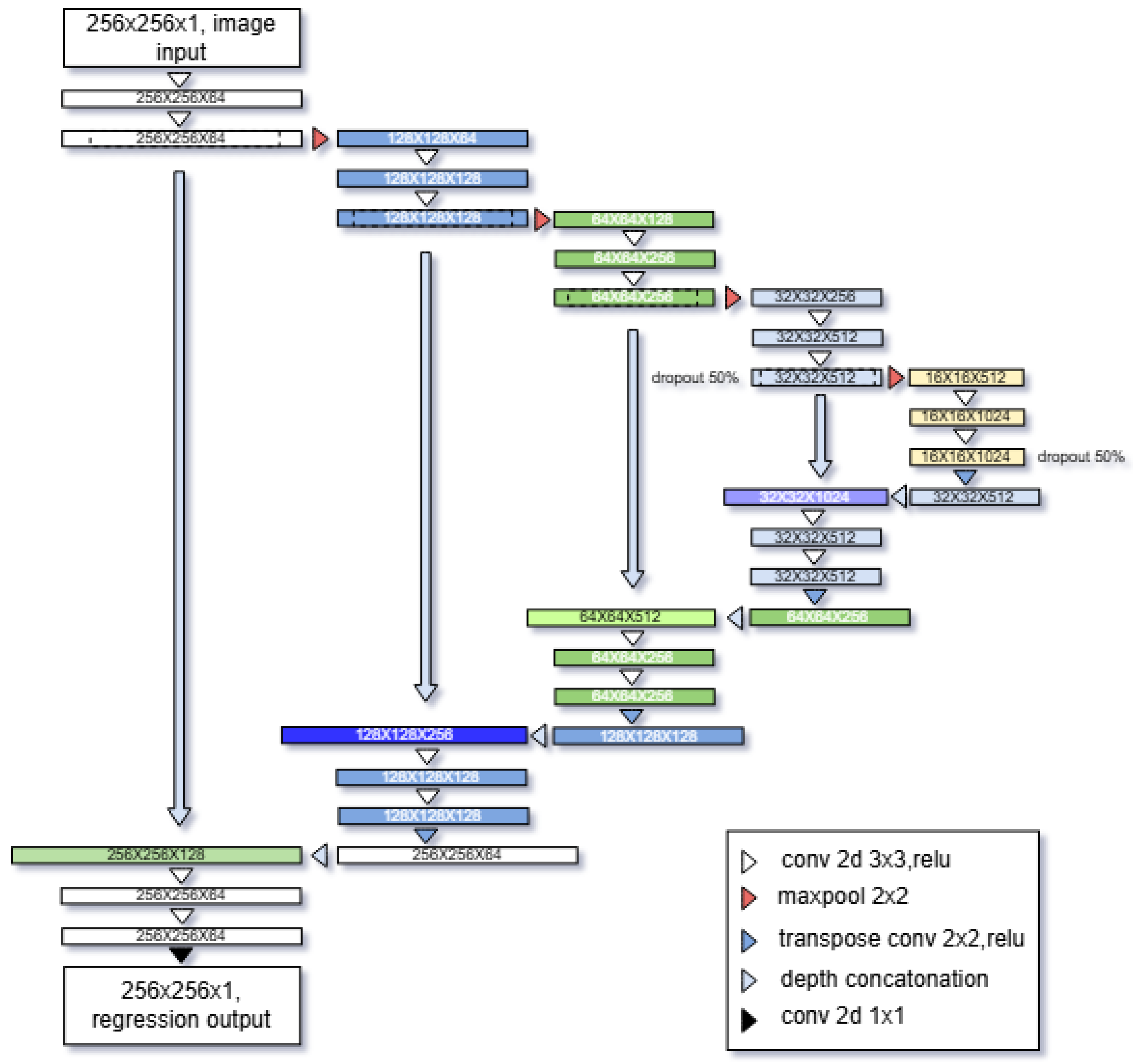
In this work, we present a U-Net-based deep regression model that predicts full-field thermal maps from DIC strain images. A custom dataset of paired strain–temperature fields was collected and processed using normalization and paired geometric augmentations. The U-Net architecture was modified to perform continuous regression, and several training strategies were designed to preserve the physical meaning of the data. Our results show that, when trained on a sufficiently representative dataset, the model can reconstruct thermal fields with high correlation and low error, demonstrating that thermography-free thermal estimation is feasible and practical.

2. Experimental Setup, Data Acquisition and Data Processing

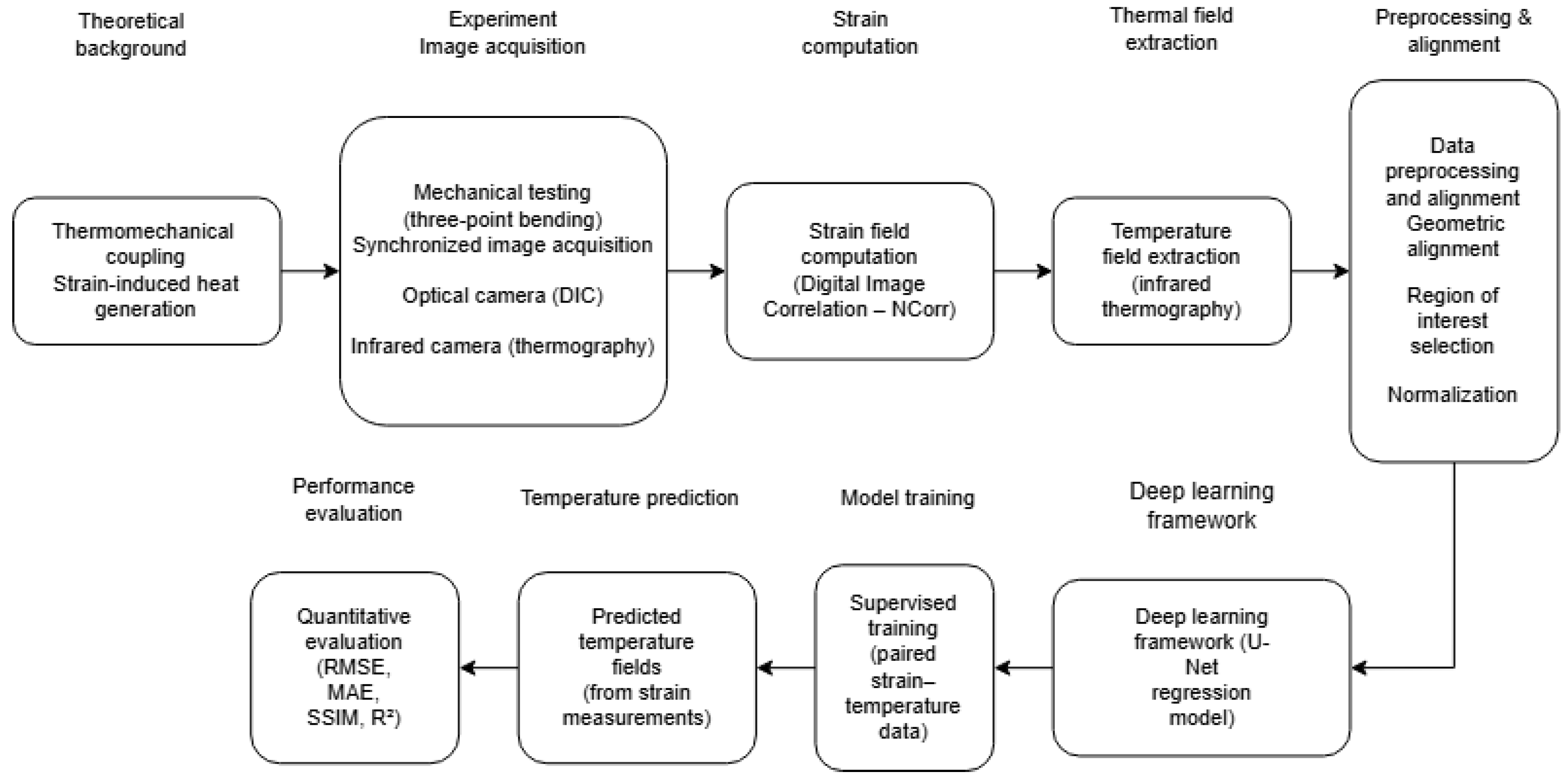
Before the paired DIC–thermal dataset could be used for training, the experiment and the measurement equipment had to be carefully designed to ensure that both deformation and temperature fields were acquired/recorded with sufficient quality. The overall research workflow of the proposed framework is summarized in Figure 1.

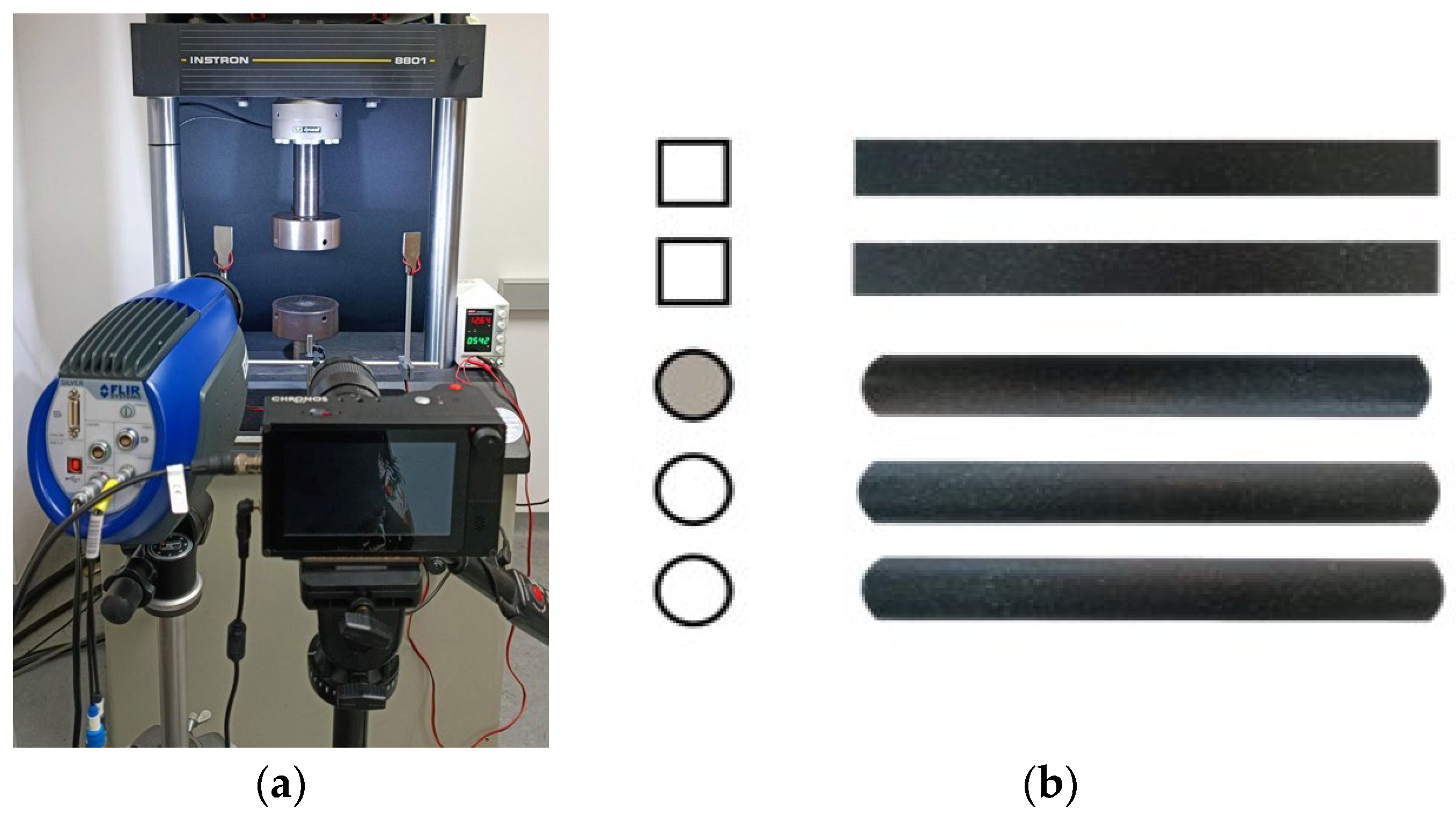
This section gives an overview of the testing configuration, the imaging systems (Figure 2a) used in the study, and the procedure for calculating strain based on high-speed images. In addition, several processing steps were required to convert the recorded images into a consistent and usable form for the neural network. The following subsections describe the data acquisition process and the steps applied for processing and augmenting the dataset.

2.1. Experimental Setup and Data Acquisition

The goal of this research was to demonstrate that thermal fields can be reconstructed directly from strain measurements even during rapid and strongly dynamic loading conditions. To ensure clear thermomechanical activity, the three-point bending test was chosen because of its highly predictable deformation pattern [10,17,18]. The test was performed on an Instron 8801 Servo hydraulic dynamic testing system at jaw separation speed of 287 mm/s. The infrared and optical cameras were mounted on two independent stands and positioned in a vertical, coaxial arrangement, with the infrared camera located below and the high-speed optical camera positioned directly above it. The housing of the optical camera was placed approximately 2 mm above the thermal camera housing to avoid thermal interference, while maintaining an unobstructed field of view of the same planar specimen surface. The optical camera was positioned at an approximate working distance of 1 m from the specimen, and both cameras remained fixed throughout the experiments. The optical axes of the two cameras were nearly parallel, with a small in-plane angular offset of approximately 1–2° measured via the fixture.

Fast loading promotes pronounced thermomechanical coupling, including thermoelastic effects and plastic dissipation, which become visible in infrared recordings [6,10]. In contrast, quasi-static tests at very low displacement rates (e.g., 0.1 mm/s) tend to equalize the surface temperature between frames due to heat dissipation, reducing observable gradients and making the thermal response less suitable for supervised learning. Thermal data were acquired using the cooled InSb Flir SC5000MW series infrared camera, operating at 320 × 256 pixels and 487 frames per second with emissivity coefficient 0.95. High-speed infrared imaging inherently involves trade-offs between frame rate and spatial resolution due to detector readout limits [5,15]. The selected frame rate provided adequate temporal resolution for dynamic thermography while preserving sufficient thermal detail. Simultaneously, mechanical deformation was captured using a Chronos 1.4 high-speed camera at 1280 × 1024 pixels and 487 frames per second, ensuring that both cameras remained synchronized. In addition, specimens were coated with black paint and sprayed with random speckled pattern for DIC [1,19]. Triggering of the two systems was coordinated using a custom-built trigger box that was manually activated prior to the start of the Instron test. Manual triggering was adopted due to differences between the trigger-out signal of the testing machine and the trigger-in requirements of the IR and high-speed cameras. A total of five specimens were tested under identical conditions undergoing a three-point bending test which ensured a predictable deformation region [10,17,18]. Specimens consisted of square and circular aluminum tubes, with one specimen filled with Ethylene–Vinyl Acetate to introduce a small amount of structural support and, therefore, variety in the dataset (see Figure 2b). The synchronized thermal and high-speed optical recordings formed the basis for constructing the paired DIC–thermal dataset used in this study.

2.2. Data Processing, Normalization, and Augmentation

The raw data obtained from the experiments consisted of full-frame DIC recordings from the high-speed optical system and temperature fields extracted from the infrared camera. Before the images could be used for network training, both datasets required several processing steps to obtain spatially aligned, normalized and sufficiently large datasets. The following subsections describe the procedures for DIC and thermal data separately, followed by the data preprocessing and augmentation strategy applied to both.

2.2.1. Digital Image Correlation Data Processing

The DIC-derived effective strain fields were treated as the geometric reference and were not modified, such that all geometric alignment operations were applied exclusively to the infrared data. The high-speed optical recordings were first processed in NCorr [4] to obtain displacement and strain fields. The settings used to acquire DIC from each individual datasets are shown in

Table 1. NCorr analysis parameters used for each dataset.

#	Frames Used in Analysis	Subset Radius	Subset Spacing	Num Threads	Diff Norm	Iterations	High Strain Analysis Leapfrog Number of Steps	Discontinues Analysis	Strain Radius
1	47	16	0	4	0.0001	99	5	On	10
2	55	15	0	4	0.001	99	3	On	10
3	36	17	0	4	0.001	99	7	On	10
4	34	15	0	4	0.0001	99	6	On	10
5	46	16	0	4	0.0001	50	Off auto-propagation option	On	10

. The subset radius sets the pixel size of each correlation window and determines how much image texture is used for tracking, while the subset spacing controls the distance between neighbouring points and, therefore, the spatial resolution of the displacement grid. The number of threads specifies how many CPU cores are used during processing. Convergence of the correlation is governed by the difference norm, which measures the change between iterations, and by the maximum number of iterations allowed for each subset. For cases involving large deformation, the high-strain leapfrog number of steps defines how many intermediate tracking steps NCorr introduces to maintain correlation stability. The discontinuous analysis option enables the algorithm to handle cracks or separations by permitting decorrelation when continuity breaks down. Finally, the strain radius controls the neighbourhood size used for polynomial fitting when computing strain fields, influencing the smoothness of the resulting strain maps [4].

NCorr calculates both the in-plane Green–Lagrange strain tensor, which does not move with the object [20], and the Eulerian–Almansi strain tensor, which is evaluated in the deformed configuration [20]. For our purposes, Eulerian–Almansi strain tensor components were chosen as the strain moves with the object during deformation [20].

$$E=\left[\begin{array}{cc}{E}_{xx}& E_{xy}\\ E_{yx}& E_{yy}\end{array}\right]$$

(1)

where E_xx is the normal strain in the x-direction, E_yy is the normal strain in the y-direction, and E_xy and E_yx represent the shear strain. They are used to describe in-plane deformation, as only one camera was used. From the normal and shear components, two principal strains were calculated, E₁ and E₂, which are eigenvalues of the matrix E (see Equation (1)) [20].

$$E_{\mathrm{1,2}}={\displaystyle \frac{E_{xx}+E_{yy}}{2}}\pm \sqrt{{\left({\displaystyle \frac{E_{xx}-E_{yy}}{2}}\right)}^2+{E_{xy}}^2}$$

(2)

An effective (von Mises-type) strain was adopted as a scalar invariant measure of deformation [20].

$$E_{eff}=\sqrt{{\displaystyle \frac{2}{3}}\left({\left(E_1-E_2\right)}^2+{E_1}^2+{E_2}^2\right)}$$

(3)

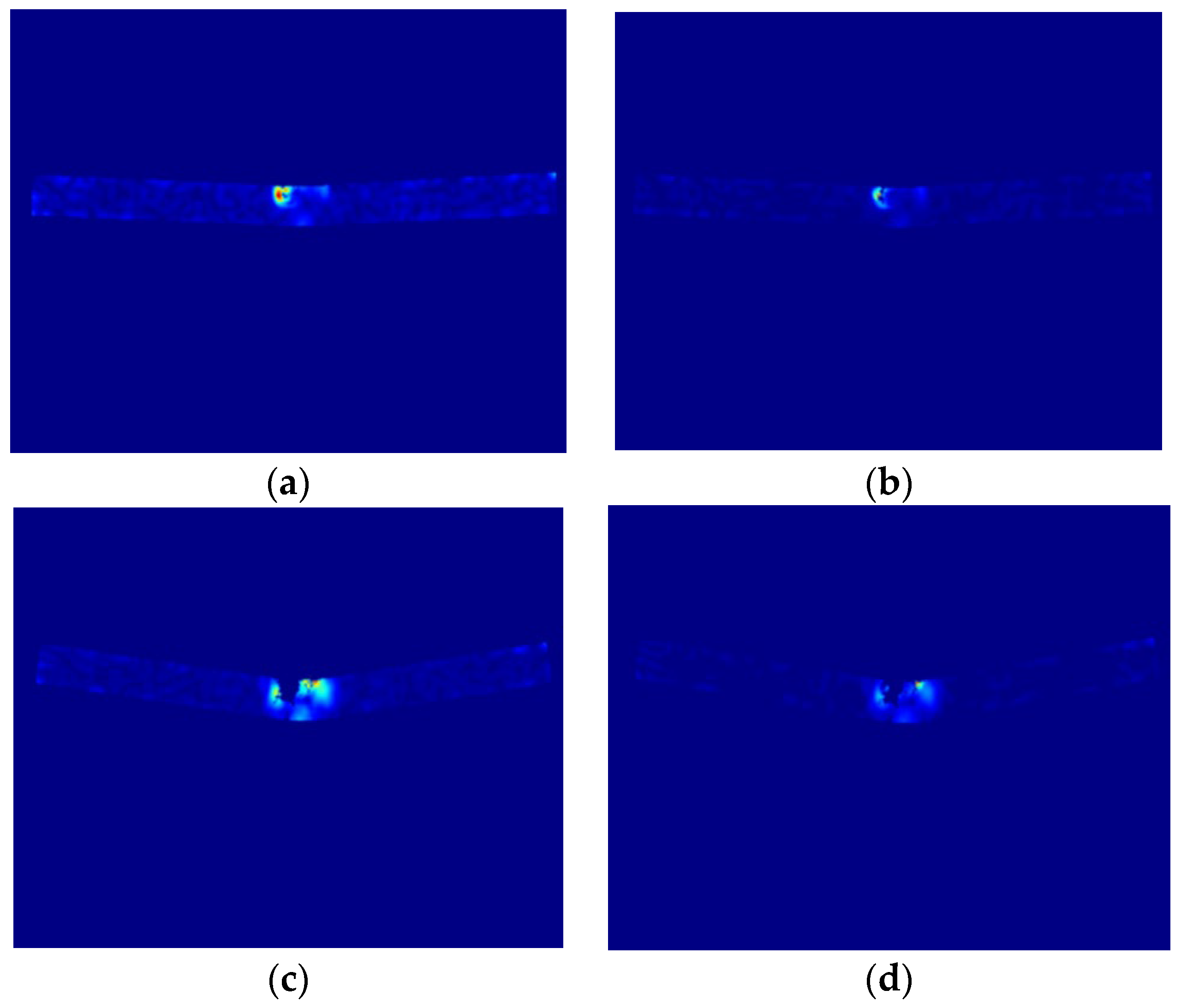
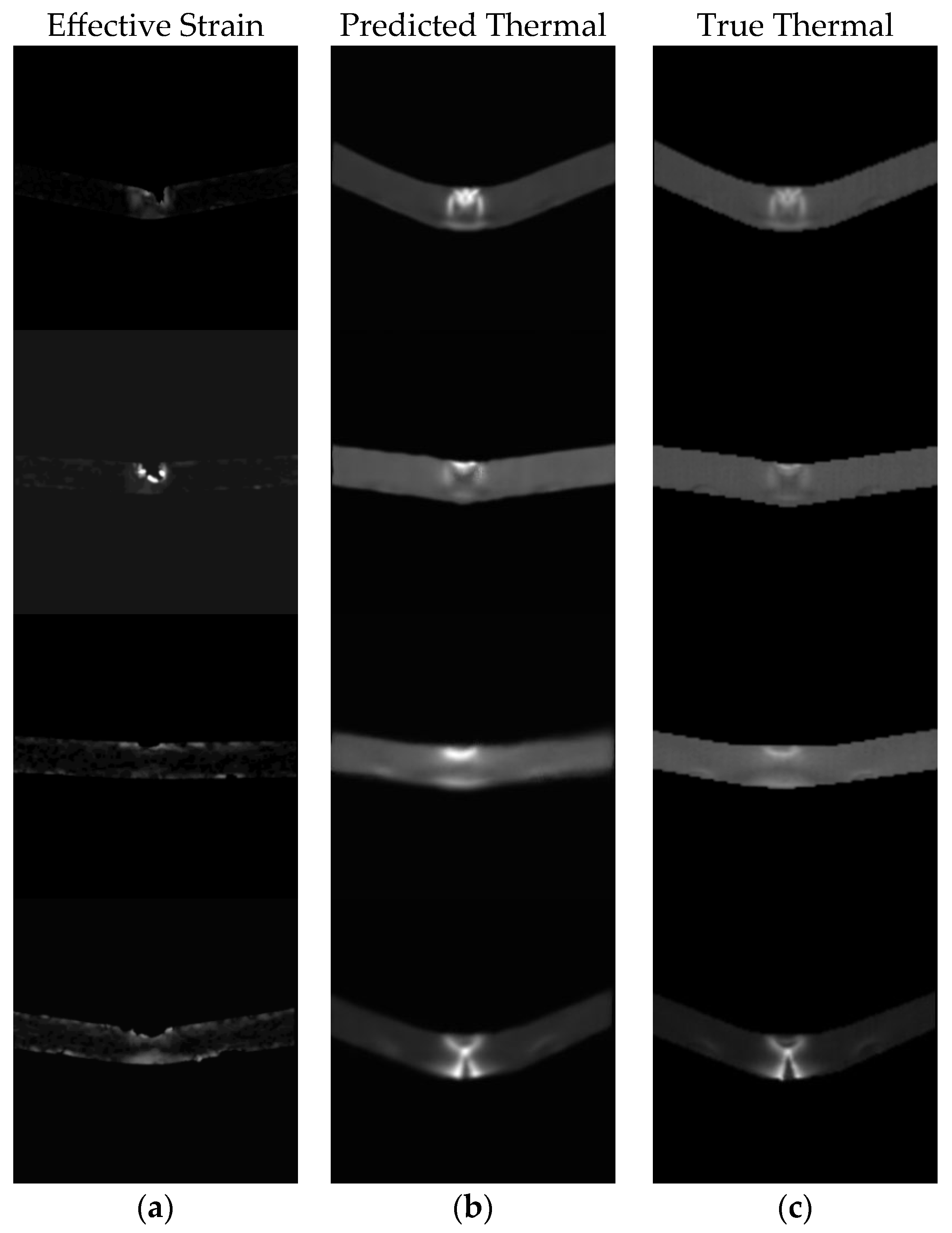
Owing to its definition in terms of the deviatoric strain tensor, the effective strain is directly related to plastic deformation and the associated energy dissipation. Therefore, effective strain is expected to show a strong correlation with temperature changes observed by infrared thermography [16]. In addition, the use of a scalar strain measure reduces the sensitivity to local fluctuations of principal strain directions and provides improved numerical robustness compared to individual principal strain components, which proved advantageous for deep learning-based image-to-field translation. Several frames from separate datasets and loading stages can be seen in the Figure 3.

2.2.2. Infrared Camera Data Processing

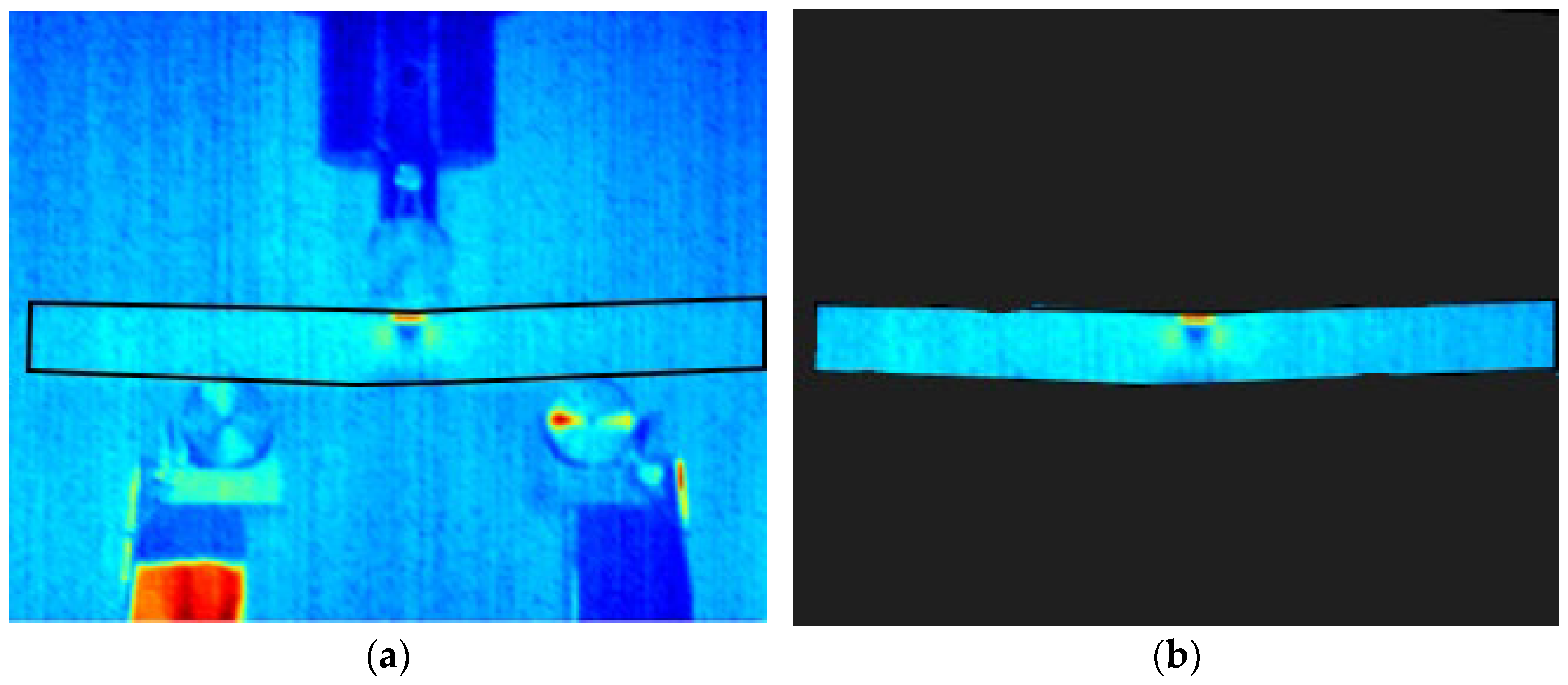
The infrared camera records data in the proprietary FLIR format, and each frame was subsequently exported as an ASCII matrix of temperature values. To ensure that only the specimen region was used for training, a bounding box was created around the specimen based on its visible outline. Everything outside this bounding box was excluded (see Figure 4), which removed the laboratory background, fixtures, and reflections that would otherwise degrade learning. Preliminary training was also performed using infrared images that included the full background; however, this configuration led to inferior performance, since the network was required to learn a more complex mapping from specimen-only DIC fields to thermal images containing both the specimen and surrounding background.

During the experiment, the thermal frames were recorded at a resolution of 320 × 256 pixels, which is approximately square but still includes unavoidable peripheral regions outside the specimens. Prior to cropping, a small in-plane rotation was applied only to the infrared frames to compensate for the measured angular offset between the infrared and optical cameras. Each frame was therefore cropped to a 256 × 256 pixel region centred on the specimen, ensuring spatial consistency with the processed DIC frames.

2.2.3. Data Processing

Both DIC-based strain fields and thermal images contained numerical artifacts that needed to be removed before the dataset could be used for training. These artifacts appeared as isolated pixels or small clusters showing unrealistically high values that were not physically possible for the given loading conditions. The problem is common in full-field numerical techniques: in DIC, it usually originates from local decorrelation or subset tracking failure [1,2], while in infrared measurements it is often caused by sensor noise or transient reflections [15].

To address these issues, a dedicated processing procedure was implemented in MATLAB 2022b and applied identically to all datasets of DIC strain and thermographic fields. For each frame, the following steps were executed:

1.

Outlier Detection.

   

Each image (DIC effective strain or thermal field) was scanned for large outlier values using a threshold-based rule. Thresholds were not universal; instead, they were chosen based on the expected physical of values possible in datasets.

a.

For DIC effective strain, values above an upper bound, e.g., >15% of maximum strain per image were flagged because such magnitudes should occur in the tested specimens.

b.

For the thermal fields, values outside the physically possible temperature range for the experiment were identified in the same way.

   

The algorithm produced a list of outlier pixel coordinates together with the frame index, enabling frame-by-frame inspection.

2.

Neighbourhood replacement.

   

Once an outlier pixel was detected, its value was replaced by the mean of a local neighbourhood window. In practice, a 3 × 3 or 5 × 5 kernel was used depending on the dataset resolution.

   

This local replacement preserves the smoothness of strain and temperature fields while removing singular spikes that would otherwise distort the regression process. This approach is similar to commonly used “local averaging” strategies for stabilizing DIC or thermographic strain–temperature data.

3.

Consistency across datasets.

   

Because the datasets must remain paired, filtered frames from the DIC and the corresponding thermal frame were always kept synchronized. Frames identified as significantly corrupted (e.g., those showing large regions of decorrelation in DIC or severe saturation in thermography) were removed entirely before the normalization step. This removal ensured that only physically meaningful strain–temperature pairs contributed to network training.

4.

Validation of filtered datasets.

   

After removal, the number of remaining frames in each dataset was verified programmatically to maintain equal lengths between strain and thermal sequences. Additional visual checks were carried out on all frames to confirm that the neighbourhood replacement procedure removed only numerical artifacts without affecting real features in the data.

By applying this processing pipeline, all datasets were transformed into stable and physically consistent sequences of effective strain and thermal images. This step was essential because even a small number of corrupted frames can introduce significant errors in data-driven regression tasks, particularly when training neural networks that are highly sensitive to anomalies in pixel intensity distributions.

2.2.4. Data Normalization

After completing the data processing procedure, all thermography datasets and the corresponding DIC-derived strain datasets were normalized [12] independently using their respective minimum and maximum values. The minimum and maximum effective strain values, as well as the minimum and maximum temperatures, for each dataset are summarized in the

Table 2. Minimum and maximum effective strain and temperature values per dataset.

Dataset #	Temperature Min	Temperature Max	Effective Strain Min	Effective Strain Max
1	19.7 °C	44.3 °C	0	4.47
2	21.1 °C	44.8 °C	0	3.96
3	20.5 °C	43.8 °C	0	4.07
4	21.3 °C	45.1 °C	0	4.34
5	20.8 °C	43.9 °C	0	4.14

.

This per-dataset normalization was applied to ensure that the intensity ranges were consistent across specimens, which generally leads to more stable convergence during network training [12,21].

2.3. Data Augmentation

After normalization, the full dataset consisted of 189 paired strain–temperature frames. While this is sufficient for preliminary analysis, it is not large enough to train a deep convolutional network without risking overfitting. These data were first split into training (70%), validation (15%), and test (15%) subsets. Data augmentation was then applied independently to each subset, with each original frame augmented up to nine times using physically consistent transformations. To expand the variability of the input space in a controlled and physically meaningful way, a paired augmentation procedure was implemented. All augmentations were applied simultaneously to the DIC-derived effective strain images and the corresponding thermal frames.

This paired approach follows the practice established in early image-to-image translation research, where geometric augmentation must preserve pixel-wise correspondences between datasets [13,14]. For this reason, only lightweight geometric perturbations were used, as more aggressive transformations (e.g., elastic distortions [22]) would not reflect realistic mechanical behaviour [1,3,19] and could mislead the model.

The augmentation therefore consisted of small random rotations (±3°), translations up to ±5 pixels, and uniform scaling within ±3%. These mild affine transforms emulate realistic variations in specimen placement or camera alignment while preserving the mechanical meaning of the data. 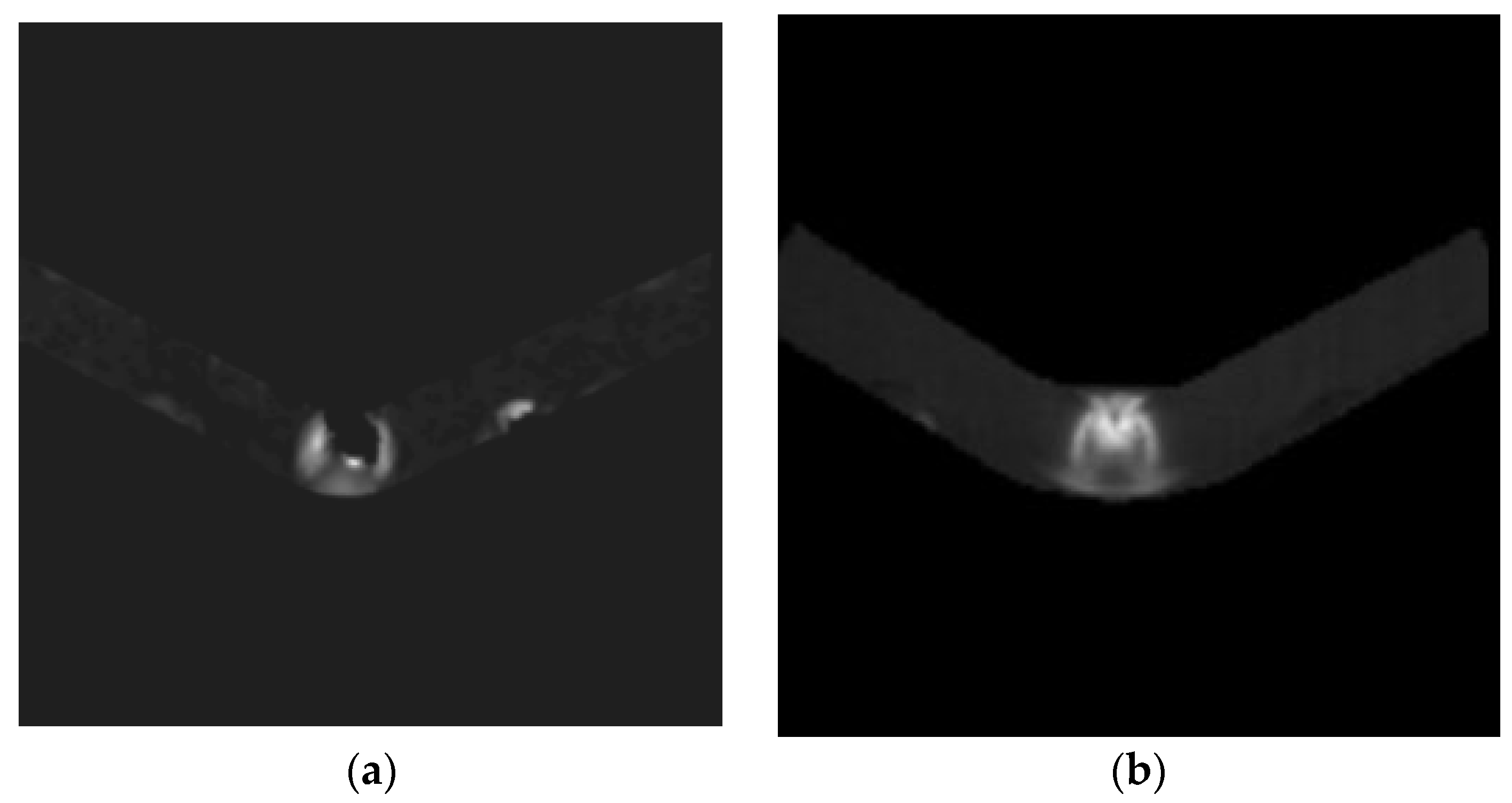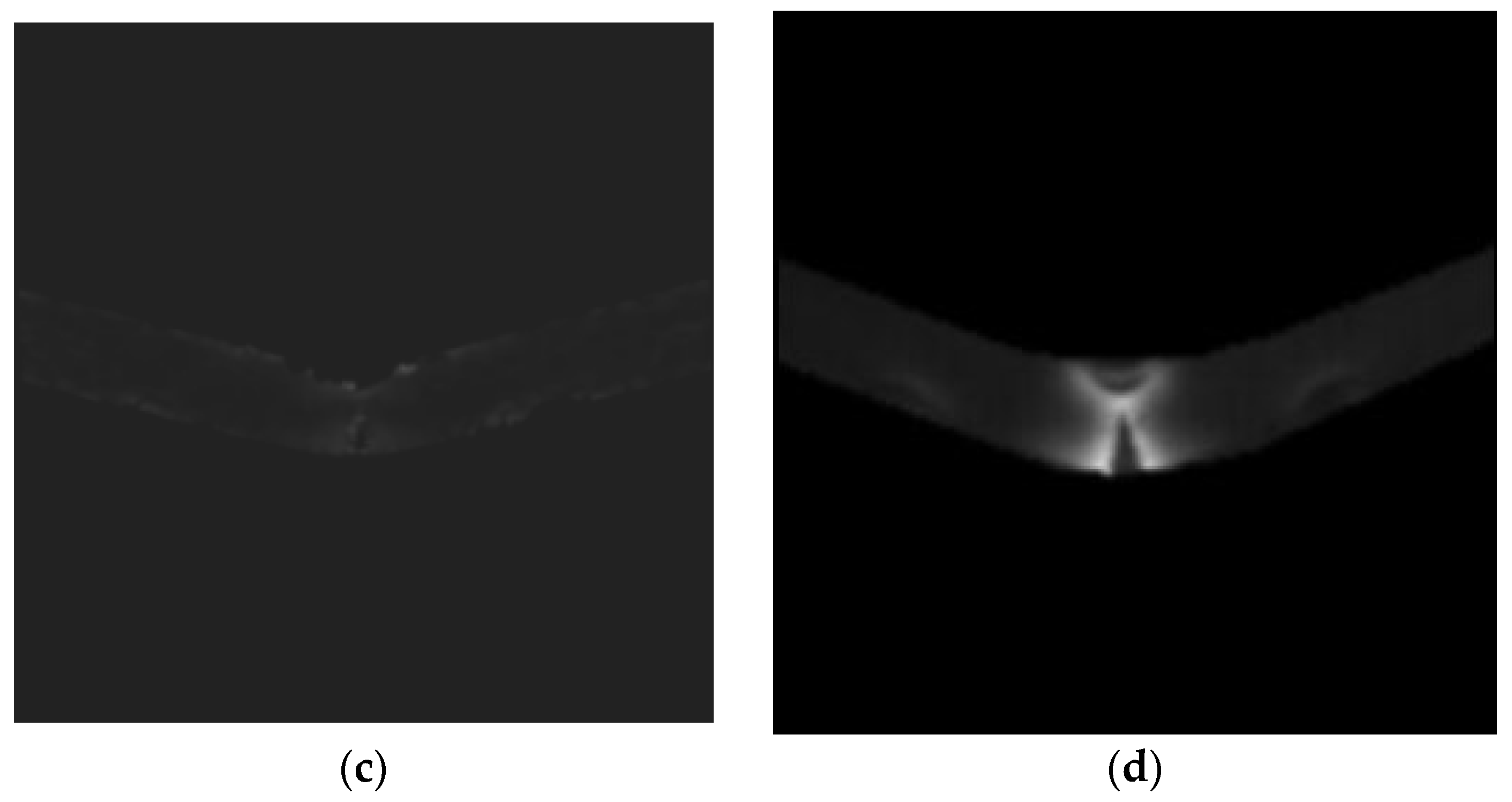Similar small-magnitude augmentations have been used in DIC accuracy studies to evaluate robustness to slight geometric perturbations [3,23], and this technique is also widely adopted in imaging tasks where dataset size is limited [24,25,26]. Each frame was augmented multiple times with random combinations of these transformations, expanding the dataset to from 189 to 1655 paired images. This increased variability helps reduce model overfitting and encourages the network to learn the true thermomechanical mapping instead of memorizing specimen-specific features. During dataset preparation, frames corresponding to the initial loading stages with negligible deformation were excluded, as both the strain and thermal fields in these frames contain very limited informative structure and could bias the learning process. This filtering step was applied prior to augmentation and was applied consistently across all subsets. After augmentation, the final dataset comprised 1655 paired images, with no overlap between training, validation, and test data. For consistency with the network input, both effective strain and temperature fields are shown in grayscale, exactly as they are provided to the deep learning model after normalization. While colour maps are commonly used for visualization, they were intentionally omitted here to emphasize the raw numerical field representation rather than qualitative colour perception. Paired effective strain and thermography images for two selected pairs are shown in Figure 5a,b and Figure 5c,d.

3. U-Net-Based Regression Architecture and Training Procedure

The goal of this part of the research was to learn a pixel-wise mapping from the effective strain field (obtained from DIC) to the corresponding temperature distribution measured by infrared thermography. For this purpose, a modified regression-based U-Net architecture was implemented.

3.1. Modifications to the Baseline U-Net Architecture

The classical U-Net introduced by Ronneberger et al. [7] was originally developed for biomedical image segmentation, where the network outputs are discrete pixel-wise class probabilities. MATLAB’s built-in U-Net layers follow this formulation and therefore terminate with a SoftMax [27] activation and a pixel-classification loss [7]. Since the goal of the present research is to predict a continuous-valued thermal field from strain images, the segmentation-oriented layer must be replaced with a regression formulation.

Default SoftmaxLayer and PixelClassificationLayer were removed and substituted with a single 1 × 1 convolution layer that produces one output regression channel corresponding to the predicted thermal intensity. This layer is directly connected to a regression output layer. Such conversion of U-Net from a classifier to a pixel-wise regressor is consistent with the broader literature, where U-Net and similar encoder–decoder architectures have been adapted to predict continuous physical fields, including stress distributions, thermal responses, or other spatially varying engineering quantities [28,29,30,31,32]. Recent studies demonstrate that this type of architecture performs well when learning mappings between engineering measurements or simulated fields. For example, Hoq et al. [28] employed a modified U-Net for regression of mechanical properties. U-Net-like models have also been applied for thermal response prediction in additive manufacturing [29], aerodynamic load estimation [31], and in more general physical-field regression tasks [30]. These works show that replacing the segmentation head with a regression head is a robust and widely used strategy for continuous field prediction in engineering applications. Representation of modified U-net architecture is derived from the original U-net architecture [7].

Except for the removal of the classification layers, the overall U-Net encoder–decoder structure was preserved. The skip connections, multi-scale feature extraction, and up-sampling layers remain unchanged, as these components help to maintain spatial accuracy while integrating global deformation context, which is critical for predicting temperature fields that arise from both localized strain increments and thermomechanical behaviour. The final architecture was implemented by modifying the layer graph produced by U-net layers, ensuring full compatibility with MATLAB’s deep learning workflow [33] (see Figure 6).

3.2. Training Procedure

The modified U-Net was trained to learn pixel-wise regression from normalized effective strain fields to their corresponding thermal maps. All input and target images were resized to 256 × 256 pixels, normalized to the range of 0–1, and prepared as paired datasets. The dataset was split into training (70%), validation (15%), and test (15%) subsets prior to augmentation. After preprocessing, a total of 1165 paired images were available for training. To establish a robust training configuration, five independent training runs were performed. Each run was trained for 400 epochs, allowing the optimization process to fully converge and enabling systematic comparison of loss functions and hyperparameters. Model validation was performed using a fixed hold-out strategy. The validation set was used for monitoring training convergence and selecting hyperparameters, while the test set was reserved for final performance evaluation.

During an early training session, it was established that for this dataset, convergence could be expected to be around 320 epochs. The Adam optimizer was used in all cases, due to its well-documented stability in deep learning applications involving continuous-valued regression [34]. Several loss formulations were investigated. In addition to the standard mean-squared error (MSE) loss, we evaluated L1 loss [35] and a weighted L1 loss [36]. The latter was designed to place additional emphasis on high-temperature regions where localized thermomechanical events occur. Despite this motivation, both L1-based losses resulted in inferior performance. Networks trained with L1 or weighted L1 tended to produce spatially noisier thermal fields and exhibited slower convergence. In contrast, the MSE-based training runs produced smoother predictions and more accurate reconstruction of hotspot regions. For this reason, the final model was trained using MSE loss. The reported validation MSE value of 2.3548 corresponds to the validation loss monitored during training and was computed as an image-wise average of pixel-level squared errors over validation batches. This value was obtained using a learning rate of 0.0001, which is commonly employed for stable CNN training with the Adam optimizer.

3.3. Inference, Evauation Metrics, and Accuracy Assesment

After training, 249 unseen test DIC frames were passed through the network to evaluate the accuracy of the temperature fields. The comparison between the DIC-derived effective strain, the predicted thermal images, and the corresponding ground-truth thermal images is shown in Figure 7.

Model performance was assessed on the reserved test set using several pixel-wise regression metrics. The root-mean-square error (RMSE) and mean absolute error (MAE) quantified the absolute difference between the predicted and measured temperature fields. The coefficient of determination (R²) [37] was computed across randomly sampled test images to evaluate overall agreement between predicted and true pixel intensities. In addition, the structural similarity index (SSIM) [38] was calculated to assess how well the network preserved spatial structure, contrast, and local correlations in the thermal field. Qualitative inspection—including side-by-side comparisons and residual maps—was also performed to verify that the network reproduced the main features of the thermographic response, particularly localized hotspots associated with deformation.

4. Results

The trained U-Net model demonstrated strong predictive performance on the test dataset. To quantitatively assess the generalization capability of the trained network, prediction accuracy was evaluated on an independent test dataset that was not used during training or validation.

Table 3. Performance metrics evaluated on the independent test dataset.

Metric	Test Set
SSIM	0.4262
MAE	0.0561
RMSE	0.0986
R2	0.968

summarizes the mean performance metrics computed on the test set, including SSIM, MAE, RMSE, and the coefficient of determination (R²).

4.1. Global Prediction Accuracy

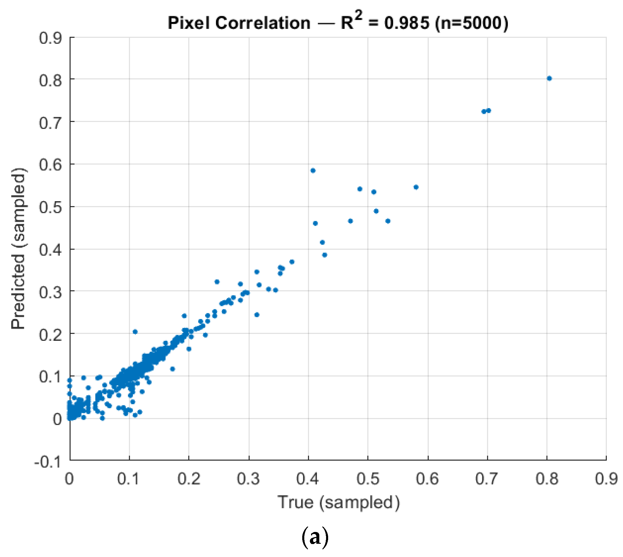
A global pixel-level comparison between predicted and true thermal fields (see Figure 7a) shows tight clustering around the identity line, indicating strong agreement between the predicted and measured temperatures.

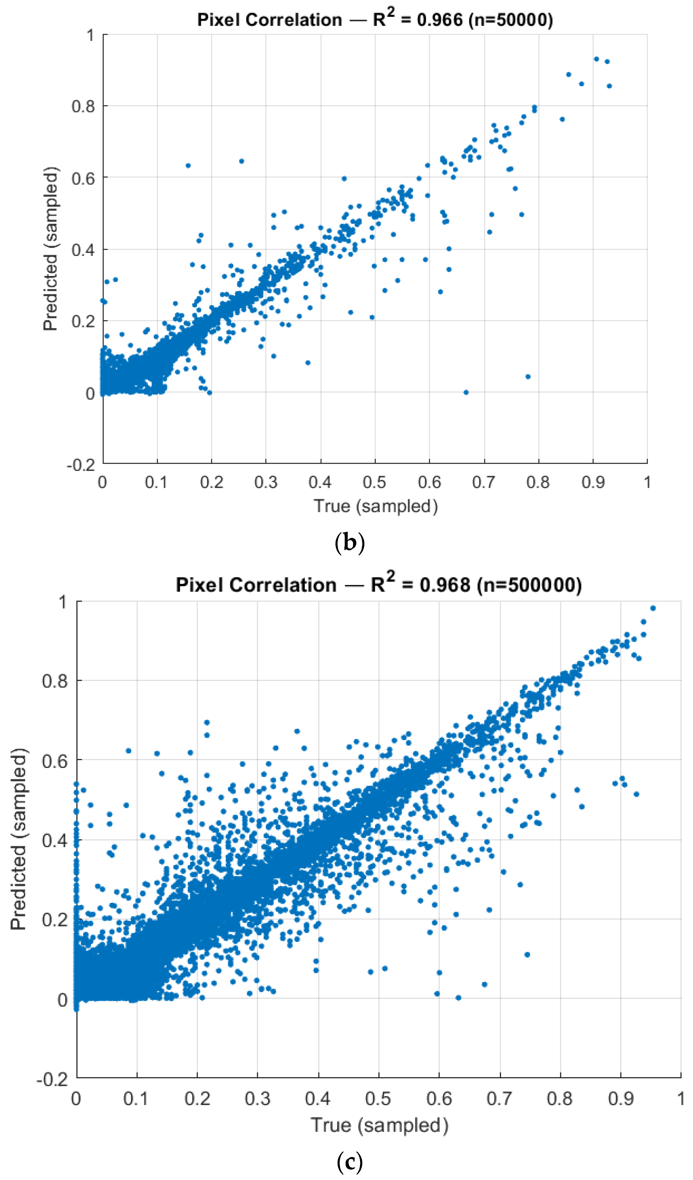
The coefficient of determination of R² = 0.985 was calculated on 5000 randomly sampled pixels from predicted and true thermal datasets. Additionally, 50,000 and 500,000 datapoints out of a possible 16,973,824 were sampled, with R² = 0.966 and R² = 0.968 respectfully (see Figure 8). This indicated that the learned mapping preserves the global distribution of thermal intensities with relatively high fidelity.

4.2. Spatial Distribution of Prediction Accuracy

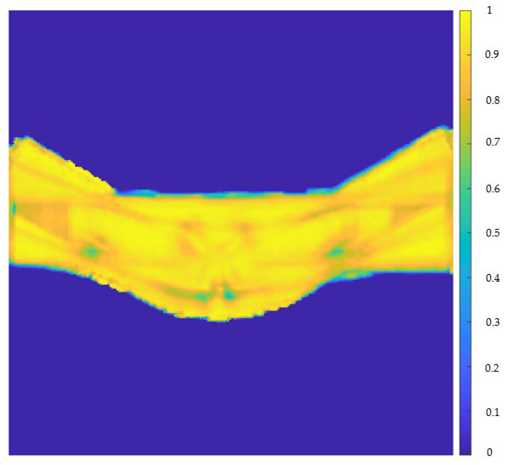
To further examine spatial consistency, a pixelwise R² field was computed across the entire image domain (see Figure 9).

The central region corresponding to the deforming specimen exhibits uniformly high agreement (R² ≈ 0.8–1.0), while the background and masked regions show lower values, as expected, due to near-zero temperature gradients that amplify relative errors. The predicted thermal fields obtained from the trained U-Net remained largely within this physically meaningful range, with values spanning from −0.0615 to 0.9825. The small drift into negative values (≈6% below zero) is expected for convolutional regression networks trained without an explicit output constraint or activation function at the final layer. Such networks can produce unbounded continuous outputs, and slight under- or overshooting near sharp gradients or data-sparse regions is common. These deviations are minor relative to the dynamic range of the normalized data and do not introduce structural artifacts. In practice, negative predictions can be safely clamped to zero during inference without loss of information, while the upper range remains relatively aligned with the true values.

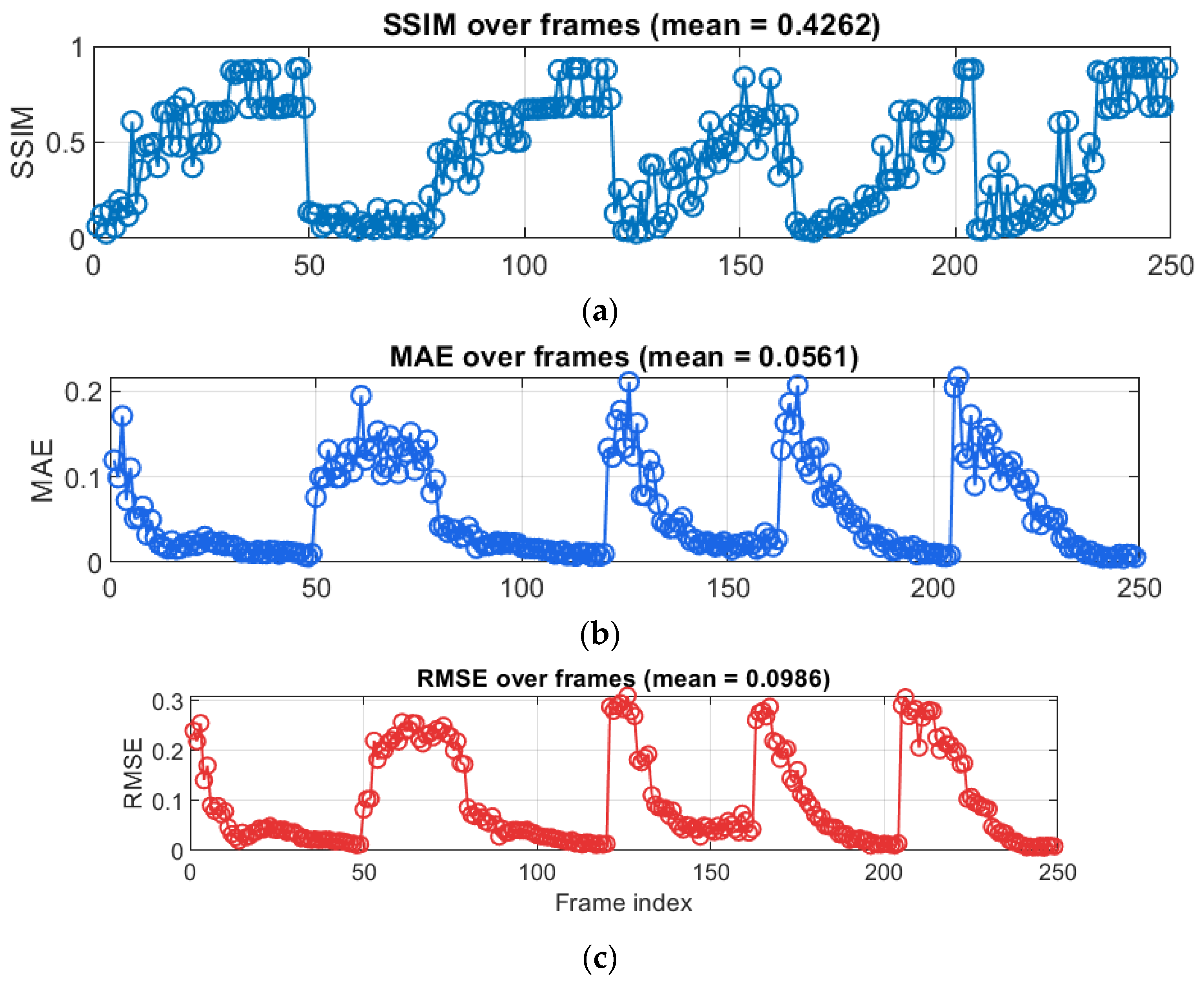
Error distributions over the test dataset were quantified using SSIM, MAE, and RMSE (Figure 10). A clear and physically meaningful trend is observable: the prediction error is largest in the earliest test frames, when the specimen is still undeformed and the thermal field contains very low spatial variation. In this initial stage, the true thermal images are dominated by nearly uniform background with minimal temperature gradients.

4.3. Frame-Wise Error Evolution

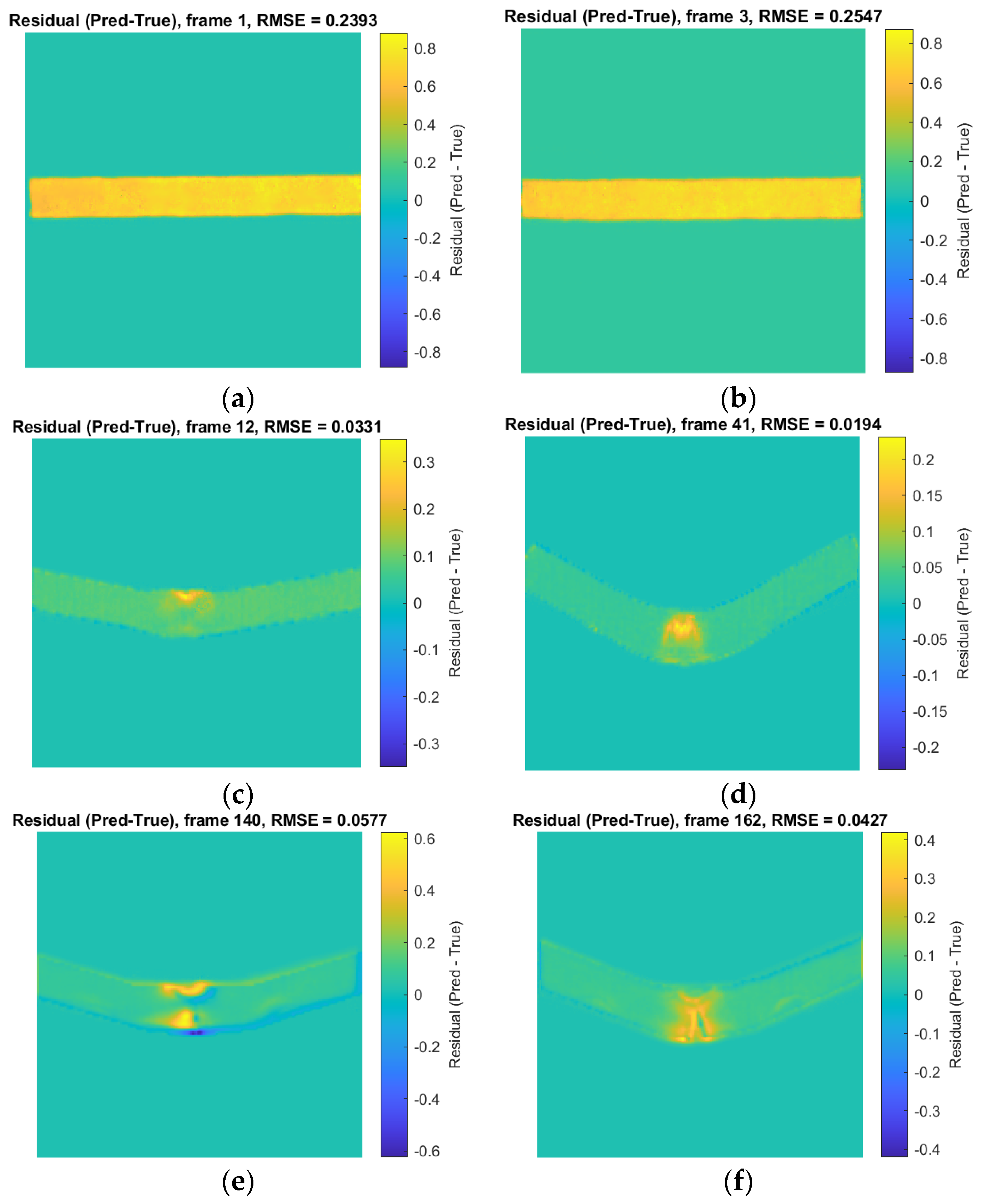
Because the strain fields at this point also contain only noise-level deformation, the mapping between DIC strain and thermal response is weakly defined, and small pixel-level deviations lead to comparatively high normalized error (e.g., RMSE ≈ 0.24–0.26 in frames 1 to 3, see Figure 11). The residual maps for these frames confirm that the network slightly overpredicts a uniform heating pattern along the specimen. As loading begins and deformation localizes, the thermal field becomes more characteristic and structured. Correspondingly, the network’s performance improves significantly. Between approximately frames 6 and 50 (see Figure 10), the MAE stabilizes around 0.02–0.04, the RMSE falls to 0.01–0.03, and the SSIM reaches 0.6–0.8, indicating very good agreement. Representative residual maps (e.g., frames 12 and 41, see Figure 11) show that discrepancies are confined to small areas around the forming “hinge”, where temperature gradients are steepest. As the test progresses into the large-rotation region (frames 140–162, see Figure 11), prediction quality remains strong despite increasing geometric complexity RMSE ≈ 0.05 and SSIM ≈ 0.5.

Overall, the error curves demonstrate that the U-Net model is most accurate during the mechanically meaningful phases of the experiment, where the thermomechanical coupling between strain and temperature is strongest. Importantly, no systematic artifacts or hallucinations appear in any residual map, and all deviations from true data remain physically interpretable. The largest errors are observed in frames with little or no informative thermal structure (i.e., initial uniform states where deformations are practically noise) and a few post-peak frames. Generally, the model attains low error and high structural similarity during the main deformation phase, where thermomechanical interpretation is most critical. The final trained U-Net model is relatively compact by modern deep learning standards, with approximately 31.0 million learnable parameters and a disk size of ≈110 MB. This moderate model capacity was sufficient to capture the thermomechanical mapping while remaining computationally efficient for both training and inference.

5. Discussion

The results indicate that the learned effective strain-to-temperature mapping follows the general thermomechanical behaviour observed in previous experimental studies, where temperature localisation coincided with the onset of plastic deformation and strain concentration [6,10]. In the present work, this relationship is clearly reflected in the frame-wise error evaluation. The highest prediction errors occur in the initial part of the loading sequence, where both the strain field and the thermal response exhibit very limited spatial structure. In these nearly uniform states, even small absolute deviations can translate into comparatively large, normalized errors, and similarity measures such as SSIM remain low.

As deformation progresses, the model accuracy improves substantially. Once measurable strain localization develops, the network predicts temperature fields with low RMSE and markedly higher structural similarity. The residual maps confirm that, in this regime, most discrepancies remain confined to narrow regions where gradients change sharply or where local decorrelation effects in the DIC data introduce noise. This behaviour is consistent with the expectation that prediction quality increases when the thermomechanical signal becomes stronger and more informative.

These observations suggest that data-driven thermal reconstruction is most reliable during the mechanically relevant stages of loading, where temperature gradients are typically analyzed for damage initiation or energy dissipation. While the reduced fidelity observed in the early, nearly uniform frames is of limited practical significance, it should be taken into consideration in future retraining strategies. Overall, the model reconstructs the thermal field without introducing non-physical artefacts and preserves the essential spatial structure of the thermographic response. The comparable temperature and effective strain ranges observed across the datasets (Table 2) further suggest that the trained model may be transferable to experiments characterized by similar thermomechanical operating regimes and materials with comparable properties.

The present study is intended as a proof of concept demonstrating that full-field temperature distributions can be reconstructed directly from strain measurements using a data-driven deep learning framework. To this end, specimens with relatively symmetric geometries subjected to three-point bending were deliberately selected, as this configuration provides a predictable deformation pattern and a well-defined thermomechanical response, enabling controlled validation of the proposed approach.

As a consequence, the current experimental dataset does not include strongly asymmetric geometries, complex boundary conditions, or a broader range of material classes. While the proposed framework itself is not inherently limited to symmetric parts or a specific material, its performance under such conditions has not yet been experimentally verified. Future work will therefore focus on extending the framework to different materials, asymmetric geometries, and alternative loading scenarios, as well as expanding the dataset to assess generalization capability and robustness under more complex thermomechanical conditions.

In addition to experimental extensions, further research directions include the investigation of shared-encoder architectures, in which a single feature extractor feeds separate mechanical and thermal decoders. Such designs may reduce redundancy and strengthen the coupling learned between the two fields. It would also be valuable to retrain image-to-image translation models such as pix2pix on the same dataset to directly compare adversarial and regression-based approaches, particularly in their ability to capture fine thermal details or handle low-information strain inputs. Finally, incorporating temporal models, such as recurrent or attention-based architectures, could exploit frame-to-frame continuity and further improve prediction stability during high-rate deformation.