Super-Twisting Algorithm Sliding Mode Control of Flexible Manipulators Considering Uncertainty

Abstract

The dynamic model of a spatial flexible manipulator is challenging to establish accurately and is susceptible to disturbances from uncertainties, which negatively impact system control. To mitigate the effects of uncertainties and improve control precision, this paper develops the dynamic model of a spatial flexible manipulator system using the Lagrange principle and the assumed mode method. Additionally, to address the chattering issue in sliding mode control, a super-twisting algorithm sliding mode control strategy is proposed, which utilizes an RBF neural network to compensate for system uncertainties. By incorporating the concept of higher-order sliding mode, the super-twisting algorithm sliding mode is integrated with non-singular terminal sliding mode to design the sliding surface and control law, ensuring the stable and rapid convergence of the system state while reducing chattering. The simulation results demonstrate that the proposed strategy reduces fluctuations in rotation angle and angular velocity errors at both the input and output ends, enhances trajectory tracking performance, and achieves effective chattering suppression.

1. Introduction

In the field of space robotics, flexible manipulators have garnered significant attention due to their distinctive advantages. Compared to traditional industrial manipulators, which are characterized by high rigidity, high energy consumption, and relatively low precision, flexible manipulators feature lightweight long-link structures, low moment of inertia, and high transmission efficiency [1]. These attributes make them well-suited for applications in space exploration. A spatial flexible manipulator constitutes a complex high-order, strongly coupled, nonlinear, and time-varying system. It faces challenges such as vibrations induced by structural flexibility, model uncertainties, parameter variations, and external disturbances. If not properly controlled, these issues may degrade system performance and stability.

In the work by Shang D et al. [2], the dual-flexibility coupling and two-dimensional deformation characteristics of the system are explored. This paper employs the assumed mode method to describe the transverse and longitudinal deformations of the flexible load and establishes a dynamic model using Lagrange’s theorem. Furthermore, the vibration mechanism of the flexible manipulator is explained from an energy perspective, providing valuable insights for system modeling in this field.

Numerous control strategies have been developed to address system uncertainties and parameter variations in the control of spatial flexible manipulators. These include fuzzy algorithms [3], PID control [4], reinforcement learning [5], singular perturbation methods [6], and sliding mode control [7]. As an important branch of variable structure control, SMC is well-known for its insensitivity to system uncertainties and parameter variations [8]. Consequently, it has been widely applied in satellite systems [9], robotic manipulators [10], and other fields. However, conventional SMC suffers from issues such as slow response, singularities, and chattering in the control input [11]. To overcome these limitations, a non-singular terminal sliding mode (NTSM) approach was designed in and applied to multi-joint manipulator systems, enabling stable and rapid convergence to the equilibrium point. Despite this improvement, NTSM still exhibits chattering, which degrades system performance. To suppress chattering, Reference [12] replaced the sign function with a hyperbolic tangent function, while Van M et al. [13] designed the sliding surface using a saturation function. In contrast, Zhang J et al. [14] employed a higher-order sliding mode (HOSM) to design the control law. By increasing the sliding order to hide discontinuities, this approach effectively reduces chattering while maintaining the strong robustness of first-order SMC. Nevertheless, it sacrifices robustness within the boundary layer of the switching function to achieve smoothness. To address these trade-offs, a super-twisting algorithm sliding mode control was proposed in [15]. This method preserves the advantages of HOSM and introduces an integral term to compensate for disturbances and smooth the output. Its structure inherently avoids high-frequency switching, thereby significantly mitigating chattering.

On the other hand, the motion of flexible joints is significantly affected by nonlinear friction torque [16]. Therefore, nonlinear friction models must be considered when establishing the dynamic equations of spatial flexible manipulator systems. Additionally, as the system itself contains numerous nonlinearities, researchers often treat external disturbances (such as nonlinear friction) and other nonlinear terms as system uncertainties [17]. Substantial uncertainties in the model can induce chattering. This phenomenon can cause severe damage to actuators and mechanical components, making adequate compensation for model uncertainties particularly necessary. For instance, Reference [18] employed a disturbance observer to asymptotically estimate unmodeled external disturbances and compensate for their effects. Consequently, the integration of disturbance observers with sliding mode control to suppress chattering from the perspective of external disturbances has become a research focus in the SMC field [19]. With advancements in intelligent control, neural network techniques have also been widely adopted in robotics control. The Radial Basis Function (RBF) neural network, leveraging its universal approximation capability, can accurately approximate nonlinear dynamic parameters through an online learning mechanism [20]. In Reference [21], an RBF neural network was utilized to identify and compensate for uncertainties in a flexible manipulator system. By designing adaptive and control laws, the adverse effects of friction torque and nonlinearities were effectively mitigated.

To address the aforementioned challenges in spatial flexible manipulators, we develop the system dynamics using Lagrange’s theorem and the assumed mode method. A super-twisting algorithm sliding mode control strategy, enhanced by a Radial Basis Function (RBF) neural network, is designed to compensate for system uncertainties. This integrated approach mitigates chattering induced by unmodeled dynamics and other uncertainties from multiple perspectives. The effectiveness of the proposed control strategy is validated through simulation experiments.

Regarding dynamic modeling, this work adopts the established Lagrangian method and assumed mode approach. This model accurately describes the dynamics of a dual-flexible servo system incorporating two-dimensional deformation, friction, and time-varying length, and its validity for precise representation has been previously verified. The primary contribution of this work lies in the control strategy. We propose a distinct improvement to address the chattering issue inherent in conventional sliding mode control (SMC) for flexible manipulators. While existing methods often mitigate chattering by modifying the switching function or introducing a boundary layer, our approach diverges by employing higher-order sliding mode (HOSM) concepts [14]. Specifically, the super-twisting algorithm (STA)—an HOSM method—is applied to the flexible manipulator servo system. The super-twisting algorithm sliding mode control (STASMC) inherently suppresses chattering structurally while maintaining robustness against parameter variations and uncertainties. Furthermore, this is coupled with an RBF neural network that provides the real-time approximation of the system’s nonlinear and time-varying components. Together, they form a dual-enhancement mechanism characterized by “high-order chattering suppression + uncertainty compensation”. The proposed method theoretically guarantees finite-time convergence and enhanced stability, with its effectiveness being validated through simulation experiments.

2. Problem Representation and Dynamic Model Establishment

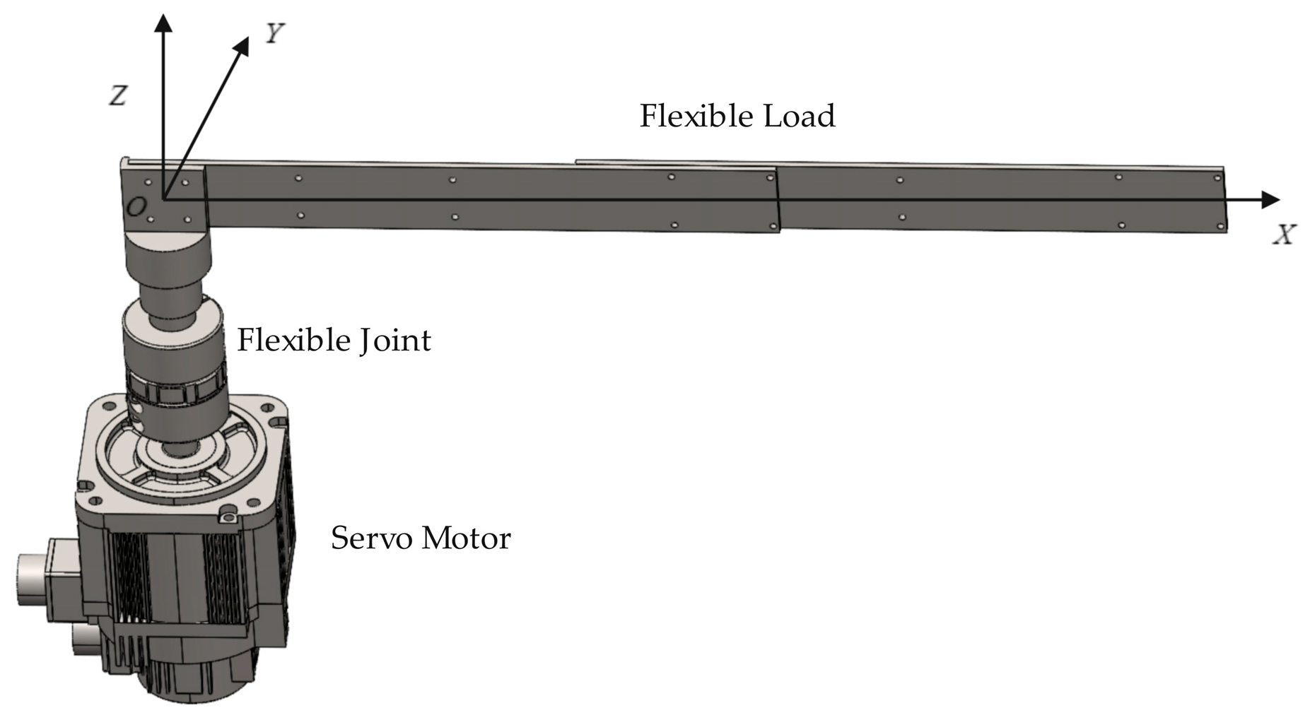
Throughout this paper, the terms “flexible manipulator” and “flexible load” refer to distinct but related concepts within the studied servo system. The flexible manipulator denotes the entire mechanical structure, which comprises a servo motor, a flexible joint, and a driven link that exhibits significant compliance. The flexible load specifically refers to that compliant driven link (modeled as a Euler–Bernoulli beam model) which is connected to the motor via the flexible joint and undergoes two-dimensional deformation during operation. Thus, the flexible load is a key component of the flexible manipulator system, and its dynamics are the primary focus of the modeling and control design presented in this work.

In view of the research status in the field of space robot, its mainstream control strategy focuses on joint control and whole arm control based on a dynamic model [22]. For the convenience of assumption and research, we model the entire system as a single-link manipulator, actuated by a motor through flexible joints, as shown in Figure 1. In line with many established studies in this field, this work simplifies the spatial flexible manipulator system to a planar single-link model for investigation. The core dynamic challenge of the spatial manipulator—namely, the coupling between vibrations induced by flexible deformation and the rotational motion—is fully preserved in this simplified model. Secondary factors, such as three-dimensional spatial rotations, would significantly increase the complexity of the equations. This model therefore focuses effectively on the essential dynamics, thereby reducing the complexity of both modeling and control design.

The effective description of flexible load deformation is the key link, and the assumed mode method is a widely used and effective method in this field [23]. Based on Assumption 2, we regard the flexible load as a Euler–Bernoulli beam model [24], and use the assumed mode method to characterize the elastic deformation of the flexible load. In order to simplify the above discussion before the establishment of the dynamic model, the following basic assumptions are introduced:

Assumption 1.

Only the fixed-axis rotation of the flexible load in the XOY plane is considered.

Assumption 2.

In view of the fact that the flexible load bar is far longer than its cross-sectional size, it is regarded as a slender beam.

Assumption 3.

In the space environment, the influence of the gravity of the flexible load itself is ignored.

Assumption 4.

The deformation of the flexible payload satisfies the conditions of inextensibility along the neutral axis and small deformations.

Based on the above assumptions and modeling method, the lateral deformation of the flexible load can be described as

$$w(x,t)=\varphi (x)\eta (t)={\displaystyle \sum _{i=1}^{\infty }{\varphi }_i}(x){\eta }_i(t)$$

(1)

where ${\varphi }_i(x)$ is the i-th order modal function and ${\eta }_i(t)$ is the corresponding modal coordinate. Based on Assumption 4, the relationship between transverse deformation $w\left(x,t\right)$ and longitudinal deformation $u\left(x,t\right)$ can be expressed as

$$u(x,t)=-{\displaystyle \frac{1}{2}}{\displaystyle {\int }_0^x(\frac{\omega (\mathsf{\sigma },t)}{\partial \mathsf{\sigma }}}{)}^{2}d\mathsf{\sigma }$$

(2)

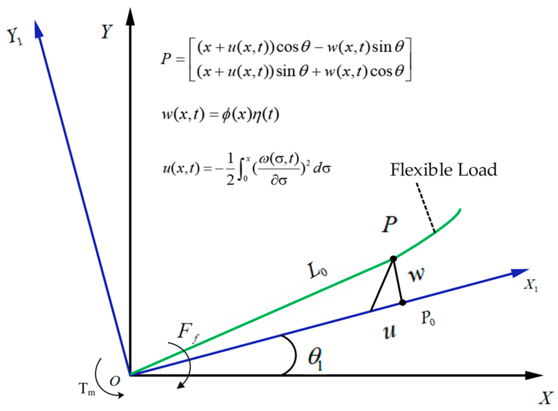
In order to further intuitively characterize the spatial flexible manipulator system considering both lateral and longitudinal deformation of the load, the static coordinate system O-XYZ fixed to the ground and the rotating coordinate system O-X₁Y₁Z₁ during the movement are established in Figure 2. The Z₁ axis (rotation axis) coincides with the Z axis (rotation center of the manipulator), in which the motion of the flexible load can be decomposed into elastic deformation caused by the traction motion of the rotating coordinate system and rigid body motion relative to the rotating coordinate system.

The length of the flexible load is $L_0$, Tm is the input torque of the servo motor, $F_f$ is the friction and ${\theta }_{\mathrm{l}}$ denotes the rotation angle of the flexible load. During motion, an arbitrary point $P_0$ on the undeformed flexible link moves to position $P$ after deformation, as illustrated in Figure 2, and the P position of any point on the flexible load can be expressed as

$$P=\left[\begin{array}{c}(x+u(x,t))\cos \theta -w(x,t)\sin \theta \\ (x+u(x,t))\sin \theta +w(x,t)\cos \theta \end{array}\right]$$

(3)

The total kinetic energy of the system is composed of the kinetic energy of the load end and the kinetic energy of the motor end, as shown in the following equation:

$$T={\displaystyle \frac{1}{2}}\rho A{\displaystyle {\int }_0^{L_0}{(\dot{P})}^{2}dx+\frac{1}{2}{J}_m{(\dot{\theta })}^2}$$

(4)

In the formula, $\rho A$ is the linear density of the flexible load, and $J_m$ is the moment of inertia of the motor. The space environment does not consider the gravitational potential energy. The potential energy of the system is composed of the elastic potential energy of the flexible load and the elastic potential energy of the flexible joint.

$$V={\displaystyle \frac{1}{2}}{K}_s{({\theta }_l-{\theta }_m)}^2+{\displaystyle \frac{1}{2}}EI{\displaystyle {\int }_0^{L_0}{(w^{″})}^2}dx$$

(5)

where $K_s$ is the torsional stiffness coefficient of the joint, $E$ denotes the elastic modulus, $I$ represents the area moment of inertia of the cross-section, and ${\theta }_{\mathrm{l}}$ denotes the rotation angle of the flexible load, while ${\theta }_{\mathrm{m}}$ represents the rotation angle at the motor end. Part of the vibration mechanism of the system can be explained by the formula. Due to the existence of its own structural flexibility, the spatial flexible manipulator will store elastic potential energy during its movement. When the potential energy is released, it can cause system vibration.

The Lagrange function is introduced by the Lagrange second principle combined with the vibration theory. The dynamic equation of the spatial flexible manipulator system can be established as follows:

$${\displaystyle \frac{d}{dt}}\left({\displaystyle \frac{\partial T}{\partial {\dot{q}}_j}}\right)-{\displaystyle \frac{\partial T}{\partial q_j}}+{\displaystyle \frac{\partial V}{\partial q_j}}=Q_j$$

(6)

The generalized coordinate vector $q={[{\theta }_m,{\theta }_l,\eta ]}^T$ and generalized force vector $Q={[T_m,0,0]}^T$ are defined to describe the system motion.

Considering the dynamic characteristics of the system, the LuGre [25] model with more comprehensive friction characteristics is selected to characterize the friction nonlinear term in the transmission system:

$$\left.\begin{array}{c}{F}_f={\sigma }_{0}z+{\sigma }_1\dot{z}+{\sigma }_2{\dot{\theta }}_m\\ \dot{z}={\dot{\theta }}_m-{\sigma }_0{\displaystyle \frac{\left|{\dot{\theta }}_m\right|}{g({\dot{\theta }}_m)z}}\\ g({\dot{\theta }}_m)=M_c+(M_s-M_c)\exp (-{\left|{\displaystyle \frac{{\dot{\theta }}_m}{{\theta }_s}}\right|}^2)\end{array}\right\}$$

(7)

Among them, $z$ is the average friction deformation, ${\sigma }_0$ is the friction stiffness coefficient, ${\sigma }_1$ is the friction damping coefficient, ${\sigma }_2$ is the viscous friction coefficient, $g\left({\dot{\theta }}_m\right)$ is a nonlinear function describing the Stribeck effect, which is asymmetric and always greater than 0, ${\theta }_s$ is the friction velocity coefficient, $M_{\mathrm{c}}$ is the coulomb friction torque, and $M_s$ is the static friction torque.

The choice of modal coordinate order during system modeling directly influences both the model’s accuracy and computational efficiency. Theoretically, retaining higher-order modes can more accurately approximate the dynamic characteristics of a continuous system, but it significantly increases control system complexity and computational burden. Research [26] indicates that the dynamic response of a flexible manipulator is predominantly governed by its first-order mode, whose contribution substantially exceeds the combined effects of all higher-order modes. Furthermore, the deformation deviation between the two-dimensional deformation of the flexible load and the neglected nonlinear coupling terms is negligible. The study indicates that the first-order natural frequency of the flexible load (10–20 Hz) is significantly higher than the system’s dominant rotational motion frequency (0.1–0.3 Hz), demonstrating a clear frequency separation. As the natural frequencies of higher-order modes are even higher, their excitation energy during the system’s low-frequency motion is extremely limited. Furthermore, numerical analysis shows that under the given operating condition, the maximum amplitude of transverse deformation is on the order of 10⁻², while the longitudinal deformation amplitude is only on the order of 10⁻⁵. This verifies that neglecting higher-order modes, nonlinear coupling terms, and longitudinal deformation does not significantly affect model accuracy. Therefore, retaining only the first-order mode is well-justified for dynamic analysis and control strategy design. Following this conclusion, this work retains the first-order mode while neglecting the coupling nonlinear terms. Integrated with the LuGre friction model, the dynamic equations of the spatial flexible manipulator system are derived as follows:

$$M(q)\ddot{q}+K(q)q+F(q,\dot{q},\ddot{q})=u$$

(8)

In the formula, $M(q)$ is the inertia matrix, $K(q)$ is the stiffness matrix, $F(q,\dot{q},\ddot{q})$ is the disturbance term, $u$ is the control input of the system. The specific parameters of the above formula are shown in the Appendix A. In this paper, the LuGre friction model is primarily used to construct a high-fidelity simulation benchmark, accurately reflecting the complex friction characteristics of a real system. In terms of controller design, however, this friction is treated as a bounded nonlinear disturbance. It is compensated for online by the RBF neural network, thereby enhancing the robustness of the controller.

3. Super-Twisting Sliding Mode Control Based on Neural Network Compensation

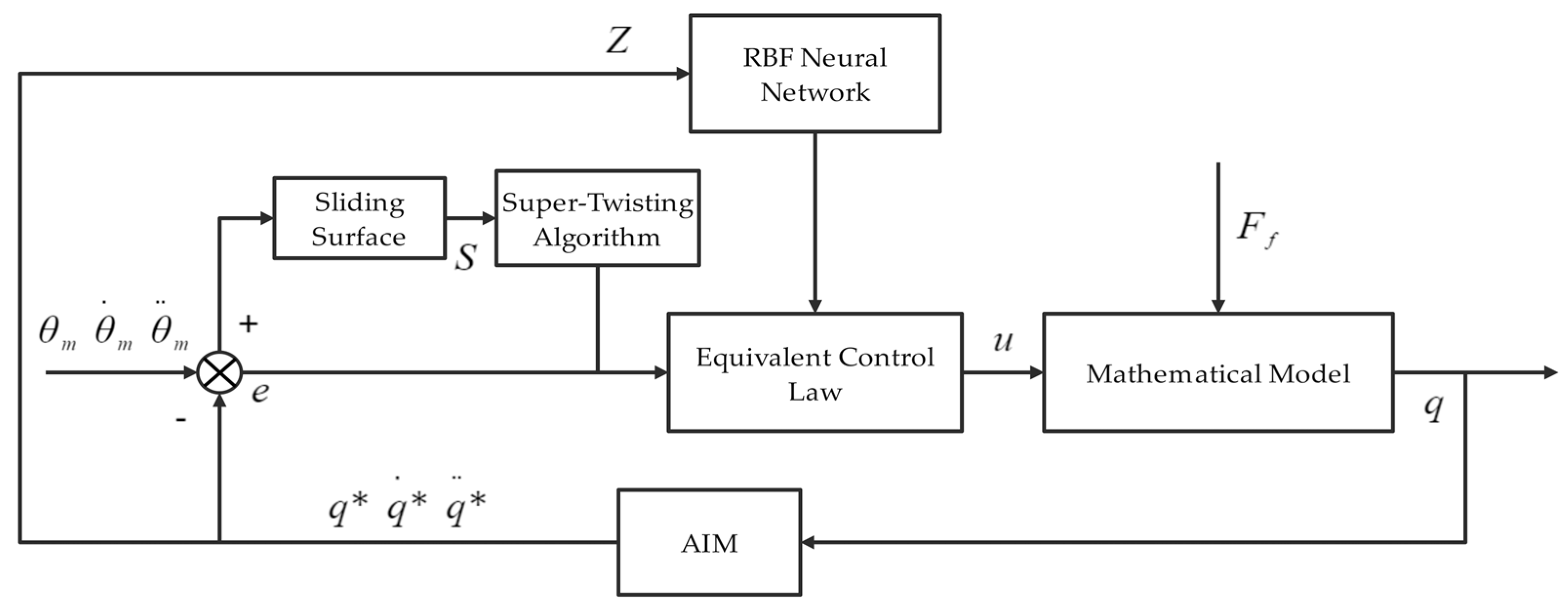
Based on the system model of the spatial flexible manipulator, the control block diagram is shown in Figure 3. As regards the system chattering problem, it is worth noting that it is mainly caused by unmodeled uncertain components, and the state of the switching function is also an important factor. In order to solve this problem, on the one hand, we use the RBF neural network to identify and compensate for the uncertain components. On the other hand, we design a super-twisting algorithm sliding mode control strategy, which is insensitive to the uncertain components of the system, and introduces the integral term from the structure to avoid high-frequency switching and suppress system chattering from multiple angles. AIM is a commonly used method in this field for obtaining the desired input [26].

3.1. Super-Twisting Algorithm Sliding Mode Design

Super-twisting algorithm sliding mode control is a second-order sliding mode control technology that can be used when the relative order of the system is one. By introducing an integral link, the chattering problem of traditional sliding mode control is effectively eliminated. The core idea is to transfer the discontinuous control term to the derivative of the control input.

The expected generalized displacement vector is defined, and the tracking error and derivative are defined as

$$\left.\begin{array}{l}e=q^{*}-q\\ \dot{e}={\dot{q}}^{*}-\dot{q}\\ \ddot{\mathrm{e}}={\ddot{q}}^{*}-\ddot{q}\end{array}\right\}$$

(9)

Here, $e$ denotes the tracking error vector, $q*={[{\theta }_{\mathrm{m}}*,{\theta }_l*,\eta *]}^T$ denotes the generalized displacement vector, and ${\dot{q}}^{*}$ and ${\ddot{q}}^{*}$ are the first derivative and the second derivative of the expected generalized displacement vector. The design of the sliding surface in the sliding mode controller usually takes the linear form $\mathrm{s}=\dot{e}+\lambda \mathrm{e}$, and the convergence speed will decrease significantly when the error is close to zero. In order to ensure that the tracking error converges in a finite time after reaching the sliding surface and enhance the dynamic performance of the system, the sliding surface is designed in accordance with the idea of nonsingular terminal sliding mode:

$$s=\dot{e}+\lambda | e {|}^{\alpha -1}\mathrm{sgn}(e)$$

(10)

Among these, $\lambda =diag\left({\lambda }_1,{\lambda }_2,{\lambda }_3\right)>0$ is a positive definite diagonal matrix, where $\alpha \in \left(1,2\right)$ is the estimated weight, set as such to ensure that the system state converges to the equilibrium point in a finite time, and when it does so, that it will not produce a singularity, so as to avoid the development of the terminal sliding mode near the origin of the control divergence problem. For the subsequent design of the equivalent control law, the derivative of the sliding surface is

$$\begin{array}{c}\begin{array}{cc}M\dot{s}& = M({\ddot{q}}^{*}-\ddot{q}+\lambda (\alpha -1) | e {|}^{\alpha -2} \dot{e})\hfill \\ & = M({\ddot{q}}^{*}+\lambda (\alpha -1) | e {|}^{\alpha -2} \dot{e})-M\ddot{q}\hfill \\ & = M({\ddot{q}}^{*}+\lambda (\alpha -1) | e {|}^{\alpha -2} \dot{e})+Kq+F-u\hfill \\ & = -u+f(z)\hfill \end{array}\end{array}$$

(11)

The control input $u$ can be observed in the expression of $\dot{\mathrm{s}}$. Therefore, the relative degree of the system with respect to the sliding variable $\mathrm{s}$ is one. This satisfies the application conditions for the super-twisting algorithm. The uncertain component can be expressed in the form of the following equation:

$$f(z)=M({\ddot{q}}^{*}+\lambda (\alpha -1) | e {|}^{\alpha -2} \dot{e})+Kq+F$$

(12)

3.2. Neural Network Design

In practical engineering, the uncertainty of the model is unknown, so it is necessary to approximate the uncertainty. The RBF neural network has a simple network structure and a good generalization ability. It can approximate any nonlinear function with any precision. The input of the RBF network is designed as follows:

$$z=\left[\begin{array}{c}{e}^T,{\dot{e}}^T,q^{*T},{\dot{q}}^{*T},{\ddot{q}}^{*T}\end{array}\right]$$

(13)

In the network algorithm, the Gaussian function is set as the hidden layer activation function,

$$h_j(z)=\exp (-{\displaystyle \frac{{‖z-c_j‖}^2}{2b^2}}),\hspace{1em}j=1,2,\dots ,7$$

(14)

Here, $c_j$ is the network center, $b$ is the width parameter, and the network output is

$$\widehat{f}(z)={\widehat{W}}^{T}h(z)$$

(15)

Among them, $\widehat{W}$ is an online updated weight matrix, and its priori is unknown. It is very important to design an adaptive control rate estimation approach. The weight adaptive law is designed as

$$\dot{\widehat{W}}=\mathsf{\Gamma }h(z)s^T$$

(16)

Thus, we obtain the following equation:

$$\dot{\tilde{W}}=-\mathsf{\Gamma }h(z)s^T$$

(17)

Here, $\mathsf{\Gamma }>0$ is the learning law matrix. The super-twisting algorithm sliding mode control law is designed using the following equation:

$$\left.\begin{array}{l}u=\widehat{f}(z)+k_1 | s {|}^{\alpha -1}\mathrm{sgn}(s)-v\\ \dot{v}=-k_2\mathrm{sgn}(s)\end{array}\right\}$$

(18)

The design control parameters are $k_1,k_2>0$. The core feature of the super-twisting algorithm lies in its incorporation of an integral term. This is realized through an auxiliary state variable, which makes the integral action continuous and pushes the discontinuous control to the derivative layer. As a result, the algorithm theoretically suppresses the high-frequency chattering inherent in conventional sliding mode control.

3.3. Stability Analysis

To establish the mathematical rigor of the proposed RBF neural network-based super-twisting algorithm sliding mode control strategy, a stability analysis is performed. Consider the Lyapunov candidate function, defined as

$$L={\displaystyle \frac{1}{2}}{s}^{T}Ms+{\displaystyle \frac{1}{2}}{v}^{T}v+{\displaystyle \frac{1}{2}}\mathrm{tr}({\tilde{W}}^T{\mathsf{\Gamma }}^{-1}\tilde{W})$$

(19)

Assuming that $W*$, an ideal weight, exists, the weight estimation error is designed as

$$\tilde{W}=W^{*}-\widehat{W}$$

(20)

Thus, we derive

$$f(z)=W^{*T}h(z)+ϵ$$

(21)

where $ϵ$ is the approximation error and $‖ϵ‖\le {ϵ}_N$ is assumed to be bounded. Then, Formula (12) can be expressed as

$$\begin{array}{cc}M\dot{s}& =-u+f(z)\hfill \\ & = f(z)-\widehat{f}(z)-(k_1 | s {|}^{\alpha -1}\mathrm{sgn}(s)-v)\hfill \\ & = \tilde{f}(z)-(k_1 | s {|}^{\alpha -1}\mathrm{sgn}(s)-v)\hfill \\ & = \tilde{f}(z)-\tau \hfill \end{array}$$

(22)

Among these,

$$\tilde{f}(z)=f(z)-\widehat{f}(z)$$

(23)

$$\tau =k_1|s{|}^{\alpha -1}\mathrm{sgn}(s)+v$$

(24)

The derivation of the Lyapunov candidate function involves

$$\begin{array}{c}\begin{array}{l}\dot{L}=s^{T}M\dot{s}+{\displaystyle \frac{1}{2}}{s}^T\dot{M}s+tr\left({\tilde{W}}^T{\mathsf{\Gamma }}^{-1}\dot{\tilde{W}}\right)+v^T\dot{v}\\ =s^T(\tilde{f}(z)-\tau )+{\displaystyle \frac{1}{2}}{s}^T\dot{M}s+tr\left({\tilde{W}}^T{\mathsf{\Gamma }}^{-1}(-\mathsf{\Gamma }h(z)s^T)\right)+v^T\dot{v}\\ =s^T({\tilde{W}}^{T}h(z)+\epsilon -\tau )+{\displaystyle \frac{1}{2}}{s}^T\dot{M}s-tr({\tilde{W}}^{T}h(z)s^T)+v^T\dot{v}\\ =s^T\epsilon -s^T\tau +{\displaystyle \frac{1}{2}}{s}^T\dot{M}s-k_2{v}^T\mathrm{sgn}(s)\end{array}\end{array}$$

(25)

A boundedness analysis of the aforementioned terms is conducted. Based on the property of the inertia matrix, $M$ is a symmetric positive definite constant matrix. Therefore,

$${\displaystyle \frac{1}{2}}{s}^T\dot{M}s=0$$

(26)

According to the RBF universal approximation theorem,

$$‖ϵ‖\le {ϵ}_N\Rightarrow s^Tϵ\le ‖s‖{ϵ}_N$$

(27)

In the super-twisting algorithm sliding mode term, when $\alpha = 1.5$ is selected,

$$\begin{array}{c}{k}_1{s}^T\left|s{|}^{\alpha -1}\mathrm{s}\mathrm{g}\mathrm{n}\right(s)\\ =k_1{\sum }_{i=1}^3{\left|s_i\right|}^{1.5}\ge k_{1,\min }{‖s‖}^{1.5}\end{array}$$

(28)

Here, $k_{1,\min }=\min (k_1)>0$, and when we expand $\tau$, in the remaining term, the following pertains:

$$\begin{array}{c}\begin{array}{cc}{s}^{T}v-k_2{v}^T\mathrm{sgn}(s)& ={\displaystyle \sum _{i=1}^3}\left(s_i{v}_i-k_{2,i}{v}_i\mathrm{sgn}(s_i)\right)\hfill \\ & \le {\displaystyle \sum _{i=1}^3}\left|v_i\right|(\left|s_i\right|-k_{2,i})\hfill \end{array}\end{array}$$

(29)

In summary,

$$\dot{L}\le ‖s‖{ϵ}_N-k_{1,\min }{‖s‖}^{1.5}+{\displaystyle \sum _{i=1}^3\left|v_i\right|}(\left|s\right|-k_{2,i})$$

(30)

When the following inequality holds, the condition $\dot{L}\le 0$ is satisfied, as

$$\left.\begin{array}{c}{k}_{1,\min }>{\displaystyle \frac{{ϵ}_N}{\parallel s{\parallel }^{0.5}}}\\ k_{2,i}>\sup \left|s_i\right|\\ v_i\left|\right(\left|s_i\right|-k_{2,i})<0\end{array}\right\}$$

(31)

Based on the Lyapunov stability analysis, the proposed RBF neural network-compensated super-twisting algorithm sliding mode control strategy ensures that the sliding mode states $s$ and $v$ are uniformly bounded under the dynamics of the spatial flexible manipulator. Furthermore, when $s\to 0$, the system converges to $e=0$ in finite time, achieving asymptotic stability in the overall system.

4. Simulation Analysis

To evaluate the control performance of the proposed strategy in a spatial flexible manipulator system, simulation studies are conducted for the Radial Basis Function neural network-based super-twisting algorithm (the legend is represented as STASMC + RBF). A simulation model is developed in MATLAB/Simulink. For comparison, conventional sliding mode control with a neural network (the legend is represented as SMC + RBF) and PID control (the legend is represented as PID) are implemented as benchmark controllers. The parameters used in the numerical simulations are listed in

Table 1. Simulation experimental parameter of the flexible servo system.

Parameters	Unit	Condition 1	Condition 2
Flexible load length L0	m	3.5	4
Flexible load quality m	kg	1	1
Flexible load line densityρA	kg/m	0.2857	0.25
Flexural stiffness of flexible load EI	Nm	20	20
Motor moment of inertia Jm	kgm2	0.5	0.5
Torsional stiffness of flexible joint Ks	Nm/rad	500	500

. For the PID controller, the parameters were set as follows: proportional gain = 15, integral gain = 20, derivative gain = 5, and filter coefficient = 100. For the SMC with an RBF neural network, a conventional sliding surface was adopted, with its coefficient set to 0.5.

Owing to their lightweight long-link structure and substantial payload capacity, spatial flexible manipulators are prone to elastic deformation in the flexible load, which consequently induces end-point vibration. To prevent mechanical vibrations caused by the input rotation angle exciting the structural resonant frequency, a simply optimized sinusoidal function is adopted as the desired rotational speed input for the system’s servo motor. The remaining desired input parameters are determined using the angle-uncorrelated method [26]. Under these operating conditions, simulation results for different control strategies are obtained.

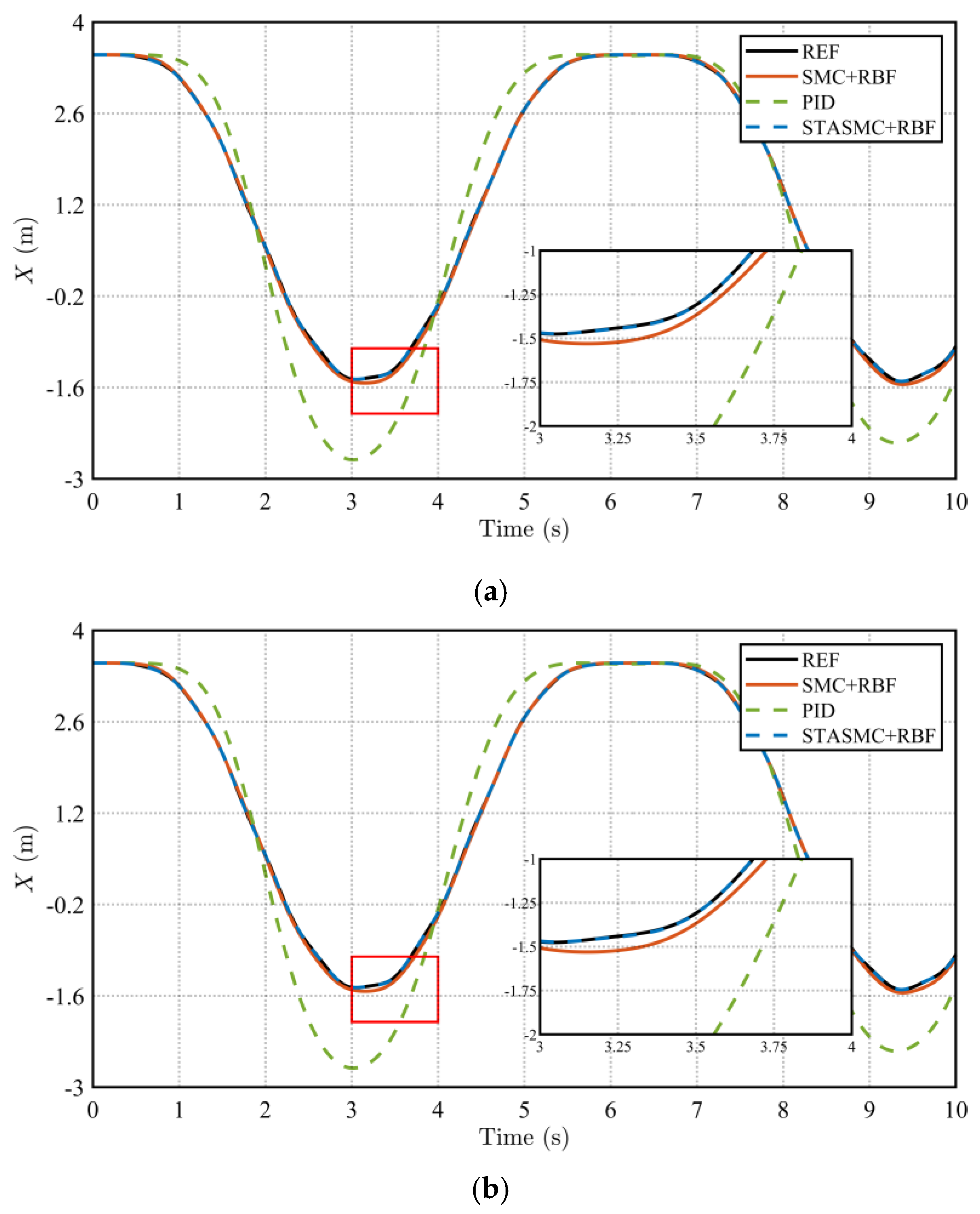
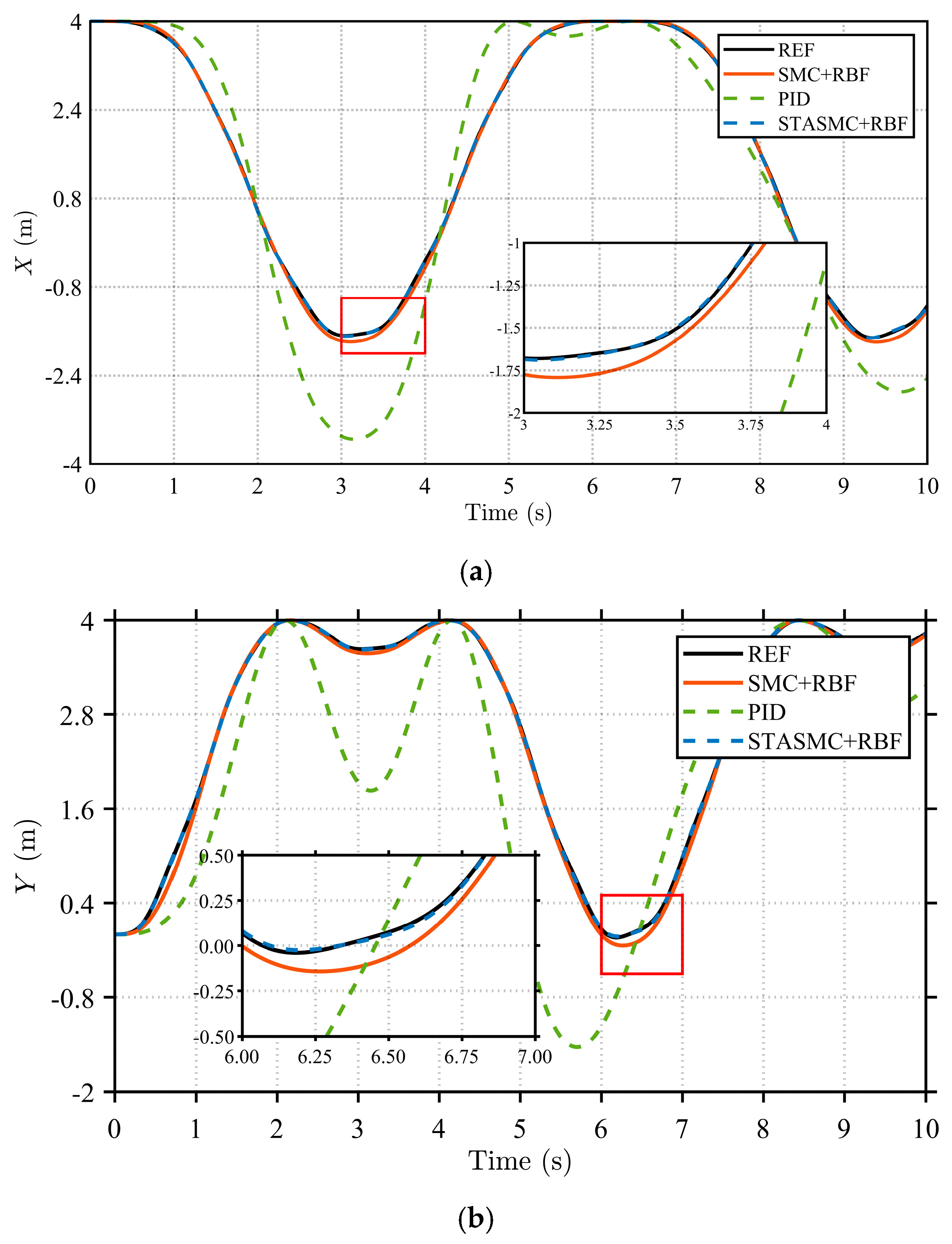
The trajectory tracking accuracy of the flexible load’s end-effector serves as a key metric for evaluating system control precision. The X and Y axis trajectories of the spatial flexible manipulator are illustrated in Figure 4.

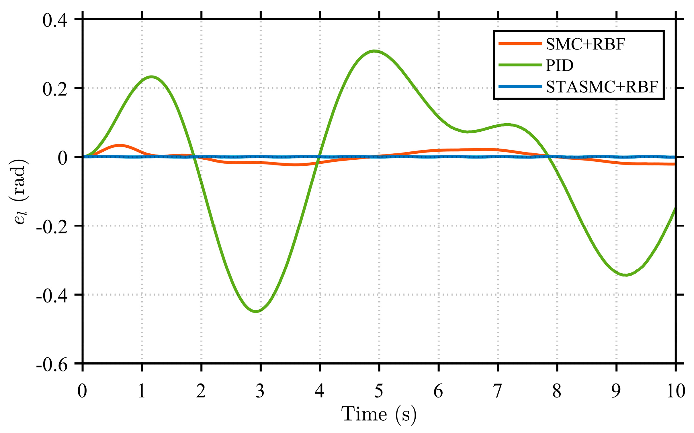
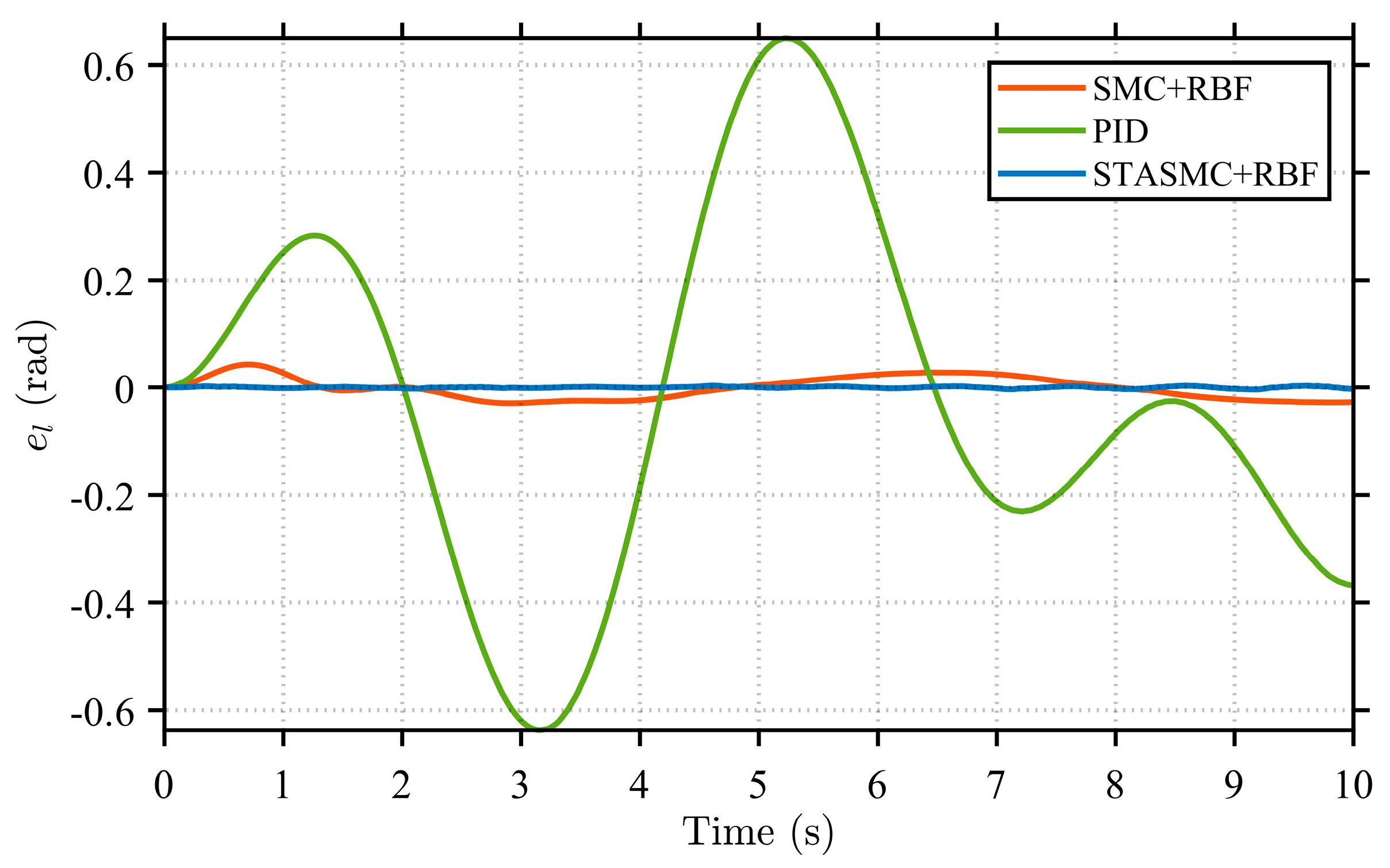
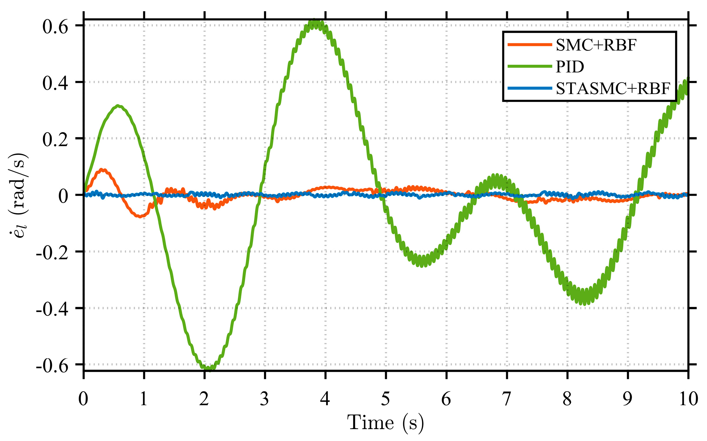
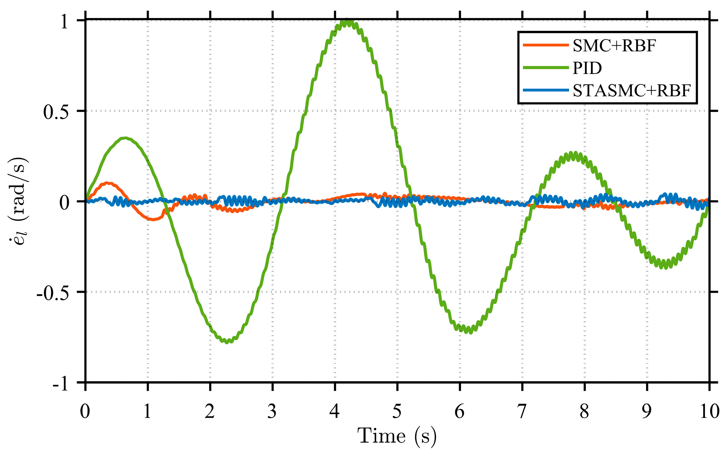
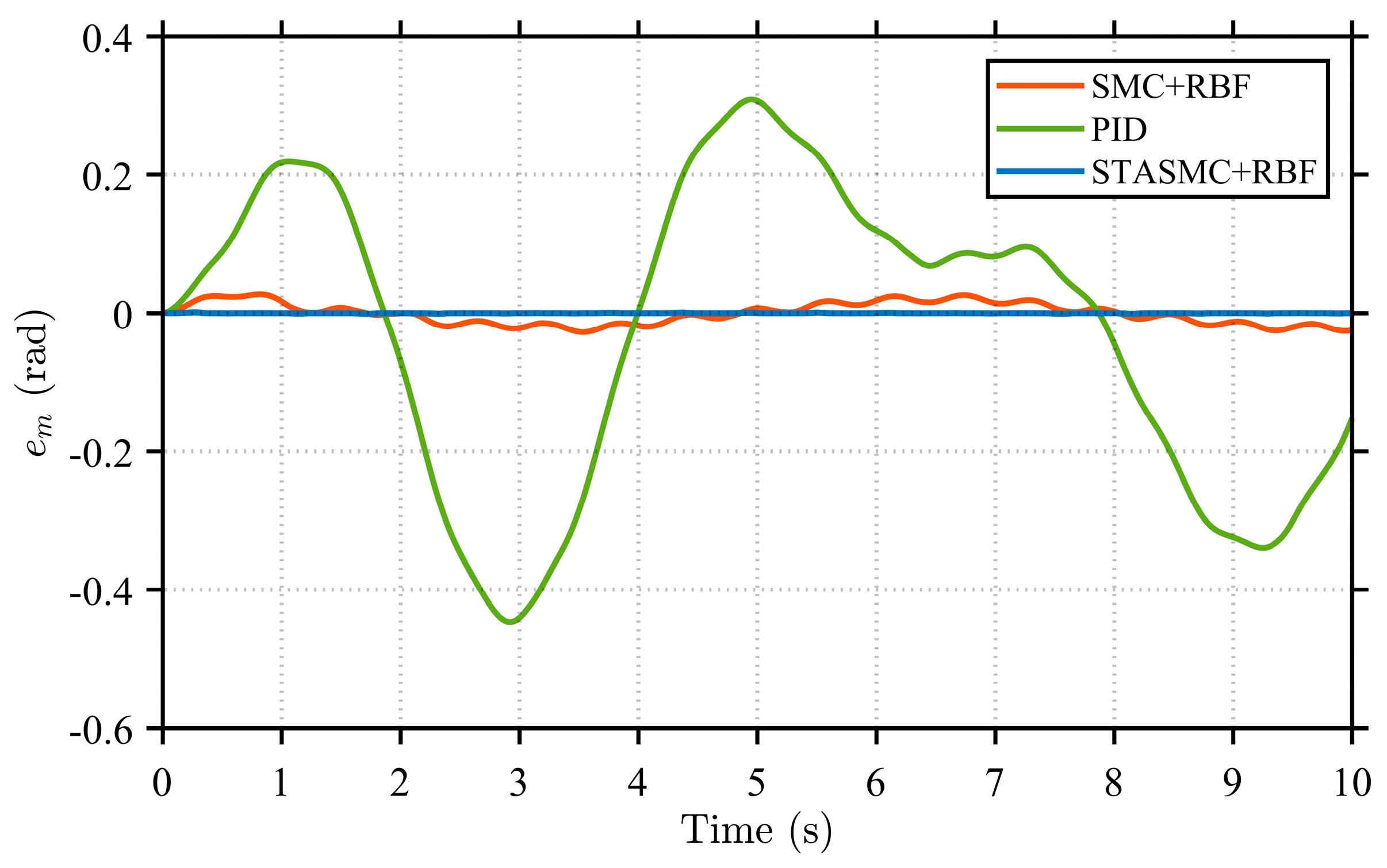
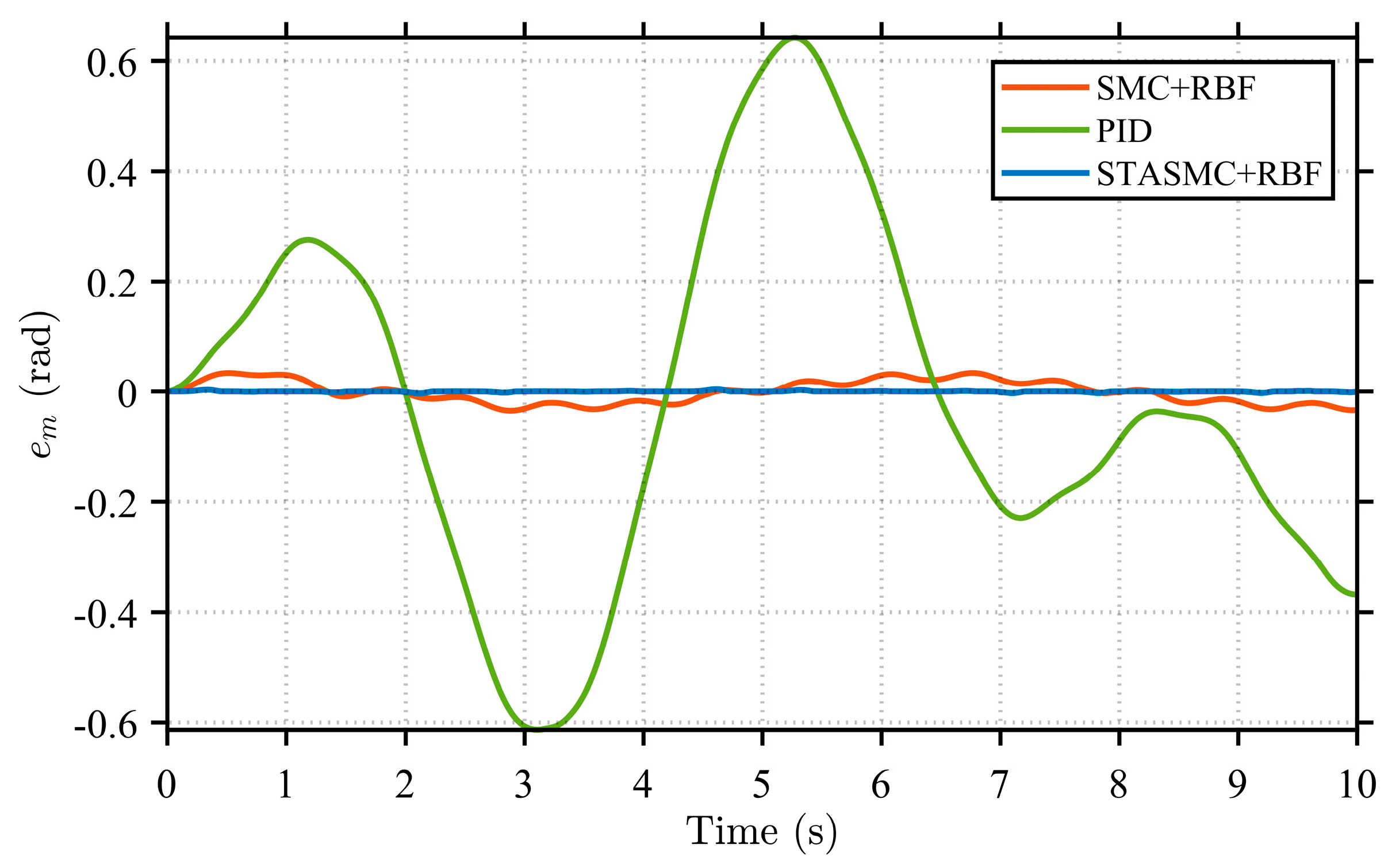
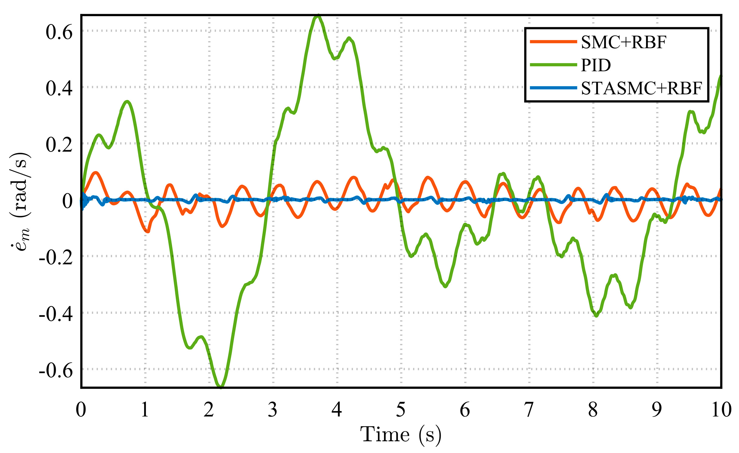
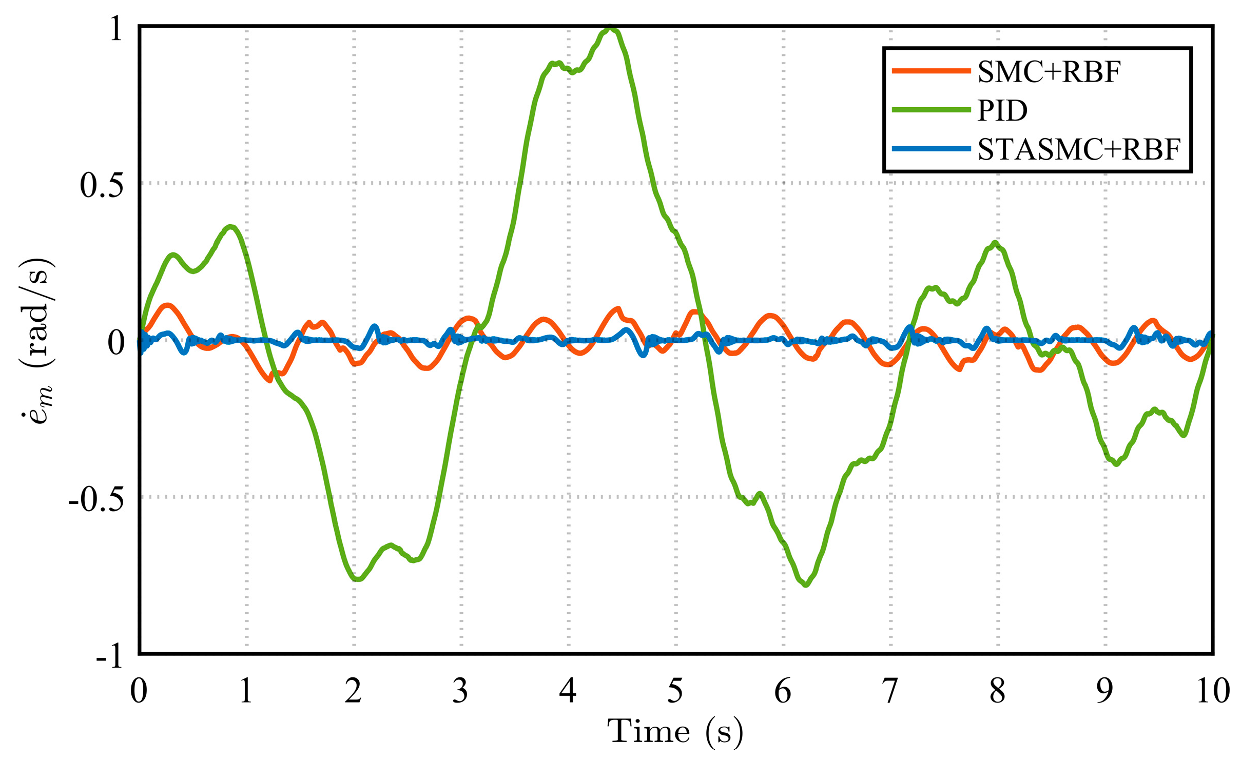
In Figure 4, REF represents the desired trajectory. A comparison of the simulation results reveals clear discrepancies between the desired trajectory and the actual tracking trajectories under different control strategies. The PID control exhibits sustained and significant deviations in both the X and Y axis directions, with its trajectory consistently failing to align closely with the desired path. This reflects the inherent limitations of PID in handling complex nonlinear systems and disturbances. In contrast, the SMC strategy improves tracking performance to some extent; however, its deviation increases further during turning and acceleration phases. The STASMC + RBF strategy demonstrates superior trajectory tracking performance. Overall, the path tracked by STASMC + RBF almost coincides with the desired trajectory, showing no noticeable lag. Further observation of the local magnified view confirms that STASMC + RBF achieves precise tracking in both the X and Y axis directions without significant oscillation or deviation at turns. By comparison, the trajectory under SMC exhibits continuous minor deviations and jitter, indicating the inferior convergence of the sliding surface and disturbance rejection capability relative to the STASMC + RBF structure. As shown in Figure 5, the proposed STASMC + RBF strategy maintains an excellent trajectory tracking performance across different operating conditions. To quantitatively evaluate accuracy and further highlight the advantages of the proposed strategy, the rotation angle error (Figure 6 and Figure 7) and angular velocity error (Figure 8 and Figure 9) at the flexible load end, as well as the rotation angle error (Figure 10 and Figure 11) and angular velocity error (Figure 12 and Figure 13) at the servo motor end, are compared for the three control strategies under the same operating condition. These metrics respectively reflect the disturbance suppression capability of the flexible load and the control precision of the actuator.

The rotation angle and angular velocity error curves at both the load end and motor end, shown in Figure 6, Figure 7, Figure 8, Figure 9, Figure 10, Figure 11, Figure 12 and Figure 13, clearly demonstrate the performance differences among the control strategies. Regarding rotation angle errors, the PID control strategy exhibits significant deviations throughout the entire time range. Its error curves show considerable fluctuations with large amplitudes, presenting persistent asymmetric oscillations at both the load end and motor end. This observation further confirms the limited capability of the PID strategy in suppressing disturbances in nonlinear systems, resulting in relatively unstable system performance. In comparison, the SMC + RBF strategy exhibits relatively regular periodic fluctuations in its error curves, with reduced amplitude compared to the PID strategy. This indicates that its variable structure control mechanism enhances robustness against parameter variations and disturbances, demonstrating certain insensitivity characteristics. Additionally, with the adaptive compensation capability of the RBF neural network, the SMC + RBF strategy achieves the better identification and suppression of uncertainties in the system. However, the SMC + RBF strategy still exhibits some level of chattering, which is also reflected in the continuous fluctuations of its angular velocity error curves. Furthermore, the error performance of the three control strategies under various conditions is presented, with a focus on the angle and angular velocity errors of the flexible load. It can be observed that as the manipulator arm length increases, the amplitudes of both the steering angle error and the angular velocity error exhibit an increasing trend. This indicates intensified system vibration under the extended arm configuration. Despite this, the STASMC + RBF-based control strategy consistently demonstrates significantly narrower error bounds. In contrast, both the conventional SMC + RBF and PID strategies exhibit larger oscillation amplitudes and more pronounced fluctuations in steering angle error.

To quantitatively evaluate the advanced advantages of the proposed control strategy, this paper selects the rotation angle error $\mathrm{el}$ and the angular velocity error $\dot{\mathrm{e}}l$ at the load end for comparative analysis, as shown in

Table 2. Comparison of performance metrics for control strategies.

	Control Strategy	Condition	RMSE	MAE	RMSE Reduction
Angle error of flexible load ($\mathrm{el}$)	SMC + RBF	1	0.0131	0.0104	-
	STASMC + RBF	1	0.0005	0.0004	96.3%
	SMC + RBF	2	0.0178	0.0142	-
	STASMC + RBF	2	0.0015	0.0012	91.4%
Rotating angular velocity error of flexible load ($\dot{\mathrm{e}}l$)	SMC + RBF	1	0.0255	0.0202	-
	STASMC + RBF	1	0.0045	0.0037	82.3%
	SMC + RBF	2	0.0352	0.0277	-
	STASMC + RBF	2	0.0138	0.0110	60.8%

. The rotation angle error $\mathrm{el}$ directly determines the absolute positioning accuracy of the end-effector, serving as a key static parameter for evaluating trajectory tracking performance. In contrast, the angular velocity error $\dot{\mathrm{e}}l$ reflects the dynamic smoothness during motion, whose fluctuations are directly related to issues such as the residual oscillation of the flexible load and operational chattering.

Given that the preceding simulation results clearly show a significant performance gap (by orders of magnitude) between conventional PID control and the sliding-mode-based strategies for both error types, the comparison is focused on two RBF-enhanced sliding mode variants, namely, the conventional sliding mode control with RBF neural network (SMC + RBF) and the proposed super-twisting sliding mode control with RBF neural network (STASMC + RBF). This approach excludes the vastly underperforming PID baseline, allowing for a more precise examination of the unique improvements brought by the STASMC structure.

For quantitative comparison, Table 2 lists the root mean square error (RMSE) and mean absolute error (MAE) for both strategies under different operating conditions. RMSE is more sensitive to larger errors, effectively characterizing the dispersion of the error distribution, while MAE provides a robust estimate of the absolute error level. As the data in Table 2 indicate, under the two conditions with different load lengths, the STASMC + RBF strategy exhibits significantly lower RMSE and MAE values for both el and el compared to the SMC + RBF strategy. Specifically, under Condition 1, STASMC + RBF reduces the RMSE of el by 96.3% and that of $\dot{\mathrm{e}}l$ by 82.3%. Under the more challenging Condition 2 (with increased arm length), it still achieves reductions of 91.4% and 60.8%, respectively. These quantitative results demonstrate that the STASMC + RBF strategy not only shows a clear advantage in improving end-point positioning accuracy, but is also highly effective in suppressing velocity fluctuations and vibrations. Furthermore, the strategy maintains superior performance under varying parameters (load length), demonstrating its enhanced robustness.

In summary, the STASMC + RBF control strategy demonstrates excellent performance in all aspects. Both its rotation angle and angular velocity error curves maintain minimal amplitudes throughout, with overall smoother variations and no significant chattering or sustained oscillations. By introducing integral operations, the super-twisting algorithm’s architecture suppresses high-frequency switching, leading to smooth disturbance compensation and output. Furthermore, the STASMC + RBF strategy shows good consistency in the error curves at both the load end and the motor end, indicating effective cooperative control between the two ends and improved overall tracking accuracy and synchronization performance. Therefore, it can be concluded that the RBF neural network-based super-twisting algorithm sliding mode control strategy achieves high control precision in reducing system chattering and minimizing rotation angle and velocity errors.

5. Practical Implementation Considerations and Challenges

Although the theoretical effectiveness of the proposed super-twisting sliding mode control strategy has been validated via numerical simulations in this study, its deployment on a real physical system presents a series of critical challenges in transitioning from a simulation to an engineering application. This section systematically outlines the core implementation issues, including hardware integration constraints, real-time software implementation, and engineering-oriented parameter tuning, discussing potential challenges for subsequent experimental research and practical application.

5.1. Hardware Integration and Vibration Feedback Challenges

The implementation of the theoretical control law strictly relies on the accurate and real-time feedback of the system states. In a practical variable-length dual-flexibility servo system, this requires at least the synchronized acquisition of the servo motor rotation angle and a physical quantity characterizing the flexible deformation at the load end. The motor rotation angle can be directly obtained from an integrated high-precision encoder; however, the direct measurement of the transverse deformation or vibration acceleration of the load constitutes a primary difficulty. As the second derivative of deformation, acceleration is directly related to vibration intensity and residual oscillation [26]. Selecting the acceleration signal as the carrier for vibration feedback is a feasible strategy.

5.2. Real-Time Control Software Implementation

The simulation verification was completed within the MATLAB(2021a)/Simulink environment, while the final deployment relies on a real-time hardware platform such as NI cRIO-9030 and the LabVIEW(2025 Q1) programming environment. This transition involves significant platform migration challenges. The implementation of complex control algorithms—particularly modules containing the RBF neural network’s online adaptation law and the super-twisting differentiation operations—requires addressing a series of engineering issues when porting to graphical or real-time operating systems like LabVIEW. These include code refactoring, deterministic and periodic task scheduling, hardware driver compatibility, and memory management.

5.3. Parameter Tuning and Computational Complexity

The controller parameters tuned based on the ideal simulation model require readjustment and validation on the actual hardware platform. The gains of the super-twisting control, the learning rate of the RBF neural network, and the coefficients of the robust term collectively form a multi-dimensional parameter space. The tuning process for these parameters is complex and coupled. Simultaneously, the computational complexity of the algorithm must match the finite computational resources of the controller. The forward propagation and weight update of the RBF network, as well as the continuous non-smooth operations potentially involved in the super-twisting control law, all impose demands on the processor’s computing power and execution efficiency. How to adjust parameters from the ideal model and balance computational complexity with control performance is key to ensuring robustness in practical operation.

In summary, successfully deploying the control strategy proposed in this paper from the simulation environment to a physical experimental platform is a systems engineering task involving multi-disciplinary aspects such as mechatronics design, software engineering, signal processing, and system identification. The challenges encountered validate the robustness requirements of theoretical algorithms under practical conditions. It is hoped that the discussion of these key implementation issues in this study will provide a useful reference for subsequent control strategy design and engineering deployment oriented toward practical applications.

6. Conclusions

This paper investigates a spatially flexible manipulator considering system uncertainties, for which dynamic equations are formulated. To enhance control precision and mitigate chattering in sliding mode control, a super-twisting algorithm sliding mode control strategy is proposed. In contrast to existing approaches that modify switching functions or employ disturbance observers for external compensation, the proposed method incorporates higher-order sliding mode concepts and integral terms to inherently reduce chattering. Additionally, an RBF neural network is utilized to identify and compensate for uncertainties by leveraging its universal approximation capability for nonlinear functions. This multi-faceted approach effectively suppresses control-induced chattering. The simulation results demonstrate that the proposed neural network-based super-twisting algorithm sliding mode control strategy significantly improves system control accuracy.

References

1. Rahimi Nohooji, H.; Voos, H. Compliant Robotics in Space: A Prospective Review of Soft and Deformable Systems for Space Missions. Adv. Intell. Syst. 2025, 7, 2400785. [Google Scholar] [CrossRef]
2. Shang, D.; Li, X.; Yin, M.; Li, F. Vibration suppression for two-inertia system with variable-length flexible load based on neural network compensation sliding mode controller and angle-independent method. IEEE/ASME Trans. Mechatron. 2022, 28, 848–859. [Google Scholar] [CrossRef]
3. Shang, D.; Li, X.; Yin, M.; Li, F. Dynamic modeling and fuzzy compensation sliding mode control for flexible manipulator servo system. Appl. Math. Model. 2022, 107, 530–556. [Google Scholar] [CrossRef]
4. Gupta, N.; Pratiher, B. Dynamic modeling and effective vibrati-on reduction of dual-link flexible manipulators with two-stage cascade PID and active torque actuation. Mech. Mach. Theory 2025, 205, 105867. [Google Scholar] [CrossRef]
5. Long, T.; Li, E.; Hu, Y.; Yang, L.; Fan, J.; Liang, Z.; Guo, R. A vibration control method for hybrid-structured flexible manipulator based on sliding mode control and reinforcement learning. IEEE Trans. Neural Netw. Learn. Syst. 2020, 32, 841–852. [Google Scholar] [CrossRef]
6. Li, S.; Meng, L.; Fang, K.; Liu, F. Neural Network Adaptive Inve-rse Control of Flexible Joint Space Manipulator Considering the Influence of Gravity. Sensors 2024, 24, 6942. [Google Scholar] [CrossRef]
7. Liu, Y.; An, S.; Wang, L.; Fan, Z. Predefined time sliding mode tracking control of autonomous underwater vehicles with uncertainties and disturbances. Ocean Eng. 2025, 331, 121318. [Google Scholar] [CrossRef]
8. Ahmed, S.; Ahmed, A.; Mansoor, I.; Junejo, F.; Saeed, A. Output feedback adaptive fractional-order super-twisting sliding mode control of robotic manipulator. Iran. J. Sci. Technol. Trans. Electr. Eng. 2021, 45, 335–347. [Google Scholar] [CrossRef]
9. Han, Z.; Zhang, K.; Yang, T.; Zhang, M. Spacecraft fault-tolerant control using adaptive non-singular fast terminal sliding mode. IET Control Theory Appl. 2016, 10, 1991–1999. [Google Scholar] [CrossRef]
10. Wang, Y.; Li, S.; Wang, D.; Ju, F.; Chen, B.; Wu, H. Adaptive time-delay control for cable-driven manipulators with enhanced nonsingular fast terminal sliding mode. IEEE Trans. Ind. Electron. 2020, 68, 2356–2367. [Google Scholar] [CrossRef]
11. Mohd Zaihidee, F.; Mekhilef, S.; Mubin, M. Robust speed control of PMSM using sliding mode control (SMC)—A review. Energies 2019, 12, 1669. [Google Scholar] [CrossRef]
12. Wang, L.; Shi, Q.; Liu, J.; Zhang, D. Backstepping control of flexible joint manipulator based on hyperbolic tangent function with control input and rate constraints. Asian J. Control 2020, 22, 1268–1279. [Google Scholar] [CrossRef]
13. Van, M.; Ge, S.S.; Ren, H. Finite time fault tolerant control for robot manipulators using time delay estimation and continuous nonsingular fast terminal sliding mode control. IEEE Trans. Cybern. 2016, 47, 1681–1693. [Google Scholar] [CrossRef] [PubMed]
14. Zhang, J.; Meng, W.; Yin, Y.; Li, Z.; Ma, L.; Liang, W. High-order sliding mode control for three-joint rigid manipulators based on an improved particle swarm optimization neural network. Mathematics 2022, 10, 3418. [Google Scholar] [CrossRef]
15. Levant, A. Robust exact differentiation via sliding mode technique. Automatica 1998, 34, 379–384. [Google Scholar] [CrossRef]
16. Zuo, Y.; Mei, J.; Zhang, X.; Lee, C.H.T. Simultaneous identification of multiple mechanical parameters in a servo drive system using only one speed. IEEE Trans. Power Electron. 2020, 36, 716–726. [Google Scholar] [CrossRef]
17. Kim, S. Moment of inertia and friction torque coefficient identification in a servo drive system. IEEE Trans. Ind. Electron. 2018, 66, 60–70. [Google Scholar] [CrossRef]
18. Zhao, Z.; Liu, Z. Finite-time convergence disturbance rejection control for a flexible Timoshenko manipulator. IEEE/CAA J. Autom. Sin. 2020, 8, 157–168. [Google Scholar] [CrossRef]
19. Lee, H.; Utkin, V.I. Chattering suppression methods in sliding mode control systems. Annu. Rev. Control 2007, 31, 179–188. [Google Scholar] [CrossRef]
20. He, C.; Zhang, F.; Jiang, J. Adaptive boundary control of flexible manipulators with parameter uncertainty based on RBF neural network. Shock Vib. 2020, 2020, 8261423. [Google Scholar] [CrossRef]
21. Shang, D.; Li, X.; Yin, M.; Li, F. Model identification control strategy for coupled elastic joint flexible load drive system based on NNSMC controller and new deformation description. J. Frankl. Inst. 2023, 360, 6357–6401. [Google Scholar] [CrossRef]
22. Yang, H.; Liu, J. An adaptive RBF neural network control method for a class of nonlinear systems. IEEE/CAA J. Autom. Sin. 2018, 5, 457–462. [Google Scholar] [CrossRef]
23. Gao, H.; He, W.; Zhou, C.; Sun, C. Neural network control of a two-link flexible robotic manipulator using assumed mode method. IEEE Trans. Ind. Inform. 2018, 15, 755–765. [Google Scholar] [CrossRef]
24. Gaultier, P.E.; Cleghorn, W.L. A spatially translating and rotating beam finite element for modeling flexible manipulators. Mech. Mach. Theory 1992, 27, 415–433. [Google Scholar] [CrossRef]
25. De Wit, C.C.; Olsson, H.; Astrom, K.J.; Lischinsky, P. A new model for control of systems with friction. IEEE Trans. Autom. Control 1995, 40, 419–425. [Google Scholar] [CrossRef]
26. Shang, D.; Li, X.; Yin, M.; Li, F. Dynamic modeling and control for dual-flexible servo system considering two-dimensional deformation based on neural network compensation. Mech. Mach. Theory 2022, 175, 104954. [Google Scholar] [CrossRef]
Figure 1. Schematic of the spatial flexible manipulator structure.
Applsci 16 00387 g001
Figure 2. Deformation representation of the spatial flexible manipulator.
Applsci 16 00387 g002
Figure 3. Control block diagram of the spatial flexible manipulator system.
Applsci 16 00387 g003
Figure 4. Schematic of X and Y axes trajectories under condition 1. (a) X axis trajectory diagram; (b) Y axis trajectory diagram.
Applsci 16 00387 g004
Figure 5. Schematic of X and Y axes trajectories under condition 2. (a) X axis trajectory diagram; (b) Y axis trajectory diagram.
Applsci 16 00387 g005
Figure 6. Rotation angle error of the flexible load under condition 1.
Applsci 16 00387 g006
Figure 7. Rotation angle error of the flexible load under condition 2.
Applsci 16 00387 g007
Figure 8. Angular velocity error of the flexible load under condition 1.
Applsci 16 00387 g008
Figure 9. Angular velocity error of the flexible load under condition 2.
Applsci 16 00387 g009
Figure 10. Rotation angle error of the servo motor under condition 1.
Applsci 16 00387 g010
Figure 11. Rotation angle error of the servo motor under condition 2.
Applsci 16 00387 g011
Figure 12. Angular velocity error of the servo motor under condition 1.
Applsci 16 00387 g012
Figure 13. Angular velocity error of the servo motor under condition 2.
Applsci 16 00387 g013