Author Contributions
Conceptualization, Q.Y., D.D. and T.Z.; Methodology, Q.Y., F.M., Q.W. and Z.F.; Software, F.M. and Z.F.; Validation, T.Z.; Formal analysis, Q.W.; Resources, Q.Y. and D.D.; Writing—original draft, Q.Y. and T.Z.; Writing—review & editing, F.M., Q.W., Z.F. and T.Z. All authors have read and agreed to the published version of the manuscript.
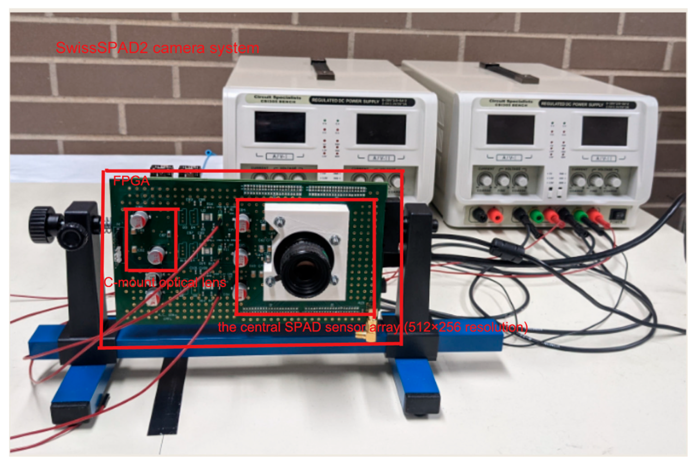
Figure 1.
The SwissSPAD2 camera system (EPFL, Lausanne, Switzerland) used for real-world data acquisition. Although visually compact, the setup integrates several critical components: the central SPAD sensor array (512 × 256 resolution) coupled with a high-speed FPGA controller (bottom board) for binary frame buffering, and a C-mount optical lens assembly (front) for light collection. The system transmits binary photon streams via a USB 3.0 interface to the host workstation for subsequent SNR-guided enhancement and depth reconstruction processing.
Figure 2.
Sample low-light input images from the LOL-v1 dataset. These images are characterized by low contrast and significant noise. Note: For visualization purposes, the brightness of these images has been increased using gamma correction (γ = 2.2) to make the contents visible.
Figure 2.
Sample low-light input images from the LOL-v1 dataset. These images are characterized by low contrast and significant noise. Note: For visualization purposes, the brightness of these images has been increased using gamma correction (γ = 2.2) to make the contents visible.
Figure 3.
Corresponding normal-light ground truth images for the LOL-v1 dataset shown in
Figure 2. These high-quality reference images are used to supervise the training of the enhancement network.
Figure 3.
Corresponding normal-light ground truth images for the LOL-v1 dataset shown in
Figure 2. These high-quality reference images are used to supervise the training of the enhancement network.
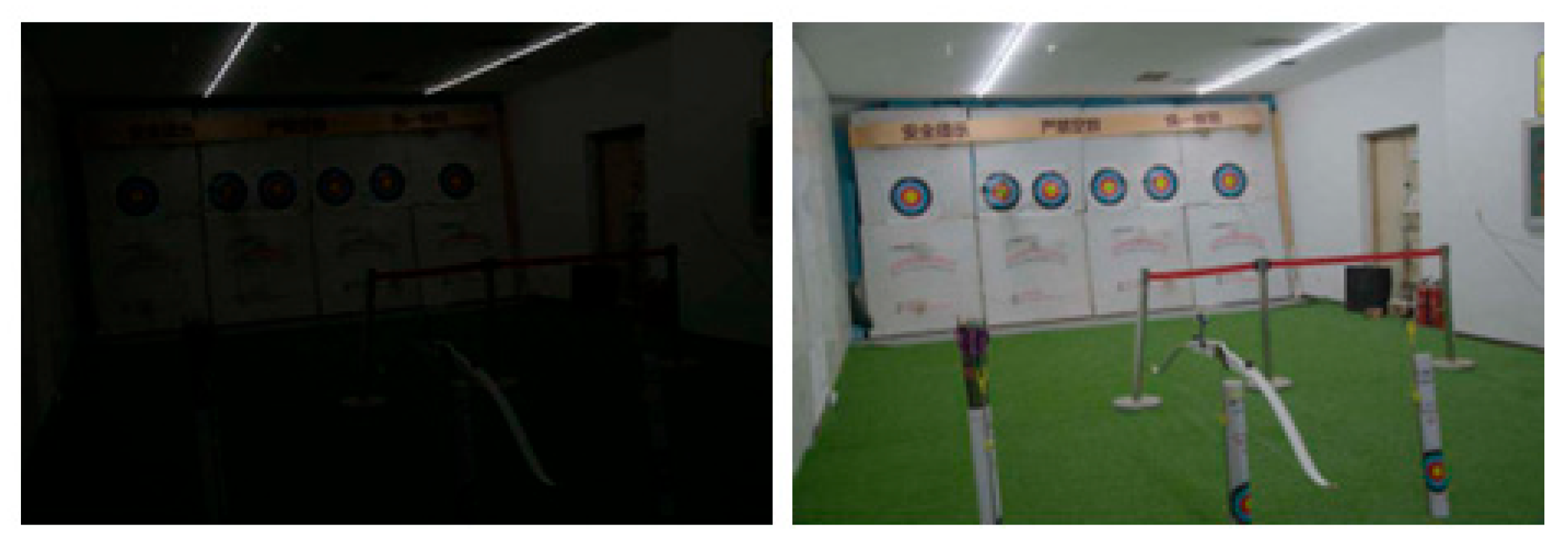
Figure 4.
Representative low-light input samples from the LOL-v2 dataset. The scenes include varying illumination conditions that challenge standard enhancement algorithms. (Gamma correction applied for visibility).
Figure 4.
Representative low-light input samples from the LOL-v2 dataset. The scenes include varying illumination conditions that challenge standard enhancement algorithms. (Gamma correction applied for visibility).
Figure 5.
Corresponding normal-light ground truth images for the LOL-v2 real subset shown in
Figure 4. These high-quality reference images provide the target supervision signal, enabling the network to learn accurate color restoration and detail enhancement during training. Note: The non-English text appearing on the posters in the background consists of safety slogans inherent to the original scene and is not relevant to the image enhancement metrics.
Figure 6.
Representative low-light input samples from the LOL-v2 dataset. The scenes include varying illumination conditions that challenge standard enhancement algorithms. (Gamma correction applied for visibility). The low visibility and noise are characteristics of the low-light input data.
Figure 6.
Representative low-light input samples from the LOL-v2 dataset. The scenes include varying illumination conditions that challenge standard enhancement algorithms. (Gamma correction applied for visibility). The low visibility and noise are characteristics of the low-light input data.
Figure 7.
High-quality reference images from the LOL-v2 synthetic dataset. These serve as the ground truth, from which low-light versions were synthesized by simulating noise and illumination degradation. Comparing results against these images allows for precise quantitative evaluation of the model’s generalization ability.
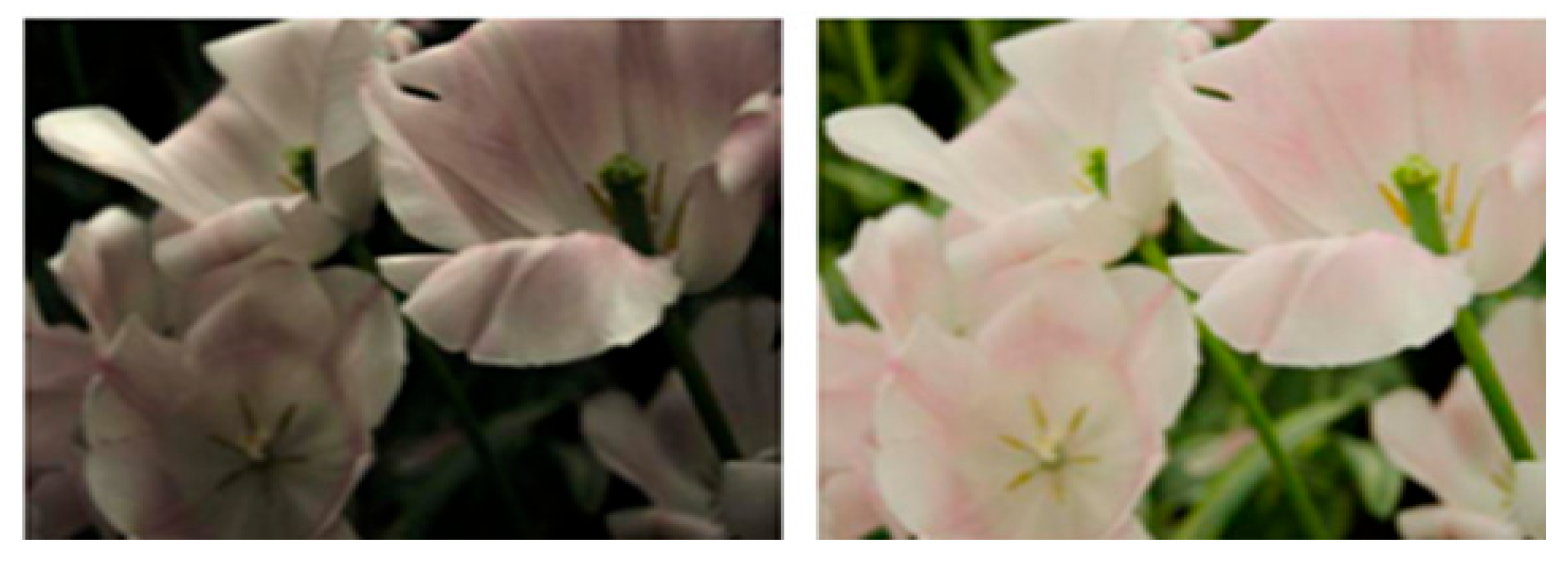
Figure 8.
Paired samples from the SID dataset. The left/top images show the short-exposure (low-light) inputs, which suffer from extreme noise and color distortion. The right/bottom images show the corresponding long-exposure ground truth.
Figure 8.
Paired samples from the SID dataset. The left/top images show the short-exposure (low-light) inputs, which suffer from extreme noise and color distortion. The right/bottom images show the corresponding long-exposure ground truth.
Figure 9.
Representative sample scenes from the SMID dataset used in our evaluation. This dataset features dynamic scenes captured under extreme darkness, providing paired data consisting of short-exposure noisy inputs and corresponding long-exposure ground truth images (shown here) to benchmark performance in real-world motion scenarios. The images are displayed in standard RGB true color, and the center image features a color checker chart used for color reference.
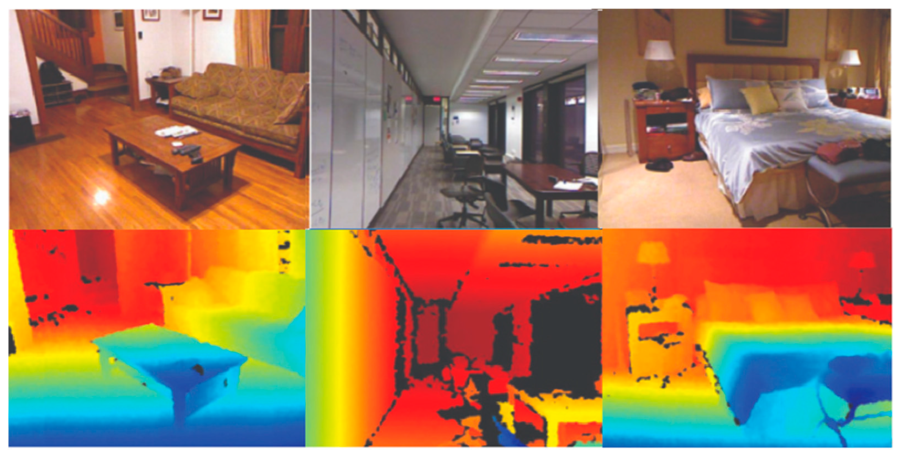
Figure 10.
Representative samples from the NYU Depth V2 dataset. The top row displays the input RGB images of indoor scenes, while the bottom row shows the corresponding ground truth depth maps (visualized as heatmaps). These samples are used to evaluate the depth estimation branch of the proposed framework. In the depth maps, the color gradient represents distance from the camera, where blue indicates near objects and red indicates far objects.
Figure 11.
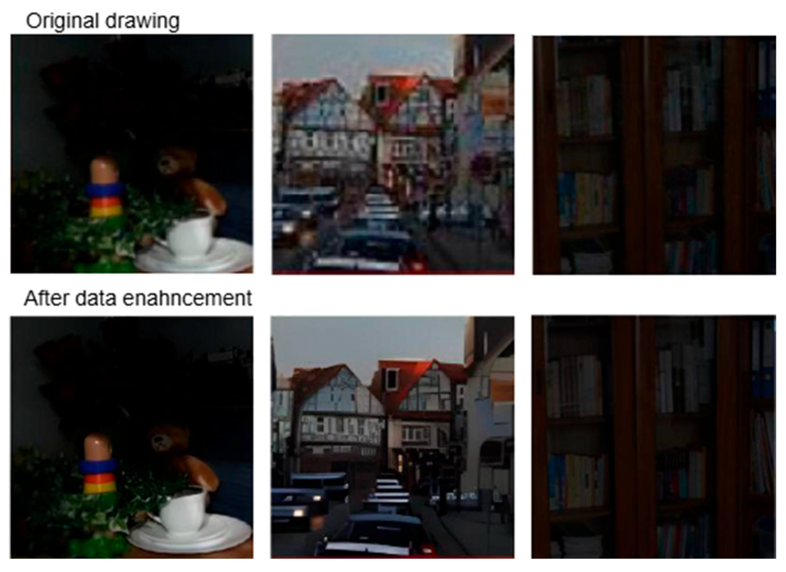
Visual comparison of image enhancement results. (Top row): Original low-light inputs (displayed with digital gain), showing severe noise and loss of detail. (Bottom row): Enhanced results generated by our proposed SNR-guided framework. Our method effectively suppresses noise while recovering structural details and accurate colors, verifying the effectiveness of the proposed data augmentation and enhancement strategy.
Figure 12.
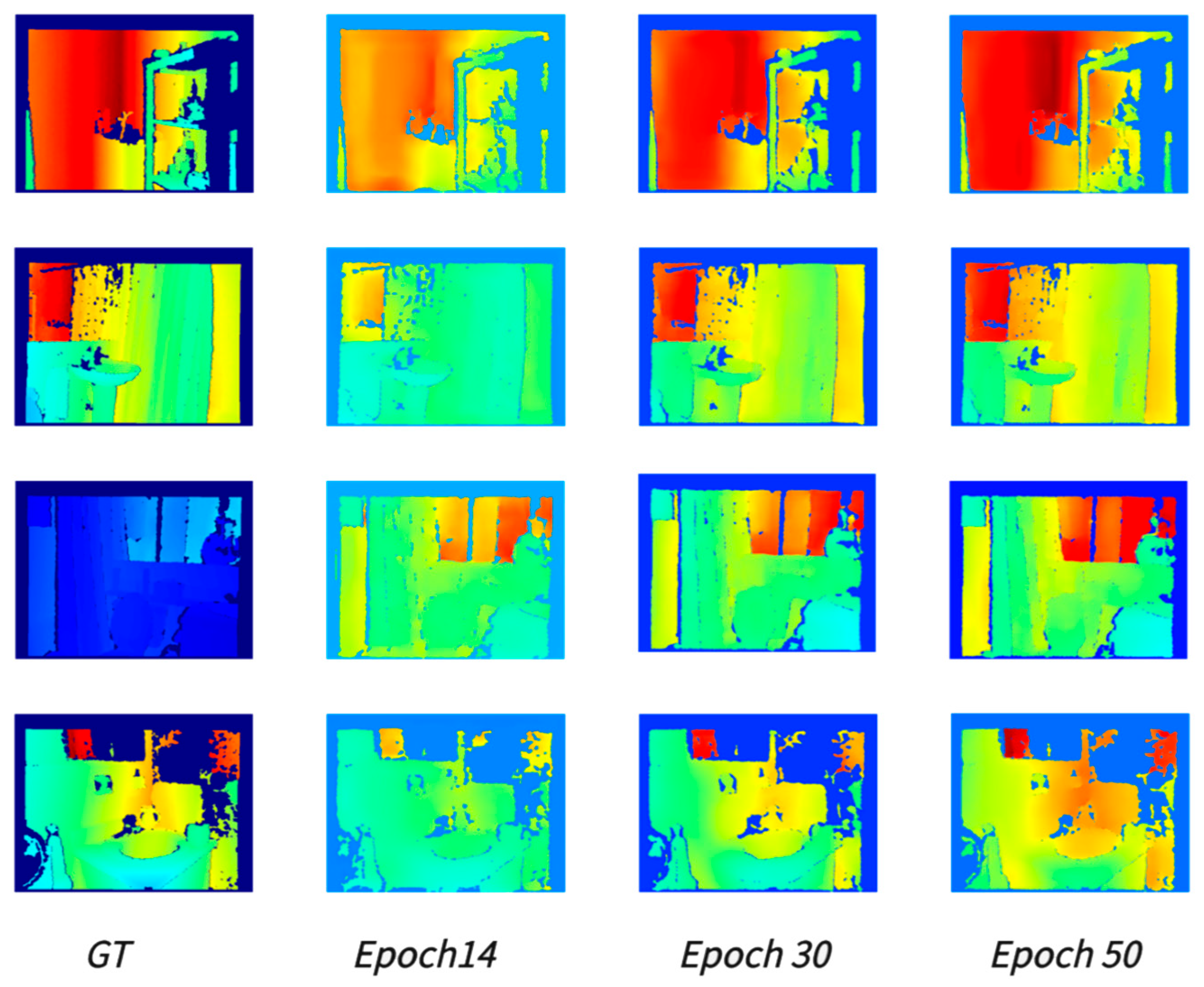
Visualization of the VQGAN reconstruction process across different training epochs. From (left) to (right): The Ground Truth (GT) image, and the reconstructed outputs at Epoch 14, Epoch 30, and Epoch 50. As training progresses, the model (at Epoch 50) demonstrates superior capability in preserving high-frequency textures and edge details compared to earlier stages. The depth maps are visualized using a false-color heatmap, where blue represents near distances and red represents far distances.
Figure 13.
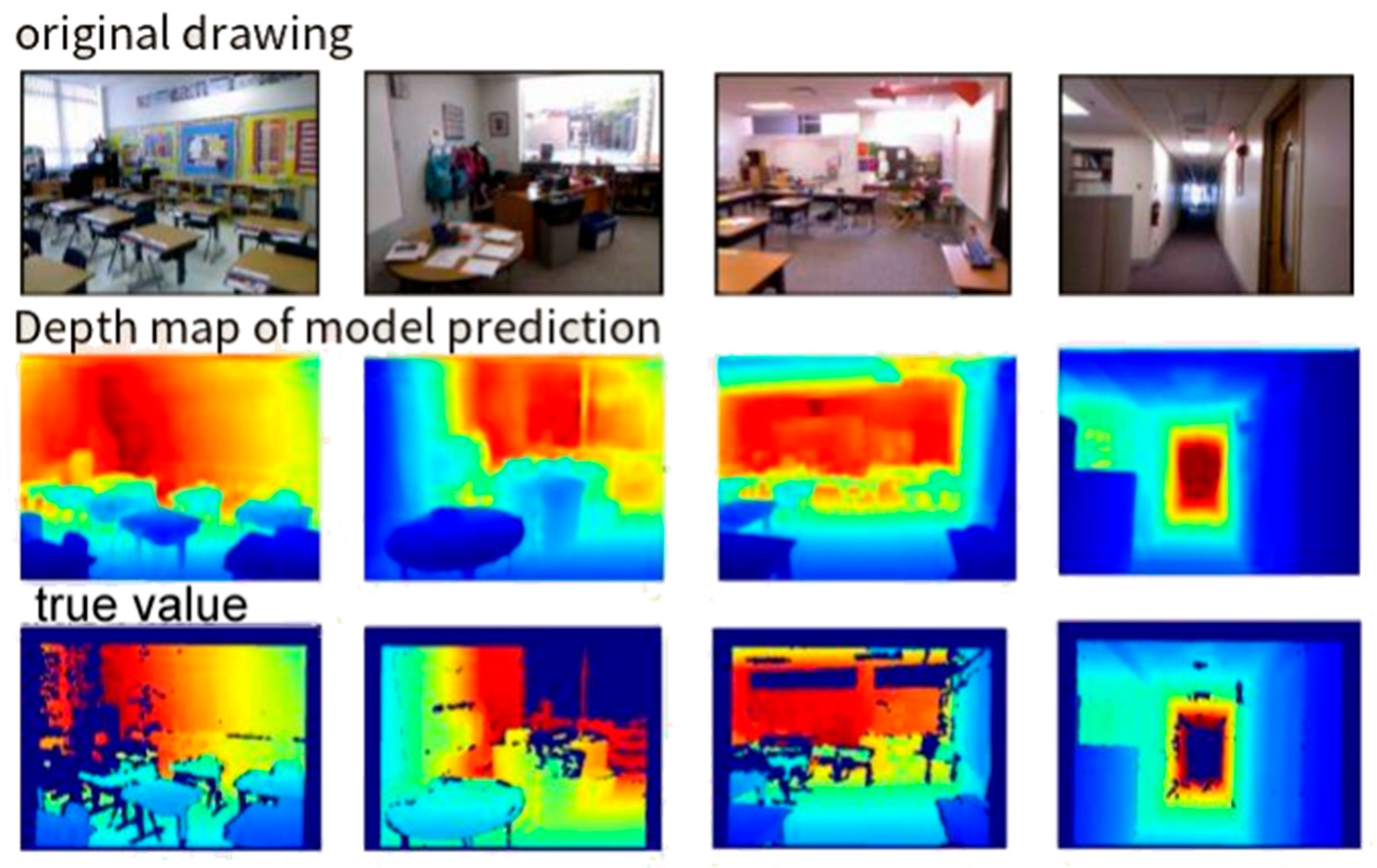
Qualitative results of depth estimation on the NYU Depth V2 dataset. The figure compares the Ground Truth depth maps (Left/Top) with the Predicted depth maps (Right/Bottom) generated by our autoregressive model. The results show that our model accurately infers depth gradients and object boundaries even in complex scenes. The depth maps are visualized as heatmaps, where blue indicates near distances and red indicates far distances.
Figure 14.
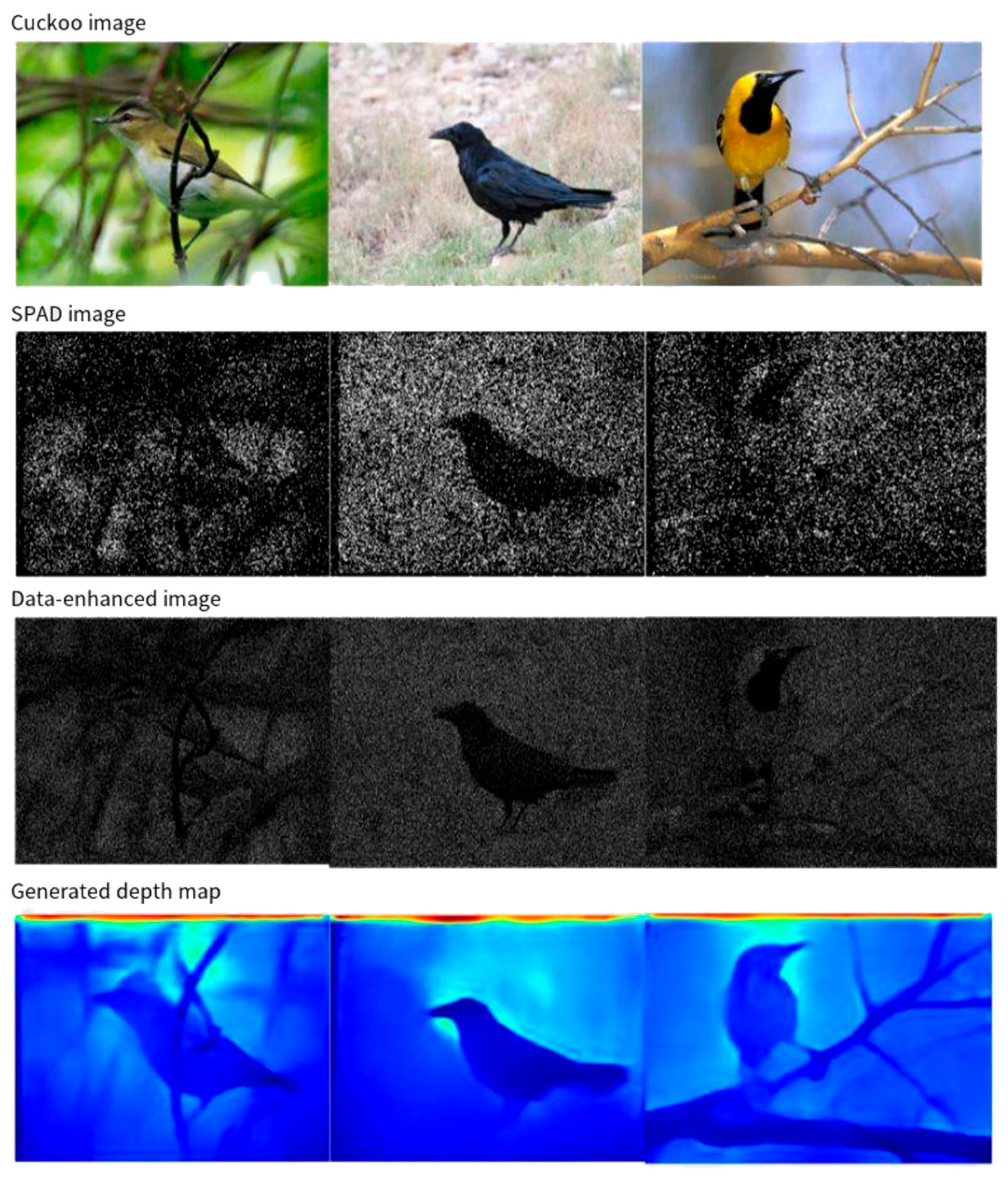
Comprehensive evaluation on real-world single-photon data (CUB-200-2011 subset) captured by SwissSPAD2. From (top) to (bottom): (1) The reference monitor image; (2) The raw captured SPAD image, characterized by extreme noise and sparsity; (3) The data-enhanced image restored by our SNR-guided module; and (4) The generated depth map. This demonstrates the framework’s robustness in recovering visual content and estimating depth from actual photon-limited sensors. The depth maps are visualized as heatmaps, where blue indicates near distances and red indicates far distances.
Table 1.
Comparison of image enhancement performance.
Table 1.
Comparison of image enhancement performance.
| | LOL-v1 | LOL-v2-r | LOL-v2-s | SID |
|---|
| Methods | PSNR | SSIM | PSNR | SSIM | PSNR | SSIM | PSNR | SSIM |
|---|
| LPNet | 21.46 | 0.802 | 17.80 | 0.792 | 19.51 | 0.846 | 20.08 | 0.598 |
| MIR-Net | 24.14 | 0.830 | 20.02 | 0.820 | 21.94 | 0.876 | 20.84 | 0.605 |
| Retinex | 18.23 | 0.720 | 18.37 | 0.723 | 16.55 | 0.652 | 18.44 | 0.581 |
| IPT | 16.27 | 0.504 | 19.80 | 0.813 | 18.30 | 0.811 | 20.53 | 0.561 |
| Ours | 24.61 | 0.842 | 21.48 | 0.849 | 24.14 | 0.928 | 22.87 | 0.625 |
Table 2.
Depth estimation results.
Table 2.
Depth estimation results.
| ↑ | ↑ | ↑ | ↓ | ↓ | ↓ |
|---|
| Joint Denoising | 0.671 | 0.896 | 0.967 | 0.209 | 1.412 | 0.087 |
| Photon Net | 0.713 | 0.917 | 0.976 | 0.183 | 1.275 | 0.078 |
| ours | 0.725 | 0.941 | 0.984 | 0.162 | 1.177 | 0.069 |
Table 3.
Performance on real single-photon data.
Table 3.
Performance on real single-photon data.
| ↑ | ↑ | ↑ | ↓ | ↓ | ↓ |
|---|
| Joint Denoising | 0.660 | 0.878 | 0.934 | 0.256 | 1.476 | 0.092 |
| Photon Net | 0.682 | 0.924 | 0.941 | 0.197 | 1.293 | 0.084 |
| ours | 0.721 | 0.961 | 0.976 | 0.171 | 1.184 | 0.074 |
Table 4.
Ablation study results of different modules in the low-light image enhancement framework.
Table 4.
Ablation study results of different modules in the low-light image enhancement framework.
| | LOL-v1 | LOL-v2-r | LOL-v2-s | SID |
|---|
| Methods | PSNR | SSIM | PSNR | SSIM | PSNR | SSIM | PSNR | SSIM |
|---|
| Ours w/o L | 16.27 | 0.638 | 16.98 | 0.687 | 20.81 | 0.881 | 19.10 | 0.593 |
| Ours w/o S | 23.06 | 0.828 | 18.98 | 0.790 | 23.47 | 0.919 | 22.30 | 0.604 |
| Ours w/o SA | 20.67 | 0.752 | 18.85 | 0.765 | 21.88 | 0.842 | 21.02 | 0.544 |
| Ours w/o A | 21.86 | 0.760 | 19.40 | 0.782 | 22.23 | 0.866 | 21.19 | 0.550 |
| Ours | 24.61 | 0.842 | 21.48 | 0.849 | 24.14 | 0.928 | 22.87 | 0.625 |
Table 5.
Ablation study results of different training strategies for the autoregressive model.
Table 5.
Ablation study results of different training strategies for the autoregressive model.
| Training Strategies | ↑ | ↓ | ↓ |
|---|
| Frozen Training | 0.706 | 0.249 | 1.309 |
| Low-Rank Adaptation (LoRA) | 0.718 | 0.208 | 1.224 |
| Full Fine-tuning | 0.763 | 0.162 | 1.177 |
Table 6.
Ablation results for different control encoder configurations.
Table 6.
Ablation results for different control encoder configurations.
| Control Encoder | ↑ | ↓ | ↓ |
|---|
| CNN | 0.685 | 0.248 | 1.459 |
| ViT-S | 0.714 | 0.256 | 1.287 |
| DINOv2-S | 0.720 | 0.258 | 1.279 |
| VQGAN | 0.725 | 0.162 | 1.177 |
Table 7.
Ablation results for control fusion strategies.
Table 7.
Ablation results for control fusion strategies.
| Fusion Strategies | Layer | ↑ | ↓ | ↓ |
|---|
| Cross-Attention Fusion | 1-th | 0.721 | 0.168 | 1.179 |
| Direct Additive Fusion | 1-th | 0.714 | 0.171 | 1.205 |
| Direct Additive Fusion | 1,5,9-th | 0.725 | 0.162 | 1.177 |
| Direct Additive Fusion | 1∼12-th | 0.720 | 0.165 | 1.184 |
