1. Introduction
Public transport is a more affordable and sustainable alternative to solo personal vehicle travel due to its lower fares and its mitigative effect on urban congestion and pollution [
1,
2]. Therefore, several developing countries, such as India, are turning to trains (metro rail) to reduce urban congestion due to their higher passenger carrying capacity [
3]. However, despite such large infrastructure investments in metro trains, actual ridership levels have fallen far below the targets in many cities [
4]. Therefore, identifying and addressing key deterrents to the demand for metro services becomes an urgent priority in order to resolve urban mobility challenges. In this direction, this study proposes a joint model for train demand that is based on both disaggregate consideration probability at the individual level, as well as the aggregate hourly station demand.
Several studies globally have shown that existing forecasts for metro demand are highly optimistic, whereas the realized demand is much lower. For example, Bhattacharjee et al. (2020) noted a substantial shortfall in daily metro ridership compared to the projections in Indian cities, such as Bengaluru (50% shortfall), Chennai (80% shortfall), and Jaipur (90% shortfall) [
5]. Similar challenges are observed in neighboring South Asian countries, as well as the U.S. and Europe. For instance, in Dhaka, Bangladesh, mass rapid transit is used for 10% to 20% of short- to medium-distance trips [
6]. In the U.S., Los Angeles and Houston metros fall short of their projected ridership by 30% and 80%, respectively [
7,
8]. European urban rail projects have a 20% gap between forecasted and actual ridership [
9]. These trends highlight the global challenge in achieving the expected rail transit ridership.
The shortfall in train ridership may arise from either a demand deficit at the disaggregate choice level or a lower-than-expected aggregate ridership. At the disaggregate level, some individuals may not even include or consider trains in their choice set. Consideration is an initial and essential stage of demand since it captures the behavioral intent of travelers to include this mode in their choice set. This dimension can be viewed as an indicator of potential demand and comprises the expanded user base of regular users, as well as infrequent travelers. The consideration probability for the metro is influenced by factors including growing personal vehicle ownership, poor walkability, and low accessibility to train stations [
10,
11]. Hence, effective policy interventions are necessary to encourage non-users to consider and shift to train travel.
On the other hand, footfall represents the second or subsequent stage of demand, which is conditional on the consideration that reflects the realized demand or the actual extent of metro usage. The conventional literature on transportation mainly focuses on aggregated measures, such as footfall, boarding, or alighting at stations, representing indicators of the realized demand. This measure reflects the intensity of use and is influenced more by transit attributes such as fare reduction or increasing service frequency. Also, such aggregate demand may be influenced by factors such as (i) poor transit operational characteristics, such as low frequency or high fares [
12,
13], (ii) inadequate station characteristics, including limited parking availability and complex navigation within the station [
14], (iii) insufficient accessibility to the station through poor first- and last-mile connectivity and non-usable footpaths [
15], and (iv) a lack of attractive land-use or built environment characteristics near the station [
16].
The existing studies on metro demand focus either on the realized demand through ridership metrics or the potential demand through disaggregate consideration probabilities. Both approaches present only a partial picture of actual metro usage due to the following limitations. Aggregate demand models suffer from self-selection bias, as they rely solely on data from metro users and overlook the responses of non-users. Additionally, they cannot quantify the effect of intra-station variables (e.g., first- and last-mile connectivity and land use), and individual-level variables (e.g., socio-economic characteristics, work characteristics, and user perceptions) that vary across respondents within the same buffer area in a metro station [
10,
17]. In addition, most existing aggregate demand models use unidirectional measures, such as boarding or alighting, which do not provide a comprehensive indication of demand for terminal planning or first- and last-mile service design. These limitations can lead to inaccurate or misleading estimates of demand.
Conversely, disaggregate models of consideration and choice can overcome self-selection bias and capture intra-station and inter-person variables. However, their sample sizes are smaller compared to the aggregate demand data used from the automated fare collection (AFC) data. Also, these disaggregate models capture the behavioral intent of travelers to include the metro in their choice set, but not their actual usage level. Hence, they cannot be used for forecasting ridership or revenue estimates.
The above discussion highlights the need for investigating both these stages of demand and their interactions, which are overlooked in the literature. A clear distinction between the aforementioned potential and realized demand dimensions becomes essential from a policy perspective. By improving the consideration propensities, transit agencies may be able to expand their user base, whereas interventions focused on footfall can enhance ridership. Thus, there is a need for different policy levers to address these dimensions. For example, it is plausible that out-of-vehicle attributes, as well as accessibility, could affect consideration, whereas in-vehicle experiences and station amenities could affect ridership.
By explicitly modeling the two dimensions and their interactions, this study aims to examine the following research questions that are underexplored: (i) which segments show a deficit in consideration probabilities, and through what factors can they be enhanced? (ii) How do intra-station and inter-personal variables affect aggregate footfall demand? (iii) What is the role of self-selection bias in the aggregate demand model? (iv) Whether and to what extent does disaggregate consideration probability have a mediating effect on realized footfall? (v) At what locations does footfall remain low despite a high consideration rate, and how can this be mitigated? (vi) Are segment-specific, location-specific, and dimension-specific (consideration vs. footfall) policies more effective than uniform ones in enhancing demand?
To address these research issues, the following objectives are pursued in this study.
- (1)
To propose a framework for the joint analysis of both disaggregate consideration probabilities and aggregate footfall outcomes.
- (2)
To investigate the behavioral differences in consideration propensity outcomes, using market segments based on personal mobility resource availability.
- (3)
To investigate the interdependence between potential demand (disaggregate consideration) and realized demand (aggregate footfall) outcomes, with particular attention to distinguishing the role of key variables across the two dimensions.
- (4)
To illustrate the differential impacts of policy interventions across consideration and footfall dimensions.
These objectives are investigated based on empirical data from Chennai City, India, using two main data sources: footfall data from the automated fare collection (AFC) system at metro stations and mode consideration data from a household survey. Footfall is defined here as the total number of passengers entering and exiting the train station (sum of hourly boarding and alighting) during a given time period. The two datasets are used to propose a joint modeling framework investigating the interplay between consideration probability and aggregate footfall, comprising two interrelated models: (i) a binary logit model for metro train consideration probabilities and (ii) a non-linear Box–Cox model for station-level footfall.
This study contributes to the existing literature on metro demand evaluation in the following respects. A comprehensive and novel characterization of metro service usage patterns is proposed by modeling two distinct stages of potential and realized demand and their interactions. The stages comprise (i) disaggregated consideration probability reflecting the behavioral intent to use the metro and (ii) aggregate footfall that represents actual usage intensity. This novel model addresses the self-selection bias present in aggregate demand models due to their neglect of non-user data. Heterogeneity in user preferences towards multimodal connectivity and transit service characteristics based on personal mobility segments is captured at the disaggregate level. In addition, this study evaluates the effect of individual-level variables and intra-station variables on the footfall dimension, which is overlooked in existing aggregate models. The results highlight the differential influence of key variables across the consideration and footfall dimensions. Two sources of non-linear effects in the footfall dimension are captured using a Box–Cox transformation and through the mediating effect of the consideration propensity. Neglecting these features leads to biased estimates, poorer model fits, and misleading policy implications. The practical significance of this model is empirically illustrated by showing the dimension-specific and location-specific impacts of alternative policies to enhance multimodal integration.
The rest of the paper is organized as follows:
Section 2 synthesizes the related literature regarding disaggregate and aggregate train demand models. The data used in this study and the associated exploratory analysis are described in
Section 3.
Section 4 describes the proposed joint model formulation and specification. The results and findings are presented in
Section 5, followed by a discussion of policy implications in
Section 6. Finally, the last concluding section highlights the important findings and contributions from this study.
2. Literature Review
This section synthesizes the literature on existing transit demand models, with a focus on disaggregate consideration and choice as indicators of the potential demand, as well as the aggregate demand as a measure of the realized or actual usage, followed by a summary of key knowledge gaps that motivated this study.
2.1. Disaggregate Demand Models on Transit Consideration and Mode Choice
Disaggregate demand models focus on individual choice outcomes and can be classified into two broad categories: (i) consideration models and (ii) binary and multinomial mode choice models. The main findings from these studies are summarized in the following subsections.
2.1.1. Research on Train Consideration
Consideration models focus on the process of including an alternative in the choice set of many alternatives [
18]. Consideration is affected by feasibility, availability, awareness, and compatibility with activity–travel patterns. These models are developed using either a latent variable approach or revealed choice data [
17,
19,
20]. Such revealed data typically consists of binary variables about whether a particular mode was used within a specified time window [
21,
22]. Among the two approaches, for existing modes, modeling the revealed outcome is often preferable, as it is easier for respondents to report, and the response is more precise than corresponding latent variable indicators. However, selecting an appropriate time window for measuring consideration is essential for robust model development. Measurements over very long time windows may lead to poor memory recall by respondents or may not accurately reflect recent travel patterns. On the other hand, consideration over just a few days may capture some rare or occasional trips but may not reflect regular patterns.
Regardless of whether a latent or observed variable approach is used, almost all studies assume that consideration of a particular mode is a binary response variable. Hence, it is widely modeled using binary logit or probit models, and the main empirical findings are summarized below. In many such models, accessibility characteristics are found to strongly affect the propensity of individuals to consider trains. For example, high access and egress distances (or walk time) reduce the propensity to consider trains [
10,
11]. Outwater et al. (2012) identified that individuals unwilling to walk for more than two minutes were unlikely to consider trains [
17]. However, there is not enough understanding of how perceptions of footpath usability and the ease of walking access to train stations affect consideration. Furthermore, research on access and egress times for modes other than walking is scarce. In particular, the impact of intermediate public transport (IPT) modes, such as auto-rickshaws and shared autos (regular or ride-hailing), on train consideration is not well understood. This is especially important for Indian cities, where IPT modes carry a significant number of passengers to train stations daily.
Vehicle ownership is often regarded as a major inhibitor to considering public transit. The literature reveals that vehicle ownership reduces the likelihood of considering trains [
10,
11]. Another study illustrated that individuals who are captive to public transit due to vehicle unavailability have a higher propensity to consider trains [
11]. However, the role of vehicle type, number, and degree of availability in train consideration has not received adequate attention. Notably, none of these studies explored whether the sensitivity to factors such as first- and last-mile connectivity, walkability, or perceptions towards train services varies across different market segments based on the availability of personal vehicles.
Quantitative transit service attributes (e.g., travel time, cost) and the qualitative level of service for the train services (e.g., comfort, crowding) play a key role in deciding whether individuals include trains in their choice set [
10]. Outwater et al. (2012) showed that individuals who perceived low comfort levels in transit were less likely to consider train services [
17]. Additionally, those with a pro-transit attitude were more likely to consider the train. However, the influence of these factors could vary across market segments, which remains underexplored. For example, individuals owning a car may prioritize comfort over cost [
23], whereas those owning a two-wheeler might be more sensitive to travel time.
Empirical studies have also revealed the effect of socio-demographic variables on train consideration. For example, younger individuals, females, and high-income respondents were more likely to consider trains than other segments [
17,
20]. However, research attention to differences in station-level characteristics (including terminal facilities, amenities in the neighborhood, etc.) is needed.
2.1.2. Binary and Multinomial Mode Choice Models for Transit Demand
Several studies have utilized binary logit models to explore whether commuters use transit or not [
24,
25,
26]. Selvakumar et al. (2023) revealed that suburban rail passengers prioritize fare differences over travel time savings [
27]. Chiu et al. (2014) identified accessibility and transit time as key factors influencing rail mode choice [
28]. Similar studies were carried out for urban buses, as well. Zhou et al. (2014) investigated factors influencing bus choice for different distances, finding that long-distance commuters prioritize comfort and safety, medium-distance commuters focus on travel time and headway, and short-distance travelers focus on punctuality and distance to the bus station [
25]. Anwar and Yang (2017) highlighted travel time as a crucial factor in mode choice between buses and cars [
24]. They reported that direct bus service policies were observed to be more impactful than park-and-ride facilities in enhancing the Wollongong bus system. Puan et al. (2019) highlighted that bus reliability positively influenced choice, whereas income had a negative impact [
26].
The shortcoming of binary choice models is that they disregard the characteristics and availability of other means of travel, especially if the data is collected over a short period, such as a single day. To relax these limitations of binary models, many studies have employed multinomial models of transit choice. Empirical findings indicate the significance of in-vehicle travel time, out-of-vehicle travel time, and travel cost [
6]. Furthermore, subjective factors, such as positive perceptions regarding comfort and crowding levels inside buses, encourage public transit use [
29]. Additionally, this study also found that some commuters shift from private vehicles to the metro because of its cost-effectiveness and time savings, compared to private vehicles.
Although disaggregate choice models offer better spatial representation of home and work locations, they suffer from small sample sizes and fail to capture transit usage frequency. Thus, they identify individual differences and non-user responses to policies but do not fully explain footfall. Moreover, the influence of first- and last-mile connectivity, walkability, travel perceptions, and personal or work characteristics on metro consideration remains underexplored across segments.
2.2. Aggregate Demand Models for Metro Train Services
Boarding, alighting, ridership, and footfall are some of the most commonly used measures to model aggregate demand, typically aggregated at hourly, daily, or annual levels. Footfall is a comprehensive indicator that captures bi-directional station flows and offers a finer resolution than run-level measures, such as ridership or occupancy [
14,
30]. Linear regression is widely used for modeling aggregate demand [
14,
15]. However, some studies have highlighted the violations of the normality assumption, and hence have opted for log-transformed linear regression models [
13]. Such log–linear models are still constrained in some respects, and their performance with regard to other non-linear specifications remains underexplored.
Mucci and Erhardt (2018) used a non-linear Transit Direct Ridership (TDR) model to investigate the effect of supply and demand factors on daily rail ridership [
13]. Their results showed that the demand indicators, such as employment and housing density, positively influence rail ridership. The frequency of transit also showed a positive impact on train ridership, which is expected. Durning and Townsend (2015) explored the role of socio-economics, stations, service, neighborhood, and land use attributes on transit ridership [
15]. Their model found no impact of socio-demographic factors, but accessibility measures, such as park-and-ride facilities and feeder bus services, were significant. However, the role of the qualitative and quantitative aspects of supporting pedestrian and bicycle infrastructure, such as the quality of footpaths and the availability of public cycle docking stations, has received relatively less attention in the literature. Lastly, affordability and quality of transit service affect ridership in the expected direction [
13,
14].
Researchers have used ridership models to evaluate policy interventions aimed at increasing rail ridership. These interventions range from flexible fare systems or awareness programs to increasing fleet size or introducing new transit modes at access, line-haul, or egress stages. A study in South East Queensland, Australia, found that fare reduction and other incentives increased public transport ridership by 1.32% [
12]. Similarly, Liu et al. (2016) recommended transit-oriented development around boarding points and improvements in safety and reliability at each stage to enhance transit demand [
14].
Aggregate demand models, typically based on automated fare collection (AFC) or automated passenger counting (APC) data, offer large samples but suffer from self-selection bias, as they include only transit users. This exclusion prevents them from capturing the preferences and behaviors of non-users. Additionally, their aggregated nature makes it difficult to account for individual characteristics, spatial effects within stations, and multimodal connectivity. While linear and log–linear models are commonly used, non-linear approaches remain underexplored. Most studies focus on inter-station factors like connectivity between stops, but pay less attention to intra-station elements like terminal characteristics and surrounding land use. Furthermore, these models do not consider the interdependence between consideration decisions and ridership.
2.3. Summary of Gaps
Table 1 summarizes the key gaps in the literature. The existing studies have not simultaneously modeled potential demand and realized demand outcomes, which limits the ability to distinguish the effects of key variables on disaggregate consideration and aggregate footfall demand. The interaction between these two aspects also remains poorly understood. Additionally, there is a lack of policies tailored to specific locations, user segments, and demand dimensions. To address these gaps, this study aims to quantify and distinguish the factors that discourage people from considering metro rail from those factors that reduce the intensity of metro use among people who consider it. To achieve this, a novel joint modeling framework is developed, integrating disaggregate consideration data from household surveys with aggregate footfall data from AFC, as detailed in the following sections.
3. Data Collection and Exploratory Data Analysis
Three main data sources are utilized in this study. The first source is individual surveys, which are used to model train consideration. These surveys also collected information on respondents’ socio-demographic characteristics, perceptions of transit services, first- and last-mile connectivity, and walkability. The second source comprises automated fare collection (AFC) data from 32 metro stations in Chennai that capture weekday footfall. The third source is secondary data, including official timetables from Chennai Metro Rail Limited and the Metropolitan Transport Corporation to obtain metro and bus service frequency and headway details [
32,
33]. Additionally, secondary data from the Chennai City Master Plan and Google Maps Points-of-Interest (PoIs) are used to determine population density and land-use variables [
34]. A detailed discussion of the data and exploratory analysis is presented next.
3.1. The Data Description for the Consideration Model
A model predicting train consideration probability, as an indicator of potential demand, was developed using data from a face-to-face household survey of about 815 commuters in Chennai City during 2015–2016 [
21]. After data cleaning and assembly, 803 valid responses were obtained. This sample size is adequate based on sample size calculations [
35], as it is larger than the required sample size of 666 respondents for a 5% relative error margin and 99% confidence interval (i.e., Z = 2.58), assuming an average consideration propensity (
p = 0.5). This consideration probability was selected for calculation as it gives the highest possible variance and the largest required sample size. The survey was conducted using stratified random sampling across 12 zones, covering urban, peri-urban, and suburban areas in Chennai. The sample size in each zone was proportional to its population, relative to the total population of the selected zones.
Figure 1a shows the survey zones, and
Figure 1b presents the residential and workplace locations of the respondents, demonstrating good spatial coverage of the study sample used to analyze potential demand.
The survey collected data on commute modes considered in the three months prior to the survey date and the primary mode chosen for work trips. Additionally, the respondents provided information on factors hypothesized to influence their decision to consider the train, such as first- and last-mile connectivity, walkability, perceptions of transit service, and socio-demographic characteristics, using the following scales:
- (i)
First- and Last-Mile Factors (FLMs): include the access and egress time, distance, and cost to reach nearby public transport stations.
- (ii)
Walkability-Related Variables (WLKs): assess footpath usability on an ordinal scale (low, medium, or high) and the ease of walking or crossing roads near railway stations (low, medium, or high).
- (iii)
Perception of Train Service Characteristics (TSCs): evaluate the comfort, security, and ease of purchasing tickets (each rated as low, medium, or high) and the availability of amenities, such as shops or restaurants, near train stations (yes/no).
- (iv)
Personal and Work-Related Characteristics (PERWs): include variables such as age, gender, income, and work distance.
The sample was found to be reasonably representative of the key variables. The average household size in the sample was 4.0, closely matching the population value of 4.1 in 2011 [
36]. The average monthly household income ranged between INR 10,000 and INR 20,000. The average number of two-wheelers and cars per household was 1.22 and 0.27, respectively, aligning with the population average of 1.26 across vehicles in 2008 [
21]. The primary mode share for work commutes in the sample consisted of 61% personal vehicles (two-wheelers and cars), 28% public transit (bus and train), 7% intermediate public transport (IPT), including auto-rickshaws, shared autos, and company-provided services, and 4% non-motorized transport (walking and cycling). Additionally, the average commute distance was 11.4 km, with a median travel duration of approximately 45 min for home-to-work trips.
This study defines train consideration as a binary variable indicating whether a respondent used the train within the three months before the survey. This operationalization, using recent usage, serves as a tangible proxy for identifying individuals for whom the train is a relevant part of their active choice set, ensuring that the most recent, as well as sufficiently consistent travel patterns, are captured, without compromising recall accuracy. It is to be noted that the definition for including the metro in a choice set, while conceptually aligned with the potential demand, was based on revealed preference rather than solely on stated preference. Specifically, inclusion required the respondents to have reported using the metro at least once in the preceding three months. Therefore, this measure not only represents potential demand, i.e., consideration or choice set inclusion, but also has a direct influence on the realized demand, i.e., footfall, as the individuals meeting this criterion have demonstrably used the train system.
Overall, only one-third of the respondents reported considering the train during this period, indicating a stronger preference for other transport modes. Next, the differences in consideration rates across the segments based on the number, type, and exclusive availability of a motorized vehicle were examined (
Figure 2).
For this, the respondents were categorized into three categories. Those without vehicles or driving knowledge formed the captive group. Individuals owning only one two-wheeler, but who do not have exclusive access (i.e., vehicle is shared among multiple household members), are referred to as semi-captive travelers. The rest of the respondents had a motorized vehicle available for their exclusive use and were referred to as choice riders. Even within this group, individuals who owned only one two-wheeler and had exclusive access are termed as the two-wheeler choice riders and are considered a different sub-category compared to car-owning choice riders.
Figure 2 shows that the share of individuals considering trains varies substantially across these segments. The semi-captive group has the highest consideration share (45%), suggesting that the potential demand is highest in this segment and is an important segment for promoting train usage. Interestingly, captive users had a consideration rate for the train (33%), which is less than the semi-captive respondents, probably because buses and shared autos are more accessible and less expensive than metro trains in Chennai (mean access distance to bus stop vs. train station is 0.5 km vs. 2.8 km, respectively). Thus, for this segment, the competition between public transit modes (bus and train) needs to be minimized through appropriate integration policies. Among choice riders, those with only a two-wheeler have a 32% train consideration rate, whereas car owners have a slightly lower rate of 30%. For this group, the service quality perception of transit relative to personal vehicles needs to be enhanced to encourage a modal shift.
To examine the low consideration rates, perceptions of transit service quality were analyzed (
Figure 3). More than half of the respondents were dissatisfied with the connectivity to multiple destinations (58%) and the ease of access to train stations (52%). Additionally, most users reported poor service quality in terms of comfort (75%) and convenience, including long-standing durations (67%) and crowding (63%). The perceptions of walkability were mixed. While 58% of the respondents felt that roads near railway stations were in good condition for walking, and 52% found crossing them safe and easy, 63% identified poor footpath usability as a major barrier to train access. Based on these findings, these factors were considered as potential explanatory variables in the consideration model.
3.2. Description of Footfall Data
The data for modeling the realized demand, measured by station-level hourly footfall on a typical weekday at various metro stations, was collected using AFC systems at 32 metro stations by Chennai Metro Rail Limited (2022) in Chennai, India [
32]. Footfall at a train station was used here as the aggregate demand measure, as it represents the total number of passengers utilizing a train station in a given time period. It is also a more comprehensive indicator of aggregate demand than boarding or alighting measures, as it captures both inbound and outbound flows at the station. This measure is also preferred over run-level or hourly ridership measures, as it captures spatial variability across different station locations effectively. Thus, it is a useful input for station design, parking planning, and operational planning for first–last–mile services.
The variables pertinent to the footfall model are derived from multiple data sources. The metro and bus service headways and frequencies are extracted from official timetables available on their respective websites [
32,
33]. Individual-level data, including average access and egress travel times across different groups, is sourced from the mode choice survey described in the previous subsection. Additionally, socio-demographic data related to the population is acquired from the master plan of Chennai City [
34].
Table 2 presents an overview of the aggregate demand and supply characteristics of metro train services in Chennai City. The metro system comprises 32 stations spanning over 70 km. The system experiences an average hourly footfall of 321 passengers, with a daily ridership of 2754. Metro frequency ranges from every 7 min during peak hours to nearly 30 min during off-peak hours, with an average headway of 13 min. Interestingly, the average headway of buses closely mirrors this pattern. Among the 32 stations, 4 stations serve as crucial transportation hubs, connecting major points, such as the airport, intercity bus terminus, and intra- and intercity train stations. Approximately 90% of the stations offer two-wheeler parking facilities, while 70% provide four-wheeler parking, facilitating convenient park-and-ride services that can boost the realized demand, i.e., footfall at metro stations.
The average daily footfall was around 5500 passengers per day at each station.
Figure 4a shows the spatial variation in the footfall across stations, whereas
Figure 4b highlights the long-tailed and right-skewed distribution of hourly ridership data. Thus, the hourly footfall plot deviates from the normal distribution and could lead to the violation of the linear regression model assumptions. To address this, various power transformations, including log–linear models and the Box–Cox transformation, were tested.
Figure 4a shows the variation in footfall across different stations, with larger circles representing higher realized demand. Footfall is notably high at stations serving intercity transport hubs, such as airports and bus terminus CMBT, indicating the key role of the metro as the first or last mile for intercity trips. However, the share of metro use for work and its consideration at or near the intercity terminals may be relatively less, and its frequency of use may be irregular. Alternatively, multimodal intra-city hubs, such as “Guindy” and “Alandur”, have higher footfall because of greater connectivity with nearby bus and suburban train stations. Thus, multimodal integration is a key driver of metro train demand in Chennai. Therefore, it is necessary to understand these location and purpose-based differences to understand the shortfall in footfall at certain locations and propose policies to increase the overall use of the metro.
Figure 4b shows that the original hourly footfall distribution is highly right-skewed and deviates from normality. To ensure that statistical assumptions for modeling footfall are met, a Box–Cox power transformation with a λ value of 0.22 is applied in
Figure 4c. This transformation reduces skewness and brings the distribution closer to normal, which makes the footfall data more suitable for regression.
Figure 5 shows the variation in hourly metro footfall across three different factors. The first plot,
Figure 5a, categorizes metro stations into four types: airport, terminal, interchange, and other stations. It highlights that airport stations and interchange stations typically experience higher hourly footfall, followed by terminal stations, but other stations exhibit lower and more dispersed footfall patterns. The second plot,
Figure 5b, illustrates the station-level hourly footfall variation across five time periods: before the AM peak, AM peak, afternoon off-peak, PM peak, and after the PM peak. It reveals that the AM peak and PM peak periods have significantly higher footfall than off-peak periods.
Figure 5c shows the footfall variation with a change in headway (frequency of metro services). It highlights that shorter headways (≤10 min) correspond to higher footfall, whereas longer headways result in lower footfall. These figures provide insights into how station type, time of day, and service frequency influence passenger footfall. The model specification discussion in the next section attempts to capture the trends observed in the exploratory analysis.
4. Model Formulation and Specification
The formulation and specification of models for the two dimensions of interest in this study, disaggregate consideration and aggregate footfall, are presented next.
4.1. Proposed Joint Framework Formulation
The overall methodology for this study is depicted in
Figure 6. It is important to note that the two outcomes, consideration (
Y1) and footfall (
Y2), are distinct but not mutually independent. Footfall is a measure of the number of travelers using the station. Thus, footfall itself is observed only for those users who considered the train and is, therefore, conditional on consideration. Hence, common unobserved variables may persist across the two outcomes, leading to endogeneity.
Furthermore, consideration and footfall outcomes are captured using different data sources with varying levels of information and aggregation about respondents. Therefore, the two dimensions and datasets are made compatible with each other for joint modeling. In this joint framework, first, the individual consideration decision Y1 is modeled using the binary logit model. Next, to explicitly link the potential demand to realized demand and to account for potential self-selection bias, the average consideration propensity among those who considered train within the influence area of each metro station is used as an instrumental variable in the hourly footfall model Y2 to represent the conditional mean of the errors for the users (riders).
Another research issue addressed by this framework is distinguishing how different factors influence travel behavior across the two stages. Some factors might primarily affect consideration, influencing footfall only indirectly through this consideration stage (a mediation effect). Others might affect both stages directly, and only the footfall stage directly. To address this aspect, the set of explanatory variables is classified into three categories of vectors:
X1,
X2, and
X3. The vector of variables denoted as
X1 affects only consideration (an indicator of the potential demand) directly but has no direct effect on footfall (a measure of the realized demand). This vector of variables (
X1) is referred to as a pure mediation variable. The vector
X2 represents the set of variables that affect both dimensions (partially mediated). The vector
X3 influences the footfall but not the consideration probability (unmediated variables). The specifications of models
Y1 and
Y2 are discussed in detail in
Section 4.2 and
Section 4.3 and are shown schematically in
Figure 6.
4.2. Disaggregate Consideration Model Specification
The binary consideration of trains by an individual
i is denoted by the variable
Y1i (1 if considered, 0 otherwise). The underlying continuous propensity to consider trains in the choice set is represented by
U1i, which comprises a systematic component
and a random component
. The systematic component is specified using the linear in parameter form in Equation (3) below, where FLMs, WLKs, TSCs, and PERWs represent the vector of variables on first- and last-mile connectivity, walkability, train service characteristics, and personal and work characteristics explained earlier, and
denote their corresponding vector of coefficients.
The probability of considering trains can be derived as follows:
where
(.) represents the cumulative density function of the error term. The corresponding log-likelihood LL for an individual can be written as follows:
The log-likelihood is maximized to estimate the vector of coefficient β in view of its desirable consistency and asymptotic efficiency properties. To account for the heterogeneity due to captivity-based segments in consideration decisions, each explanatory variable interacts with a segment-level indicator. The final specification is obtained by using the best possible combinations of generic and segment-specific variables (and their effects), based on their interpretability and overall goodness of fit. The above log-likelihood equation is estimated for alternative discrete choice models, including probit, Cauchy, log–log, and complementary log–log models, and the best model is identified based on goodness-of-fit.
4.3. Aggregate Hourly Footfall Model Specifications
The actual footfall is denoted by the variable
Y2st for station
s during the 1 h time period
t. The linear regression model is shown in Equation (6). The subscript
s refers to the station location, whereas
t corresponds to the hourly time periods of observed footfall. It is to be noted that since these variables are in vector form, the corresponding coefficients
to
also represent vectors.
where the independent variables are grouped into the following set of variables:
- (i)
TP is a vector that captures the variation in the hourly footfall by dividing the 24 h period into five discrete time periods (before the AM peak, AM peak, afternoon off-peak, PM peak, and after the PM peak).
- (ii)
Transit operational characteristics (TROs): headway of metro, and fare/km for metro and bus.
- (iii)
Multimodal network integration (MMI): Intermodal connectivity variables, such as the no. of train routes passing through the station, as binary indicators for a hub or terminal station, the presence of an airport in the vicinity, and the quality of access roads, including the proportion of primary and residential roads.
- (iv)
First–Last–Mile (FLM) connectivity and walkability: FLM mode availability variables, such as no. of parking areas and cycles for hire near the station, and FLM service quality variables, such as out-of-vehicle travel time by train (waiting time, etc.), as well as user perception of footpath usability and adequacy.
- (v)
Socio-demographic and land-use (SOC): population and average income in the buffer area.
- (vi)
IP represents the vector of an instrumental variable based on the consideration probability and is explained, subsequently, in Equation (10).
Besides the linear model, two non-linear models are also specified and evaluated, as shown in Equation (7), obtained using log transformation and Box–Cox transformation. In addition, two count models of footfall (Poisson and Negative Binomial) are also evaluated. The most suitable model is selected based on the goodness of fit, as well as the signs, magnitudes, and significance of coefficients of variables affecting footfall.
For the above non-linear models in Equation (7), it is necessary to retransform the dependent back to the original scale to obtain unbiased predictions. For this purpose, Duan’s smearing estimator technique is used for back transformation [
37].
Potential endogeneity due to self-selection is captured by using the disaggregate consideration probability from the first model as an instrumental variable in the footfall model. This instrumental variable used in the hourly footfall model is derived by averaging the predicted probabilities of considering the train across all the respondents whose work or home location is within 1.5 km of the metro station (represented by
in Equation (8) below). The number of individuals who are present in the buffer area of stations is represented by ns in the equation below.
The statistical tests for endogeneity (Durbin–Wu–Hausman) [
38], instrument validity (Sargan’s test) [
39], and relevance were also carried out, which confirmed the presence of self-selection bias by neglecting the instrumental variable.
The model in Equation (7) is used to disentangle factors that affect only footfall, but not consideration, and those that influence both by specifying the set of variables
X1,
X2, and
X3. In this model, some key variables representing the proportion of individuals within specific demographic categories (like gender, vehicle ownership, etc.) interact with consideration outcomes and added as explanatory variables. This variable helps capture the mediating influence of demographic factors on train ridership and station footfall, using the information from the disaggregate-level data. Specifically, the average of consideration propensities in the buffer area of each station is included as an instrumental variable (IV), as shown in Equation (10). These modifications make the proposed model more responsive to the individual-level (inter-person) and intra-station characteristics.
The results from these specifications are presented in the next two sections. The hourly footfall predictions can be aggregated over a 24 h period to obtain daily footfall. With the further assumption about symmetry between boardings and alighting in a 24 h period, the daily ridership can also be estimated.
5. Results and Discussion
The results from the above empirical specifications for consideration are presented in
Section 5.1, and the integrated footfall model results are described in
Section 5.2.
5.1. Results from Consideration Propensity Model
Consideration, indicating potential demand in this study, is defined as a binary variable, and therefore, its propensity is modeled using a binary logit model specification, discussed in
Section 4.2. In addition to the usual logit and probit models, other error term assumptions representing thick-tailed error term distributions, Cauchy, and asymmetric distributions, namely log–log, complementary log–log, and skewed logit models, were also tested [
40]. The results presented in
Table 3 show that the binary logit model provides a better fit compared to alternative functional forms. The log-likelihoods were as follows: logit model = −414.73, Cauchy = −416.52, log–log = −416.19, and complementary log–log = −415.83). Hence, only the results from the best model, i.e., the logit model, are presented in detail in the subsequent subsections.
To validate the metro consideration model, the dataset was randomly split into 70% training and 30% testing subsets. The goodness-of-fit measure, log-likelihood (LL) per observation, was compared between the test model (calibrated on the test data) and the train model (calibrated on the train data) when both were applied to the test data. The absolute percentage difference in performance was 13.56%, with the test model achieving an LL per observation of −0.44, while the training model achieved an LL per observation of −0.51 on the test data. This difference was within acceptable limits, indicating adequate model validity.
The results related to goodness-of-fit and the statistical comparison of segmented and unsegmented consideration models based on personal mobility resources are presented in the following subsection. The differences across segments in the role of influential factors related to multimodal connectivity and accessibility variables are discussed in
Section 5.1.2.
Section 5.1.3 highlights the potential bias from neglecting heterogeneity across segments.
5.1.1. Segmentation of Consideration Based on Personal Mobility Resources
Based on the exploratory analysis findings mentioned earlier, the survey respondents were grouped into three segments based on personal mobility resource availability. These include low personal mobility (LPM) resource households (no vehicle in household or driving knowledge), medium personal mobility segment (households owning only one two-wheeler), and high personal mobility resource segment (having more than one two-wheeler or at least one car in household). A segment-wise analysis of consideration was carried out to investigate which factor influences the decision of consideration more and for which segment. Both unsegmented and segmented models were estimated and compared based on the goodness-of-fit measure (likelihood ratio index-LRI) and chi-squared test.
Compared to the unsegmented consideration model, which has a log-likelihood of −423.78, the segmented model has an improved log-likelihood of −414.73 for five degrees of freedom. Thus, the Likelihood Ratio Index for the consideration model increases by 4% from 0.24 to 0.25 in the segmented model. The chi-squared test confirms that the segmented model is statistically superior to the unsegmented one at the 1% significance level (
Table 4).
5.1.2. Segment-Wise Variations in Key Factors Influencing Consideration
The segment-level intercepts from the consideration model (
Table 4) show that the inherent preference for contributing to consideration probability for the train is highest among the MPM segment (3.95). This suggests that travelers who have a limited mobility resource in the form of only one two-wheeler in their household have a higher potential to shift to trains than those with more vehicles. In contrast, people who own a car or multiple two-wheelers and those who do not own a car have a lower propensity to consider trains (−1.42 and −0.65, respectively). The following discussion highlights that, besides the effect of personal mobility resources, other key determinants in train consideration also vary across the segments.
- (i)
Low personal mobility (LPM) resource segment: As noted previously, these individuals do not own vehicles or have driving knowledge and mostly belong to low-income households. Thus, they display a greater tendency to rely on public transit and access these modes mostly by walking. Therefore, the influence of walkability is evaluated through two indicative measures, namely, the usability of footpaths and the ease of walking or crossing roads. These variables tend to have a larger positive effect on the consideration of trains among this segment of travelers (0.57 and 1.47, respectively) than on other segments. Even though this segment does not have the choice of using personal vehicles or IPT modes, poor accessibility in terms of walkability to train stations may induce a stronger preference for buses, which are cheaper than the metro, as well. Therefore, removing impediments to walkability, such as footpath encroachments, and providing signalized pedestrian crossings near train stations would increase consideration among LPM travelers.
- (ii)
Medium personal mobility (MPM) resource segment: In this segment, workers who own only one two-wheeler in the household. For this segment, congestion and out-of-pocket costs appear to be important determinants in train consideration. Workers with access to a single two-wheeler and facing high or medium road congestion display a greater tendency to consider train services (1.07). As the cost of shared access/egress modes (shared auto) increases, the train consideration probability reduces. This effect is stronger for access than egress (−0.17 for access and −0.08 for egress, respectively), indicating that this segment is more sensitive to first-mile connectivity costs. This segment could potentially prefer a personal vehicle over making a multimodal transit trip involving multiple vehicle transfers as the cost increases, whereas captive workers do not have that flexibility. In addition, poor access to bus stops (i.e., access distance to bus is more than 1.5 km) has a positive effect on train consideration (0.58), suggesting potential competition between bus and train modes when both are accessible. Thus, careful planning of bus and train services is essential to maximize the overall consideration so that the two modes complement each other for an effectively integrated multimodal transportation system.
- (iii)
High personal mobility (HPM) resource segment: In this segment, where the respondents own multiple two-wheelers or at least one car, a higher level of sensitivity to transit service quality attributes influencing consideration is noted than in other segments. Users who perceive a higher discomfort while traveling have a lower propensity to consider trains (−0.46,). A perceived difficulty in purchasing tickets is also related to a lower propensity to consider trains among this segment (−0.65). Hence, digital payment methods (using mobile phones or smart cards) can enhance consideration. Also, poor security perception has a negative role in this segment (−1.16 and −0.32 for low and moderate levels of security, respectively). This segment also appears to be risk-averse to lateness and hence values reliability more. For example, users who face a penalty for late arrival at work were less likely to consider the train (−1.05). Built environment and land-use characteristics, such as the presence of shops or restaurants near the train station, also improve the consideration propensity in this segment, reflecting the importance of more activity and trip-chaining opportunities in attracting choice riders to metro services. These results imply that segment-specific policies are desirable to improve consideration propensity among non-users since different attributes are important to different segments.
Factors common across multiple segments: The results also show that accessibility and multimodal integration strongly affect consideration across all three segments. For example, train consideration increases for all three segments if a train station is within a walkable distance of <1.5 km (the coefficient is 0.34). Besides this effect, an increase in access time and egress distance to the nearest train station also reduces consideration propensity significantly. Note that consideration probabilities differ across segments, as follows: medium personal mobility has the highest influence, followed by low, and then by high personal mobility segments, and this difference is not captured by the unsegmented model.
Figure 7 indicates that the effect of access time to train stations is non-linear, characterized by two discrete drops along the continuous line occurring at approximately 7.5 min and 17.5 min, which are the most common first- and last-mile travel times by walking (5–10 min range represented by the mean) and bicycling (15–20 min range). Furthermore, the slopes at these drop points differ across the three segments, suggesting different sensitivities to access times.
Some trip context and socio-economic variables had an influential role in consideration propensity. Among work characteristics, the metro train is considered more for longer commute distances. Age, education, and gender are also significant. For instance, younger and highly educated respondents were more likely to consider the train in the choice set. Females were less likely to consider metro than their male counterparts. Thus, these potential groups can be targeted with suitable incentives or interventions to effectively enhance train patronage.
5.1.3. Bias and Practical Implications of Disregarding Heterogeneity in Consideration
In this subsection, the bias due to ignoring heterogeneity is investigated by comparing the signs, magnitude, and significance of key explanatory factors in the segmented models with the corresponding unsegmented model. The unsegmented model is unable to detect the significance of some key variables and also underestimates the influence of specific factors. Specifically, access distance to a bus stop in the MPM segment, the ease of purchasing the ticket in the HPM segment, and the effect of gender among young respondents showed spurious insignificance in the unsegmented model. The magnitude of the level of service variables related to the perception of security and reliability in trains was also underestimated. Therefore, the failure to account for these differences can lead to biased estimates and ineffective policy interventions.
The consequences of these differences in terms of the overall probability of consideration for different levels of access time and the presence of a station within 1.5 km are depicted in
Figure 7. It is seen that due to differences in intercepts, the access time has a different effect across the three segments. The unsegmented model underestimates the consideration of LPM and MPM segments and overestimates it for the HPM segment. The observed variation in consideration propensities implies that different access and first–last–mile solutions may be suitable for different segments.
5.2. Results from Integrated Consideration and Footfall Model
The results from the specification of the non-linear Box–Cox footfall model of hourly ridership (Equations (6)–(10)) are presented here. The proposed model is shown to statistically outperform alternative models. Specifically, the improved fit by capturing the non-linear and non-normal nature of footfall is shown in
Section 5.2.1. The next subsection presents empirical results about the major deterrents and enablers (multimodal connectivity, accessibility, and transit characteristics) affecting hourly footfall based on this model. The last
Section 5.2.4, investigates how consideration affects footfall and disentangles the role of key explanatory variables across consideration and footfall outcomes. The practical implication of self-selection bias due to neglect of the consideration dimension on the aggregate demand indicator, namely, footfall predictions, is also discussed.
5.2.1. Omitted Variable Bias and Fit Loss Due to Linearity and Normality Assumptions
The robustness of the proposed footfall model was assessed by comparing its performance against several benchmark models that did not account for both metro consideration and non-normality. The benchmark models included linear regression, log–linear, Poisson regression, and negative binomial regression models. As presented in
Table 5, the results indicated that the proposed model, which incorporated both metro consideration and non-normality, outperformed the alternatives with a goodness-of-fit value of 0.83. In comparison, the linear regression model achieved a fit of 0.67, the log–linear model 0.82, the Poisson regression model 0.78, and the negative binomial regression model 0.63. These findings underscore the significance of considering both features to enhance the predictive accuracy and explanatory power of the footfall model. The residual Q–Q plots also reveal a substantial deviation from normality, leading to a lack of fit in the linear model (
Figure 8).
For the footfall model validation, the dataset was similarly split into 70% training and 30% testing subsets. The goodness-of-fit measure, R2, was compared between the test model (calibrated on the test data) and the train model (calibrated on the train data) when both were applied to the test data. The absolute percentage difference in R2 was 4.04%, with the test model achieving an R2 of 0.82 and the train model achieving an R2 of 0.79 on the test data. Based on these findings, the models were re-estimated using the full dataset to leverage all available information and are reported in this section.
Ignoring the non-linearity leads to omitted variable bias with regard to three key variables. Bus cost and personal mobility resource variables turned out to be significant in the non-linear models but were insignificant in the linear model (
Table 6). In addition, the availability of bicycles for hire in metro stations for first- or last-mile connectivity shows false significance in the linear and non-linear model, which disregards consideration. Bus cost is insignificant in the non-linear model without consideration, whereas population density has no effect in the linear model. Thus, disregarding non-linearity and non-normality of footfall leads to neglecting the effect of competing modes and some socio-demographic variables, thereby reducing the overall goodness of fit.
5.2.2. Influence of Multimodal Integration, First–Last–Mile Connectivity, and Transit Characteristics on Footfall
The effect of five sets of independent variables mentioned in
Section 3 is evaluated here, based on model coefficients (
Table 6). The findings reveal that access to personal mobility resources exerts varying effects on hourly footfall across different segments. The MPM segment, which has limited or partial access to personal vehicles, is positively correlated with metro footfall compared to the HPM segment, which may prefer to use personal vehicles. Interestingly, as the proportion of LPM (no vehicles or driving knowledge) users increases, there is a reduction in hourly footfall (coefficient = −2.57). This suggests that this segment is more sensitive to better network coverage and lower fares and, hence, likely to prefer other public transit modes (bus or suburban train) over the metro. On the other hand, to encourage the HPM segment to use trains more frequently, policies to overcome inertia or loyalty to motorized vehicles may be desirable.
The AM peak and PM peak show significantly higher coefficients compared to off-peak periods (1.83 and 2.04 vs. −2.80), which is expected. A marginal increase in the hourly footfall during the PM peak could be attributed to an increased share of non-work trips during the evening peak. The transit operating characteristics of both bus and train appear to have a significant role in footfall. The negative coefficient of the metro cost (−0.74) shows that public transit commuters are cost-sensitive, as the metro is more expensive than other transit modes. For example, the metro fare for an average trip distance of 11.4 km is approximately INR 1.52 per km, compared to suburban (INR 0.23/km) and bus (INR 0.3–0.6 per km) fares [
33]. An increase in headway (reduced frequency) between consecutive trains reduces the footfall (−0.25) as it directly affects the waiting time. Similarly, an increase in the frequency of buses operating in the vicinity (influence area of 1.5 km) of the metro train has a negative impact on footfall (−0.15). Thus, there is further evidence of competition between buses and the metro. By better coordinating metro and bus schedules and routes, and adjusting headways accordingly, multimodal integration and train footfall can be enhanced.
The role of the metro in enhancing urban and regional connectivity can be inferred based on the higher footfall observed in multimodal and intermodal stations. The positive coefficients of interchange stations, terminal stations, and stations with airport connectivity (1.13, 2.64, and 4.71, respectively) on footfall signify the importance of effective multimodal connectivity between different transport modes. The population in the buffer area of these multimodal hubs has a greater influence on footfall compared to population density at other stations.
The effectiveness of the multimodal integration of metro services with the transport network also depends on the nature and quality of roads in the vicinity of metro stations. This variable also significantly affects its footfall. An increase in the proportion of primary roads in the buffer area positively affects metro footfall (0.10). An increase in the density of primary roads can be seen as a proxy for the supply of good-condition motorable roads. Hence, they can help in reducing the out-of-vehicle access and egress time to the metro station by motorized modes. A negative effect of residential road density on metro footfall (−0.11) is observed, as these roads are narrow and more susceptible to congestion.
Unlike existing aggregate models, the joint model, which uses disaggregate data, makes it possible to capture differences in the effect of first- and last-mile connectivity across individuals in the buffer area of the same station. It is found that effective pedestrian infrastructure (adequate and usable footpaths near metro stations) has a positive impact on footfall (3.71). The average out-of-vehicle travel time has a negative effect on metro footfall (−0.02). Thus, for those who live near the stations, walkability is crucial, whereas for residents who stay farther, the availability of fast first- and last-mile modes with low waiting time and adequate affordability is important. The presence of adequate parking facilities at the metro station has a positive impact on hourly footfall (0.24) and cycle-for-hire (0.23, but not significant), indicating the importance of park-and-ride facilities and micro-mobility options.
The proposed joint model is also able to capture inter-person differences in footfall through the use of disaggregate data. For example, with an increase in average household income in the buffer area, the footfall in the nearby metro station decreases. Providing metro train connectivity in high-income areas may, therefore, be less effective in increasing the reach of train services than in middle and lower-income neighborhoods, which are underserved by other public transit means. Also, as the fraction of women commuters who consider trains increases, the hourly footfall also increases, indicating it as a potential segment to enhance ridership. Finally, the population in the buffer area has a positive effect on footfall, which is in line with expectations.
5.2.3. Mediating Role of the Consideration Propensity on Footfall
The results show that the instrumental variable, namely, consideration probability, is statistically significant with a large coefficient (5.44). Hence, increasing the consideration propensity tends to increase ridership by making people more familiar with train travel or its attributes. Consideration propensity has a significant interaction effect with personal mobility resource availability and gender, as well. Females and users in the medium personal mobility segment with larger consideration propensity are more likely to contribute to increased footfall. The significance of these variables demonstrates that non-user response (or self-selection bias in aggregate data) has a significant effect on footfall.
The joint footfall model is used to disentangle which factors affect only consideration and distinguish them from those that affect only footfall. The results indicate that qualitative LOS variables, such as comfort, security, and ease of purchasing train tickets, affect only the consideration dimension. These represent the set of fully mediated variables X1. Interventions with these fully mediated variables can be effective in low-consideration areas.
However, variables such as station and terminal facilities (such as an airport near the metro station, transfer station, cycle facilities near the station, etc.), and quantitative LOS factors such as headway and cost of metro trains, only affect footfall directly, but are not considered. These comprise unmediated variables that affect only footfall but not consideration propensity (X3). Thus, policies targeting these unmediated variables are appropriate in places with high consideration and low ridership. On the other hand, the usability of footpaths and out-of-vehicle travel times affect both dimensions and hence reflect a partially mediated set of explanatory factors X2. Policies based on such partly mediated variables can be beneficial in locations with moderate levels of consideration and ridership.
5.2.4. Error in Realized Footfall Estimation by Neglecting Consideration and Non-Linearity
The practical implication of accounting for consideration effects on ridership predictions is illustrated in
Figure 9. The plot shows the effect of out-of-vehicle travel time (OVTT) and metro fare per km on ridership across three models: a linear model without consideration, a non-linear model without consideration, and a non-linear model with consideration. The plots show that the linear and non-linear models that ignore consideration tend to overestimate the effect of out-of-vehicle travel time (sum of access and egress times) as they have a larger slope (
Figure 9a). The intercepts are also biased with overestimation in the linear model at low OVTT and underestimation in the case of the non-linear model (without consideration).
Figure 9b illustrates the effect of price changes on metro ridership. It shows that neglecting consideration effects systematically distorts ridership estimates under varying levels of fares in both linear and non-linear footfall models. At higher fares (above INR 4.5/km), conventional models overestimate ridership, leading to an optimistic projection. On the other hand, when fares are lower, these models underestimate ridership. The non-linear model also shows that ridership decreases at an increasing rate as fares rise, especially up to INR 4.5/km, which is not accounted for by other models. Thus, the failure to account for non-linearity or consideration of propensity in the footfall model can result in bias and misleading estimates of policy changes in either direction. These findings directly reflect the economic definition of demand by showing how fare levels influence ridership through both behavioral responses and policy context.
5.3. Visual Identification of Locations Requiring Improvements in Consideration and Footfall
The above joint demand model, based on both consideration and footfall, can be used by transit agencies to more precisely identify regions or stations requiring improvement, as well as the outcomes that need improvement (consideration, footfall, or both). In the previous section, the model’s effectiveness in capturing the influence of key factors on consideration and footfall was demonstrated. Building on these insights, the model is applied to estimate station-level consideration probabilities (aggregated from individual responses) and hourly footfall. To systematically classify stations, thresholds are established to categorize both footfall and consideration probability into low, medium, and high levels. Specifically, the thresholds for daily footfall are set at 4900 and 6900, while the thresholds for consideration probability are 0.277 and 0.374. These cut-off values are based on the 33rd and 66th percentiles of the respective distributions, ensuring a balanced classification across stations. Each station is then jointly classified based on its ridership level and consideration probability, resulting in an overall demand profile characterized by the combined levels of these two dimensions, which reflects both the potential and realized demand measures. This classification allows for targeted policy interventions, enabling transit agencies to design strategies tailored to the specific needs of each station category.
Accordingly, a two-dimensional metro demand profile is determined and illustrated in
Figure 10 using visual color coding. In this figure, levels 1–3 represent cases where ridership is low, but consideration is low, medium, and high, respectively. Levels 4 and 5 are cases with a medium ridership level, and consideration levels fall into the low and medium categories. These five levels are chosen as priority locations and indicate stations requiring improvement to enhance overall usage levels by improving upon both the potential intent to use as well as the observed extent of use. The color coding of levels 1–5 on this figure provides a convenient visual approach to identify which stations require improvement in what dimension and also gives an overview of the heterogeneity of the overall demand across stations.
Interestingly,
Figure 10 shows that some stations have high ridership and low consideration (level 7), whereas others show low ridership and high consideration (level 3). These contrasting trends may be attributed to the following reasons. Some stations display high consideration and low ridership, i.e., they may attract a greater number of passengers who may not use it repeatedly, probably due to the metro competing against frequent, cheaper, and more accessible buses, but use it occasionally to access intercity terminals, such as airports or intercity rail terminals. In contrast, stations with moderate or low consideration and high ridership indicate that fewer passengers travel by train but do so more regularly. Thus, this representation enables planners to understand which stations need to improve only their footfall or only their consideration propensity and identify dimension-specific policies. However, it is also crucial to note that due to their mutual interdependence, interventions enhancing consideration, i.e., the potential demand, could also consequently influence footfall, i.e., the realized demand, as well.
6. Illustrative Policy Analysis
The application of the proposed model to evaluate the impact of two illustrative policy scenarios is presented in this section. These include (i) improving the total access and egress travel time (referred to as out-of-vehicle travel time or OVTT) and (ii) improving the footpath infrastructure around the metro stations. Two levels of improvement are evaluated for each scenario, as follows: 10% improvement and 25% improvement. These improvements are implemented at 13 priority metro stations that are classified as levels 1–5, shown in
Figure 10. Eight stations are located on Line 1 and five on Line 2, where consideration or footfall levels fall into low or medium categories. These are potential target stations for interventions in order to increase the overall metro train usage.
Table 7 illustrates the effect of these facility improvements on the consideration rate and daily footfall of metro stations based on numerical simulations using the proposed model. For the first scenario, the OVTT change is analyzed. Assume, for example, that OVTT = 20 min was present at one of the 13 priority metro stations. It was reduced by 10% and 25%, i.e., 18 and 15 min, respectively, and the proposed models were used to compute the corresponding consideration probability and footfall at that station. As shown in
Table 7, a similar process was carried out for each of the 13 stations.
In the second scenario, the effect of improving the footpath infrastructure around the metro stations is evaluated. In this scenario, footpath conditions near metro stations were assessed using a binary variable: 0 for poor conditions and 1 for good conditions. In the improvement scenarios, for each of the 13 stations, 10% and 25% of the respondents, respectively, with poorly conditioned footpaths were randomly selected, and the corresponding footpath usability perception was improved from a poor to a good rating (0 to 1). The proposed model was then used to estimate consideration probability and footfall for both improvement levels based on the updated footpath usability values.
Table 7 also presents the increase in the probability of consideration and footfall due to improving the footpath usability by 10% and 25%, respectively. Since the variable related to the footpath is significant only for the stations in Metro Line 2, there is only a marginal increase in footfall in stations on Metro Line 1.
By evaluating both policies, it is observed from
Table 7 that the OVTT scenario has a greater effect on consideration than footpath improvement. Stations 2 and 5, in particular, exhibit notable increases in footfall and consideration (for the corresponding percentage reduction in OVTT shown in green bold font in
Table 7). Overall, the percentage increase in daily footfall is greater than the increase in consideration propensity (3.81% vs. 2.29%).
On the other hand, footpath improvement has a significant impact only on footfall but less so on consideration. This analysis demonstrates that the proposed policies have varying impacts on consideration, which is an indicator of the potential demand, and ridership, which is a measure of the realized demand. Station 2 shows a large improvement in consideration due to OVTT improvement, whereas Station 5 has a significant footfall increase under the same scenario. On the other hand, footpath improvement only has a significant influence on line 2 footfall. Thus, the effects of different policies vary across dimensions as well as locations. Therefore, implementing location- and dimension-specific policies can yield more effective outcomes compared to uniform area-wide policies.
7. Conclusions
This study proposes a novel joint demand modeling framework to analyze metro travel behavior based on understanding both disaggregate consideration responses from individuals, indicating the potential demand, and aggregate station-level hourly footfall data from AFC systems, measuring the realized demand. This study overcomes the limitations of existing aggregate demand models by accounting for self-selection effects and intra-person variability, as well as heterogeneity, in consideration propensity across different segments of users. The proposed model enhances the behavioral realism and accuracy of overall demand estimation for the metro by disentangling the effects of key variables across consideration outcomes from footfall decisions. Further, empirical evidence of the mediating role of consideration propensity on footfall is presented, based on data from Chennai City, India.
A discrete choice model is specified and estimated for the disaggregate consideration decision due to its binary nature. The results highlight that the decision to consider trains in the choice set, and the associated sensitivity to walkability, first- and last-mile connectivity, and transit perceptions, vary across segments, based on personal mobility resources. For instance, improved walkability is a strong enabler for encouraging train consideration among the low-mobility segment, whereas enhancing multimodal connectivity through affordable, reliable, and faster first- and last-mile alternatives can attract the medium personal mobility segment by increasing their consideration probability. In contrast, among the high personal mobility segment, a negative perception of train services is the main barrier to consider train travel. Neglecting these differences across the segments leads to biased estimates and misinformed policies. Hence, segment-specific policies are likely to be more effective in enhancing consideration of trains among non-users.
An integrated footfall model is formulated, which includes consideration of propensity as an instrumental variable. The results confirm that a non-linear Box–Cox transformed model outperforms other specifications, including linear and log–linear specifications, by accounting for the non-normality and skewed nature of the dependent variable, namely, hourly footfall. Importantly, neglecting the influence of non-user consideration outcomes in the footfall model is shown to result in self-selection bias, which leads to a loss of fit. Disregarding this consideration effect also leads to erroneous inferences regarding the insignificance of variables, such as bus costs and the population in the buffer area around metro stations. The effect of metro costs and out-of-vehicle travel time coefficients are overestimated substantially (−1.17 vs. −0.74 and −0.07 vs. −0.02), and sensitivity to the costs of competing modes is underestimated (0.39 vs. 0.66) when consideration effects are ignored. Further, from a policy perspective, due to these omissions, projected demand is overestimated, especially at higher fare levels (above INR 4.5/km).
This study finds that factors to enhance multimodal network integration, such as the presence of an airport or intercity train station near the metro station, and the level of service of competing transit modes, such as frequency of buses, affect footfall but not consideration. However, train service quality indicators, such as ease of purchasing tickets and level of comfort while traveling on a train, affect footfall only indirectly through consideration. However, first- and last-mile connectivity and accessibility have an influence at both levels, as they affect footfall directly and indirectly via consideration. In contrast to the existing studies, this study clearly illustrates the effect of disaggregate person-level variables (such as household income and out-of-vehicle travel time) and station characteristics (usability of footpath) on the aggregate footfall outcomes. Since these influencing factors are common across many urban transit systems, the framework and findings are likely to be applicable to other cities as well.
Illustrative policy analysis with the proposed model reveals that enhancing walkability and first- and last-mile travel time have different impacts on consideration and footfall. In addition, enhancing walkability has a greater impact on consideration and footfall than improving out-of-vehicle travel time. For decision-makers, this study highlights the need for targeted interventions. Specifically, enhancing walkability should be prioritized in areas with low consideration probability, while first–last–mile improvements are more effective in boosting footfall at stations with low usage but moderate/high consideration propensity. Such insights provide a strategic roadmap for optimizing public transport investments.
The results show that the proposed joint framework can guide planners in distinguishing the factors that primarily affect consideration from those that mainly influence footfall. This framework can be adapted to other urban areas by calibrating variable values to local conditions. Future research could extend this work by applying the proposed modeling framework across multiple cities with distinct transit characteristics for its broader applicability, as it accounts for multimodal network integration, transit operating characteristics, first- and last-mile connectivity, sociodemographic factors, and consideration probability, which are not unique to Chennai and would be relevant in other global contexts as well.
Although this proposed framework shows strong potential for application in other contexts, it has certain limitations that could be addressed in future studies. For example, nonlinear relationships among independent variables, such as log, polynomial, or spline transformations, could be explored. The assumption regarding uniform or homogeneous spatial relationships of independent variables on relevant demand measures could be relaxed through geographically weighted regression models. These enhancements would improve the model’s ability to capture spatial variation and make it more useful for context-specific, citywide transport planning. Such a framework can also be beneficial in analyzing the potential and realized demand for emerging modes, such as Mobility-as-a-Service (MaaS). Additionally, further exploration of the integrated demand for bus and train involving multimodal network interactions and transfers between buses and trains could be investigated in the future by combining small and big data sources.
Author Contributions
Conceptualization, G.A.R., P.R., H.K.V. and K.K.S.; methodology, G.A.R., P.R., H.K.V. and K.K.S.; software, G.A.R. and P.R.; validation, G.A.R., P.R., H.K.V. and K.K.S.; formal analysis, G.A.R. and P.R.; investigation, K.K.S.; data curation, G.A.R. and K.K.S.; writing—original draft preparation, G.A.R. and P.R.; writing—review and editing, G.A.R., P.R. and K.K.S.; visualization, G.A.R., P.R., H.K.V. and K.K.S.; funding acquisition, K.K.S. All authors have read and agreed to the published version of the manuscript.
Funding
This work was partly supported by the Department of Science & Technology, Government of India [grant number IMP/2018/001850], and the Ministry of Education, Government of India.
Institutional Review Board Statement
The Institutional Review Board (IRB) approval is not applicable. The study was conducted in accordance with the Declaration of Helsinki by giving due importance to informed consent, confidentiality, minimal risk, language accessibility, and data anonymization. Additionally, the survey did not collect any sensitive information that could impact respondents medically, socially, or financially.
Informed Consent Statement
Informed consent was obtained from all subjects involved in this study.
Data Availability Statement
Restrictions apply to the availability of these data. The data were obtained from a third party (Chennai Metro Rail Limited) and are available from the authors, with the permission of the third party concerned (Chennai Metro Rail Limited).
Acknowledgments
Support for this study from the Department of Science & Technology, Government of India [grant number IMP/2018/001850], and the Ministry of Education, Government of India, is gratefully acknowledged. Support from Chennai Metro Rail Limited (CMRL) through the sharing of footfall data is gratefully acknowledged. The data is shared only for the purpose of this project, and the authors are solely responsible for the results and findings from this study. They do not reflect the views of the supporting agencies, such as CMRL and CMDA.
Conflicts of Interest
The authors declare no conflicts of interest.
References
- Miller, P.; de Barros, A.G.; Kattan, L.; Wirasinghe, S.C. Public transportation and sustainability: A review. KSCE J. Civ. Eng. 2016, 20, 1076–1083. [Google Scholar] [CrossRef]
- Benhadou, M.; Bufardi, N.; Lyhyaouyi, A. Emission inventory in urban road: Case study Tangier City. In Advanced Intelligent Systems for Sustainable Development (AI2SD’2018); Ezziyyani, M., Ed.; Springer: Cham, Switzerland, 2019; Volume 913, pp. 87–96. [Google Scholar]
- Sharma, R.; Newman, P. Does urban rail increase land value in emerging cities? Value uplift from Bangalore Metro. Transp. Res. Part A Policy Pract. 2018, 117, 70–86. [Google Scholar] [CrossRef]
- Deng, X.; Zhang, J.; Liao, S.; Zhong, C.; Gao, F.; Teng, L. Interactive Impacts of Built Environment Factors on Metro Ridership Using GeoDetector: From the Perspective of TOD. ISPRS Int. J. Geo-Inf. 2022, 11, 623. [Google Scholar] [CrossRef]
- Bhattacharjee, S.; Kanuri, C.; Maiti, S.; Chaitanya, S.R. Feeding into Metro Rail: New Mobility Services for Last Mile Commute. WRI India. 2020. Available online: https://wri-india.org/blog/feeding-metro-rail-new-mobility-services-last-mile-commute (accessed on 30 December 2024).
- Rahman, F.I.; Bari, M.M.; Islam, M.A.; Joyanto, T.P. Analysis of Mode Choice Behavior and Value of Time in Dhaka City, Bangladesh. Int. J. Traffic Transp. Eng. 2020, 10, 2. [Google Scholar]
- Janicek, L.D. An Evaluation of Projected Versus Actual Ridership on Los Angeles’ Metro Rail Lines. Master’s Thesis, California State Polytechnic University, Pomona, CA, USA, 2019. [Google Scholar]
- King, B. Houston Metro’s Purple Line: A Case Study of the Insanity of Building Light Rail. Bill King Blog. 2023. Available online: https://www.billkingblog.com/blog/houston-metros-purple-line-a-case-study-of-the-insanity-of-building-light-rail (accessed on 30 December 2024).
- Flyvbjerg, B. Cost overruns and demand shortfalls in urban rail and other infrastructure. Transp. Plan. Technol. 2007, 30, 9–30. [Google Scholar] [CrossRef]
- Rashedi, Z.; Nurul Habib, K. A semi-compensatory choice model with probabilistic choice set: Combining implicit choice set within probabilistic choice set formation. Transp. A Transp. Sci. 2020, 16, 1512–1530. [Google Scholar] [CrossRef]
- Kunhikrishnan, P.; Srinivasan, K.K. Comparison of Fully Probabilistic and Partially Probabilistic Choice Set Models for Mode Choice. Transp. Res. Rec. 2023, 2677, 1213–1227. [Google Scholar] [CrossRef]
- Liu, Y.; Wang, S.; Xie, B. Evaluating the effects of public transport fare policy change together with built and non-built environment features on ridership: The case in South East Queensland, Australia. Transp. Policy 2019, 76, 78–89. [Google Scholar] [CrossRef]
- Mucci, R.A.; Erhardt, G.D. Evaluating the ability of transit direct ridership models to forecast medium-term ridership changes: Evidence from San Francisco. Transp. Res. Rec. 2018, 2672, 21–30. [Google Scholar] [CrossRef]
- Liu, C.; Erdogan, S.; Ma, T.; Ducca, F.W. How to increase rail ridership in Maryland: Direct ridership models for policy guidance. J. Urban Plan. Dev. 2016, 142, 04016017. [Google Scholar] [CrossRef]
- Durning, M.; Townsend, C. Direct ridership model of rail rapid transit systems in Canada. Transp. Res. Rec. 2015, 2537, 96–102. [Google Scholar] [CrossRef]
- Chakraborty, A.; Mishra, S. Land use and transit ridership connections: Implications for state-level planning agencies. Land Use Policy 2013, 30, 458–469. [Google Scholar] [CrossRef]
- Outwater, M.L.; Spitz, G.; Lobb, J.; Campbell, M.; Sana, B.; Pendyala, R.; Woodford, W. Characteristics of premium transit services that affect mode choice: TCRP H-37 summary of phase 1. Transportation 2011, 38, 605–623. [Google Scholar] [CrossRef]
- Shocker, A.D.; Ben-Akiva, M.; Boccara, B.; Nedungadi, P. Consideration set influences on consumer decision-making and choice: Issues, models, and suggestions. Mark. Lett. 1991, 2, 181–197. [Google Scholar] [CrossRef]
- Calastri, C.; Hess, S.; Choudhury, C.; Daly, A.; Gabrielli, L. Mode choice with latent availability and consideration: Theory and a case study. Transp. Res. Part B Methodol. 2019, 123, 374–385. [Google Scholar] [CrossRef]
- Kunhikrishnan, P.; Srinivasan, K.K. Investigating behavioral differences in the choice of distinct Intermediate Public Transport (IPT) modes for work trips in Chennai city. Transp. Policy 2018, 61, 111–122. [Google Scholar] [CrossRef]
- Ambi Ramakrishnan, G.; Srinivasan, K.K.; Pynda, S.P. Joint models for consideration of public transit and mode choice for work commute. Transp. Dev. Econ. 2020, 6, 1–14. [Google Scholar] [CrossRef]
- Roy, P.; Srinivasan, K.K.; Ramakrishnan, G.A. Why Don’t More Commuters Consider Buses for Their Work Trip?—A Geographically Weighted Segmented Logistic Regression Modelling Approach. Appl. Spat. Anal. 2024, 17, 1043–1079. [Google Scholar] [CrossRef]
- Sana, B.; Outwater, M.; Ferdous, N.; Woodford, B.; Lobb, J. Characteristics of Premium Transit Services That Affect Choice of Mode; The National Academies Press: Washington, DC, USA, 2011. [Google Scholar]
- Anwar, A.M.; Yang, J. Examining the effects of transport policy on modal shift from private car to public bus. Procedia Eng. 2017, 180, 1413–1422. [Google Scholar] [CrossRef]
- Zhou, F.; Huang, J.; Xu, R. Study on Influencing Factors of Public Transport Attractiveness Based on the Binary Logit Model. In CICTP 2014: Safe, Smart, and Sustainable Multimodal Transportation Systems; ASCE: Reston, VA, USA, 2014; pp. 1412–1420. [Google Scholar]
- Puan, O.C.; Hassan, Y.A.H.; Mashros, N.; Idham, M.K.; Hassan, N.A.; Warid, M.N.M.; Hainin, M.R. Transportation mode choice binary logit model: A case study for Johor Bahru city. IOP Conf. Ser. Mater. Sci. Eng. 2019, 527, 012066. [Google Scholar] [CrossRef]
- Selvakumar, M.; Ramulu, D.S.; Sankar, K. A unique metro choice behaviour of suburban rail passengers in India. Urban Rail Transit 2023, 9, 31–41. [Google Scholar] [CrossRef] [PubMed]
- Chiu Chuen, O.; Karim, M.R.; Yusoff, S. Mode choice between private and public transport in Klang Valley, Malaysia. Sci. World J. 2014, 2014, 394587. [Google Scholar] [CrossRef] [PubMed]
- Chauhan, V.; Suman, H.K.; Bolia, N.B. Binary logistic model for estimation of mode shift into Delhi Metro. Open Transp. J. 2016, 10, 124–136. [Google Scholar] [CrossRef]
- Shi, Z.; Zhang, N.; Liu, Y.; Xu, W. Exploring spatiotemporal variation in hourly metro ridership at station level: The influence of built environment and topological structure. Sustainability 2018, 10, 4564. [Google Scholar] [CrossRef]
- Chiang, W.C.; Russell, R.A.; Urban, T.L. Forecasting ridership for a metropolitan transit authority. Transp. Res. Part A Policy Pract. 2011, 45, 696–705. [Google Scholar] [CrossRef]
- Chennai Metro Rail Limited. Time Table. Available online: https://chennaimetrorail.org/time-table/ (accessed on 30 December 2024).
- Metropolitan Transport Corporation (Chennai) Ltd. Bus Timing Search. Available online: https://mtcbus.tn.gov.in/Home/bustimingsearch (accessed on 30 December 2024).
- Chennai Metropolitan Development Authority. Master Plan. Available online: https://www.cmdachennai.gov.in/masterplan.html (accessed on 30 December 2024).
- Israel, G.D. Determining Sample Size, Program Evaluation and Organizational Development, IFAS. PEOD-6; University of Florida: Gainesville, FL, USA, 1992. [Google Scholar]
- Directorate of Census Operations, Tamil Nadu. Census of India 2011—Tamil Nadu—Series 34—Part XII B—District Census Handbook, Chennai; Office of the Registrar General & Census Commissioner, India, Ministry of Home Affairs, Government of India: New Delhi, India, 2014. [Google Scholar]
- Duan, N. Smearing estimate: A nonparametric retransformation method. J. Am. Stat. Assoc. 1983, 78, 605–610. [Google Scholar] [CrossRef]
- Patrick, R.H. Durbin–Wu–Hausman specification tests. In Handbook of Financial Econometrics, Mathematics, Statistics, and Machine Learning; Elsevier: Amsterdam, The Netherlands, 2021; pp. 1075–1108. [Google Scholar]
- Arellano, M. Sargan’s instrumental variables estimation and the generalized method of moments. J. Bus. Econ. Stat. 2002, 20, 450–459. [Google Scholar] [CrossRef]
- McCullagh, P. Generalized Linear Models, 2nd ed.; Routledge: New York, NY, USA, 2019; p. 532. [Google Scholar] [CrossRef]
Figure 1.
Details about the study area and the distribution of the survey respondents. (a) The zoning strategy of the study area. (b) The residential and workplace locations of the survey respondents.
Figure 1.
Details about the study area and the distribution of the survey respondents. (a) The zoning strategy of the study area. (b) The residential and workplace locations of the survey respondents.
Figure 2.
Consideration propensity based on captivity status, vehicle type, and number of vehicles.
Figure 2.
Consideration propensity based on captivity status, vehicle type, and number of vehicles.
Figure 3.
Perceptions of respondents about trains and walkability.
Figure 3.
Perceptions of respondents about trains and walkability.
Figure 4.
Distribution of footfall at Chennai metro stations.
Figure 4.
Distribution of footfall at Chennai metro stations.
Figure 5.
Distribution of footfall across some key factors.
Figure 5.
Distribution of footfall across some key factors.
Figure 6.
Proposed joint modeling framework for consideration propensity and hourly footfall.
Figure 6.
Proposed joint modeling framework for consideration propensity and hourly footfall.
Figure 7.
Probability of train consideration vs. access time for different segments.
Figure 7.
Probability of train consideration vs. access time for different segments.
Figure 8.
Q–Q plot of the residuals obtained from the proposed model and the benchmark linear model.
Figure 8.
Q–Q plot of the residuals obtained from the proposed model and the benchmark linear model.
Figure 9.
Change in the aggregate demand measures due to the proposed and benchmark models.
Figure 9.
Change in the aggregate demand measures due to the proposed and benchmark models.
Figure 10.
Spatial plot depicting distribution of metro ridership and train consideration.
Figure 10.
Spatial plot depicting distribution of metro ridership and train consideration.
Table 1.
Summary of literature review on disaggregate and aggregate demand dimensions.
Table 1.
Summary of literature review on disaggregate and aggregate demand dimensions.
| Author | Case Study | Dimension | Mode Studied | Differences in 2 | Response Heterogeneity 3 | Multimodal Effects | Accounts for Non-User Response | Effect of
Consideration on Aggregate Demand 4 |
|---|
| Disaggregate/Aggregate | Name | Inter-
Individual | Intra-
Station |
|---|
| Sana et al. (2011) [23] | USA | Disaggregate | Consideration: Binary | Rail, bus | Yes | × 1 | × | Yes | Yes | × |
| Anwar and Yang (2017) [24] | Australia | Disaggregate | Mode Choice: Binary | Private car, public bus | Yes | × | × | × | Yes | × |
| Rashedi and Habib (2020) [10] | Canada | Disaggregate | Consideration and Choice: Multinomial | Auto driver, auto passenger, transit, bike, walk | Yes | × | × | Yes | Yes | × |
| Calastri et al. (2019) [19] | Italy | Disaggregate | Consideration and Choice: Multinomial | Bicycle, scooter, car, Bus, walk | Yes | × | × | × | Yes | × |
| Puan et al. (2019) [26] | Malaysia | Disaggregate | Mode Choice: Binary | Bus, car | Yes | × | × | × | Yes | × |
| Rahman et al. (2020) [6] | Bangladesh | Disaggregate | Mode Choice: Multinomial | MRT and BRT | Yes | × | × | × | Yes | × |
| Ramakrishnan et al. (2020) [21] | India | Disaggregate | Consideration, Mode Choice: Binary | Bus, train | Yes | × | × | Yes | Yes | × |
| Kunhikrishnan and Srinivasan (2023) [11] | India | Disaggregate | Consideration, Mode Choice: Multinomial | Car, bus, train, auto, shared auto, NMT | Yes | × | × | × | Yes | × |
| Chiang et al. (2011) [31] | USA | Aggregate | Route-level Monthly Ridership | Rail, bus | × | × | × | × | × | × |
| Chakraborty and Mishra (2013) [16] | USA | Aggregate | Statewide Modeling Zones Daily Ridership | Rail, bus | × | × | × | Yes | × | × |
| Durning and Townsend (2015) [15] | Canada | Aggregate | Station-level Daily Boarding | Rail | × | × | × | × | × | × |
| Liu et al. (2016) [14] | Maryland | Aggregate | Station-level Daily Boarding | Rail | × | × | × | × | × | × |
| Mucci and Erhardt (2018) [13] | San Francisco | Aggregate | Stop-level Daily Ridership | Rail, bus | × | × | × | Yes | × | × |
| Shi et al. (2018) [30] | China | Aggregate | Station-level Daily Boarding | Metro | × | × | × | × | × | × |
Table 2.
Summary of the descriptive statistics across the metro stations.
Table 2.
Summary of the descriptive statistics across the metro stations.
| Variable | Across all
Metro Stations | Variable | Across all Metro Stations |
|---|
| Mean | Standard Deviation | Count | Share |
|---|
| Hourly footfall (in passengers) | 321 | 323 | Stations connecting airport, bus terminus, or intercity train stations | 4 | 12.5% |
| Daily ridership (in passengers) | 2754 | 1878 |
| Headway of the metro services (in minutes) | 13.01 | 8.35 | Stations that are interchange or have ability to transfer to other metro stations | 2 | 6.25% |
| Peak hour bus frequency nearby metro stations (in minutes) | 13.48 | 4.90 | Stations with cycles for hire/rent | 11 | 34.38% |
| Monthly household income near metro stations (in INR) | 26,709 | 10,762 | Metro stations with two-wheeler parking inside the station premise | 29 | 90.65% |
| Population near metro station (in persons) | 43,631 | 13,309 | Metro stations with four-wheeler parking inside the station premise | 23 | 71.88% |
Table 3.
Comparison of alternate model structures for train consideration model.
Table 3.
Comparison of alternate model structures for train consideration model.
| Models/Functional Forms | Final Log-Likelihood | ρ2 |
|---|
| Proposed logit model | −414.7313 | 0.2549 |
| Probit | −414.8527 | 0.2547 |
| Complementary log–log | −415.8329 | 0.2529 |
| Cauchy | −416.5254 | 0.2517 |
| Log–log | −416.1872 | 0.2523 |
Table 4.
Results from the consideration model.
Table 4.
Results from the consideration model.
| Variables | Unsegmented Model | Segment 1:
Low Personal Mobility (LPM) | Segment 2:
Medium Personal Mobility (MPM) | Segment 3:
High Personal Mobility (HPM) |
|---|
| Coef | t-Stat * | Coef | t-Stat | Coef | t-Stat | Coef | t-Stat |
|---|
| Intercept | −3.29 | −6.73 | | | −3.67 | −6.35 | | |
| Vehicular fleet composition and captivity status |
| Household does not own a car (1/0) | 0.63 | 2.36 | 0.65 | 2.42 | 0.65 | 2.42 | 0.65 | 2.42 |
| The household does not own both two-wheeler and car (1/0) | 0.23 | 0.82 | −0.02 | −0.02 | | | | |
| Own only one two-wheeler and is either semi-captive or does not have driving knowledge (LPM = 1/0) | 3.83 | 3.29 | | | 3.95 | 3.48 | | |
| Own only one two-wheeler and vehicle is available all the time (MPM = 1/0) (Base) | | | | | - | - | | |
| Own a car or multiple two-wheelers (HPM = 1/0) | 0.07 | 0.29 | | | | | 1.42 | 2.69 |
| First- and last-mile connectivity | | | | | | | | |
| Access distance to the bus stop near home, in km. | 0.19 | 0.82 | | | 0.58 | 1.71 | | |
| Train station near home (<1.5 km) (1/0). | 0.36 | 1.68 | 0.34 | 1.59 | 0.34 | 1.59 | 0.34 | 1.59 |
| Access time to the nearest train station from home, in minutes. | −0.02 | −1.84 | −0.02 | −1.90 | −0.02 | −1.90 | −0.02 | −1.90 |
| Egress distance to the nearest train station, in km. | −0.07 | −2.98 | −0.07 | −3.22 | −0.07 | −3.22 | −0.07 | −3.22 |
| Access shared auto cost to reach the train station for MPM segment users, in Rs. | −0.16 | −1.93 | | | −0.17 | −2.09 | | |
| Egress shared auto cost to reach the train station for MPM segment users, in Rs. | −0.08 | −1.47 | | | −0.08 | −1.65 | | |
| Walkability | | | | | | | | |
| Perceives that the usability of footpath is medium or good (1/0). | 0.51 | 2.83 | 0.57 | 2.45 | 0.57 | 2.45 | | |
| Finds it is easy to walk or crossroads to reach train station (1/0). | 0.42 | 2.05 | 1.47 | 2.77 | | | 0.64 | 2.00 |
| Perceptions about train travel | | | | | | | | |
| Feels train travel causes high discomfort (1/0). | −0.40 | −1.82 | | | | | −0.46 | −1.42 |
| Finds easy to get a ticket for train travel (1/0). | 0.26 | 1.27 | | | | | 0.65 | 2.09 |
| Shop or Restaurant within walking distance from the train station (1/0). | 0.36 | 1.70 | | | | | 0.51 | 1.60 |
| Users who face a penalty for arriving late for work (1/0). | −0.88 | −3.05 | | | −1.05 | −3.17 | −1.05 | −3.17 |
| Perceives that there is low security for women in train (1/0). | −1.05 | −3.31 | | | −1.16 | −3.20 | −1.16 | −3.20 |
| Perceives that there is moderate security for women in train (1/0). | −0.35 | −1.64 | | | −0.32 | −1.46 | −0.32 | −1.46 |
| Personal and work characteristics |
| Perceives road congestion is medium or high while traveling to work (1/0). | 0.72 | 2.78 | | | 1.07 | 3.58 | | |
| Trip distance, in km. | 0.07 | 6.25 | 0.05 | 1.53 | 0.07 | 6.26 | 0.07 | 6.26 |
| Male (1/0). | 0.56 | 2.31 | 1.20 | 1.69 | 0.70 | 1.90 | | |
| Young (<25 years) and Male (1/0). | 0.13 | 0.55 | 1.22 | 1.99 | | | | |
| High Education (post-graduation level) (1/0). | 0.48 | 2.31 | 0.45 | 2.17 | 0.45 | 2.17 | 0.45 | 2.17 |
| Summary statistics |
| Number of Observations | 803.00 | 803.00 |
| Initial Log-Likelihood | −556.60 | −556.60 |
| Final Log-Likelihood | −423.78 | −414.73 |
| ρ2 | 0.24 | 0.25 |
| χ2 test statistic | 18.77 (critical value = 15.086 at 0.01 significance level and 5 degrees of freedom) |
Table 5.
Comparison of alternate model structures for metro footfall model.
Table 5.
Comparison of alternate model structures for metro footfall model.
| Models | R2 |
|---|
| Proposed model with both consideration and non-normality | 0.83 |
| Linear regression model | 0.67 |
| Log–linear model | 0.82 |
| Poisson regression model | 0.78 |
| Negative binomial regression model | 0.63 |
Table 6.
Model results of hourly footfall at metro stations.
Table 6.
Model results of hourly footfall at metro stations.
| | Linear Model Without Consideration Effect | Non-Linear Model Without Consideration Effect | Non-Linear Model with Consideration Effect |
|---|
| Variables | Coef | t-Stat | Coef | t-Stat | Coef | t-Stat |
|---|
| Intercept | 1975.00 | 7.15 | 32.49 | 12.83 | 23.41 | 14.79 |
| Before AM peak (<8 a.m.) | −144.40 | −5.95 | −2.78 | −12.47 | −2.80 | −12.57 |
| AM peak (8 a.m.–11 a.m.) | 209.50 | 7.33 | 1.84 | 7.03 | 1.83 | 6.97 |
| Afternoon Off-peak (11 a.m.–4 p.m.) | −27.20 | −1.12 | 0.23 | 1.02 | 0.21 | 0.96 |
| PM peak (4 p.m.–8 p.m.) | 221.20 | 8.36 | 2.06 | 8.49 | 2.04 | 8.43 |
| Effect of consideration probability | | | | | | |
| Average probability of considering train | - | - | - | - | 5.44 | 2.85 |
| Transit operating characteristics | | | | | | |
| Normalized peak frequency of buses in the buffer area | −16.19 | −3.74 | −0.15 | −3.81 | −0.15 | −4.15 |
| Missing peak frequency data | −449.90 | −6.92 | −4.91 | −8.22 | −3.77 | −6.86 |
| Hourly headway of metro | −9.33 | −7.42 | −0.24 | −21.18 | −0.25 | −21.31 |
| Average travel cost per km by metro | −71.60 | −3.26 | −1.17 | −5.78 | −0.74 | −5.18 |
| Average travel cost per km by bus | −3.09 | −0.18 | 0.39 | 2.47 | 0.66 | 3.74 |
| Multimodal Integration | | | | | | |
| More than 1 route passing through the station (ability to transfer) | 153.40 | 2.47 | 0.84 | 1.47 | 1.13 | 2.18 |
| Route terminates at the station | 174.50 | 4.85 | 2.04 | 61.17 | 2.64 | 8.00 |
| Airport in the vicinity of the metro station | 505.40 | 8.87 | 6.08 | 11.63 | 4.71 | 9.05 |
| Population in the buffer area of multimodal hubs | 4.70 × 10⁻³ | 2.68 | 1.08 × 10⁻⁴ | 6.71 | 6.87 × 10⁻⁵ | 4.19 |
| Proportion of residential roads in the vicinity | −13.05 | −4.13 | −0.18 | −6.29 | −0.11 | −4.44 |
| Proportion of primary roads in the vicinity | 10.64 | 2.45 | 0.06 | 1.59 | 0.10 | 1.94 |
| First- and last-mile connectivity and walkability | | | | | | |
| No. of parking areas in the vicinity | 21.01 | 3.37 | 0.14 | 2.40 | 0.24 | 4.53 |
| Cycle-for-hire facility available in the metro station | 54.87 | 1.49 | 1.14 | 3.39 | 0.23 | 0.78 |
| Out-of-vehicle travel time | −8.05 | −3.89 | −0.09 | −4.59 | −0.02 | −1.47 |
| Proportion of respondents near line 2 who feel that the footpath is good and usable | 236.40 | 2.57 | 4.53 | 5.36 | 3.71 | 5.12 |
| Socio-demographics | | | | | | |
| Share of low personal mobility users among those who considered train | −154.00 | −1.24 | −1.64 | −1.44 | −2.57 | −3.98 |
| Share of medium personal mobility users among those who considered train | 347.70 | 1.60 | 8.04 | 4.03 | 2.12 | 2.03 |
| Share of females among those who considered train | 87.84 | 0.89 | 0.24 | 0.26 | 1.03 | 1.39 |
| Population in buffer area of other stations | 2.44 × 10⁻³ | 1.78 | 5.77 × 10⁻⁵ | 4.58 | 3.19 × 10⁻⁵ | 2.68 |
| Population value is missing | −18.98 | −0.20 | 1.56 | 1.77 | −1.16 | −1.57 |
| Average household income of the respondents in the buffer area | −0.01 | −3.25 | −9.18 × 10⁻⁵ | −4.47 | −1.10 × 10⁻⁴ | −4.24 |
| Summary statistics | | | | | | |
| Number of observations | 636.00 | 636.00 | 636.00 |
| R2 in transformed scale (R2 in reverse transformed scale) | 0.666 (0.666) | 0.829 (0.748) | 0.830 (0.750) |
Table 7.
Effect of improvement in total access and egress travel time (OVTT) and usability of footpath.
Table 7.
Effect of improvement in total access and egress travel time (OVTT) and usability of footpath.
| | Scenario 1: Improving the Total Access and Egress Travel Time | Scenario 2: Improving the Usability of Footpaths |
|---|
| Station No. | Combined Level Based on Consideration and Ridership | % Change in Consideration for 10% Reduction in OVTT | % Change in Consideration for 25% Reduction in OVTT | % Change in Daily Footfall for 10% Reduction in OVTT | % Change in Daily Footfall for 25% Reduction in OVTT | % Change in Consideration for 10% Improvement in Footpath | % Change in Consideration for 25% Improvement in Footpath | % Change in Daily Footfall for 10% Improvement in Footpath | % Change in Daily Footfall for 25% Improvement in Footpath |
|---|
| | Line 1 | | | | | | | | |
| 1 | LC, LR | 1.09% | 2.42% | 1.84% | 4.10% | 0.25% | 0.62% | 0.11% | 0.19% |
| 2 | MC, LR | 1.57% | 3.50% | 3.03% | 6.79% | 0.25% | 0.63% | 0.12% | 0.21% |
| 3 | MC, LR | 1.13% | 2.51% | 1.95% | 4.32% | 0.23% | 0.58% | 0.11% | 0.18% |
| 4 | HC, LR | 0.54% | 1.19% | 1.62% | 3.59% | 0.25% | 0.63% | 0.23% | 0.39% |
| 5 | HC, LR | 1.02% | 2.13% | 3.59% | 7.98% | 0.11% | 0.27% | 0.08% | 0.14% |
| 6 | HC, LR | 0.57% | 1.26% | 1.70% | 3.76% | 0.11% | 0.28% | 0.10% | 0.17% |
| 7 | LC, MR | 1.19% | 2.62% | 1.27% | 2.82% | 0.27% | 0.67% | 0.10% | 0.16% |
| 8 | LC, MR | 1.22% | 2.69% | 1.63% | 3.61% | 0.18% | 0.46% | 0.07% | 0.11% |
| | Line 2 | | | | | | | | |
| 9 | MC, LR | 1.14% | 2.51% | 2.12% | 4.72% | 0.08% | 0.19% | 6.31% | 10.78% |
| 10 | MC, LR | 1.07% | 2.37% | 1.83% | 4.07% | 0.08% | 0.21% | 7.99% | 13.75% |
| 11 | MC, LR | 0.66% | 1.45% | 1.21% | 2.68% | 0.14% | 0.36% | 6.01% | 10.25% |
| 12 | MC, LR | 0.90% | 1.99% | 1.63% | 3.62% | 0.28% | 0.69% | 5.50% | 9.37% |
| 13 | MC, LR | 0.92% | 2.03% | 1.51% | 3.35% | 0.29% | 0.71% | 8.12% | 13.98% |
| Total across above stations | 1.00% | 2.21% | 1.92% | 4.26% | 0.22% | 0.54% | 2.04% | 5.25% |
| Total across all metro stations | 1.04% | 2.29% | 1.72% | 3.81% | 0.19% | 0.48% | 2.50% | 6.42% |
| Disclaimer/Publisher’s Note: The statements, opinions and data contained in all publications are solely those of the individual author(s) and contributor(s) and not of MDPI and/or the editor(s). MDPI and/or the editor(s) disclaim responsibility for any injury to people or property resulting from any ideas, methods, instructions or products referred to in the content. |
© 2025 by the authors. Licensee MDPI, Basel, Switzerland. This article is an open access article distributed under the terms and conditions of the Creative Commons Attribution (CC BY) license (https://creativecommons.org/licenses/by/4.0/).


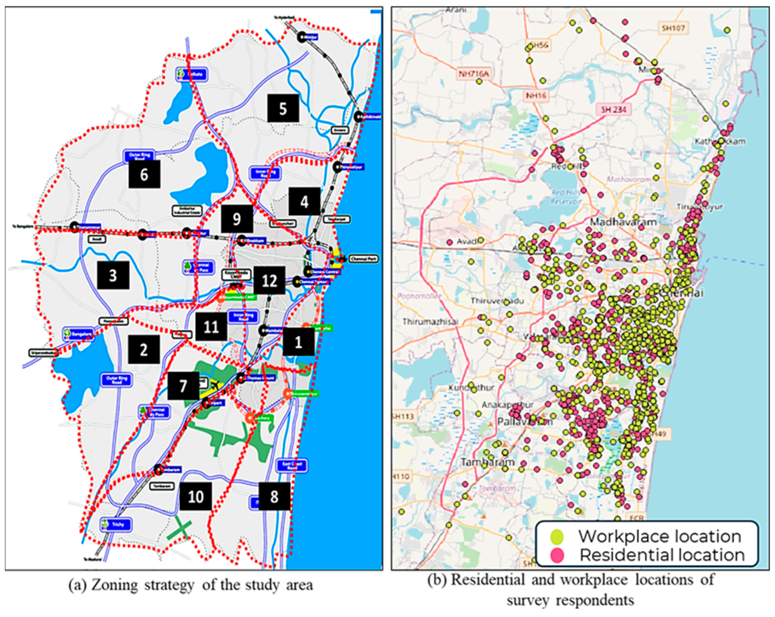
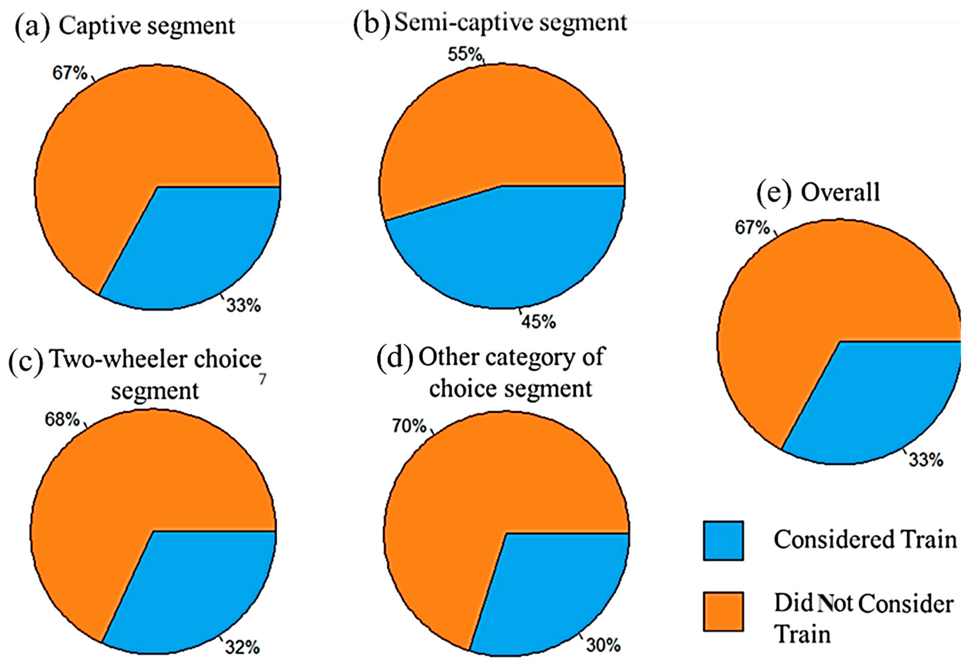
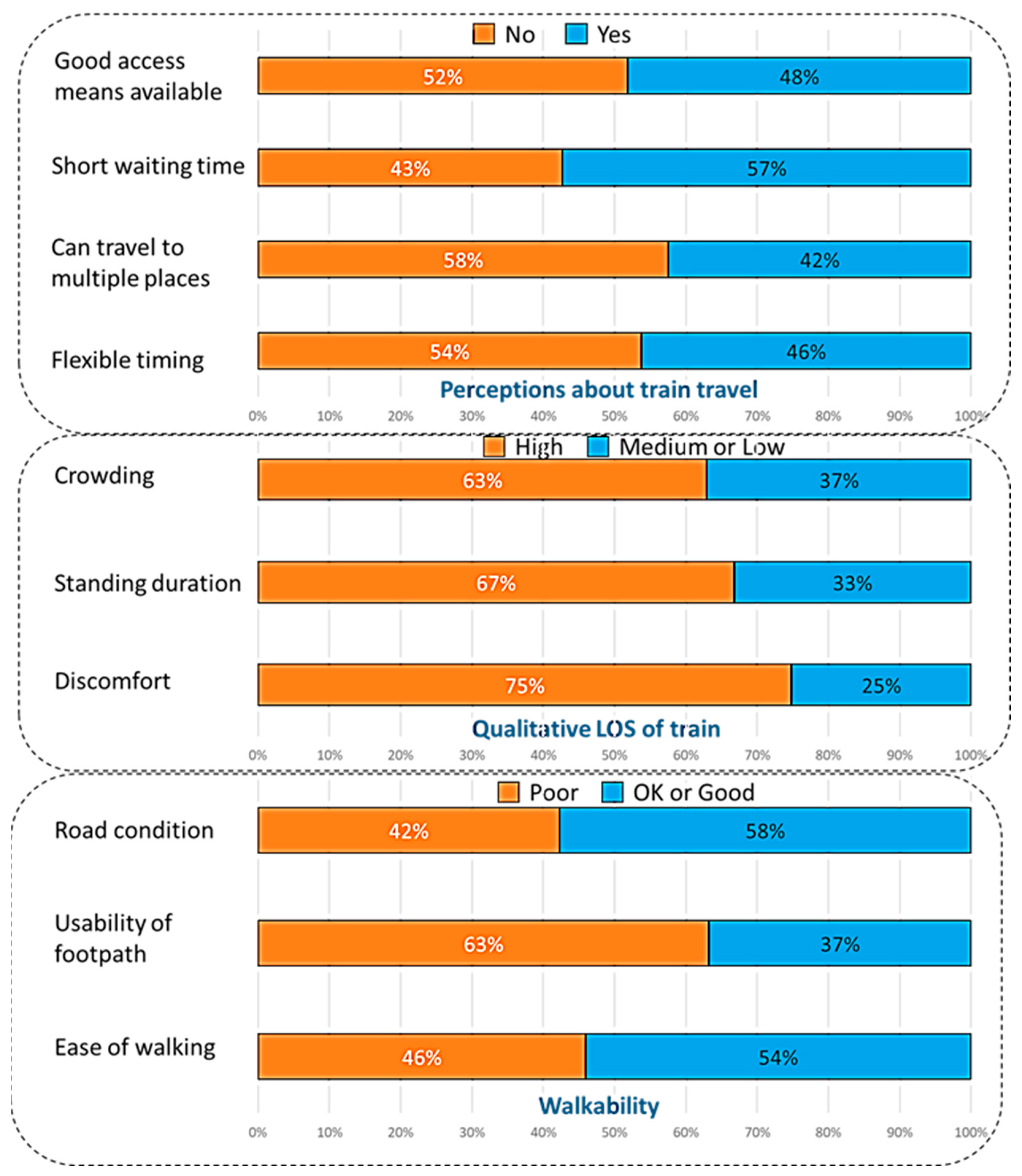
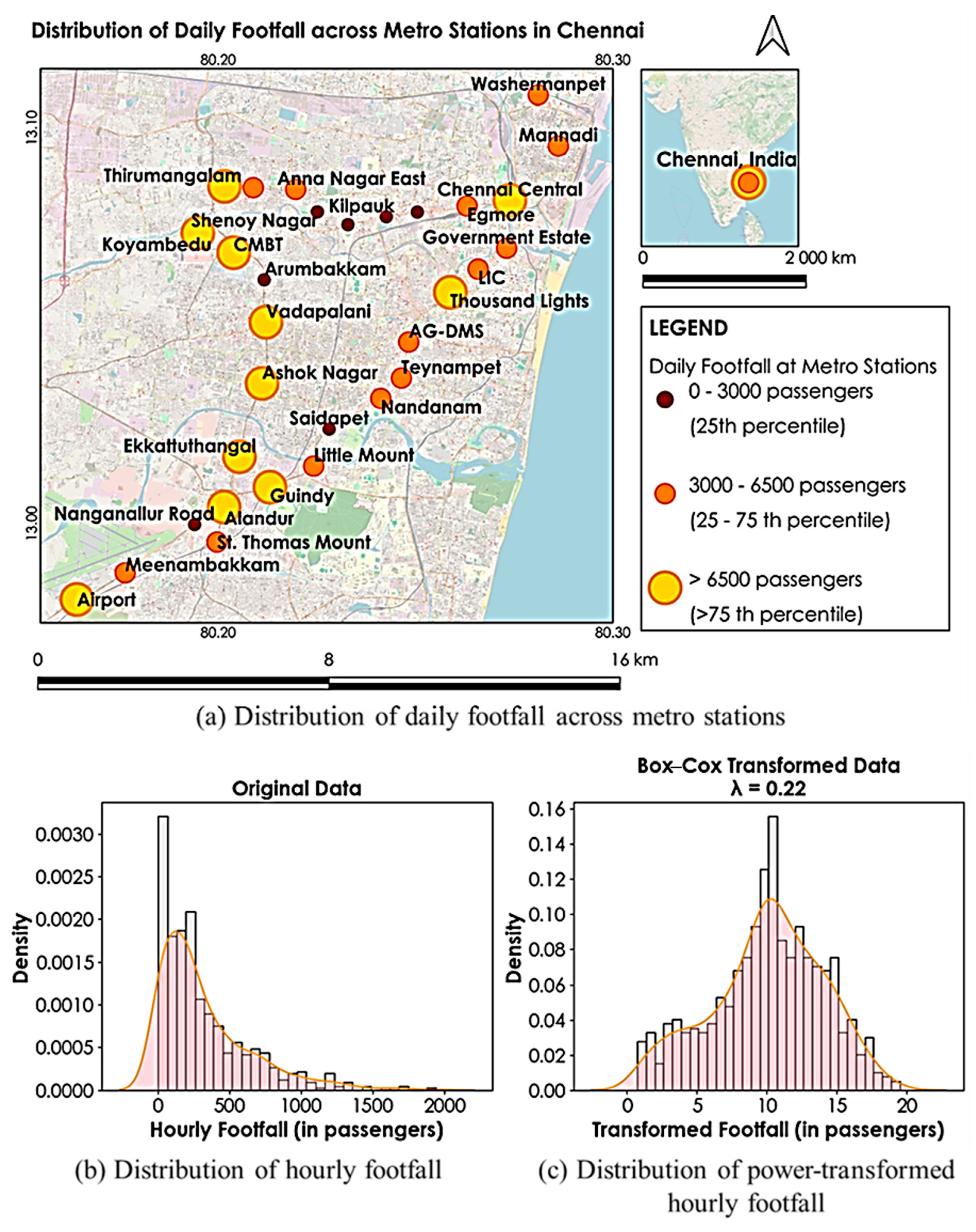
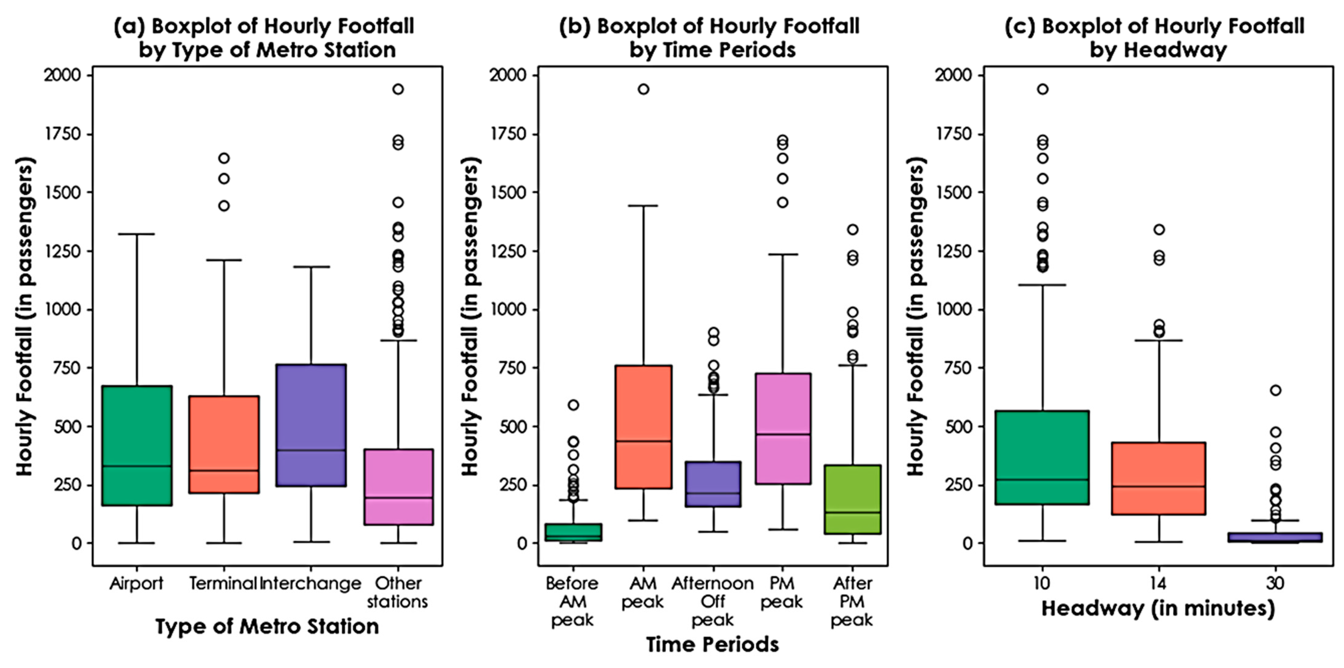

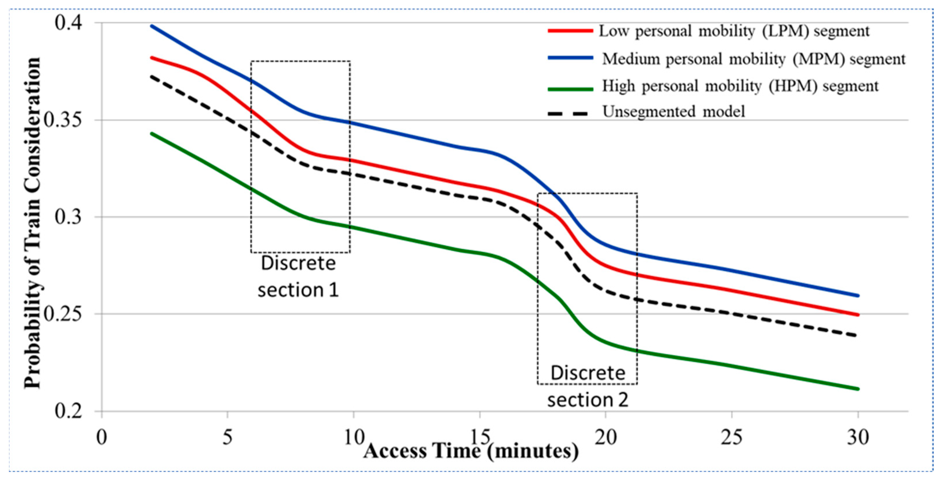
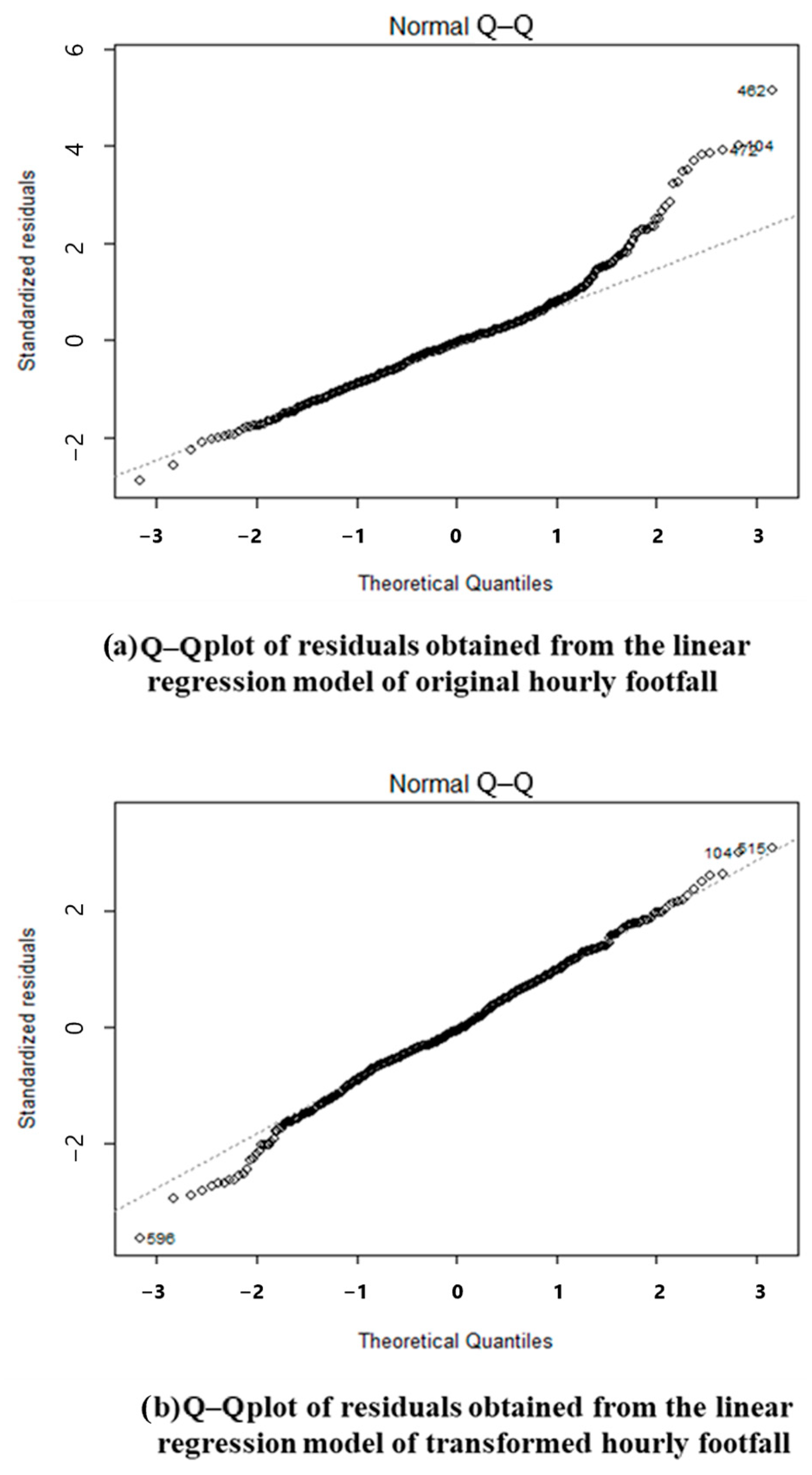
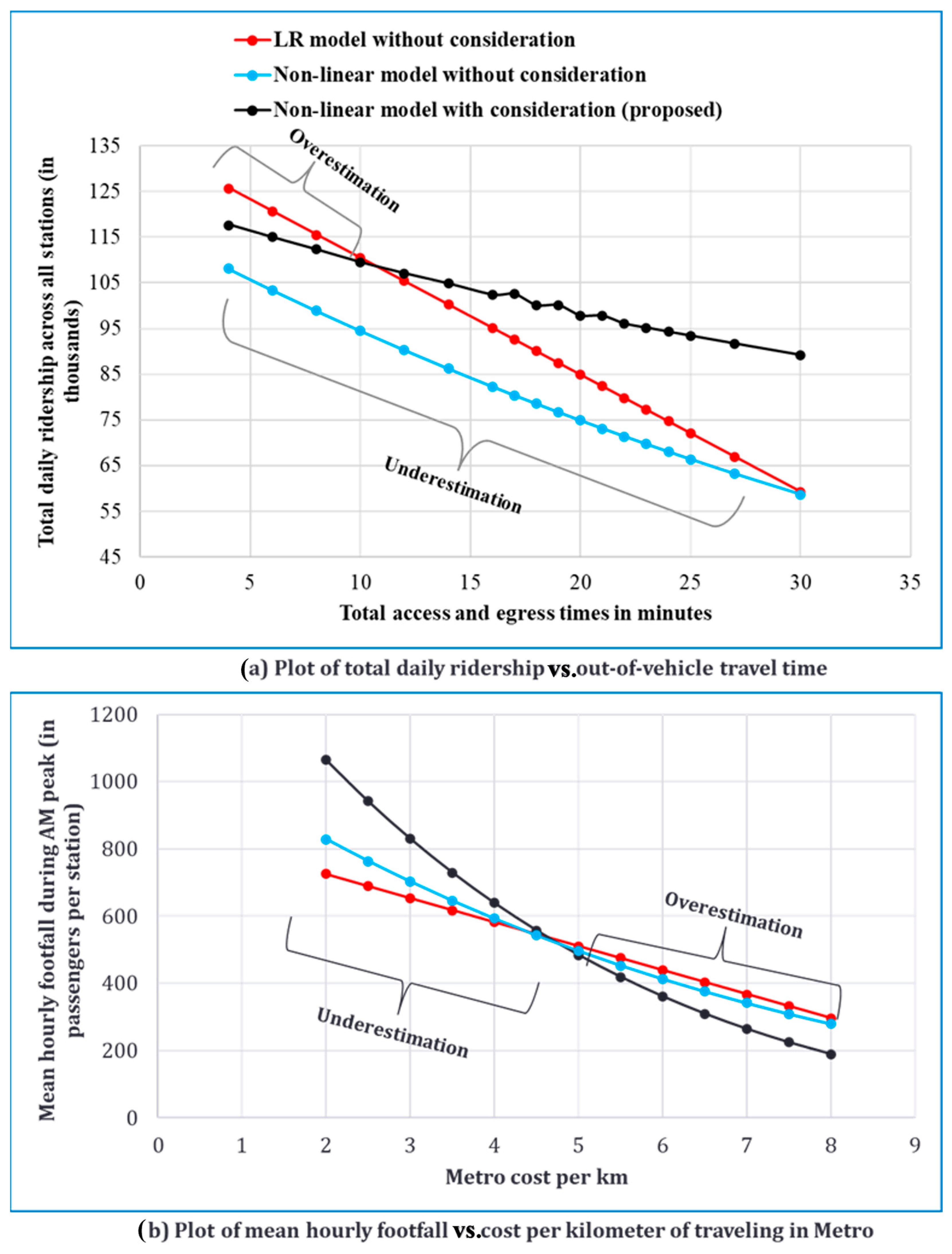
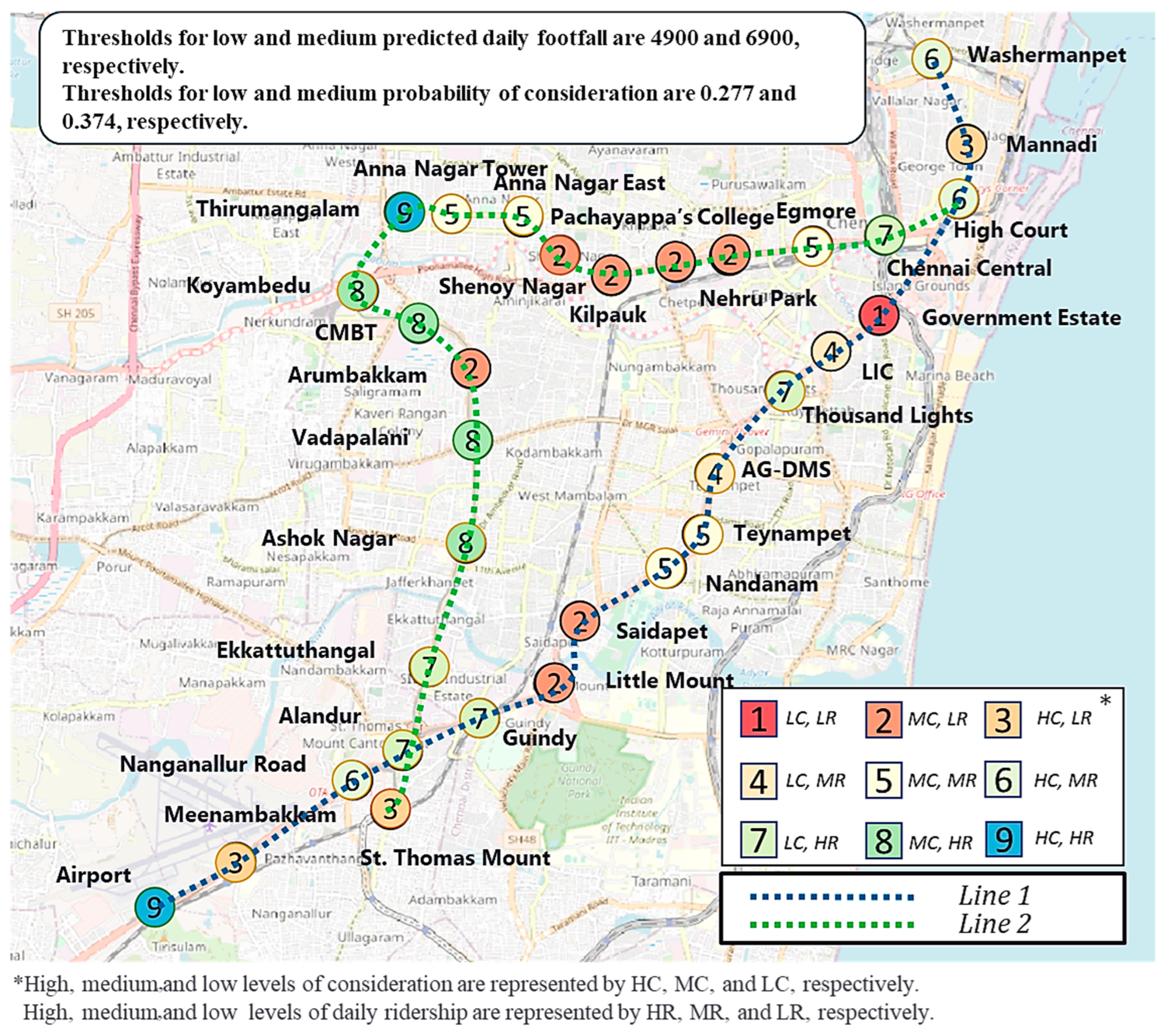
