GAN-Based Generation of Synthetic Data for Vehicle Driving Events

Abstract

Developing solutions to reduce traffic accidents requires experimentation and much data. However, due to confidentiality issues, not all datasets used in previous research are publicly available, and those that are available may be insufficient for research. Building datasets with real data is costly. Given this reality, this paper proposes a procedure to generate synthetic data sequences of driving events using the Time series GAN (TimeGAN) and Real-world time series (RTSGAN) frameworks. First, a 15-feature driving event dataset is constructed with real data, which forms the basis for generating datasets using the two mentioned frameworks. The generated datasets are evaluated using the qualitative metrics PCA and T-SNE, as well as the discriminative and predictive score quantitative metrics defined in TimeGAN. The generated synthetic data are then used in an unsupervised algorithm to identify clusters representing vehicle crash risk levels. Next, the generated data are used in a supervised classification algorithm to predict risk level categories. Comparison results between the data generated by TimeGAN and RTSGAN show that the data generated by RTSGAN achieve better scores than the the data generated with TimeGAN. On the other hand, we demonstrate that the use of datasets trained with synthetic data to train a supervised classification model for predicting the level of accident risk can obtain accuracy comparable to that of models that use datasets with only real data in their training, proving the usefulness of the generated data.

1. Introduction

Access to adequate data is one of the most critical elements in developing machine learning solutions for domain-specific problems [1]. In practice, the benefits of data-driven studies are restricted to the owners of such data [2]. For this reason, it is challenging to conduct research with high accuracy without data availability. The most promising technique in the absence of private data publication is the synthetic data generation approach, where new data sharing the same distribution as the original data are generated. Given that both the original and the synthetic data come from the same distribution, all the queries performed on the synthetic data provide similar results to those obtained from the real data alone [3]. Data generated in artificial modes can complement or create imputations for missing data. Consequently, analysis and evaluation algorithms often rely on synthetic data to test systems in specific dimensions and scenarios [4].

Developing solutions to lowering traffic accidents requires much experimentation, and consequently much data. However, only a few datasets with driving event data are available. Considering this reality, the current project uses Generative Adversarial Networks (GANs) to generate synthetic data. This kind of data can be shared with no risk of exposing confidential information about individuals or entities related to these data. Synthetic data can be used to fill out an initial dataset with driving data gathered from heterogeneous sources. Qualitative and quantitative methods are employed to assess the synthetic data generation results and establish their usefulness.

The main objective of this research is to generate synthetic data using GAN-based frameworks for synthetic time series data and subsequently use the data in tasks to train prediction models for classifying the risk level of certain ways of driving vehicles. The data generated are obtained from a dataset with real information, which is made available to the general public in this work. A dataset with real information provides an answer to the lack of adequate datasets for study. The set of data generated in this research is used in processes to predict the level of risk of accidents in vehicles.

Although publicly available datasets exist, they do not incorporate data from vehicle sensors, drivers, and the environment into the same dataset. In addition, these datasets correspond to countries with realities that are different from that of Ecuador in aspects such as road geometry, road signs, and driving culture, meaning that they are not immediately applicable to local research. Although the code for the TimeGAN and RTSGAN frameworks is publicly available, the datasets on which they are based are not related to vehicle driving events, meaning that the distributions in the data respond to other realities; as a result, the hyperparameters published in the papers presenting these frameworks are not directly applicable to vehicle driving event-related datasets.

The scientific contributions of this article are as follows:

(1)

An initial multidimensional dataset of driving events is constructed with real data from heterogeneous sources, then used to generate synthetic data.

(2)

A solution is developed to generate synthetic data sequences of driving events using the Time-series GAN (TimeGAN) and Real-world time series (RTSGAN) frameworks as well as to configure their hyperparameters.

(3)

A comprehensive comparison of the data generated by both the TimeGAN and RTSGAN frameworks is presented. This comparison was carried out quantitatively using the discriminative and predictive scores established in TimeGAN and qualitatively using the PCA and T-SNE techniques.

(4)

A demonstration of the practical effectiveness of the generated synthetic data is shown by using the data in supervised classification processes with the MLP algorithm to assign a level of accident risk to an event using driving event information. The accuracy obtained by the models using only real data is compared to the accuracy of models using both real and synthetic data.

1.1. Theoretical Background

This section explains the operation of Long Short-Term Memory (LSTM) networks, Generative Adversarial Networks (GANs), and the Time-series GAN (TimeGAN) and Real-world time series GAN (RTSGAN) frameworks used in this paper for data generation.

1.1.1. Long Short-Term Memory Networks

LSTM networks were first introduced by Hochreiter and Schmidhuber in 1997. LSTM is a type of RNN that solves the short memory problem of traditional recurrent neural networks, which are bad at retaining long-term information. LSTM networks can remember information for long periods. In Figure 1, the general architecture of an LSTM cell is depicted, where the gates and the cell state stand out as its most important elements. A gate has a feed-forward layer, followed by a sigmoid activation function and then a pointwise multiplication step. An activation function transforms the vector before computing the loss calculation. The cell state is the memory unit of the network. It is used to encode dependencies and long-term relationships through gates. Each LSTM cell has three inputs, $x_t$, $h_{t-1}$, and $c_{t-1}$, respectively representing the input at time t, the previous hidden state, and the previous cell state, along with two outputs $h_t$ and $c_t$, respectively representing the current hidden state and current cell state [5].

Figure 1. Architecture of an LSTM cell.

1.1.2. Generative Adversarial Networks

A promising approach in synthetic data generation is provided by Generative Adversarial Networks (GANs). Goodfellow et al. [6] were the first to introduce the GAN as a framework for estimating generative models through an adversarial process between the two essential components of a GAN, namely, the generative model or generator network, and the discriminative model or discriminator network. In the beginning, GANs showed successful results for the generation of artificial images; subsequently, they have been proven to perform well with other types of data as well, including electronic health records [1], natural language processing [7], speech enhancement [8], fault diagnosis under imbalanced data conditions [9], imputing missing values [10], and more. In the most outstanding approaches, the neural networks representing the generator and discriminator are typically implemented by a variant of RNN [2].

1.1.3. Time-Series GAN (TimeGAN)

GANs were not created specifically for time series data; they are mainly used with images, and as such do not perform well regarding specific time series properties. The TimeGAN framework was introduced by Yoon et al. [11] in 2019. It seeks to overcome these limitations when generating synthetic data sequences based on a real dataset.

The TimeGAN architecture combines an adversarial network (generator and discriminator networks) with an autoencoder (embedding network and retrieval network). An autoencoder is a neural network that learns a representation of the data in an unsupervised manner and aims to learn an encoding of a dataset by training the network to ignore the noisy signal. Specifically, TimeGAN comprises two groups of networks: (1) encoding networks and (2) adversarial networks. In addition to these network groups, there is another component called the supervisor network. Each network is implemented through a Gated Recurrent Unit (GRU) or LSTM-type RNN network, which receives a three-dimensional tensor as input. A tensor is a type of data structure that can be understood as a multidimensional array [12].

Encoding networks encompass two networks: the embedding network, which acts as an encoder that converts the real data into a latent representation, and the recovery network, which converts the latent representation present in the latent space into reconstructed data. Adversarial networks also include two networks: a (sequence) generator network and a (sequence) discriminator network. The generator network receives a noisy input and produces an output in the latent space (not the feature space); its objective is to learn a distribution $\tilde{p}\left(x_{1:T}\right)$ that approximates the distribution used to generate the actual data $p\left(x_{1:T}\right)$, where $x_{1:T}=x_1,x_2,\cdots ,x_T$ is a multivariate sequence of length T. On the other hand, the discriminator network receives an input from the latent space, then classifies the data as real or synthetic. Lastly, the supervisor network generates a new sequence given a previous series in the latent space H, allowing the quality of the generated sequences to be controlled.

TimeGAN simultaneously learns to encode features, generate representations, and iterate over time. The generator and discriminator networks operate in a latent space provided by the embedding network. The latent and real data dynamics are synchronized through the supervised loss. The four networks comprising the TimeGAN framework and their respective losses are shown in Figure 2.

Figure 2. TimeGAN framework.

TimeGAN considers the contribution of three loss functions: reconstruction, unsupervised, and supervised. These allow for learning of the distribution of the data both at the level of each feature and at the temporal level. The reconstruction loss ensures that data are efficiently encoded and decoded in and from the latent space. The unsupervised loss is produced between the generator and the discriminator network, which forces the generator to create realistic data sequences. The supervised loss allows for generating the next time step in latent space. The generator is trained to ensure that the generator learns the temporal dynamics of the data series, forcing the generator to create realistic data sequences. The supervised loss is also applied to the embedding network in order to preserve the temporal variation used to encode the real sequences.

The TimeGAN algorithm learns in three training phases. First, in the embedding phase, only the embedding and retrieval networks are trained. Next, in the supervised phase, the generator is trained only with supervised loss. Finally, in the joint phase, the algorithm learns to encode, iterate, and generate time series data. All phases are trained over the same number of iterations, as all phases have equal weighting in the original TimeGAN implementation.

The authors of TimeGAN used three metrics as criteria to evaluate the generated data: (1) fidelity, (2) diversity, and (3) usefulness [11]. The fidelity metric indicates that the sample series should be indistinguishable from the real data. The diversity metric refers to the requirement that the distribution of the synthetic data should be similar to that of the real data. Finally, the usefulness metric means that the synthetic data should be as useful as the real data for solving predictive tasks. Figure 3 summarizes these three evaluation criteria.

Figure 3. TimeGAN evaluation scheme.

Fidelity evaluation. This evaluation uses a quantitative metric called the discriminative score. The discriminative score is obtained through a classification model trained with a discriminative LSTM network; its value expresses the ability of the model to identify whether a data sample corresponds to real or synthetic data. A lower score is better, as it means that the discrimination model does not distinguish synthetic from real data very well. The worst possible result is 0.50 and the best is 0.00. The value of this score is provided by Equation (1):

$$\mathit{discriminative} \mathit{score}=\mathit{accuracy}-0.5$$

(1)

which can also be expressed as shown in Equation (2):

$$\mathit{discriminative} \mathit{score}={\displaystyle \frac{\mathit{No}.\mathit{of}\mathit{correct}\mathit{predictions}}{\mathit{Total}\mathit{number}\mathit{of}\mathit{predictions}}}-0.5.$$

(2)

Diversity evaluation. Although there is no direct visual way to assess the appropriateness of synthetic data, the PCA and T-SNE techniques can be used as qualitative assessment metrics. PCA is an algorithm that finds a set of principal components that are orthogonal to each other, where each component captures the largest variance of the data after accounting for the variance accounted for by the previous components. On the other hand, T-SNE is a nonlinear approach that reduces the dimensionality of the data, seeking to maintain the closeness between the points of the original dimensions in the lower dimensional representation. T-SNE uses a T-distribution to represent the probabilities in the lower-dimensional space. This process is the opposite of that used by PCA, which seeks to obtain the highest variance [13]. Both of these methods follow the expectation that the two-component scatter plots of the synthetically generated and the original points should be as similar as possible. These plots provides a visual representation showing whether the distribution of the generated data maintains similar characteristics to the original data distribution.

Usefulness evaluation. The usefulness of synthetic data is measured through a predictive score obtained through a prediction model trained using an LSTM network. Its value expresses the ability of the model to predict the value of one dimension from a multidimensional sequence of data. A value closer to zero reflects better predictive capability on the part of the model. The value of the predictive score is the Mean Absolute Error (MAE), defined by Equation (3)

$$MAE={\displaystyle \frac{1}{n}}\sum _{i=1}^n|x_i-y_i|,$$

(3)

where:

-

$x_i$ represents the actual value for the dimension of the dataset’s i-th sequence.

-

$y_i$ represents the predicted value for the dimension of the dataset’s i-th sequence.

-

n represents the total number of sequences in the dataset.

1.1.4. Real-World Time Series GAN (RTSGAN)

RTSGAN is a framework proposed by Pei [14] that allows for the generation of multidimensional time series data. The RTSGAN architecture has two main components: (1) an encoder–decoder module, and (2) a generator module. Their schematics can be seen in Figure 4. The encoder–decoder (autoencoder) module learns to encode each time series instance into a fixed-dimensional latent vector, from which the time series is reconstructed. The generator module uses a Wasserstein GAN (WGAN) to produce vectors in the same latent space as the autoencoder. The time series are generated by feeding latent synthetic vectors produced in the generator into the decoder.

Figure 4. RTSGAN framework.

The RTSGAN encoder encodes each data series into a compact invariant representation of the sequence length. First, the global y features are concatenated with the dynamic features x in each timestep as ${\mathrm{e}}_i=\left[x_i,y\right]$. These are fed into an N-layer GRU network with $d_{AE}$ hidden dimensions to obtain the states $h_i^N$ at each timestep i at each GRU layer n, as follows:

$${\mathrm{h}}_t^n=\mathrm{GRU}\left({\mathrm{e}}_i\right),i\in \left[1,l\right],n\in \left[1,N\right].$$

(4)

To better capture the temporal dynamics and global properties, pooling operations are applied to the hidden states of the last layer of the GRU network:

$$\mathrm{s}=\mathrm{FC}\left(\left[\mathrm{AvgPool}\left({\mathrm{h}}_i^N\right),\mathrm{MaxPool}\left({\mathrm{h}}_i^N\right),{\mathrm{h}}_l^N\right]\right)$$

(5)

where FC stands for fully connected layer. At the end, the global information $\mathrm{s}$ is concatenated with the last hidden state to obtain a latent representation $\mathrm{r}\in {\mathbb{R}}^{(n+1)d_{AE}}$ for the time series, as follows:

$$\mathrm{r}=\left[\mathrm{s},{\left\{{\mathrm{h}}_l^n\right\}}_{n=1}^N\right].$$

(6)

The RTSGAN decoder attempts to reconstruct the time series from the latent representation r in two steps: (1) reconstruction of the global features $\widehat{\mathrm{y}}$, and (2) reconstruction of the dynamic features ${\mathrm{h}}_l^n$. The global features $\widehat{\mathrm{y}}$ are reconstructed with

$$\widehat{\mathrm{y}}=\mathrm{Act}({\mathrm{W}}_y\mathrm{s}+{\mathrm{b}}_y),$$

(7)

where $\mathrm{Act}$ represents a softmax function for categorical features and a sigmoid function for continuous features.

The dynamic feature decoder is another N-layer GRU network with hidden dimension $d_{AE}$; it takes ${\mathrm{h}}_l^n$ as the initial state ${\widehat{\mathrm{h}}}_o^n$. The reconstruction process follows the scheme

$${\widehat{\mathrm{e}}}_i=\left[{\mathrm{x}}_{i-1},\mathrm{s}\right],$$

(8)

$${\widehat{\mathrm{h}}}_i^n=\mathrm{GRU}({\widehat{\mathrm{e}}}_{\mathrm{i}},{\widehat{\mathrm{h}}}_{\mathrm{i}-1}^{\mathrm{n}}),n\in \left[1,N\right],$$

(9)

$${\widehat{\mathrm{x}}}_i=\mathrm{Act}({\mathrm{W}}_x{\widehat{h}}_i^N+{\mathrm{b}}_x).$$

(10)

The RTSGAN generator uses a version of WGAN. With the help of a 1-Lipschitz discriminator, the generator tries to minimize the 1-Wasserstein distance $W(Pr,Pg)$ between the real data distribution and the synthetic data distribution:

$$\underset{G}{min}\underset{D}{max}{E}_{\mathrm{r}\sim encoder(\mathrm{X},\mathrm{y})}\left[D\left(r\right)\right]-E_{\mathrm{z}\sim p\left(\mathrm{z}\right)}\left[D\left(G\right(\mathrm{z}\left)\right)\right]$$

(11)

where G and D represent the generator and the 1-Lipschitz discriminator, respectively. After training the WGAN, time series are generated as follows:

$$\widehat{\mathrm{X}},\widehat{\mathrm{y}}=\mathrm{decoder}\left(G\left(z\right)\right),z\sim p\left(\mathrm{z}\right).$$

(12)

The code used in this research for data generation with RTSGAN is available at https://github.com/acphile/RTSGAN (accessed on 3 October 2024).

1.2. Related Works

Considering the success of GANs in generating high-quality artificial images, several proposals have focused on generating time series using GANs. Common to these approaches is the need to model data variation over time. One of the drawbacks of vanilla GANs in time series data generation is the instability of the discriminator during training, which can lead to the generator producing only a limited number of outputs.

In the papers from the last five years reviewed as part of this research, a common approach to generating synthetic time series data is to use RNN networks within the generator and discriminator of the GAN network. However, vanilla RNN networks present vanishing gradient or exploding gradient problems. In order to overcome this drawback, in most cases variants of RNN, GRU [9,15,16,17,18], or LSTM [1,2,4,7,8,19,20,21,22,23,24,25,26,27] are used. Other types of networks used in the generation of time series data include Wasserstein GANs [28,29,30], Convolutional Neural Networks [20,24,29,31,32,33], Mixture Density Networks [19], and transformer networks [9,18]. The transformer architecture is currently the state of the art in neural networks, and is a topic of great interest in the time series data generation field.

In most proposals, the generated data have three or fewer dimensions [2,4,9,16,19,20,21,22,23,24,26,29,30,31,32,33,34]. However, several papers involved the generation of multidimensional data with more than three dimensions [1,7,8,9,15,17,18,25,27,28].

Several authors have also demonstrated the effectiveness of their models in downstream tasks. Most of these used generated data to improve the accuracy of prediction models as compared to results using only real data [2,7,9,16,17,23,24,25,32]. In contrast, other authors have used the generated data in clustering processes [21,33].

Biomedical signals generation is the field in which synthetic time series data are most widely used. Medical signals are generated from electroencephalograms (EEGs), electrocardiograms (ECGs), electromyography (EMG), photoplethysmography (PPG), and intensive care units (ICUs) [1,9,20,22,23,24,29,31,32]. Other types of generated data include data network traffic flows [28], sensory data from personal activities [19], driving trajectories [21], IoT traffic [25], internal measurement unit (IMU) data [7], electric vehicle battery parameters [8], content delivery network (CDN) traffic [4], network and computer system data [2], channel impulse responses (CIR) [26], astronomical light curves [32], power demand [32], highway cut-in behaviors [18], power consumption [15,30,33], solar generation [33], machine fault diagnosis [9], photovoltaic power [16], hydration monitoring [17], and physiological signals and markers [27].

Concerning the generation of vehicle driving data, important works include those of Demetriou et al. [21], who generated data for the longitude and latitude components of driving trajectories; Jaafer et al. [7], who generated data from an IMU (longitudinal acceleration, lateral acceleration, pitch, yaw, and roll) to classify the driving style of portions of trips as normal or aggressive; and Yang et al. [18], who generated data on lane change scenarios on highways. The sequences generated in these works were of short duration (up to 12 s) and the number of dimensions used was small (less than or equal to 5). The technical challenge faced in this research is greater than that of the above works, as it relates to driving event data using multidimensional data with fifteen features and generating sequences of 24 s in duration, resulting in a more robust model. Because of this, the data sequences generated in our work are more realistic, as they capture distributions of greater complexity created by the presence of a greater number of variables for a longer amount of time.

This paper comprises four sections: Section 1 describes the theoretical framework and work related to the generation of synthetic time series data using GANs; Section 2 details the materials and methodology used, and describes the experimental part of this work; Section 3 presents the main results obtained with the synthetically generated data and discusses these results; finally, Section 4 presents our conclusions and prospects for future work.

2. Materials and Methods

This section describes the elements required to perform our experiments, including the materials needed, the essential software, the construction of the dataset, and the setup of the software environment for TimeGAN. It also details the setup for generating synthetic data from the constructed dataset with TimeGAN and RTSGAN, evaluating the resulting data, and demonstrating the usefulness of these data in downstream tasks.

2.1. Materials

The following materials were used to obtain and process the experimental dataset. The main element needed to obtain the data was a car in operation, as certain driving events can be characterized by reading its sensors. Other equipment used to collect the dataset data included a Veepeak OBD-II scan tool, a Huawei Redmi 6A phone with Android 9 PPR1 with the Car Scanner Pro application, and a Core i5-8400 desktop computer with 8 GB of RAM. Regarding the software, Python with TensorFlow 1.15 was used for the data preprocessing scripts, synthetic data generation with TimeGAN, and prediction models, while Python and R were used to create plots and charts.

Dataset Details

This section details the tasks that were performed to build the final dataset used in the experiments, starting from the decision on the size of the dataset through the reading of the data from the vehicle sensors to the data preprocessing tasks.

To estimate the size of the dataset, we considered datasets used in other studies related to the generation of synthetic data. In the work of [19], 7000 timesteps were used in the authors’ proposed artificial data generation model. In [35], the authors used a dataset with 7056 timesteps to compare two data generation models, one based on a GAN and the other of autoregressive type. In [11], a dataset with 3773 stock market records was used. For this work, we built a dataset of 2634 records or timesteps, with each record comprising fifteen attributes or features.

The data in the built real dataset were obtained mainly from the data generated by a vehicle driven by the same person traveling a route for about 50 min. The route crosses Sangolquí-Pifo Avenue and then continues along the Alpachaca Corridor until reaching the Mariscal Sucre International Airport in the Tababela sector; the map of the route can be seen in Figure 5.

Figure 5. Map of the trajectory followed by the vehicle.

All of the collected data received the respective authorizations from the data owners for use in this research through their written consent. These data were read from the vehicle and recorded every second by the Car Scanner Pro app installed on an Android smartphone placed inside the vehicle. This app was connected via Bluetooth to an OBD-II dongle connected to the vehicle’s OBD-II interface. On-Board Diagnostics II is a vehicle diagnostic system that monitors, among others, the emissions, mileage, speed, and temperature of the car; almost all modern light vehicles of American origin manufactured since 1996 incorporate an OBD-II diagnostic port. The ISO-15765-4:2021 standard specifies the communication requirements between the Controlled Area Network (CAN) and the diagnostic system (OBD-II) of a vehicle. The schematic of the interconnection of these components is shown in Figure 6. Depending on the vehicle’s type, equipment, and make, this app can obtain more or less data about the car.

Figure 6. An OBD-II scanner transmits data read from the vehicle via Bluetooth to the Android app.

In addition to the data read from the vehicle, we used a smartwatch to obtain the driver’s biometric data at each instant while driving the car. Data from the external environment were calculated from the Global Positioning System (GPS) location of the vehicle, as well as data from traffic accidents occurring in the vicinity of the sites included along the route traveled by the car.

Although there is no single combination of characteristics that identifies driving behavior, most studies include longitudinal speed [36], acceleration, throttle position, and revolutions per minute (RPM) among their selected characteristics [37]. These and other characteristics were included in our study to classify the level of risk of traffic accidents. A general description, together with the measurement units of each column or feature of the constructed dataset, is provided in Table 1. The visual appearance of the signals of each column can be seen in Figure A1 of the Appendix (Dataset Features Signals section). To complement this information about the dataset, Table 2 shows the code used for each dataset feature along with the minimum, maximum, and average values.

Table 1. Dataset columns description.

No.	Feature	Meaning
1	steering_angle	Angle between the projection of a vehicle’s longitudinal axis and the line of intersection of the wheel plane and the road surface (sexagesimal degrees).
2	speed	Speed of the vehicle in meters per second (m s−1).
3	rpm	Speed of the vehicle engine in revolutions per minute (RPM).
4	acceleration	Acceleration of the vehicle in meters per second squared (m s−2).
5	throttle_position	Sensor used to monitor the air intake of an engine (%).
6	engine_temperature	Temperature of the air entering the engine (°C).
7	system_voltage	Voltage of the vehicle’s electrical system (V).
8	distance_travelled	Distance travelled by the vehicle in one unit of time (km).
9	latitude	Angle between the plane of the earth’s equator and the line perpendicular to the standard spheroid at a given point on the earth’s surface (degrees).
10	longitude	Distance on the earth’s surface east or west of a defined meridian, usually the meridian of Greenwich, England (0° longitude), expressed in angular measurements from 180° west (or −180°) to 180° East (degrees).
11	heart_rate	Number of contractions of the heart per minute.
12	current_weather	Categories for daily weather forecasts for a location (https://developer.accuweather.com/weather-icons) (accessed on 3 October 2024).
13	temperature	Temperature forecast for a specific location (°C).
14	precipitation	Water that falls from the clouds towards the ground (mm).
15	accidents_onsite	Number of accidents recorded within an approximate radius of 100 m around a specific geographic location.

Table 2. Dataset statistics.

No.	Code	Feature	Minimum	Maximum	Average
1	ste	steering_angle	−522.40	515.80	36.13
2	spe	speed	0.00	92.00	49.16
3	rpm	rpm	562	6219	2996.72
4	acc	acceleration	−1.59	2.09	0.18
5	thr	throttle_position	0.00	76.47	25.98
6	eng	engine_temperature	0.00	92.00	83.47
7	vol	system_voltage	0.00	13.00	12.59
8	dis	distance_travelled	0.00	36.33	19.82
9	lat	latitude	−0.33	−0.12	−0.23
10	lon	longitude	−78.43	−78.32	−78.36
11	hea	heart_rate	59.00	77.00	66.32
12	wea	current_weather	6	7	6.38
13	tem	temperature	20.00	24.60	22.80
14	pre	precipitation	0.30	0.50	0.42
15	acd	accidents_onsite	0	42	5.20

The initially constructed dataset of real observations included the nineteen features shown in the matrix in Figure 7.

Figure 7. Initial correlation matrix of features in the constructed dataset.

Due to the high correlation of certain features which had values close to 1, it was necessary to eliminate some of them, as several features conveyed the same information, leading to redundancy, and would make the model training process more complex. It was also important to consider the criteria of other researchers, who suggested retaining some features despite their high correlation. After this process, the matrix in Figure 8 played a crucial role in selecting the features for the final dataset.

Figure 8. Final correlation matrix of features in the constructed dataset.

With the fifteen final dataset features selected, the dataset was preprocessed to (1) fill in missing values, where the value of the closest previous record was used instead of the missing value; (2) encode categorical data, where categorical data were converted to numerical data; and (3) normalize data to ensure an equal contribution of each feature to training the data generation model. It is worth mentioning that data normalization is performed as part of the initial reading of the data in TimeGAN.

2.2. Methodology

This section details the adjustments used to generate synthetic data from the constructed dataset, evaluate the resulting data, and demonstrate their practical utility. The general procedure followed to generate the synthetic data was as follows: (1) the values of the TimeGAN hyperparameters were adjusted; (2) data were generated with TimeGAN using the obtained hyperparameters; (3) the RTSGAN hyperparameters were adapted to make them correspond to the main TimeGAN hyperparameters; (4) data were generated with RTSGAN using the configured hyperparameters; (5) the data obtained with both frameworks were evaluated; and (6) the practical application of the generated data was demonstrated by using them in a prediction model.

This work uses LSTM networks for all TimeGAN neural networks, as they are suitable for learning temporal patterns in long sequences [22]. The initial data were two-dimensional (observations, features). However, to train TimeGAN networks a three-dimensional tensor is required as input in the form (sequences, timesteps, features). TimeGAN performs an internal preprocessing step on the original data to obtain the tensor prior to training.

Equation (13) allows us to obtain the number of sequences to be generated with TimeGAN, which depends on the number of observations in the initial dataset and the sequence length. The number of dimensions is the same for both the number of observations in the initial dataset and the generated sequence data.

$$s=n+l-1$$

(13)

In this equation:

-

s is the total number of observations in the dataset;

-

n is the total number of sequences;

-

l is the length of each sequence.

For example, if a dataset has 2634 observations and the length of the sequences is 24, then the number of sequences to be obtained with Equation (13) is 2611. Thus, the values of the tensor dimensions input to TimeGAN are as shown in Table 3.

Table 3. TimeGAN network input tensors.

Dimension	Dimension Name	Value
1	No. of sequences or samples	2611
2	No. of timesteps per sequence 1	24
3	No. of features per timestep	15

¹ Also known as sequence length.

2.2.1. TimeGAN Implementation

TimeGAN was implemented in Python using the TensorFlow package as a basis in this work. The TensorFlow installation procedure is detailed in https://github.com/laboratorioAI/2023_SyntheticDrivingData/blob/main/Appendices/Installation_and_configuration_of_TensorFlow_1_15.pdf (accessed on 3 October 2024).

2.2.2. TimeGAN Initial Hyperparameters

For this study, almost of all the same hyperparameter values are shared for all TimeGAN networks (including the supervisor network). Table 4 shows the initial values of the main hyperparameters of these networks, which were established on the basis of some of the reviewed works and a preliminary set of experiments.

Table 4. Hyperparameters for initial experiments.

TimeGAN Hyperparameter	Initial Value
Length of the sequence of timesteps 1	24
Module type of the RNNs	LSTM
Hidden units for RNNs 2	80
Layers for the LSTM networks 3,4	3
Batch size 3	128
Iteration	500
Optimizer	ADAM
Learning rate	0.001
Loss function for classification	BCE
Loss function for regression	MSE

¹ The tuning of this hyperparameter is detailed in Appendix B.2. ² The tuning of this hyperparameter is detailed in Appendix B.3. ³ The values for the number of layers and batch size were set to 3 and 128, respectively, as applied in [11]. ⁴ The embedding, recovery, generator, and discriminator networks have three layers. Only the supervisor network has two layers.

2.2.3. TimeGAN Networks Architecture

Figure 9 shows the details of all the inputs and outputs of the LSTM network cells of the TimeGAN networks used in this work. It describes the vertical flow from the input layer to the output layer and the horizontal flow through each timestep of the sequence. In this figure, a sequence is an array of vectors of length s$\{X_1,X_2,\dots ,X_t,\dots X_s\}$ that represents the number of entries to the LSTM network for each batch element. The number of features corresponds to the number of features in the original dataset, which in this work is 15. The number of hidden units is a hyperparameter of each LSTM cell.

Figure 9. Detailed LSTM network.

The LSTM network has three layers, each comprising s LSTM cells. Each LSTM cell receives three inputs: the cell state $c_{t-1}^n$ of the previous timestep of the current layer n, the hidden (output) value $h_{t-1}^n$ of the prior cell of the current layer n, and the current input vector. If the layer is the first one, then the current input is $X_t$; otherwise, the input is the hidden state of the previous layer. Each LSTM cell produces two outputs: (1) the hidden state $h_t$ and (2) the cell state $c_t$. The $h_t$ state constitutes the short-term memory of the network, which is sent to the next cell within the same layer and forms the output of that cell. On the other hand, the state $c_t$ corresponds to the long-term memory of the network, and its use is internal to the network. The array of state vectors $h_t^n$ (outputs of the n layer) is transmitted to the upper layer of the network. In the last layer, this array constitutes the network output, represented by the array of vectors of length s$\{H_1,H_2,\dots H_t,\dots H_s\}$; each of these vectors has D dimensions, which in this case is equal to the number of hidden units of each LSTM cell. The output used in this work for training the networks is the $H_{24}^3$ state, which corresponds to the last timestep of the network’s last layer.

2.2.4. Initial Configuration of Evaluation Networks

The discriminative and predictive scores of the evaluation metrics were obtained using two recurrent LSTM networks called the discriminative and predictive networks, which differ from the TimeGAN LSTM networks used in the synthetic data generation process.

Table 5 shows the number of learnable parameters and the input and output dimensions of the discriminative and predictive networks.

Table 5. Information of the evaluation networks.

Characteristic	Discriminator	Predictor
No. of parameters	616	22,751
Input shape	(24, 15)	(23, 14)
Output shape	1	(23, 1)

The architecture of these networks is similar to the on shown in Figure 9; however, in this case the number of layers for the discriminative network is one and the number of layers for the predictive network is two.

The following configuration was used for training the discriminative network: (1) the datasets of the original data and the synthetic data generated with TimeGAN were divided into two groups each, with 70% of each set assigned to the training data and 30% to the test data; (2) the network was trained with mini-batches of the training datasets; (3) the obtained model was tested using the test data from the original and synthetic data datasets, then the discriminative score was calculated.

For the predictive network, the training was performed with mini-batches formed from the synthetic data generated using TimeGAN. The original data were used to test the obtained model. First, the prediction was made using the original data; this prediction was then compared with the true values to calculate the predictive score.

The initial hyperparameters of discriminative and predictive networks are shown in Table 6. Similarly to the TimeGAN networks, these initial values were established based on some of the reviewed works and a preliminary set of experiments.

Table 6. Initial hyperparameters for the evaluation networks.

Network Hyperparameter	Discriminator	Predictor
Module type	LSTM	LSTM
Number of layers	1	2
Hidden units	7 1	30 2
Batch size	32	32 3
Number of iterations	100	500 3
Dropout rate	0.20	0.20
Optimizer	ADAM	ADAM
Learning rate	0.001	0.001
Loss function	BCE	MAE

¹ This value corresponds to half (rounded down to the nearest integer) of the original dataset’s dimensions. ² This value corresponds to twice the 15 dimensions of the original dataset. ³ This is only an initial value. The tuning of this hyperparameter is detailed in Appendix B.4.

2.2.5. Experimental Setup

The strategy used to generate synthetic data with TimeGAN and RTSGAN was realized in two main phases: (1) determining the values for the hyperparameters of the TimeGAN networks and the discriminative and predictive networks used to evaluate the generated data; and (2) executing experiments to generate synthetic data with TimeGAN and RTSGAN using the hyperparameters defined in the previous step.

Hyperparameter tuning or optimization is the process of choosing a set of hyperparameters that achieve the best performance of a data model within a reasonable budget [38]. Determining the best values for the hyperparameters of TimeGAN is a complex task due to the number of hyperparameter combinations that can be defined. In this paper, we follow a two-step method: (1) defining the range of values that the hyperparameters can take based on TimeGAN values [11], and (2) selecting specific values within that range which are as equally spaced from each other as possible. We carried out experiments to determine the hyperparameter values for three types of networks: (1) TimeGAN, (2) discriminative network, and (3) predictive network. This process included the execution of the following three series of experiments:

• The first series obtained a set of candidate values for the hyperparameters of the discriminative and predictive networks.
• The second series obtained the final values of the hyperparameters of the TimeGAN networks.
• The third series adjusted the final values of the hyperparameters of the discriminative and predictive networks using the candidate values obtained in the first series of experiments, then used these networks to evaluate the data generated with the TimeGAN configuration defined in the second series of experiments.

2.2.6. Candidate Hyperparameters for the Evaluation Networks

A first set of experiments was run to generate data with TimeGAN using the initial configuration of hyperparameters (number of iterations, sequence length, and number of hidden units) defined in Table 4. The generated data were then evaluated using the discriminative and predictive networks with the initial hyperparameters shown in Table 6. These experiments used 100, 200, 250, 500, 1000, and 2000 iterations for the discriminative network and 500, 1000, 2000, 4000, 5000, and 8000 iterations for the predictive network. The details of these experiments are provided in Appendix B.1. As a result of these experiments, the best candidate values for batch size and number of iterations were 32 and 200 for the discriminative network and 256 and 500 for the predictive network, respectively.

2.2.7. TimeGAN Hyperparameters

A second set of experiments was performed in which synthetic data were generated with TimeGAN over 500, 3000, 5000, 9000, 10,000, 15,000, 20,000, 25,000, and 30,000 iterations using the values obtained hyperparameters of the TimeGAN evaluation networks in the previous step. These experiments are described in Appendix B.5. As a result of these experiments, the hyperparameter values of 24 for the sequence length and 80 for the number of hidden units were selected for the TimeGAN networks.

2.2.8. Final Hyperparameters of Evaluation Networks

A third and final round of experiments was run to generate data with TimeGAN over 500, 3000, 5000, 9000, 10,000, 15,000, 20,000, 25,000, and 30,000 iterations, with the following results: (1) the best number of iterations to generate data with TimeGAN was 10,000; (2) the most appropriate number of iterations for the predictive network was 8000; and (3) the best batch size for the predictive network was 512. The details of these experiments are provided in Appendix B.4.

2.2.9. TimeGAN Data Generation

Table 7 and Table 8 show the final values of the hyperparameters used in the third round of experiments discussed in Section 2.2.8. Three experiments were run with these hyperparameters to generate data, then the discriminative and predictive score values were averaged to obtain the values reported in the results.

Table 7. Final TimeGAN hyperparameters.

TimeGAN Hyperparameter	Final Value
Length of the sequence of timesteps	24
Module type of the RNNs	LSTM
Hidden units for RNNs	70 1
Layers for the LSTM networks 2	3
Number of iterations	10,000
Batch size	128
Optimizer	ADAM
Learning rate	0.001
Loss function for classification	BCE
Loss function for regression	MSE

¹ The derivation of these values is detailed in Appendix B.5. ² The supervisor network has only two layers.

Table 8. Final hyperparameters for TimeGAN evaluation networks.

Network Hyperparameter	Discriminator	Predictor
Module type	LSTM	LSTM
Number of layers	1	2
Hidden units	7	30
Batch size	32	512
Number of iterations	200	8000
Dropout rate	0.20	0.20
Optimizer	ADAM	ADAM
Learning rate	0.001	0.001
Loss function	BCE	MAE

2.2.10. RTSGAN Data Generation

The final values shown in Table 9 were used for data generation with RTSGAN. Three experiments were run with these hyperparameters to generate data, then the discriminative and predictive score values were averaged to obtain the values reported in the results.

Table 9. Final RTSGAN hyperparameters.

RTSGAN Hyperparameter	Final Value
Length of the sequence of timesteps	24
Module type of the RNNs	GRU
Hidden units for RNNs	70
Layers for the GRU networks	3
Number of epochs 1	2000
Number of iterations	10,000
Batch size	128
Discriminator updates per generator update	2
Learning rate	0.001

¹ The derivation of this value is detailed in the Appendix (Determination of the Number of Epochs Hyperparameter section).

2.2.11. Evaluation of Data Generated with TimeGAN and RTSGAN

The evaluation scheme of TimeGAN proposed by [11] comprises evaluation of the fidelity, diversity, and usefulness of the generated data. These criteria are described in Section 1.1.3.

The fidelity and usefulness of the generated data are expressed by the discriminative and predictive scores, respectively, that is, the discriminative and predictive scores respectively express the fidelity and usefulness of the generated data. The values of these scores were compared between the TimeGAN and RTSGAN frameworks.

The evaluation was carried out using PCA and T-SNE plots in two dimensions. These plots were produced for all experiments in the final round. The PCA and T-SNE plots use different colors to indicate the points corresponding to real or synthetic data. The higher the overlap of both types of points, the better the quality of the generated data. Figure 10 and Figure 11 show the changes in the PCA and T-SNE plots when running different numbers of iterations.

Figure 10. Evolution of the quality of PCA plots.

Figure 11. Evolution of the quality of T-SNE plots.

It can be seen in Figure 10 that the PCA plots in subfigures (a), (b), (h), and (i) show zones with high concentrations of points for the synthetic data distribution, while subfigures (c), (d), (e), (f), and (g) show a better spread of points along the whole plot. As a general rule, plots with a similar distribution of real and synthetic points indicate better ability of the model to generate data over the entire range of real data. Subfigure (e) shows the plot of the model that obtains the best results in TimeGAN with 10,000 iterations. A good overlapping data distribution can be perceived in this plot.

For the T-SNE plots, the optimized hyperparameters shown in Table 10 were used.

Table 10. T-SNE hyperparameters.

T-SNE Hyperparameter	Value
No. of components	2
Perplexity	40
No. of iterations	3000
Learning rate	170

In the case of the T-SNE plots, it can be observed in Figure 11 that the synthetic data form clusters with high point density in subfigures (a), (g), (h), and (i), while in subfigures (b), (c), (d), (e), and (f) the real and synthetic data overlap without forming clusters.

In subfigure (e) of Figure 11, corresponding to 10,000 iterations, the synthetic data overlap with the real data in almost all zones, which is consistent with the PCA results.

2.2.12. Application of Synthetic Data

In addition to the two ways of evaluating synthetic data indicated above, two forms of using synthetic data were applied in order to compare their usefulness against real data through an unsupervised algorithm (clustering) and a supervised algorithm (classification). The synthetic data generated in the experiments were used to build classification models to identify vehicle accident risk levels based on information from driving events, driver biometric data, and the external environment.

Figure 12 shows the two-step practical application scheme of the data generated with TimeGAN. First, the generated data were labeled with the help of a clustering algorithm; then, a supervised prediction algorithm was used to train a classification model.

Figure 12. Synthetic data application scheme.

2.2.13. Clustering Model

Because neither the real data nor the synthetic data generated with TimeGAN have any labels in their records that would allow for identifying the classes or levels of risk of suffering an accident, it is necessary to somehow identify these classes. For this purpose, the K-means unsupervised clustering algorithm was applied to the dataset, using the result provided by the Elbow method as the optimal number of clusters. The number of clusters obtained with this algorithm corresponds to the number of classes. The number of classes identified in the real and synthetic datasets is expected to be the same, as this indicates that the synthetic data are similar to the real data. The Elbow method was applied to one dataset consisting of real data and another dataset consisting of synthetic data. In both cases, 2634 points were used.

The Elbow method obtains a graph that relates the number of clusters to the inertia variation as the result. The inertia measures the total sum of the squares of the distances from each point to the centroid of its respective cluster. The optimal number of clusters corresponds to the point on the graph from which the variation in the inertia is much smaller than that of the previous points. Figure 13 shows that the Elbow method indicates the same number of clusters (four) for both the real and synthetic data.

Figure 13. Identification of the number of clusters with the Elbow method.

After using the clustering process to define the optimal number of classes present in both datasets as four, the next step was data labeling, in which each class was identified with a name. The names assigned to the four classes representing the driving risk level were (1) Very High, (2) High, (3) Medium, and (4) Low. The cluster to which each point belonged was then identified using the K-means algorithm with k equal to 4. In addition to the opinions of our researchers based on their experience, the decision to label the four clusters identified as Low, Medium, High, and Very High Risk was supported by the work of [39], who related several pairs of driving event features and then identified high accident risk clusters, as well as by [36], who used a semi-supervised approach to classify driving styles as either normal or aggressive.

2.2.14. Classification Models

After the real and synthetic data datasets were labeled, the next step was to use the data to create predictive models. We followed a strategy of training several classification models with the supervised learning Multi-Layer Perceptron (MLP) algorithm, then obtaining the accuracy metric corresponding to each model. Table 11 shows the configuration used for the MLP algorithm.

Table 11. MLP configuration.

MLP Hyperparameter	Value
No. of layers	3
First layer units	10
Second layer units	10
Third layer units	10
No. of iterations	10,000
Activation function	ReLU
Solver	ADAM
Learning rate	0.001

The following two experiments were run with TimeGAN-generated data:

• A dataset with 2634 real observations was used for training and testing with holdout-type validation (80–20%).
• A dataset of 2634 records consisting entirely of synthetic data was used for training and a dataset of 2634 real observations was used for testing, applying the Train on Synthetic Test on Real (TSTR) approach.

3. Results and Discussion

This chapter describes the data obtained with the TimeGAN model. In addition, the results obtained in the experimental part are shown and discussed with respect to the evaluation shown in Figure 3 for the data generated with TimeGAN under the criteria of fidelity, diversity, and usefulness.

3.1. Quantitative Evaluation of the Generated Data

As shown in Figure 3, the quantitative metrics in TimeGAN evaluate the fidelity of the data generated through a discriminative score and the usefulness of the data through a predictive score. To obtain these scores, experiments were carried out with the final hyperparameters shown in Table 7 and Table 8 for TimeGAN and Table 9 for RTSGAN. Table 12 shows the scores obtained for the data generated with TimeGAN, while Table 13 shows these scores for the data generated with RTSGAN. A comparison of the scores obtained with TimeGAN and RTSGAn is shown in Table 14.

Table 12. Quantitative evaluation of data generated with TimeGAN.

Number of Experiment	Discriminative Score	Predictive Score
1	0.045663	0.044151
2	0.045918	0.047563
3	0.046492	0.046468
midrange	0.046078	0.045857

Table 13. Quantitative evaluation of data generated with RTSGAN.

Number of Experiment	Discriminative Score	Predictive Score
1	0.017793	0.041440
2	0.018622	0.041782
3	0.021301	0.042283
midrange	0.019547	0.041862

Table 14. Comparison of quantitative metrics between TimeGAN and RTSGAN.

	Type of Framework for Time Series Generation
Metric	TimeGAN 1	RTSGAN 2
Discriminative score	0.046078 ± 0.000415	0.019547 ± 0.001754
Predictive score	0.045857 ± 0.001706	0.041862 ± 0.000422

¹ The values reported here correspond to the midrange values of the results shown in Table 12. ² The values reported here correspond to the midrange values of the results shown in Table 13.

Table 13 shows the discriminative and predictive scores for the data generated with the final values of the RTSGAN hyperparameters, shown in Table 9.

3.2. Qualitative Evaluation of the Generated Data

The qualitative metrics in TimeGAN evaluate the diversity of the data generated. These metrics correspond to the plots generated with the PCA and T-SNE techniques. These plots were created with the data generated in the experiments indicated in Table 12 and Table 13, corresponding to TimeGAN and RTSGAN, respectively. The PCA plots obtained for TimeGAN and RTSGAN are shown together in Figure 14, while the T-SNE plots obtained for TimeGAN and RTSGAN are shown together in Figure 15.

Figure 14. PCA plots obtained with TimeGAN and RTSGAn for 10,000 iterations.

Figure 15. T-SNE plots obtained with TimeGAN and RTSGAN for 10,000 iterations.

Figure 14 and Figure 15 show that the data generated with RTSGAN present a more homogeneous distribution than the data generated with TimeGAN compared to the original data distribution.

3.3. Generated Data Samples

Table 15 and Table 16 show part of a synthetic data sequence obtained with the developed models for TimeGAN and RTSGAN, respectively. The table headers’ row abbreviations correspond to the features listed in Table 2.

Table 15. Data sample generated with TimeGAN.

ste a	spe	rpm	acc	thr	eng	vol	dis	lat	lon	hea b	wea c	tem	pre	acc d
4.58	66.85	2290.85	−0.29	18.63	87.89	12.86	0.01	−0.26	−78.33	61.98	2.00	24.59	0.50	2.44
−1.07	70.77	2500.36	−0.44	15.45	88.10	12.84	0.02	−0.27	−78.34	63.23	1.99	24.59	0.50	2.71
−2.73	70.88	2742.74	−0.49	18.69	88.51	12.84	0.01	−0.26	−78.33	63.62	2.00	24.59	0.50	2.19
3.51	77.97	2977.16	−0.10	15.60	88.38	12.86	0.02	−0.27	−78.33	63.93	2.00	24.60	0.50	2.23
15.04	78.67	3039.93	0.29	20.48	88.36	12.86	0.02	−0.26	−78.34	62.86	2.00	24.60	0.50	2.33
11.44	75.72	2862.55	0.66	26.36	88.10	12.85	0.02	−0.27	−78.33	63.51	2.00	24.60	0.50	2.54
−5.32	72.74	2695.20	0.32	20.86	88.23	12.86	0.02	−0.27	−78.33	63.35	2.00	24.60	0.50	1.98
23.96	72.22	2862.80	0.25	25.23	88.40	12.86	0.02	−0.25	−78.33	63.20	1.99	24.59	0.49	3.51
25.17	72.85	2906.37	0.83	34.33	88.01	12.85	0.01	−0.26	−78.33	63.19	2.00	24.60	0.50	3.65
14.79	67.86	2765.92	0.63	35.09	89.08	12.85	0.02	−0.27	−78.33	63.66	2.00	24.60	0.50	3.53
25.68	65.28	2688.51	0.33	32.44	88.81	12.84	0.01	−0.27	−78.33	63.51	2.00	24.60	0.50	2.71
18.11	62.86	2429.67	0.06	34.35	88.96	12.85	0.01	−0.26	−78.33	63.68	2.00	24.59	0.50	3.60
34.28	63.39	2450.72	0.12	32.57	88.60	12.86	0.01	−0.25	−78.33	64.65	1.99	24.59	0.49	1.50
42.49	62.39	2464.14	0.05	38.25	88.49	12.83	0.01	−0.27	−78.33	64.37	1.99	24.59	0.50	1.43
44.22	61.07	2319.26	0.07	50.85	88.80	12.83	0.01	−0.26	−78.34	64.95	2.00	24.59	0.50	3.62
26.34	63.62	2474.78	−0.08	55.55	88.81	12.85	0.01	−0.27	−78.34	65.54	2.00	24.60	0.50	1.28
14.23	61.14	2376.41	−0.17	51.05	89.24	12.84	0.01	−0.26	−78.33	64.97	2.00	24.59	0.50	2.04
15.37	58.69	2303.91	−0.14	46.36	89.47	12.84	0.01	−0.27	−78.33	65.65	2.00	24.60	0.50	2.72
16.48	62.23	2430.28	−0.14	46.28	88.97	12.84	0.01	−0.27	−78.33	66.54	2.00	24.60	0.50	2.38

^a deg: Sexagesimal degrees. ^b cpm: Contractions of the heart per minute. ^c cat: Categories for daily weather forecasts for a location (https://developer.accuweather.com/weather-icons) (accessed on 3 October 2024). ^d acc: Number of accidents recorded within an approximate radius of 100 m around a specific geographic location.

Table 16. Data sample generated with RTSGAN.

ste a	spe	rpm	acc	thr	eng	vol	dis	lat	lon	hea b	wea c	tem	pre	acc d
−1.50	6.21	756.05	−1.00	13.80	88.59	12.77	0.00	−0.31	−78.38	64.84	2.00	24.60	0.50	4.62
−6.06	11.85	913.78	−1.05	13.52	88.61	12.74	0.00	−0.31	−78.38	65.50	2.00	24.60	0.50	4.68
−15.63	13.91	959.39	−1.19	13.64	88.34	12.77	0.01	−0.31	−78.38	65.50	2.00	24.60	0.50	4.94
−23.33	16.94	1014.64	−1.28	13.87	88.22	12.77	0.01	−0.31	−78.38	64.77	2.00	24.60	0.50	4.84
−28.79	19.51	1074.31	−1.26	13.89	88.13	12.75	0.01	−0.31	−78.38	64.24	2.00	24.60	0.50	4.45
−33.37	21.75	1130.93	−1.16	13.79	88.02	12.72	0.01	−0.30	−78.38	63.90	2.00	24.60	0.50	3.97
−35.45	23.59	1189.75	−0.97	13.65	87.97	12.69	0.01	−0.30	−78.38	63.84	2.00	24.60	0.50	3.60
−34.73	24.82	1238.71	−0.80	13.66	87.98	12.68	0.01	−0.30	−78.38	63.96	2.00	24.60	0.50	3.47
−32.42	25.78	1267.55	−0.73	13.87	87.98	12.69	0.01	−0.30	−78.38	64.15	2.00	24.60	0.50	3.49
−29.80	26.96	1293.70	−0.73	13.97	87.88	12.69	0.01	−0.31	−78.38	64.27	2.00	24.60	0.50	3.50
−28.05	28.43	1339.92	−0.80	13.92	87.95	12.71	0.01	−0.31	−78.38	64.40	2.00	24.60	0.50	3.46
−27.75	30.26	1407.98	−0.90	13.89	88.13	12.73	0.01	−0.31	−78.38	64.57	2.00	24.60	0.50	3.37
26.28	32.62	1500.11	−1.02	14.20	88.20	12.76	0.01	−0.31	−78.38	64.63	2.00	24.60	0.50	3.35
−25.57	35.14	1626.01	−1.00	14.78	88.20	12.79	0.01	−0.31	−78.38	64.47	2.00	24.60	0.50	3.47
−26.23	36.98	1720.79	−0.84	14.89	88.39	12.79	0.01	−0.31	−78.38	64.42	2.00	24.60	0.50	3.52
−27.51	37.62	1804.01	−0.84	15.19	88.64	12.80	0.01	−0.31	−78.38	64.39	2.00	24.60	0.50	3.56
−25.80	38.23	1836.02	−0.96	15.45	88.78	12.77	0.01	−0.31	−78.38	64.36	2.00	24.60	0.50	3.55
−26.97	39.82	1921.10	−1.05	15.69	88.72	12.79	0.01	−0.31	−78.38	64.47	2.00	24.60	0.50	3.59
−26.29	43.66	2017.45	−0.97	15.80	88.85	12.76	0.02	−0.31	−78.38	64.73	2.00	24.60	0.50	3.46

^a deg: Sexagesimal degrees. ^b cpm: Contractions of the heart per minute. ^c cat: Categories for daily weather forecasts for a location (https://developer.accuweather.com/weather-icons) (accessed on 3 October 2024). ^d acc: Number of accidents recorded within an approximate radius of 100 m around a specific geographic location.

3.4. Synthetic Data Application Results

As described in Section 2.2.12, the practical application scheme included two stages. The optimal number of clusters and label names were set in the first stage. Then, using the unsupervised learning model obtained with the K-means algorithm, these labels were used to identify the data generated by TimeGAN. In the second stage, an MLP-based supervised learning model was developed for classification using the real and synthetic data.

3.4.1. Unsupervised Learning Results

The K-means algorithm was applied to the speed and accidents_onsite columns of the following datasets:

• The real data dataset with 2634 timesteps.
• Three datasets generated by TimeGAN, each with 2634 timesteps.
• Three datasets generated by RTSGAN, each with 2634 timesteps.

Figure 16 shows the results of applying K-means clustering to the real dataset and the synthetic datasets generated with TimeGAN. In contrast, Figure 17 shows the results of applying K-means clustering to the real dataset and the synthetic datasets generated with RTSGAN. Subfigure (a) in Figure 16 and subfigure (a) in Figure 17 correspond to the clustering of the real data, while the other subfigures correspond to clustering runs on the synthetic data. It can be seen that the generation models learned the real data distribution, as the clusters obtained with the synthetic and real data are similar to both TimeGAN and RTSGAN. Table 17 indicates the proportion of observations corresponding to each cluster identified by K-means, which represent the four categories of vehicle accident risk level.

Figure 16. Clustering results for real and TimeGAN synthetic data.

Figure 17. Clustering results for real and RTSGAN synthetic data.

Table 17. Clustering with real and synthetic data.

Experiment	Data Type	LR 1 (%)	MR 1 (%)	HR 1 (%)	VHR 1 (%)	AR 1 (%)
1	Real	26.87	40.12	26.11	6.87	100
2	Synthetic 2	25.93	64.46	4.59	5.01	100
3	Synthetic 2	25.24	52.12	17.91	4.07	100
4	Synthetic 2	23.12	36.67	36.48	3.72	100
5	Synthetic 3	27.98	43.92	21.86	6.23	100
6	Synthetic 3	28.17	43.73	24.42	3.68	100
7	Synthetic 3	27.56	49.16	19.17	4.10	100

¹ LR, MR, HR, VHR, and AR mean the percentage of points in the “Low”, “Medium”, “High”, “Very High”, and “All Risks” categories, respectively. ² Data generated with the TimeGAN framework. ³ Data generated with the RTSGAN framework.

Comparing Figure 16 and Figure 17 shows that the clusterings generated by K-Means for the synthetic data are similar to the clustering of the real data. This means that the generation models learned by TimeGAN and RTSGAN with the values of the hyperparameters defined in this research capture the diversity of the distribution of the original data.

3.4.2. Supervised Learning Results

This section describes the implementation of the MLP algorithm for classification. Table 18 shows the results obtained for the experiments described in Section 2.2.14.

Table 18. Comparison of MLP scores.

Experiment	Training Data	Testing Data	Accuracy
1	Real	Real	0.974469
2	Synthetic	Real	0.976249

Figure 18 illustrates the accuracy results from Table 18; the first column represents the accuracy value of the prediction model when using only real data for training and testing, while the second column shows the model’s accuracy when using only synthetic data during training and only real data in testing.

Figure 18. MLP classifier accuracy scores.

From these experiments, it can be concluded that the MLP classification models trained using datasets consisting of synthetic data have comparable accuracy to models trained only on real data.

4. Conclusions

This study has successfully demonstrated the construction of synthetic driving event data using the TimeGAN and RTSGAN frameworks. These synthetic data were then effectively utilized in prediction models to assess the risk level of accidents when driving automobiles.

The PCA and T-SNE techniques used to evaluate the generated data obtained good qualitative results with both frameworks. The discriminative and predictive scores established in TimeGAN were the quantitative metrics used in this work. The discriminative and predictive scores for TimeGAN-generated data were 0.046078 and 0.045857, respectively, while for RTSGAN-generated data these scores were 0.019547 and 0.041862, showing that better results were obtained with RTSGAN.

Applying the K-means clustering algorithm using the characteristics of speed and number of accidents showed that the data generated with TimeGAN and RTSGAN could adequately capture the distribution of the original data, generating a similar distribution of points to that of the real data in the identified clusters.

In another contribution of this work, we established and adjusted the hyperparameters used to generate synthetic data with TimeGAN and RTSGAN, then compared the results obtained with the two frameworks. We determined that RTSGAN produces better results in terms of the evaluation metrics. In addition, an MLP classification model produced results comparable to those obtained with only real data when using the generated data, providing further evidence for the usefulness of the generated data.

It is important to note the limitations of our study. We used a relatively small dataset built from real observations, which means that the results of our generation model can only be generalized to scenarios with similar characteristics to those under which our observations were collected. Additionally, TimeGAN and RTSGAN are not suitable for generating large datasets to replace real observations obtained continuously over long time periods, as demonstrated in this study, where we used these frameworks to create short data sequences of 24 s.

As future work, we mention the following possible lines of work: (1) investigating new configurations to obtain sequences of greater length than those found in this study while at the same time improving the values of the reported metrics; (2) investigating the performance behavior of models created with more complex datasets in terms of the number of observations and number of features; (3) studying the relationship between the results of prediction models using the same configuration but created on computers with different performance levels; (4) investigating how to detect and mitigate biases in synthetic data that may have inherited biases from real data; (5) exploring and comparing the performance of different synthetic data generation techniques and determining whether the performance of the classifiers can be further improved when compared to the performance of the technique used in this work; and (6) investigating the ability of TimeGAN or RTSGAN to protect the privacy of real data used as the basis for generating synthetic data.

Appendix B.1. Candidate Hyperparameters for the Evaluation Networks

Synthetic data were generated with TimeGAN using the initial configuration in Table 4 and then evaluated by the discriminative and predictive networks, for which the initial hyperparameters are shown in Table 6. The hyperparameters calibrated for these two networks were (1) batch size and (2) number of iterations. In this group of experiments, the variation in the discriminative and predictive scores was analyzed by changing the values of the batch size and number of iterations together. In both cases, the average scores obtained with all batch sizes were calculated for each value of the specified number of iterations described below.

In the case of the discriminative network, batch sizes of 32, 64, 128, 256, and 512 were considered, and the obtained scores were compared when running 100, 200, 250, 500, 1000, and 2000 iterations. The results of these experiments are shown in Table A1, where it can be seen that the best average score of 0.25954 was obtained when all batch sizes were considered and 200 iterations were run. Considering the values in Table A1 with 200 iterations, the batch size that provides the best average value occurs when the number of iterations is 32. Therefore, the values of 32 and 200 were selected for the batch size and number of iterations hyperparameters of the discriminative network, respectively.

Table A1. Discriminative scores by batch size and number of iterations.

Batch	No. of Iterations
Size	100	200	250	500	1000	2000	Average
32	0.31651	0.12697	0.19681	0.43482	0.42021	0.49273	0.331346
64	0.15784	0.35663	0.43354	0.28392	0.41358	0.47525	0.353465
128	0.35287	0.24783	0.41498	0.43118	0.36524	0.49273	0.384141
256	0.36352	0.27920	0.27174	0.41613	0.41383	0.45427	0.366454
512	0.32901	0.28705	0.28730	0.47678	0.44017	0.48456	0.384152
Average	0.30395	0.25954	0.32088	0.40857	0.41061	0.47991

Table A1. Discriminative scores by batch size and number of iterations.

Batch	No. of Iterations
Size	100	200	250	500	1000	2000	Average
32	0.31651	0.12697	0.19681	0.43482	0.42021	0.49273	0.331346
64	0.15784	0.35663	0.43354	0.28392	0.41358	0.47525	0.353465
128	0.35287	0.24783	0.41498	0.43118	0.36524	0.49273	0.384141
256	0.36352	0.27920	0.27174	0.41613	0.41383	0.45427	0.366454
512	0.32901	0.28705	0.28730	0.47678	0.44017	0.48456	0.384152
Average	0.30395	0.25954	0.32088	0.40857	0.41061	0.47991

For the case of the predictive network, the same variants of the discriminative network were considered for the batch size, and the numbers of iterations considered were 500, 1000, 2000, 4000, 5000, and 8000. Table A2 shows the values found for the predictive scores, where it can be seen that the best average predictive score of 0.10597 was obtained when all batch sizes were considered and 500 iterations were executed. With 1000 iterations, a similar result is achieved; however, the lower number of iterations was preferred due to the lower computational cost. Under the same analysis as in the discriminative case, if we considered the values in Table A2 with 500 iterations, then the batch size with the best average value is obtained when the number of iterations is 256. Therefore, values of 256 and 500 were chosen for the batch size and number of iterations hyperparameters of the predictive network, respectively. Table A3 summarizes the best average values obtained for the hyperparameters of the discriminative and predictive networks.

Table A2. Predictive scores by batch size and number of iterations.

Batch	No. of Iterations
Size	500	1000	2000	4000	5000	8000	Average
32	0.16399	0.10252	0.06720	0.35617	0.11546	0.17574	0.163518
64	0.11531	0.15578	0.10446	0.07016	0.10325	0.09987	0.108144
128	0.08567	0.10750	0.24060	0.13003	0.13113	0.09500	0.131659
256	0.09012	0.08453	0.07702	0.12728	0.07164	0.07150	0.087019
512	0.07475	0.08144	0.07228	0.13827	0.15466	0.15541	0.112806
Average	0.10597	0.10635	0.11231	0.16438	0.11523	0.11950

Table A2. Predictive scores by batch size and number of iterations.

Batch	No. of Iterations
Size	500	1000	2000	4000	5000	8000	Average
32	0.16399	0.10252	0.06720	0.35617	0.11546	0.17574	0.163518
64	0.11531	0.15578	0.10446	0.07016	0.10325	0.09987	0.108144
128	0.08567	0.10750	0.24060	0.13003	0.13113	0.09500	0.131659
256	0.09012	0.08453	0.07702	0.12728	0.07164	0.07150	0.087019
512	0.07475	0.08144	0.07228	0.13827	0.15466	0.15541	0.112806
Average	0.10597	0.10635	0.11231	0.16438	0.11523	0.11950

Table A3. Best hyperparameters for the evaluation networks.

Hyperparameter	Discriminator	Predictor
Batch size	32	256
No. of iterations	200	500

Table A3. Best hyperparameters for the evaluation networks.

Hyperparameter	Discriminator	Predictor
Batch size	32	256
No. of iterations	200	500

Appendix B.2. Determination of the Data Sequence Length Hyperparameter in TimeGAN

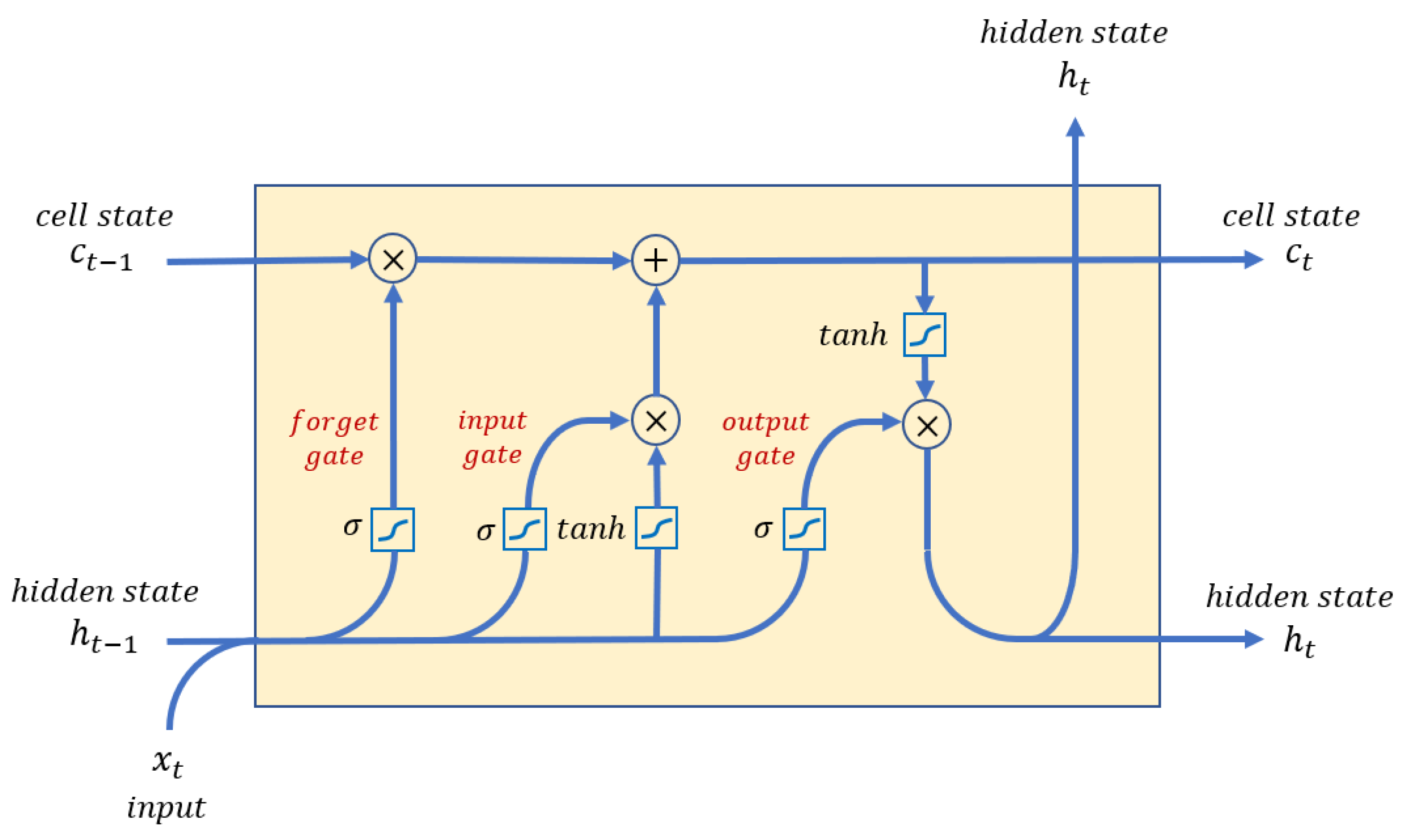
The TimeGAN hyperparameters determined in this section are the sequence length and number of hidden units of the LSTM networks. In these experiments, the hyperparameters for the evaluation networks of Table 6 were used instead of the values of the hyperparameters obtained in Appendix B.1.

Three experiments were performed with 16, 24, 32, 40, and 48 timesteps sequences to determine the most appropriate values for the TimeGAN sequence length hyperparameter. This length must be obtained carefully, as a very small value may not be sufficient to capture a practically useful sequence, while a very long sequence may require a large amount of resources and processing time. The results of the experiments to find the discriminative scores are shown in Table A4, where it can be observed that the best average result of 0.158865 is obtained when using a sequence of length 24.

Table A4. Discriminative scores by length of the sequences.

Experiment	Sequence Length
	16	24	32	40	48
1	0.178690	0.126977	0.424268	0.378498	0.338867
2	0.122583	0.172577	0.294302	0.394288	0.373359
3	0.470293	0.177041	0.162676	0.463736	0.300644
Average	0.257189	0.158865	0.293875	0.412174	0.337623

Table A4. Discriminative scores by length of the sequences.

Experiment	Sequence Length
	16	24	32	40	48
1	0.178690	0.126977	0.424268	0.378498	0.338867
2	0.122583	0.172577	0.294302	0.394288	0.373359
3	0.470293	0.177041	0.162676	0.463736	0.300644
Average	0.257189	0.158865	0.293875	0.412174	0.337623

The results of the experiments carried out with the predictive network are shown in Table A5, which shows that the best average result of 0.081198 is achieved with sequences of length 24.

Table A5. Predictive scores by length of the sequences.

Experiment	Sequence Length
	16	24	32	40	48
1	0.079849	0.090120	0.084412	0.096048	0.096296
2	0.076416	0.077339	0.087748	0.079849	0.155386
3	0.096282	0.076136	0.077865	0.147370	0.119579
Average	0.084182	0.081198	0.083342	0.107756	0.123754

Table A5. Predictive scores by length of the sequences.

Experiment	Sequence Length
	16	24	32	40	48
1	0.079849	0.090120	0.084412	0.096048	0.096296
2	0.076416	0.077339	0.087748	0.079849	0.155386
3	0.096282	0.076136	0.077865	0.147370	0.119579
Average	0.084182	0.081198	0.083342	0.107756	0.123754

Appendix B.3. Determination of the Number of Hidden Units Hyperparameter in TimeGAN

Using the results from Appendix B.1 and Appendix B.2, three experiments were performed considering 20, 40, 60, 80, and 100 hidden units in TimeGAN networks to determine which value was the most appropriate for this hyperparameter.

Table A6 shows the results of the experiments to obtain the discriminative scores. It can be seen in this table that the best average value of 0.194983 was obtained with 80 hidden units.

Table A6. Discriminative scores by number of hidden units.

Experiment	No. of Hidden Units
	20	40	60	80	100
1	0.277360	0.388457	0.287181	0.126977	0.096046
2	0.323597	0.359566	0.301403	0.258291	0.285395
3	0.331443	0.184311	0.169898	0.199681	0.349235
Average	0.310799	0.310778	0.252827	0.194983	0.243559

Table A6. Discriminative scores by number of hidden units.

Experiment	No. of Hidden Units
	20	40	60	80	100
1	0.277360	0.388457	0.287181	0.126977	0.096046
2	0.323597	0.359566	0.301403	0.258291	0.285395
3	0.331443	0.184311	0.169898	0.199681	0.349235
Average	0.310799	0.310778	0.252827	0.194983	0.243559

The results for the predictive scores are indicated in Table A7, where it can be observed that the best average value for the three experiments of 0.084204 was obtained with 80 hidden units.

Table A7. Predictive scores by number of hidden units.

Experiment	No. of Hidden Units
	20	40	60	80	100
1	0.077949	0.086518	0.168168	0.090120	0.073495
2	0.096677	0.241468	0.081442	0.089779	0.144930
3	0.083645	0.074895	0.077272	0.072714	0.191932
Average	0.086090	0.134294	0.108961	0.084204	0.136786

Table A7. Predictive scores by number of hidden units.

Experiment	No. of Hidden Units
	20	40	60	80	100
1	0.077949	0.086518	0.168168	0.090120	0.073495
2	0.096677	0.241468	0.081442	0.089779	0.144930
3	0.083645	0.074895	0.077272	0.072714	0.191932
Average	0.086090	0.134294	0.108961	0.084204	0.136786

Appendix B.4. Final Hyperparameters of the Networks

In this section, the following values are determined: (1) the number of iterations of TimeGAN and (2) the number of iterations and batch size of the predictive network. Table A8 summarizes the best values found in Appendix B.2 and Appendix B.3.

Table A8. Final candidate TimeGAN hyperparameters.

TimeGAN Hyperparameter	Value
Sequence length	24
No. of hidden units	80

Table A8. Final candidate TimeGAN hyperparameters.

TimeGAN Hyperparameter	Value
Sequence length	24
No. of hidden units	80

It can be observed from Table A8 that the best value for the number of hidden units for TimeGAN networks is equal to 80 and that the best value for the sequence length is 24. We ran a set of experiments to observe the values of the scores when using several different numbers of hidden units close to 80, specifically, with 70, 80, and 90 hidden units. For the discriminative and predictive networks, the hyperparameters in Table 6 were updated with the values obtained in Appendix B.1.

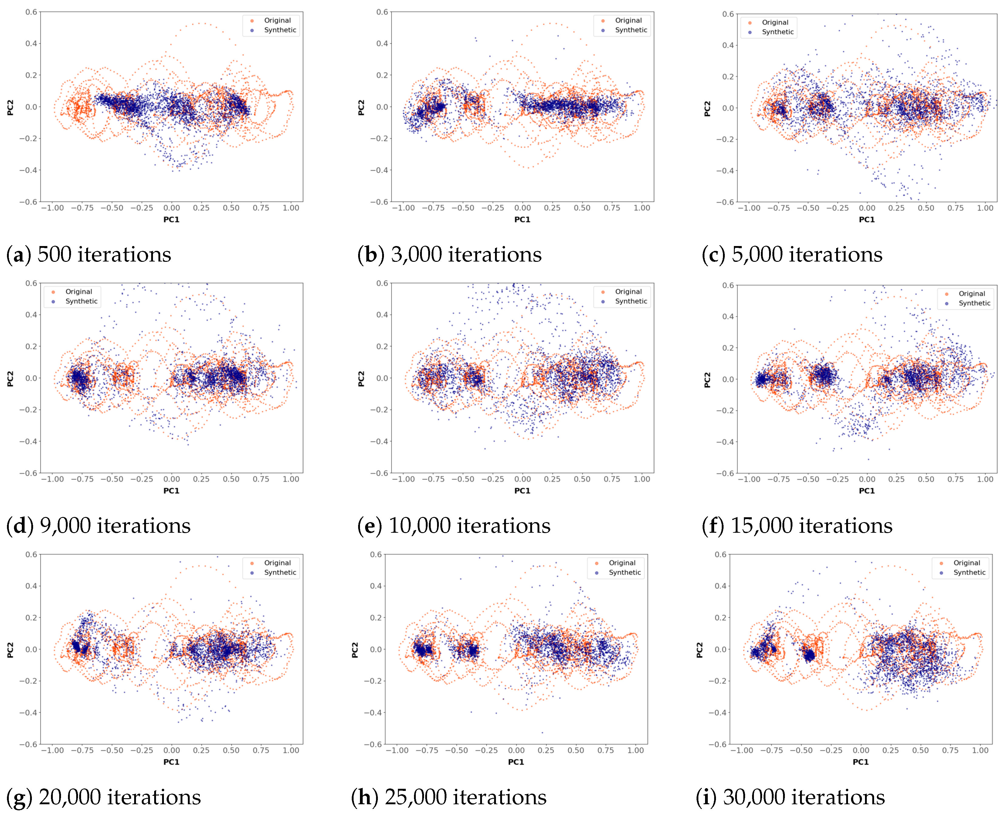
For our analysis of the discriminative scores, a series of 27 experiments were run, three for each number of hidden units for each of 500, 3000, 5000, 9000, 10,000, 15,000, 20,000, 25,000, and 30,000 iterations. This set of experiments allowed us to establish the best number of iterations to use when training the TimeGAN networks. After the first run of 27 experiments, the results shown in Table A9 were obtained.

Table A9. Discriminative scores for the first run of experiments.

No. of TimeGAN Iterations 1	Hidden Units	Discriminative Score
500	70	0.263010
	80	0.230102
	90	0.189796
3000	70	0.079337
	80	0.092730
	90	0.047959
5000	70	0.156378
	80	0.044643
	90	0.072126
9000	70	0.041199
	80	0.057908
	90	0.064413
10,000	70	0.045663
	80	0.050255
	90	0.055995
15,000	70	0.062883
	80	0.025510
	90	0.101913
20,000	70	0.075000
	80	0.075255
	90	0.054974
25,000	70	0.069005
	80	0.127296
	90	0.051148
30,000	70	0.076658
	80	0.068495
	90	0.134566

¹ The batch size and the number of iterations for the discriminative network were 32 and 200, respectively.

Table A9. Discriminative scores for the first run of experiments.

No. of TimeGAN Iterations 1	Hidden Units	Discriminative Score
500	70	0.263010
	80	0.230102
	90	0.189796
3000	70	0.079337
	80	0.092730
	90	0.047959
5000	70	0.156378
	80	0.044643
	90	0.072126
9000	70	0.041199
	80	0.057908
	90	0.064413
10,000	70	0.045663
	80	0.050255
	90	0.055995
15,000	70	0.062883
	80	0.025510
	90	0.101913
20,000	70	0.075000
	80	0.075255
	90	0.054974
25,000	70	0.069005
	80	0.127296
	90	0.051148
30,000	70	0.076658
	80	0.068495
	90	0.134566

¹ The batch size and the number of iterations for the discriminative network were 32 and 200, respectively.

Regarding the analysis of predictive scores, a series of fifteen experiments were run, three for each number of hidden units for each of 500, 3000, 5000, 9000, and 10,000 iterations. After the first run of fifteen experiments, the results shown in Table A10 were obtained.

Upon closely examining the predictive scores in Table A10, it can be noticed that the scores do not improve very much even when the number of TimeGAN iterations increases from 500 to 10,000, and seem to stagnate. For this reason, we used one of the following best values from the set of hyperparameters obtained in Appendix B.1 to perform a new set of experiments; in this case, the value of 8000 iterations was selected and used, instead of 500 for the discriminative network.

The variation of the predictive score on data generated with TimeGAN when changing the number of iterations of the predictive network was analyzed in experiments with 70, 80, and 90 hidden units and with 500, 2000, 5000, and 8000 iterations for the predictive network, all with 10,000 TimeGAN iterations. The results in Table A11 reflect a considerable improvement in the predictive scores with 70, 80, and 90 hidden units when increasing the number of iterations from 500 to 8000 in the predictive network. Therefore, this value was established as the new hyperparameter for the number of iterations of the predictive network.

Table A10. Predictive scores for the first run of experiments.

No. of TimeGAN Iterations 1	Hidden Units	Predictive Score
500	70	0.103060
	80	0.078703
	90	0.074426
3000	70	0.069205
	80	0.071240
	90	0.073169
5000	70	0.065946
	80	0.068529
	90	0.069467
9000	70	0.069823
	80	0.070330
	90	0.070437
10,000	70	0.070021
	80	0.068833
	90	0.065653

¹ The batch size and the number of iterations for the predictive network were 256 and 500, respectively.

Table A10. Predictive scores for the first run of experiments.

No. of TimeGAN Iterations 1	Hidden Units	Predictive Score
500	70	0.103060
	80	0.078703
	90	0.074426
3000	70	0.069205
	80	0.071240
	90	0.073169
5000	70	0.065946
	80	0.068529
	90	0.069467
9000	70	0.069823
	80	0.070330
	90	0.070437
10,000	70	0.070021
	80	0.068833
	90	0.065653

¹ The batch size and the number of iterations for the predictive network were 256 and 500, respectively.

Table A11. Predictive scores by number of iterations in the predictive network.

Number of	Number of Iterations in the Predictive Network 1
Hidden Units	500	2000	5000	8000
70	0.070021	0.054281	0.047422	0.044132
80	0.068833	0.052964	0.043623	0.039589
90	0.065653	0.053009	0.047998	0.043958
Average	0.068169	0.053418	0.046348	0.042560

¹ The batch size for the predictive network in these experiments was 256, while the number of iterations for TimeGAN networks was 10,000.

Table A11. Predictive scores by number of iterations in the predictive network.

Number of	Number of Iterations in the Predictive Network 1
Hidden Units	500	2000	5000	8000
70	0.070021	0.054281	0.047422	0.044132
80	0.068833	0.052964	0.043623	0.039589
90	0.065653	0.053009	0.047998	0.043958
Average	0.068169	0.053418	0.046348	0.042560

¹ The batch size for the predictive network in these experiments was 256, while the number of iterations for TimeGAN networks was 10,000.

The 27 experiments were then run again using the value of 8000 instead of 500 for the number of iterations of the predictive network and keeping its batch size fixed at 256. The results after applying this change are shown in Table A12.

Table A12. Predictive scores for first fit of predictive network values.

No. of TimeGAN Iterations 1	Hidden Units	Predictive Score
500	70	0.120283
	80	0.068555
	90	0.069589
3000	70	0.053960
	80	0.048301
	90	0.052339
5000	70	0.047269
	80	0.046167
	90	0.051160
9000	70	0.049712
	80	0.045722
	90	0.048057
10,000	70	0.044132
	80	0.039589
	90	0.043958
15,000	70	0.045661
	80	0.045869
	90	0.050569
20,000	70	0.045642
	80	0.051687
	90	0.046660
25,000	70	0.050789
	80	0.054795
	90	0.048775
30,000	70	0.044212
	80	0.048324
	90	0.055946

¹ In these experiments, the batch size and number of iterations in the predictive network were kept constant at 256 and 8000, respectively.

Table A12. Predictive scores for first fit of predictive network values.

No. of TimeGAN Iterations 1	Hidden Units	Predictive Score
500	70	0.120283
	80	0.068555
	90	0.069589
3000	70	0.053960
	80	0.048301
	90	0.052339
5000	70	0.047269
	80	0.046167
	90	0.051160
9000	70	0.049712
	80	0.045722
	90	0.048057
10,000	70	0.044132
	80	0.039589
	90	0.043958
15,000	70	0.045661
	80	0.045869
	90	0.050569
20,000	70	0.045642
	80	0.051687
	90	0.046660
25,000	70	0.050789
	80	0.054795
	90	0.048775
30,000	70	0.044212
	80	0.048324
	90	0.055946

¹ In these experiments, the batch size and number of iterations in the predictive network were kept constant at 256 and 8000, respectively.

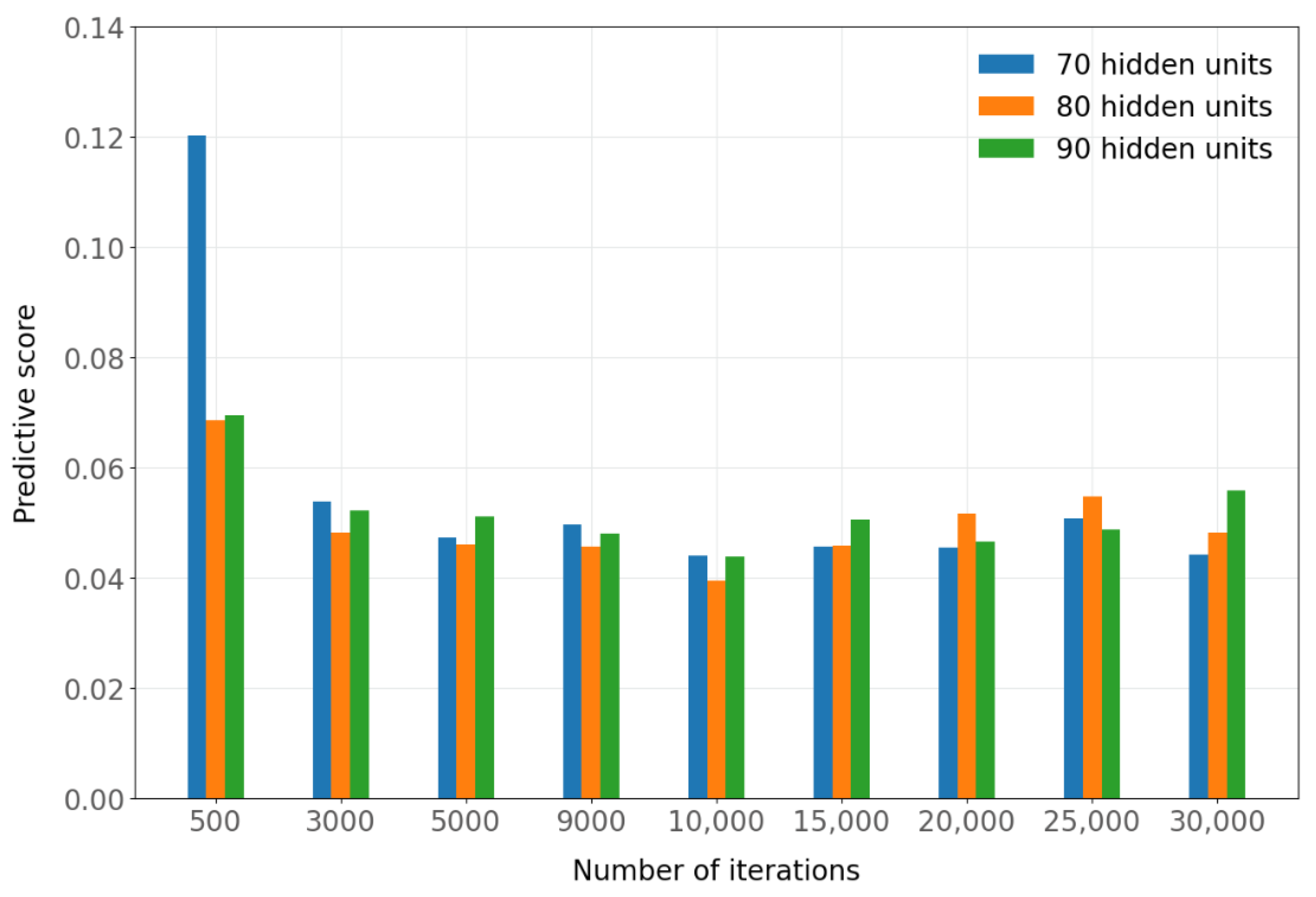
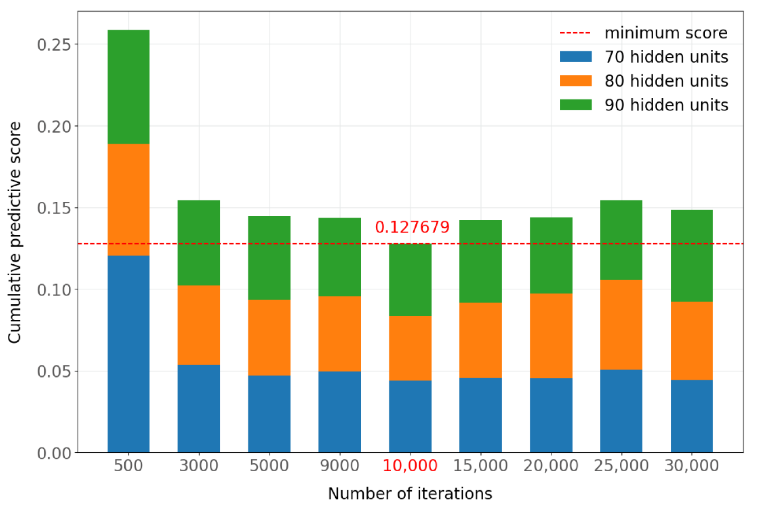
Figure A2 shows the predictive scores corresponding to Table A12. Figure A3 shows an alternative way of looking at the results of Figure A2, showing the cumulative predictive scores for 70, 80, and 90 hidden units for each number of iterations considered. This figure shows that the lowest (best) sum of the scores occurred when 10,000 iterations were used in TimeGAN. Similar results were obtained when the experiments were repeated with 8000 iterations and a batch size of 512 instead of 256 for the predictive network, with a slight improvement in training time. Table A13 compares the predictive scores when using batch sizes 256 and 512 in the predictive network. 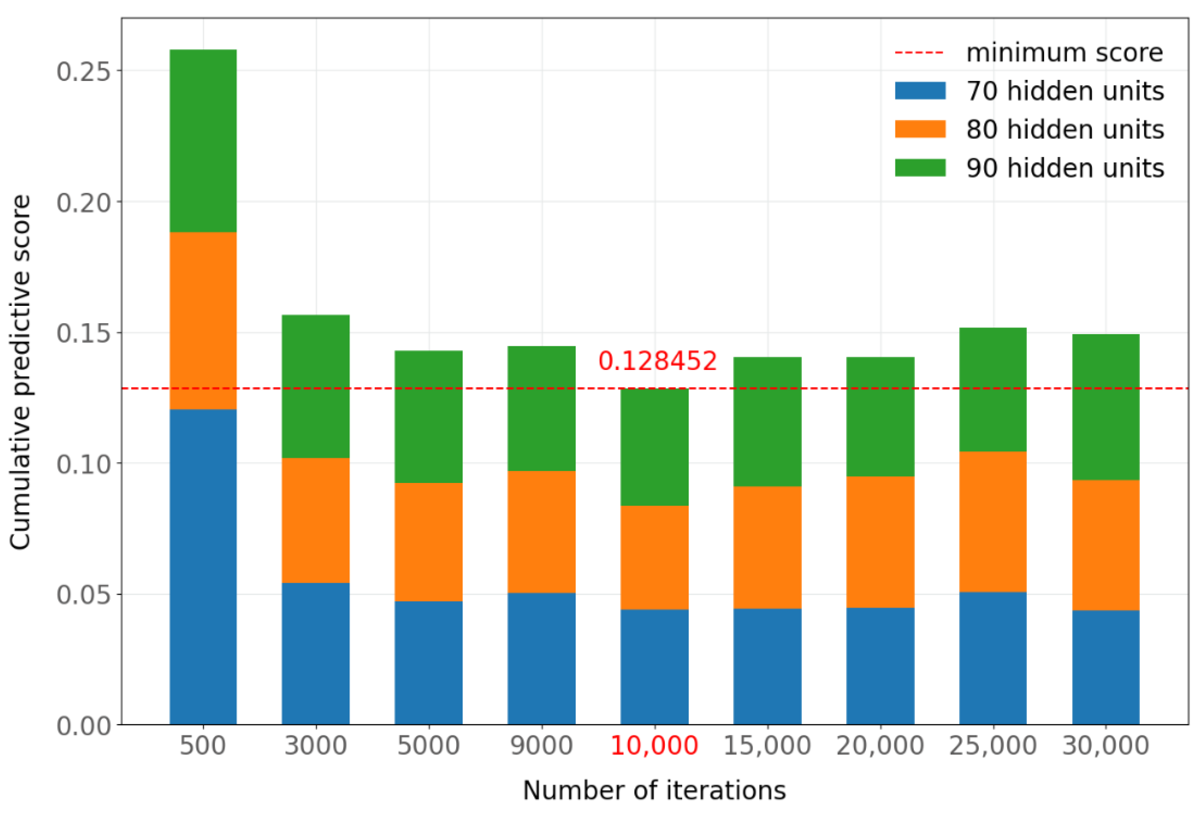Figure A4 shows the predictive scores with a batch size of 512. The cumulative scores for each number of iterations with a batch size of 512 are shown in Figure A5, where the best value is obtained with 10,000 iterations. When comparing the results obtained with batch sizes of 256 and 512 in the predictive network, quite similar values are obtained, with 0.127679 for a batch size of 256 and 0.128452 for a batch size of 512. In this case, 512 was chosen as the value of the batch size hyperparameter because it required a slightly shorter training time.

Table A13. Comparison between adjusted predictive scores for different batch sizes.

No. of TimeGAN Iterations 1	Hidden Units	Predictive Score (Batch Size = 256)	Predictive Score (Batch Size = 512)
500	70	0.120283	0.120361
	80	0.068555	0.067848
	90	0.069589	0.069784
3000	70	0.053960	0.054237
	80	0.048301	0.047550
	90	0.052339	0.054814
5000	70	0.047269	0.047083
	80	0.046167	0.045364
	90	0.051160	0.050311
9000	70	0.049712	0.050340
	80	0.045722	0.046526
	90	0.048057	0.047894
10,000	70	0.044132	0.044151
	80	0.039589	0.039535
	90	0.043958	0.044766
15,000	70	0.045661	0.044439
	80	0.045869	0.046439
	90	0.050569	0.049636
20,000	70	0.045642	0.044827
	80	0.051687	0.050140
	90	0.046660	0.045477
25,000	70	0.050789	0.050622
	80	0.054795	0.053755
	90	0.048775	0.047294
30,000	70	0.044212	0.043546
	80	0.048324	0.049939
	90	0.055946	0.055648

¹ In these experiments, the sequence length was kept constant at 24.

Table A13. Comparison between adjusted predictive scores for different batch sizes.

No. of TimeGAN Iterations 1	Hidden Units	Predictive Score (Batch Size = 256)	Predictive Score (Batch Size = 512)
500	70	0.120283	0.120361
	80	0.068555	0.067848
	90	0.069589	0.069784
3000	70	0.053960	0.054237
	80	0.048301	0.047550
	90	0.052339	0.054814
5000	70	0.047269	0.047083
	80	0.046167	0.045364
	90	0.051160	0.050311
9000	70	0.049712	0.050340
	80	0.045722	0.046526
	90	0.048057	0.047894
10,000	70	0.044132	0.044151
	80	0.039589	0.039535
	90	0.043958	0.044766
15,000	70	0.045661	0.044439
	80	0.045869	0.046439
	90	0.050569	0.049636
20,000	70	0.045642	0.044827
	80	0.051687	0.050140
	90	0.046660	0.045477
25,000	70	0.050789	0.050622
	80	0.054795	0.053755
	90	0.048775	0.047294
30,000	70	0.044212	0.043546
	80	0.048324	0.049939
	90	0.055946	0.055648

¹ In these experiments, the sequence length was kept constant at 24.

Figure A2. Predictive score by number of iterations of the predictive network (batch size = 256).

Figure A3. Cumulative score by number of iterations of the predictive network (batch size = 256).

Figure A4. Predictive score by number of iterations of the predictive network (batch size = 512).

Figure A5. Cumulative score by number of iterations of the predictive network (batch size = 512).

Appendix B.5. Final Hyperparameters

In Appendix B.1, Appendix B.2, Appendix B.3 and Appendix B.4, the best values for the hyperparameters of TimeGAN and the evaluation networks were found. The experiments that produced the best results for the evaluation networks are shown in Table A14.

Table A14. Best candidate scores for the evaluation networks.

No. of TimeGAN Iterations	Hidden Units	Discriminative Score	Predictive Score
15,000	80	0.025510	0.046439
10,000	80	0.050255	0.039535

Table A14. Best candidate scores for the evaluation networks.

No. of TimeGAN Iterations	Hidden Units	Discriminative Score	Predictive Score
15,000	80	0.025510	0.046439
10,000	80	0.050255	0.039535

The best discriminative and predictive scores were obtained with different numbers of iterations in TimeGAN; the best discriminative score was 0.025510, obtained with 15,000 iterations, while the best predictive score was 0.039535, obtained with 10,000 iterations. It was necessary to choose one of these two numbers of iterations as the final TimeGAN hyperparameter. The value of 10,000 was preferred as the hyperparameter value for the following reasons: (1) it required less training time, and (2) the cumulative discriminative scores with 10,000 iterations were lower than those obtained with 15,000 iterations.

In Appendix B.3, we identified that the best value for the number of hidden units hyperparameter of TimeGAN was 80; however, the closest values to 80 that were considered in that analysis were 60 and 100. The results in this appendix establish that the best number of iterations to generate data with TimeGAN is 10,000; furthermore, the results in Table A9 indicate that the best discriminative score for that number of iterations is 0.045663, which is obtained with 70 hidden units. For this reason, we updated the hidden units hyperparameter from 80 to 70. Table A15 shows the final hyperparameters that produced the best experimental results.

Table A15. Final TimeGAN hyperparameters.

No. of TimeGAN Iterations	Sequence Length	Hidden Units
10,000	24	70

Table A15. Final TimeGAN hyperparameters.

No. of TimeGAN Iterations	Sequence Length	Hidden Units
10,000	24	70

References

- Esteban, C.; Hyland, S.L.; Rätsch, G. Real-valued (Medical) Time Series Generation with Recurrent Conditional GANs. arXiv 2017, arXiv:1706.02633. [Google Scholar]
- Lin, Z.; Jain, A.; Wang, C.; Fanti, G.; Sekar, V. Using GANs for Sharing Networked Time Series Data: Challenges, Initial Promise, and Open Questions. In Proceedings of the ACM Internet Measurement Conference, New York, NY, USA, 27–29 October 2020; IMC ’20. pp. 464–483. [Google Scholar] [CrossRef]
- Lu, P.H.; Wang, P.C.; Yu, C.M. Empirical Evaluation on Synthetic Data Generation with Generative Adversarial Network. In Proceedings of the 9th International Conference on Web Intelligence, Mining and Semantics, New York, NY, USA, 26–28 June 2019; WIMS2019. pp. 1–6. [Google Scholar] [CrossRef]
- Leznik, M.; Michalsky, P.; Willis, P.; Schanzel, B.; Östberg, P.O.; Domaschka, J. Multivariate Time Series Synthesis Using Generative Adversarial Networks. In Proceedings of the ACM/SPEC International Conference on Performance Engineering, New York, NY, USA, 19–23 April 2021; ICPE ’21. pp. 43–50. [Google Scholar] [CrossRef]
- Patterson, J.; Gibson, A. Deep Learning: A Practitioner’s Approach; O’Reilly: Sebastopol, CA, USA, 2017. [Google Scholar]
- Goodfellow, I.; Pouget-Abadie, J.; Mirza, M.; Xu, B.; Warde-Farley, D.; Ozair, S.; Courville, A.; Bengio, Y. Generative Adversarial Networks. Commun. ACM 2020, 63, 139–144. [Google Scholar] [CrossRef]
- Jaafer, A.; Nilsson, G.; Como, G. Data Augmentation of IMU Signals and Evaluation via a Semi-Supervised Classification of Driving Behavior. In Proceedings of the 2020 IEEE 23rd International Conference on Intelligent Transportation Systems (ITSC), Rhodes, Greece, 20–23 September 2020; pp. 1–6. [Google Scholar] [CrossRef]
- Lakshminarayanan, M.; Channegowda, J.; Herle, A.; Prabhu, D.; Chaudhari, S. Generating high-fidelity synthetic battery parameter data: Solving sparse dataset challenges. Int. J. Energy Res. 2021, 45, 16856–16864. [Google Scholar] [CrossRef]
- Li, J.; Liu, Y.; Li, Q. Generative Adversarial Network and Transfer Learning Based Fault Detection for Rotating Machinery with Imbalance Data Condition. Meas. Sci. Technol. 2021, 33, 045103. [Google Scholar] [CrossRef]
- Luo, Y.; Cai, X.; Zhang, Y.; Xu, J.; Yuan, X. Multivariate Time Series Imputation with Generative Adversarial Networks. In Proceedings of the 32nd International Conference on Neural Information Processing Systems, Red Hook, NY, USA, 3–8 December 2018; NIPS’18. pp. 1603–1614. [Google Scholar]
- Yoon, J.; Jarrett, D.; van der Schaar, M. Time-series Generative Adversarial Networks. In Proceedings of the Advances in Neural Information Processing Systems; Wallach, H., Larochelle, H., Beygelzimer, A., d’Alché-Buc, F., Fox, E., Garnett, R., Eds.; Curran Associates, Inc.: Red Hook, NY, USA, 2019; Volume 32, pp. 1–11. [Google Scholar]
- Brownlee, J. Basics of Linear Algebra for Machine Learning: Discover the Mathematical Language of Data in Python; Machine Learning Mastery: San Juan, Puerto Rico, 2018. [Google Scholar]
- Jansen, S. Hands-On Machine Learning for Algorithmic Trading: Design and Implement Investment Strategies Based on Smart Algorithms That Learn from Data Using Python; Packt Publishing: Birmingham, UK, 2018. [Google Scholar]
- Pei, H.; Ren, K.; Yang, Y.; Liu, C.; Qin, T.; Li, D. Towards Generating Real-World Time Series Data. In Proceedings of the 2021 IEEE International Conference on Data Mining (ICDM), Los Alamitos, CA, USA, 7–10 December 2021; pp. 469–478. [Google Scholar] [CrossRef]
- Asre, S.; Anwar, A. Synthetic Energy Data Generation Using Time Variant Generative Adversarial Network. Electronics 2022, 11, 355. [Google Scholar] [CrossRef]
- Liu, L.M.; Ren, X.Y.; Zhang, F.; Gao, L.; Hao, B. Dual-dimension Time-GGAN data augmentation method for improving the performance of deep learning models for PV power forecasting. Energy Rep. 2023, 9, 6419–6433. [Google Scholar] [CrossRef]
- Sabry, F.; Labda, W.; Ahmed Eltaras, T.; Hamza, F.; Elzoubi, K.; Malluhi, Q. Wearable Data Generation Using Time-Series Generative Adversarial Networks for Hydration Monitoring. In Proceedings of the 16th International Joint Conference on Biomedical Engineering Systems and Technologies, BIOSTEC 2023, Volume 4: BIOSIGNALS, Lisbon, Portugal, 16–18 February 2023; pp. 94–105. [Google Scholar] [CrossRef]
- Yang, L.; Yuan, J.; Zhao, X.; Fang, S.; He, Z.; Zhan, J.; Hu, Z.; Li, X. SceGAN: A Method for Generating Autonomous Vehicle Cut-In Scenarios on Highways Based on Deep Learning. J. Intell. Connect. Veh. 2023, 6, 264–274. [Google Scholar] [CrossRef]
- Alzantot, M.; Chakraborty, S.; Srivastava, M.B. SenseGen: A Deep Learning Architecture for Synthetic Sensor Data Generation. arXiv 2017, arXiv:1701.08886. [Google Scholar] [CrossRef]
- Delaney, A.M.; Brophy, E.; Ward, T.E. Synthesis of Realistic ECG using Generative Adversarial Networks. arXiv 2019, arXiv:1909.09150. [Google Scholar] [CrossRef]
- Demetriou, A.; Alfsvåg, H.; Rahrovani, S.; Haghir Chehreghani, M. A Deep Learning Framework for Generation and Analysis of Driving Scenario Trajectories. SN Comput. Sci. 2023, 4, 251. [Google Scholar] [CrossRef]
- Ganti, B.; Chaitanya, G.; Balamurugan, R.S.; Nagaraj, N.; Balasubramanian, K.; Pati, S. Time-Series Generative Adversarial Network Approach of Deep Learning Improves Seizure Detection From the Human Thalamic SEEG. Front. Neurol. 2022, 13, 755094. [Google Scholar] [CrossRef] [PubMed]
- Haradal, S.; Hayashi, H.; Uchida, S. Biosignal Data Augmentation Based on Generative Adversarial Networks. In Proceedings of the 2018 40th Annual International Conference of the IEEE Engineering in Medicine and Biology Society (EMBC), Honolulu, HI, USA, 18–21 July 2018; pp. 368–371. [Google Scholar] [CrossRef]
- Hazra, D.; Byun, Y.C. SynSigGAN: Generative Adversarial Networks for Synthetic Biomedical Signal Generation. Biology 2020, 9, 441. [Google Scholar] [CrossRef] [PubMed]
- Hui, S.; Wang, H.; Wang, Z.; Yang, X.; Liu, Z.; Jin, D.; Li, Y. Knowledge Enhanced GAN for IoT Traffic Generation. In Proceedings of the ACM Web Conference 2022, New York, NY, USA, 25–29 April 2022; WWW ’22. pp. 3336–3346. [Google Scholar] [CrossRef]
- Purwita, A.A.; Yesilkaya, A.; Haas, H. Synthetic LiFi Channel Model Using Generative Adversarial Networks. In Proceedings of the ICC 2022-IEEE International Conference on Communications, Seoul, Republic of Korea, 16–20 May 2022; pp. 577–582. [Google Scholar] [CrossRef]
- Haleem, M.S.; Ekuban, A.; Antonini, A.; Pagliara, S.; Pecchia, L.; Allocca, C. Deep-Learning-Driven Techniques for Real-Time Multimodal Health and Physical Data Synthesis. Electronics 2023, 12, 1989. [Google Scholar] [CrossRef]
- Anande, T.; Alsaadi, S.; Leeson, M. Generative adversarial networks for network traffic feature generation. Int. J. Comput. Appl. 2023, 45, 297–305. [Google Scholar] [CrossRef]
- Hartmann, K.G.; Schirrmeister, R.T.; Ball, T. EEG-GAN: Generative adversarial networks for electroencephalograhic (EEG) brain signals. arXiv 2018, arXiv:1806.01875. [Google Scholar] [CrossRef]
- Yılmaz, B. Generative adversarial network for load data generation: Türkiye energy market case. Math. Model. Numer. Simul. Appl. 2023, 3, 141–158. [Google Scholar] [CrossRef]
- Aznan, N.; Atapour Abarghouei, A.; Bonner, S.; Connolly, J.; Al Moubayed, N.; Breckon, T. Simulating Brain Signals: Creating Synthetic EEG Data via Neural-Based Generative Models for Improved SSVEP Classification. In Proceedings of the 2019 International Joint Conference on Neural Networks (IJCNN), Budapest, Hungary, 14–19 July 2019; pp. 1–8. [Google Scholar] [CrossRef]
- Ramponi, G.; Protopapas, P.; Brambilla, M.; Janssen, R. T-CGAN: Conditional Generative Adversarial Network for Data Augmentation in Noisy Time Series with Irregular Sampling. arXiv 2019, arXiv:cs.LG/1811.08295. [Google Scholar]
- Zhang, C.; Kuppannagari, S.R.; Kannan, R.; Prasanna, V.K. Generative Adversarial Network for Synthetic Time Series Data Generation in Smart Grids. In Proceedings of the 2018 IEEE International Conference on Communications, Control, and Computing Technologies for Smart Grids (SmartGridComm), Aalborg, Denmark, 29–31 October 2018; pp. 1–6. [Google Scholar] [CrossRef]
- Li, X.; Metsis, V.; Wang, H.; Ngu, A.H.H. TTS-GAN: A Transformer-based Time-Series Generative Adversarial Network. In Proceedings of the Conference on Artificial Intelligence in Medicine in Europe, Halifax, NS, Canada, 14–17 June 2022; pp. 133–143. [Google Scholar]
- Naveed, M.H.; Hashmi, U.S.; Tajved, N.; Sultan, N.; Imran, A. Assessing Deep Generative Models on Time Series Network Data. IEEE Access 2022, 10, 64601–64617. [Google Scholar] [CrossRef]
- Wang, W.; Xi, J.; Chong, A.; Li, L. Driving Style Classification Using a Semisupervised Support Vector Machine. IEEE Trans. Hum.-Mach. Syst. 2017, 47, 650–660. [Google Scholar] [CrossRef]
- Khodairy, M.; Abo Samra, G.A.A. Driving Behavior Classification Based on Oversampled Signals of Smartphone Embedded Sensors Using an Optimized Stacked-LSTM Neural Networks. IEEE Access 2021, 9, 4957–4972. [Google Scholar] [CrossRef]
- Wang, S.; Ma, C.; Xu, Y.; Wang, J.; Wu, W. A Hyperparameter Optimization Algorithm for the LSTM Temperature Prediction Model in Data Center. Sci. Program. 2022, 2022, 1–13. [Google Scholar] [CrossRef]
- Marcillo, P.; Barona López, L.I.; Valdivieso Caraguay, Á.L.; Hernández-Álvarez, M. Modeling of a Vehicle Accident Prediction System Based on a Correlation of Heterogeneous Sources. In Advances in Intelligent Systems and Computing; Springer: Cham, Switzerland, 2020; Volume 1212 AISC, pp. 260–266. [Google Scholar] [CrossRef]
Disclaimer/Publisher’s Note: The statements, opinions and data contained in all publications are solely those of the individual author(s) and contributor(s) and not of MDPI and/or the editor(s). MDPI and/or the editor(s) disclaim responsibility for any injury to people or property resulting from any ideas, methods, instructions or products referred to in the content. |
© 2024 by the authors. Licensee MDPI, Basel, Switzerland. This article is an open access article distributed under the terms and conditions of the Creative Commons Attribution (CC BY) license (https://creativecommons.org/licenses/by/4.0/).