Cooling Load Forecasting Method for Central Air Conditioning Systems in Manufacturing Plants Based on iTransformer-BiLSTM

Abstract

Cooling load forecasting is a crucial aspect of optimizing energy efficiency and efficient operation in central air conditioning systems for manufacturing plants. Due to the influence of multiple factors, the cooling load in manufacturing plants exhibits complex characteristics, including multi-peak patterns, periodic fluctuations, and short-term disturbances during meal periods. Existing methods struggle to accurately capture the relationships among variables and temporal dependencies, leading to limited forecasting accuracy. To address these challenges, this paper proposes a hybrid forecasting method based on the iTransformer-BiLSTM. First, the Pearson correlation coefficient is employed to select time-series variables that have a significant impact on cooling load. Then, iTransformer is utilized for feature extraction to capture nonlinear dependencies among multivariate inputs and global temporal patterns. Finally, BiLSTM is applied for temporal modeling, leveraging its bidirectional recurrent structure to capture both forward and backward dependencies in time series, thereby improving forecasting accuracy. Experimental validation on a cooling load dataset from a welding workshop in a manufacturing plant, including ablation studies and comparative analyses with other algorithms, demonstrates that the proposed method achieves superior performance compared to traditional approaches in forecasting accuracy. Meanwhile, by integrating the SHAP sensitivity analysis method, the contributions of input variables to the cooling load prediction results are systematically evaluated, thereby enhancing the interpretability of the model. This research provides a reliable technical foundation for energy-efficient control of central air conditioning systems in manufacturing plants.

1. Introduction

As the scale of the manufacturing industry expands and energy consumption demands rise, air conditioning system energy consumption accounts for 30–50% of the total energy consumption in factory buildings [1,2], making it a significant source of carbon emissions in factories. However, traditional building automation systems rely on real-time feedback regulation and lack the foresight to predict cooling load trends. This results in delayed responses during significant fluctuations in cooling load [3], leading to energy waste, reduced operational efficiency, and difficulties in maintaining indoor thermal comfort. Accurate cooling load prediction can optimize air conditioning system parameters (e.g., chiller start/stop times, pump frequency adjustments) in advance, dynamically matching actual demand and reducing redundant cooling. Meanwhile, the multi-peak characteristic, periodic fluctuations, and timely disturbances (e.g., during meal times) of factory cooling load require the model to capture the multivariable coupling relationships and complex time-series features that affect the load. Therefore, precise cooling load prediction is a key technology for energy-saving and consumption reduction in factories. It not only reduces building energy costs and extends equipment lifespan but also improves thermal comfort in workshops, ensures production processes, and supports the manufacturing industry’s transition to low-carbon and intelligent operations, making it of significant practical importance for achieving dual-carbon goals.

Cooling load prediction is an important part of designing and operating building air conditioning systems. There are currently two main approaches: mechanism-based modeling and data-driven modeling [4,5], each suitable for different application fields. Mechanism-based modeling relies on the physical characteristics of buildings and thermodynamic principles to describe the internal thermal equilibrium processes through mathematical equations. It requires detailed information such as building structure, internal heat source distribution, usage characteristics, and external environmental conditions to establish a building thermodynamic model. Tools such as EnergyPlus [6], TRNSYS [7], and DeST [8] are often used to simulate building cooling load. However, due to difficulties in obtaining building parameters, high computational complexity, and limited flexibility, mechanism-based modeling is typically used during the air conditioning design phase and is less suitable for dynamic cooling load prediction during the operational phase.

Data-driven modeling uses historical data from air conditioning systems to establish load prediction models through machine learning and deep learning techniques. This approach offers advantages such as data intuitiveness, high flexibility, fast modeling, and strong learning capabilities, making it widely used in energy-efficient operation optimization of air conditioning systems in recent years.

Numerous scholars both domestically and internationally have conducted extensive research on data-driven modeling for air conditioning cooling load prediction, evolving from single-method data-driven modeling to combined modeling methods. The single data-driven modeling approach has evolved from early classical statistical methods to machine learning techniques, such as Support Vector Regression [9,10,11,12], and BP Neural Networks [13,14,15]. In recent years, deep learning methods have also become a prominent research focus in the field of air conditioning cooling load prediction.

With the increasing accuracy requirements for load prediction, multivariable data fusion, hybrid model optimization, and improvements in hyperparameter optimization algorithms have become key development directions for air conditioning cooling load prediction models. He Ning et al. [16] proposed an LBF cooling load combined prediction model based on LSTM, BP, and particle filters, which integrates the advantages of multiple algorithms and achieves superior prediction accuracy and robustness in air conditioning load forecasting applications. Sajjad M et al. [17] proposed a hybrid sequence learning prediction model that combines CNN and GRU. By utilizing CNN to extract key features from the data and inputting them into a multi-layer GRU for sequence learning, this method outperforms the single GRU model in terms of accuracy and generalization ability. References [18,19,20] also employ CNN to extract features from the input data, reducing input dimensions while improving prediction accuracy. Although CNN can effectively extract local features, its ability to capture global information is limited [21], which may affect prediction accuracy in nonlinear and dynamic load forecasting tasks. Moreover, traditional sequence models (such as LSTM and GRU) can alleviate the vanishing gradient problem [22], but still face issues such as high computational cost, limited capacity to capture long-range dependencies, insufficient global feature modeling, and poor scalability when handling long sequences.

The Transformer model has demonstrated significant advantages in global information modeling and long-range dependency capture due to its powerful self-attention mechanism [23]. However, it still has limitations in local feature extraction and model stability. Traditional Transformer prediction models typically integrate the time-step variable features (Tokens) in a time series into a single high-dimensional vector (Temporal Token), encode the time-step features through a feed-forward network (FFN), and capture the relationships between time steps using attention mechanisms [24]. However, this method has significant flaws: variables with different physical meanings are forced into the same Token, which can introduce noise due to distribution differences or time lags, making it difficult to accurately represent the interactions between variables. Moreover, processing Tokens in time-step order leads to high computational complexity and inefficiency [25], and the limited local receptive field prevents the model from effectively capturing long-sequence dependencies.

In recent years, although some studies have combined Transformer and RNN models or applied them individually in fields such as water level prediction [26,27,28], power output forecasting [29,30], and trajectory prediction [31,32], their applications in HVAC systems, particularly in cooling load prediction tasks for manufacturing factories, remain limited. Compared to the datasets in the aforementioned fields, cooling load data from factory workshops exhibit pronounced nonlinearity, multi-peak periodic fluctuations, and strong multivariate coupling characteristics. These include the intertwined effects of outdoor meteorological conditions, indoor environmental parameters, and variations in production processes, which collectively lead to highly complex and challenging time-series modeling. Existing models based solely on Transformer or RNN architectures face limitations in this context, often demonstrating insufficient local feature extraction or inadequate global dependency capture when modeling such multi-source heterogeneous time-series data, thereby restricting further improvements in prediction accuracy.

Therefore, this paper proposes an iTransformer-BiLSTM hybrid prediction method for cooling load, using iTransformer to capture the global nonlinear relationships between multiple variables and BiLSTM to extract the time-series local features of the variables. This method achieves global-local feature collaborative modeling, significantly improving cooling load prediction accuracy under complex conditions and providing effective technical support for air conditioning energy optimization in manufacturing factories.

2. Materials and Methods

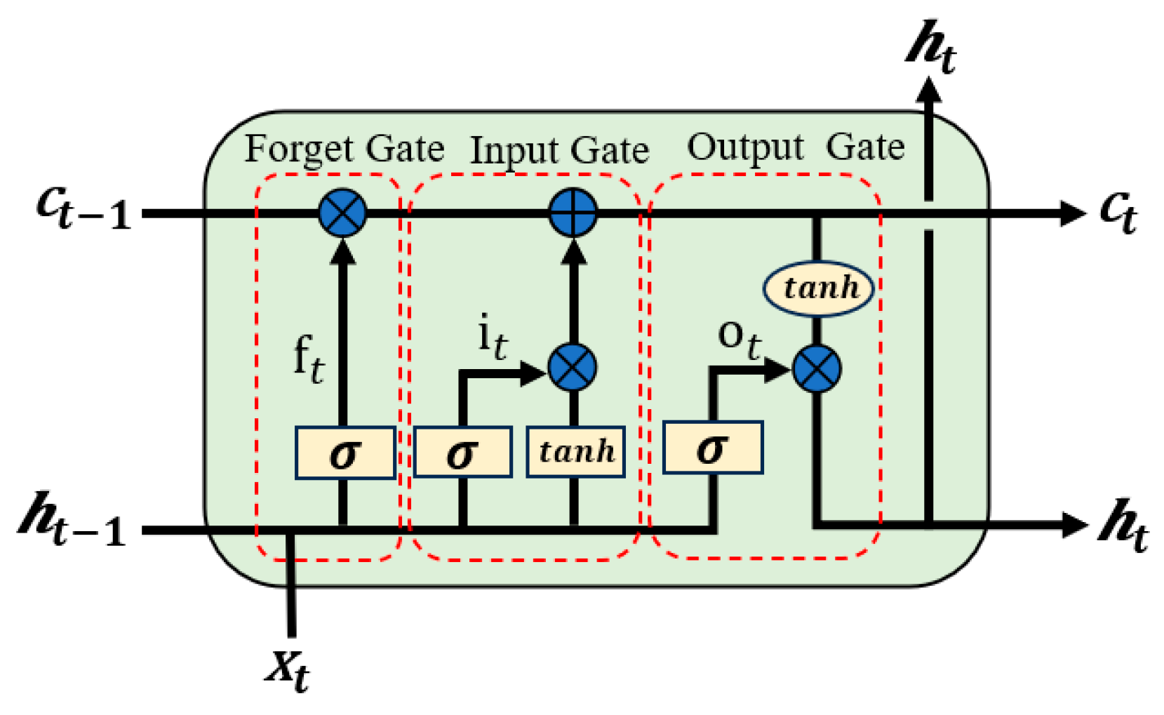
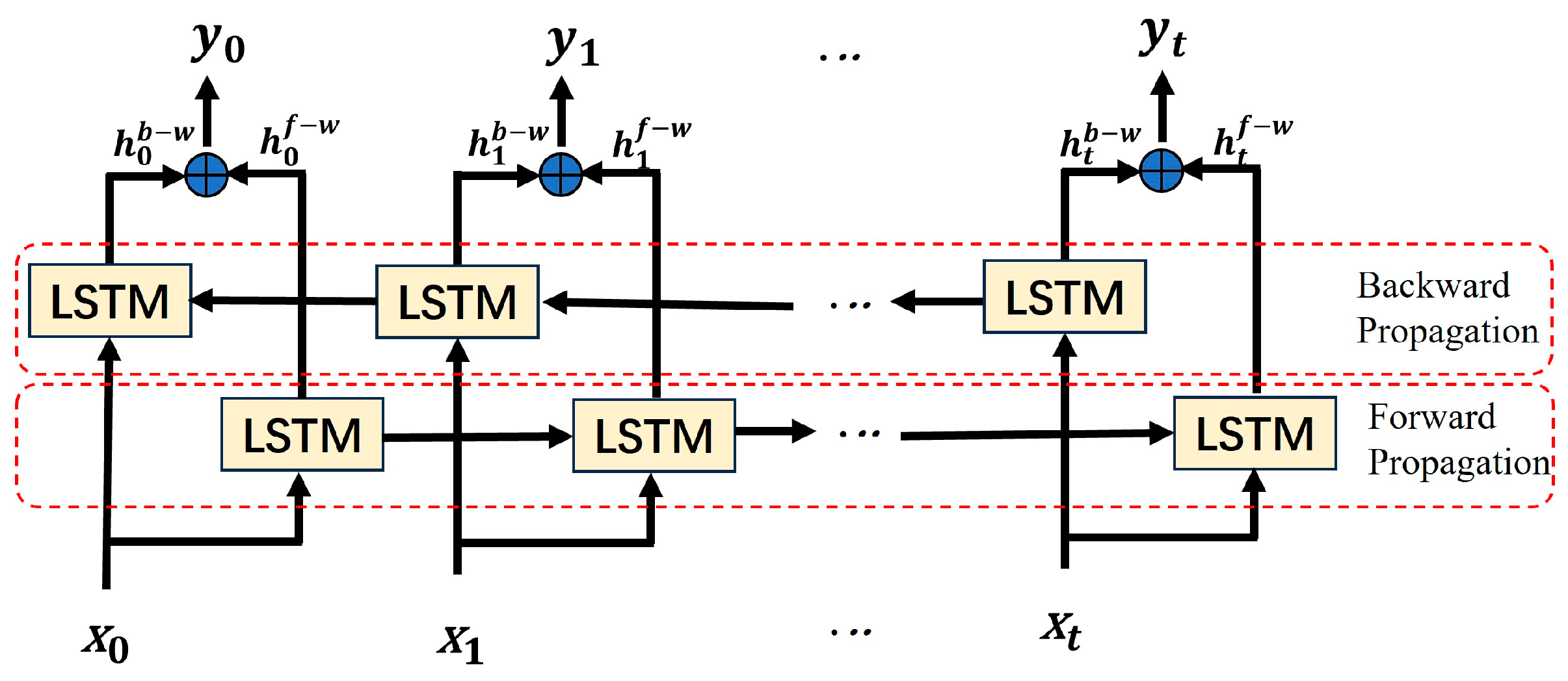
2.1. Bidirectional Long Short-Term Memory Network (BiLSTM) Model

BiLSTM is a deep learning model based on Recurrent Neural Networks (RNNs) that is widely applied in temporal data modeling. The architecture of LSTM was specifically designed to address the vanishing gradient and exploding gradient problems that commonly affect traditional RNNs when processing long-term dependencies [33]. By incorporating gating mechanisms (input gate, forget gate, and output gate), LSTM dynamically regulates information flow pathways, enabling the network to selectively retain or discard temporal information, thereby enhancing its capacity for modeling long-term sequence features. The structure of LSTM is illustrated in Figure 1, with its computational process represented by the following equations:

$$\left\{\begin{array}{l}{f}_t=\sigma (W_f\left[h_{t-1},x_t\right]+b_f)\\ i_t=\sigma (W_i\left[h_{t-1},x_t\right]+b_i)\\ {\tilde{C}}_t=\tanh (W_c\left[h_{t-1},x_t\right]+b_c)\\ C_t=f_t\ast C_{t-1}+i_t\ast {\tilde{C}}_t\\ o_t=\sigma (W_o\left[h_{t-1},x_t\right]+b_o)\\ h_t=o_t\ast \tanh (C_t)\end{array}\right.$$

(1)

where $f_t$ represents the forget gate, $i_t$ represents the input gate, $o_t$ represents the output gate, $C_t$ and $h$ represent the cell memory and the hidden state, respectively, $W$ and $b$ represent the weights and biases of the network, and $\sigma$ and $\tanh$ represent the activation functions.

Although LSTM mitigates the vanishing gradient problem through its gating mechanism, it may still face the challenge of information attenuation when processing ultra-long time series data. Additionally, traditional LSTM relies solely on unidirectional temporal information flow, meaning that predictions at the current time step are based only on past information and cannot fully utilize future time steps’ data. This limitation may reduce its ability to capture temporal features effectively. BiLSTM further extends the modeling capability of LSTM by introducing a bidirectional information propagation mechanism (forward and backward), allowing it to learn temporal dependencies from both past and future time steps, thus capturing contextual information in time series data more comprehensively. The core idea is to use a forward LSTM to process the time series from the start to the end, while a backward LSTM processes the time series from the end to the start. The forward and backward hidden states are then fused to enhance the model’s ability to capture global temporal features. In the cooling load forecasting task in manufacturing plants, the load data often exhibit complex characteristics such as multi-peak and periodic fluctuations. BiLSTM, by merging forward and backward information, improves the model’s ability to represent these features, enabling it to adapt well to load changes at different time scales. The BiLSTM structure is shown in Figure 2. In this figure, BiLSTM takes multivariate time series data with a history step size of t and N variables as input, learns the forward hidden state ${\overrightarrow{\mathrm{h}}}_{\mathrm{t}}$ and the backward hidden state ${\overleftarrow{\mathrm{h}}}_{\mathrm{t}}$ through the forward and backward LSTMs, and then concatenates and fuses them into $H_t$. The final output $y_t$ is obtained through the output layer. The corresponding formulas are as follows:

$$\left\{\begin{array}{l}{\overrightarrow{h}}_t=LST{M}_{forward}(x_t,{\overrightarrow{h}}_{t-1})\\ {\overleftarrow{h}}_t=LST{M}_{backward}(x_t,{\overleftarrow{h}}_{t-1})\\ H_t=[{\overrightarrow{h}}_t,{\overleftarrow{h}}_t]\\ y_t=Outputlayer(H_t)\end{array}\right.$$

(2)

BiLSTM is essentially still a type of recurrent network, which processes multivariate time series data on a time-step basis. Each time step contains multiple feature values, and through bidirectional information interaction (forward and backward), it can effectively capture the temporal dependencies in multivariate time series. However, it has certain limitations when handling complex, long multivariate time series information. First, when facing long time series data, as the number of time steps increases, issues such as information loss or high model complexity leading to inefficient computation may arise. Secondly, BiLSTM lacks a specific mechanism to capture the complex nonlinear relationships in multivariate sequences, and there is a deficiency in capturing long-term interaction information between variables [34], especially in high-dimensional datasets. On the other hand, the iTransformer model, built upon the traditional Transformer, inverts the roles of the attention mechanism and the feed-forward neural network. It treats the entire time series of multivariate input variables as a token and uses its multi-head attention mechanism to effectively learn the complex nonlinear relationships between multivariate time series, compensating for the shortcomings of BiLSTM in processing complex multivariate time series information.

2.2. iTransformer Model

iTransformer is an improved Transformer model proposed by Yong Liu et al. in 2023 [35], which has achieved significant breakthroughs in complex multivariate time series forecasting tasks. iTransformer consists only of the encoder part and is composed of three main components: an embedding layer, multiple stackable Transformer modules, and a projection layer, as shown in Figure 3.

Given a multivariate time series dataset $X=\left\{{\mathrm{x}}_1,{\mathrm{x}}_2,\cdots ,{\mathrm{x}}_{\mathrm{T}}\right\}\in R^{T\times N}$ with a historical time step length of $T$ and $N$ variables, iTransformer first maps each variable’s sequence into a D-dimensional feature space through the embedding layer, obtaining a high-dimensional feature representation $h_n^0$. Each variable’s feature vector is referred to as a “Variate Token”, which contains all temporal variation information of that variable over the past $T$ time steps, encoding the entire sequence into a single token. The feature vectors of all variables form a matrix $H\in \left\{h_1,h_2,\cdots ,h_N\right\}\in R^{N\times D}$, which represents the sequential characteristics of each variable in the multivariate time series.

Compared to the Transformer model, iTransformer has an advantage in the embedding strategy, as it treats the entire time series segment as an independent variable (as shown in Figure 4), preserving the independence of each variable and avoiding the information mixing phenomenon during the embedding process in the traditional Transformer model. Meanwhile, iTransformer also reverses the roles of the multi-head self-attention mechanism and the position-wise feed-forward neural network in the Transformer: the traditional Transformer’s multi-head self-attention mechanism mainly models the temporal dependencies of the same variable at different historical time steps, but its ability to model cross-variable interaction dependencies is limited; in contrast, iTransformer’s multi-head attention mechanism is used to capture dependencies among different variables, while its position-wise feed-forward neural network is responsible for extracting the temporal characteristics of each variable, thus achieving the modeling and learning of the spatiotemporal dependencies of input variables. Within each Variate Token, layer normalization is applied to unify the measurement units and feature distributions among variables, accelerating model convergence and improving model stability. Moreover, since the decoder of the Transformer adopts an autoregressive prediction approach, which is prone to error accumulation, iTransformer directly projects each Variate Token through a projection layer implemented by a multi-layer perceptron (MLP), adopting a multi-task learning-like approach to directly output the final prediction result ${\widehat{Y}}_{:,n}$ of each variable, rather than using a decoder to generate predictions. The entire process can be expressed as the following computational workflow:

$$h_n^0=Embedding(X:,n)$$

(3)

$$H^{l+1}=TrmBlock(H^i),l=0,1,\cdots ,L-1$$

(4)

$${\widehat{Y}}_{:,n}=\mathrm{Pr}ojection({h_n}^l)$$

(5)

where $X:,n$ represents the entire sequence of the $n$th variable, ${\widehat{Y}}_{:,n}$ denotes the feature representation at the $i$th layer, and ${\widehat{Y}}_{:,n}$ represents the model’s predicted data for the $n$th variable.

In the TrmBlock component, the multi-head attention mechanism computes attention weights for the multivariate time series variables after positional encoding. By assigning high weights to key features, it captures the nonlinear relationships between variables. The calculation formula is as follows:

$$\left\{\begin{array}{l}Q=W^{Q}X\\ K=W^{K}X\\ V=W^{V}X\end{array}\right.$$

(6)

$$Attentio{n}_i=\mathrm{softmax}({\displaystyle \frac{Q{K}^T}{\sqrt{d_k}}})V$$

(7)

$$MultiHead(Q,K,V)=Concat(Attentio{n}_1,Attentio{n}_2,\cdot \cdot \cdot ,Attentio{n}_i)W^O$$

(8)

where $X$ represents the input multivariate time series matrix; $Q$, $K$, and $V$ are the query, key, and value matrices, respectively. $W^Q$, $W^K$, and $W^V$ are the learned weight matrices; $d_k$ is the scaling factor; $\mathrm{Softmax}$ is the activation function; $Concat$ is the concatenation function; $W^O$ is a learnable weight matrix responsible for the linear transformation of the concatenated outputs from multiple attention heads; $Attentio{n}_i$ represents the attention distribution of the $i$th head, and $MultiHead(Q,K,V)$ denotes the multi-head attention distribution.

When iTransformer is directly used for prediction, its projection layer maps the multivariate feature information extracted by the TrmBlock module directly to the final predicted values of the target variables. However, in this study, the iTransformer is utilized for feature extraction, where its output forms a high-dimensional feature matrix for each variable, denoted as $X\in R^{N\times d}$ (where N is the number of variables and d is the feature dimension). In this context, the projection layer is used to structurally reorganize the principal multivariate features extracted by the TrmBlock module, transforming them into a time-dominant input format compatible with subsequent models (such as BiLSTM). The specific process is as follows:

$$x_t=MLP([X;p_t]),t=1,2,\cdots ,T$$

(9)

where $p_t$ denotes the learnable positional encoding at time step t, and MLP represents the multi-layer perceptron. By inputting the feature variables and positional encodings output by the iTransformer, a feature representation $x_t\in R^d$ is generated for each time step. These representations are ultimately combined to form a sequential feature matrix $X^{\prime }\in R^{T\times d}$, which serves as the input to the BiLSTM. This process achieves the mapping from variable space to temporal sequence space, enabling the model to effectively capture the dynamic dependencies of cooling load variations over time.

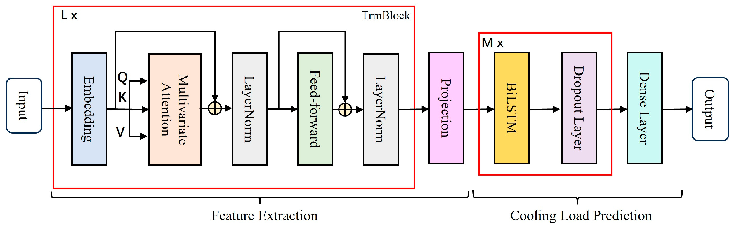
2.3. iTransformer-BiLSTM Prediction Method

This study proposes a hybrid iTransformer-BiLSTM prediction method, as shown in Figure 5. The method leverages the advantages of both global feature extraction and local temporal modeling to achieve high-precision cooling load prediction in complex industrial scenarios. The method takes multivariate time series data (including outdoor temperature, humidity, indoor temperature, historical load, and other features) as input. First, the iTransformer module, through multi-head attention and feedforward neural networks, encodes the entire time series of each variable as independent tokens, avoiding the noise interference from cross-variable embeddings in traditional Transformers, and fully exploring the nonlinear interactions and global dependencies between variables. Considering that the output of the iTransformer is organized along the variable axis, this study introduces a projection layer with positional awareness to transform it into a time-axis feature sequence, thereby achieving the structural alignment required by the BiLSTM. On this basis, the BiLSTM module captures the forward and backward dependencies of local temporal features through a bidirectional gated recurrent mechanism, and combines with a dropout layer to mitigate overfitting risks. Finally, the cooling load prediction value is output through a fully connected layer. Compared to single models, this hybrid approach integrates the global modeling capability of iTransformer for cross-variable interactions and the temporal dynamic analysis advantage of BiLSTM, significantly improving the prediction performance for multi-peak and periodic cooling load fluctuations.

3. Case Analysis

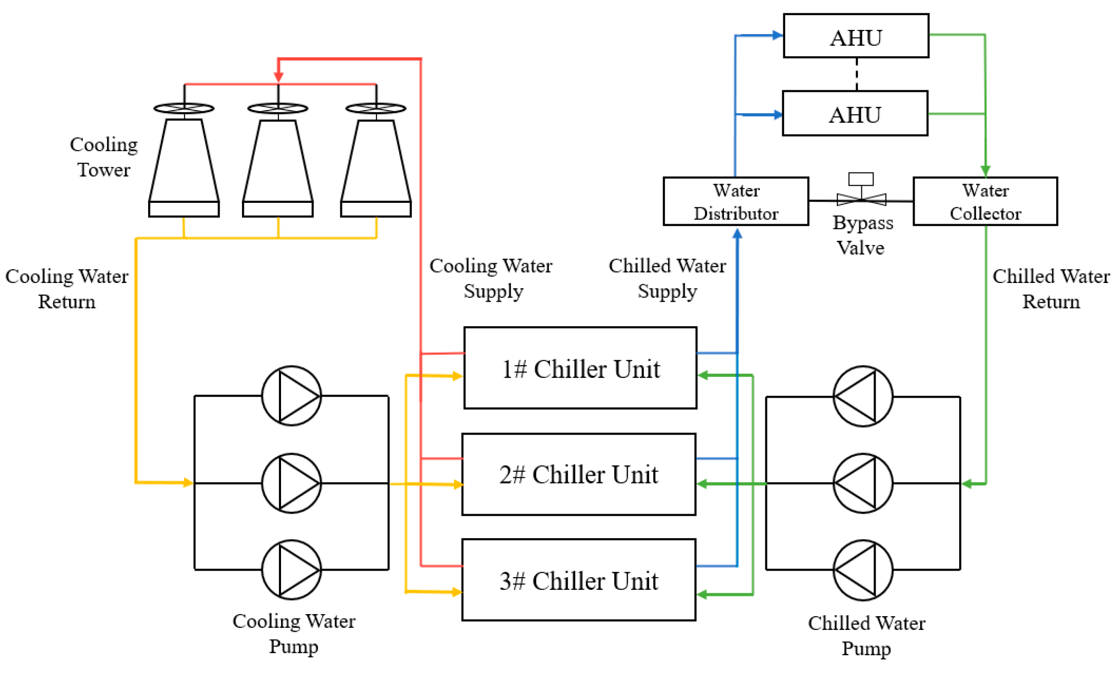
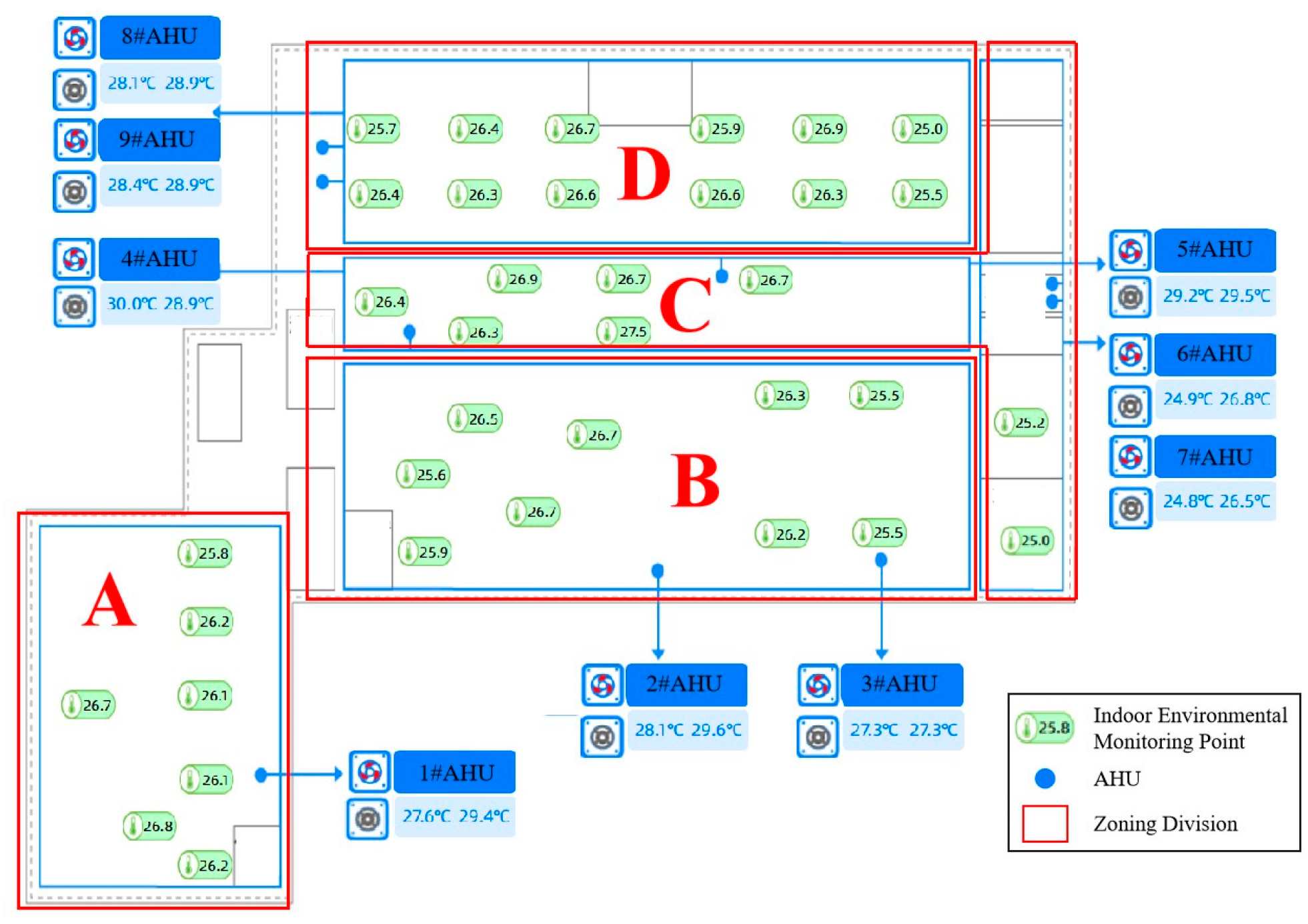
3.1. Research Object

This study focuses on the cooling load of the central air conditioning system in the welding workshop of an automobile manufacturing factory located in South China. The workshop covers an area of approximately 15,000 m², with a single-story structure, although some areas (such as the office) have a two-story design. The workshop primarily handles laser automated welding of automobile chassis and the assembly and quality inspection of components such as side panels and car doors. The air conditioning system’s cooling capacity is mainly designed to meet worker comfort requirements, operating during work hours and shutting down after hours, exhibiting certain periodicity. The cooling source system is equipped with two 2110 kW and one 2400 kW water-cooled chillers, with three chilled water pumps, cooling pumps, and cooling towers. The system structure of the cooling source is shown in Figure 6. The terminal system is equipped with nine air handling units. The author’s team was commissioned to carry out energy-saving modifications to the system and build an energy-saving control platform, which collects multi-dimensional data at a frequency of 15 min, including outdoor temperature, humidity, wet bulb temperature, indoor air handling unit supply and return air temperature, and environmental point temperature. The temperature point distribution and division in the factory workshop are shown in Figure 7. The internal temperature points, which take into account the layout of the internal space and the distribution of air handling unit ducts, are divided into four areas: A, B, C, and D.

3.2. Data Preprocessing

Due to factors such as sensor anomalies, network failures, and other noise interferences, the data collected and stored by the platform contains missing values and outliers. In this study, the quartile method is used to identify and remove outliers. The remaining data, along with the originally missing data, are then completed using cubic spline interpolation. Furthermore, to eliminate the impact of differences in the magnitudes of different variables on model accuracy, the data are normalized using the min-max normalization method, which is formulated as follows:

$$x^{\prime }(i)={\displaystyle \frac{x(i)-x_{\min }}{x_{\max }-x_{\min }}}$$

(10)

where $x(i)$ and $x^{\prime }(i)$ represent the values before and after normalization, respectively, and $x_{\max }$ and $x_{\min }$ are the maximum and minimum values of the variable sequence, respectively.

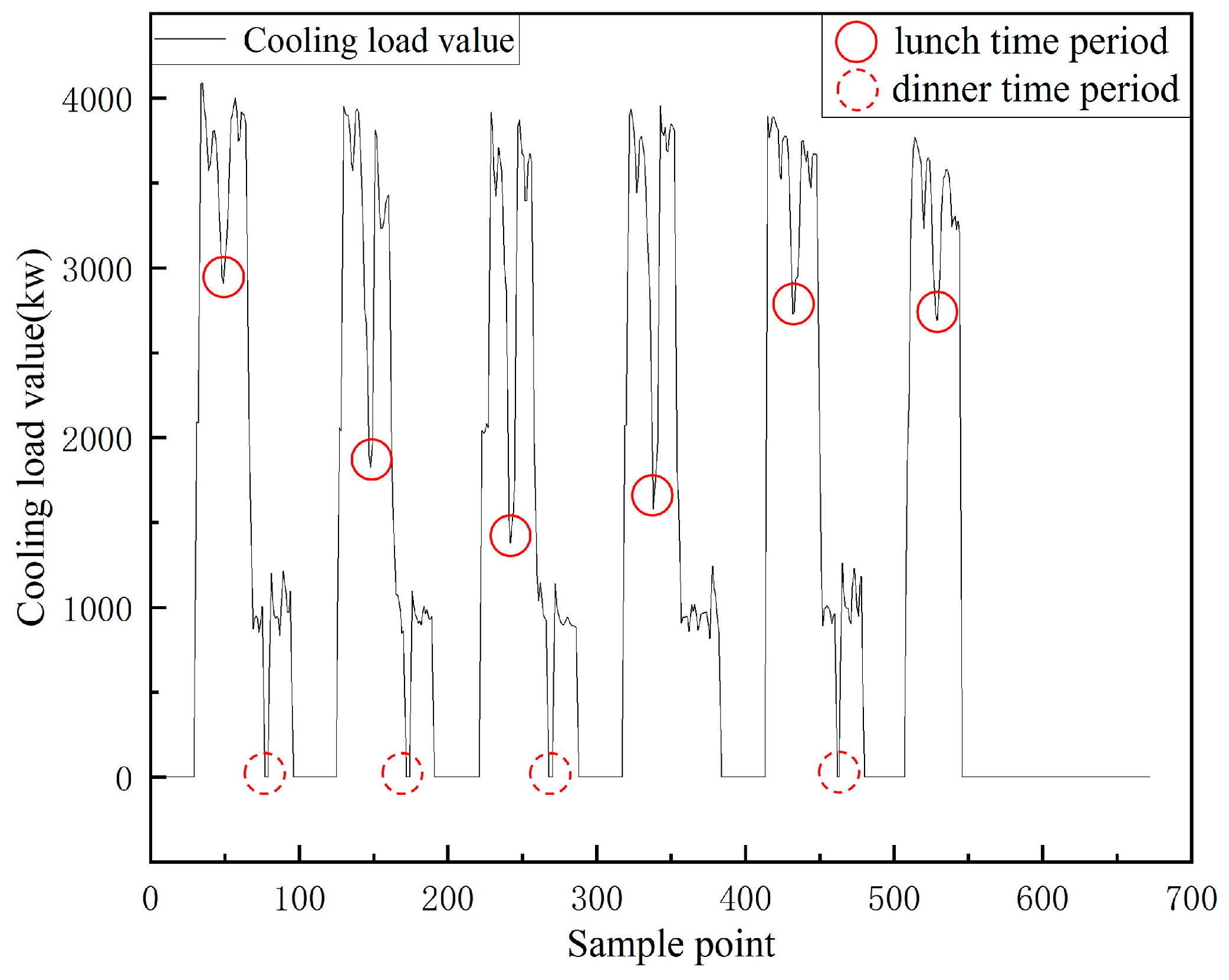
3.3. Analysis of Cooling Load Characteristics and Influencing Factors

The cooling load monitoring data for the workshop in June 2024 and the first week of June are shown in Figure 8 and Figure 9. The data indicate that the cooling load exhibits multi-peak characteristics and periodic fluctuations, with strong nonlinearity and instability. As observed in Figure 8, the cooling load is higher during daytime working hours when workers are densely engaged in operations. During lunch and dinner breaks, the cooling load demand decreases temporarily as workers leave the workshop for meals, followed by a subsequent increase. After dinner, the cooling load demand drops to approximately 50% of the daytime peak due to a reduction in the number of workers, decreased production activities, and lower nighttime temperatures. These fluctuations are driven by multiple coupled factors:

Impact of human behavior: Workers’ schedules directly influence the intensity of air conditioning usage; Equipment operation and production tasks: The intermittent operation of production equipment, lighting, and other internal heat sources exacerbates sudden load fluctuations; Disturbance from outdoor meteorological parameters: Variations in outdoor temperature and humidity interact with the heat transfer processes of the workshop’s envelope, causing disturbances to the cooling load. These factors collectively result in strong nonlinearity and complex temporal characteristics of the cooling load, making it difficult for traditional prediction methods to model the multivariable coupling relationships, leading to significant accuracy degradation in scenarios with sudden short-term fluctuations (such as during meal breaks) and long-period variations (such as night shift loads). Therefore, a nonlinear modeling approach that integrates global dependencies and local temporal patterns is required to meet the high-precision demands for optimizing workshop operations.

This study categorizes the factors influencing the workshop’s cooling load into three main categories: building structure, internal heat sources, and outdoor meteorological parameters, as shown in

Table 1. Influencing Factors of the Cooling Load in the Workshop.

Influencing Factor	Specific Content
Building structure	The physical structure of the building, such as the material properties of the enclosure and the insulation performance of wall materials, etc.
Internal heat source	The internal heat sources of the workshop (such as the operation of production equipment, lighting systems, etc.), the number of employees, and their activity intensity.
Outdoor meteorological parameters	Environmental factors such as outdoor temperature, humidity, ground air pressure, wind speed, and solar radiation intensity.

. For workshops already in operation, the impact of static parameters such as building structure, materials, and orientation on the factory’s cooling load remains relatively stable, and thus can be simplified as constant values in the modeling process. Among outdoor meteorological parameters, solar radiation and wind speed exhibit high fluctuations and entail high monitoring costs. Therefore, in accordance with the following references [12,36], this study includes only outdoor temperature and humidity as input variables. The dynamic factors inside the workshop (such as equipment operation, lighting systems, and personnel activity) are indirectly represented as follows: equipment operation status, personnel count, and activity intensity are embedded in the historical cooling load time-series data, while the average temperature points of the four zones and the supply and return air temperatures of air handling units reflect the real-time heat source distribution. Additionally, dimensionality reduction is applied to mitigate the risk of overfitting caused by high-dimensional inputs. A Pearson correlation analysis is conducted among these terminal parameters, outdoor meteorological parameters, date attributes, and cooling load data, as shown in

Table 2. Influence of Various Factors on the Cooling Load.

Feature Name	Correlation Coefficient	Feature Name	Correlation Coefficient
Day of the Week	0.110	Average Supply Air Temperature in Zone C	−0.846
Temperature Differential Between Supply and Return Air of AHU in Zone D	0.880	Average Supply Air Temperature in Zone B	−0.789
Temperature Differential Between Supply and Return Air of AHU in Zone C	0.921	Average Supply Air Temperature in Zone A	−0.788
Temperature Differential Between Supply and Return Air of AHU in Zone B	0.894	Average Temperature in Zone D	−0.307
Temperature Differential Between Supply and Return Air of AHU in Zone A	0.886	Average Temperature in Zone C	−0.574
Average Return Air Temperature of AHU in Zone D	−0.141	Average Temperature in Zone B	−0.361
Average Return Air Temperature of AHU in Zone C	−0.044	Average Temperature in Zone A	−0.379
Average Return Air Temperature of AHU in Zone B	0.203	Outdoor Temperature	0.463
Average Return Air Temperature of AHU in Zone A	0.149	Wet Bulb Temperature	0.114
Average Supply Air Temperature in Zone D	−0.797	Outdoor Humidity	−0.336

.

As shown in Table 2, date attributes (such as the day of the week) have a weak impact on the cooling load and are therefore not considered as input features. Among the outdoor meteorological parameters of the factory workshop, outdoor temperature and humidity exhibit a high correlation with the cooling load, making them suitable as model input features. Regarding indoor parameters, the supply and return air temperature difference of the air handling units in the four zones shows the highest correlation with the supply air temperature, approximately 0.8. Considering that the supply and return air temperature difference is derived from the difference between the supply air temperature and the return air temperature, it serves as a more representative feature. Therefore, by comprehensively considering the influence of indoor and outdoor parameters, the final input features include the historical data of outdoor temperature, humidity, the supply and return air temperature difference of air handling units in the four zones, and the cooling load, totaling seven features, to predict future cooling load.

3.4. Evaluation and Analysis of Model Prediction Results

The cooling season from June to August 2024 (92 days, 8832 valid data points) is selected as the training set, while the period from September 1 to September 20 (20 days, 1920 data points) is used as the test set. Based on the factory’s early/late shift system (each shift lasting 8 h), an 8-h historical window (32 time steps) is set to predict the cooling load at the next time step. This window fully captures the load fluctuation cycle of a single shift, balancing temporal feature extraction and computational efficiency. The experiments are conducted on a Windows 11 operating system using MATLAB v2023b, with model construction performed via the Deep Learning Toolbox. Hyperparameters are determined through empirical tuning, with key configurations listed in

Table 3. Main Parameter Settings of the iTransformer-BiLSTM Model.

Model		Parameter Settings
iTransformer-BiLSTM	iTransformer	Number of encoder layers: 2, number of multi-head attention heads: 4, number of channels: 128.
	BiLSTM	Number of BiLSTM layers: 2, number of hidden units per layer: 64/32, Dropout rate: 0.05.
	other	Epoch: 256, learning rate: 0.002, optimizer: Adam, loss function: RMSE.

.

3.4.1. Model Evaluation Metrics

To evaluate the performance of the model, this study selects Root Mean Square Error (RMSE), Mean Absolute Error (MAE), and Symmetric Mean Absolute Percentage Error (SMAPE) as evaluation metrics. Their calculation formulas are as follows:

$$\mathrm{RMSE}=\sqrt{{\displaystyle \frac{1}{n}}{\displaystyle \sum _{i=1}^n{(y_i-{\widehat{y}}_i)}^2}}$$

(11)

$$\mathrm{MAE}={\displaystyle \frac{1}{n}}{\displaystyle \sum _{i=1}^n\left|y_i-{\widehat{y}}_i\right|}$$

(12)

$$\mathrm{SMAPE}={\displaystyle \frac{1}{n}}{\displaystyle \sum _{i=1}^n\frac{y-{\widehat{y}}_i}{(\left|y\right|+\left|{\widehat{y}}_i\right|)/2}}\times 100\%$$

(13)

In the formula, $y_i$ and ${\widehat{y}}_i$ represent the true value and the predicted value of the i-th sample, respectively; the value range of RMSE and MAE is [0, +∞]. The closer the value is to 0, the smaller the prediction error of the model is, and the better the performance is. The value range of SMAPE is [0, 200%], and the closer it is to 0, the better the model prediction effect is.

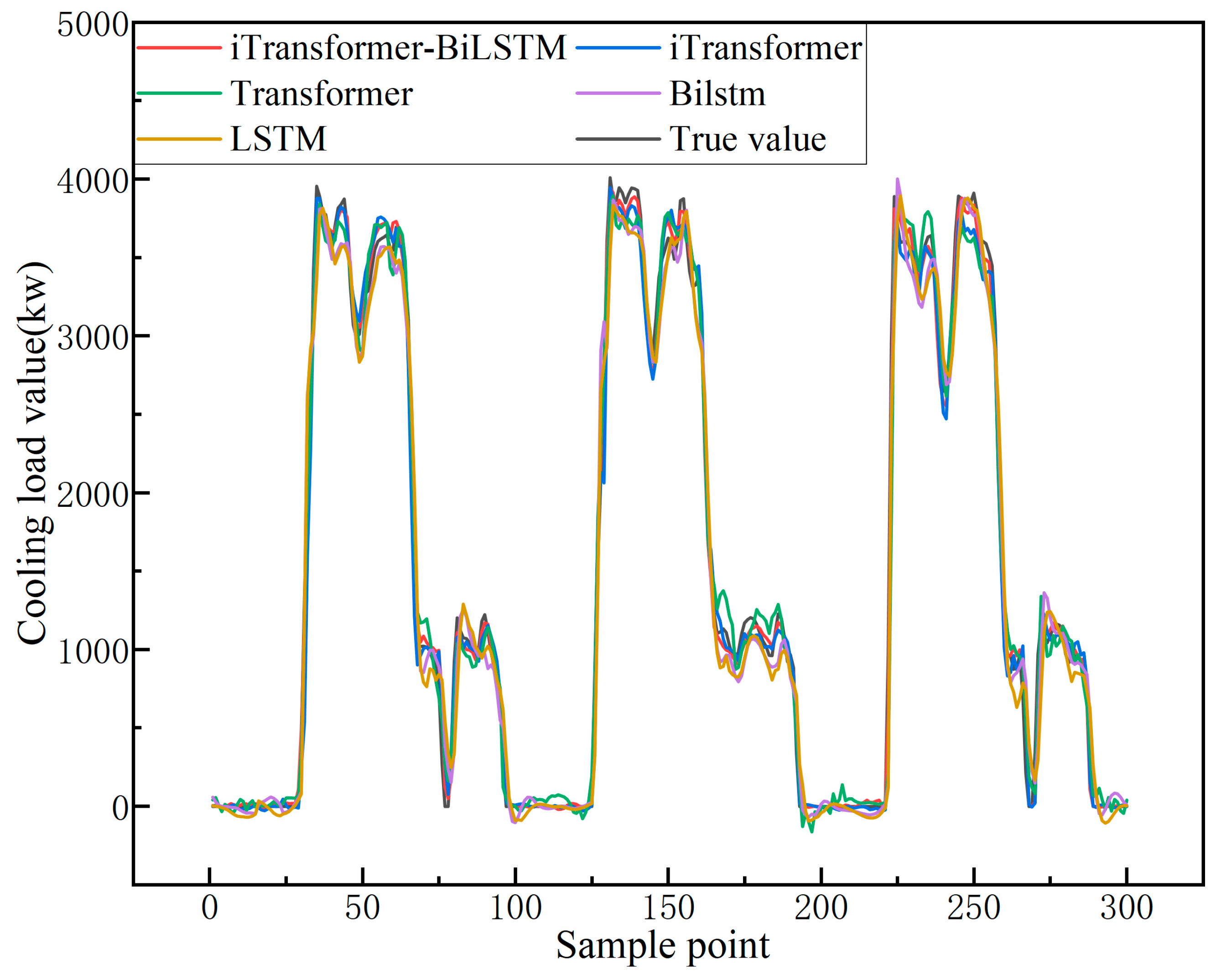
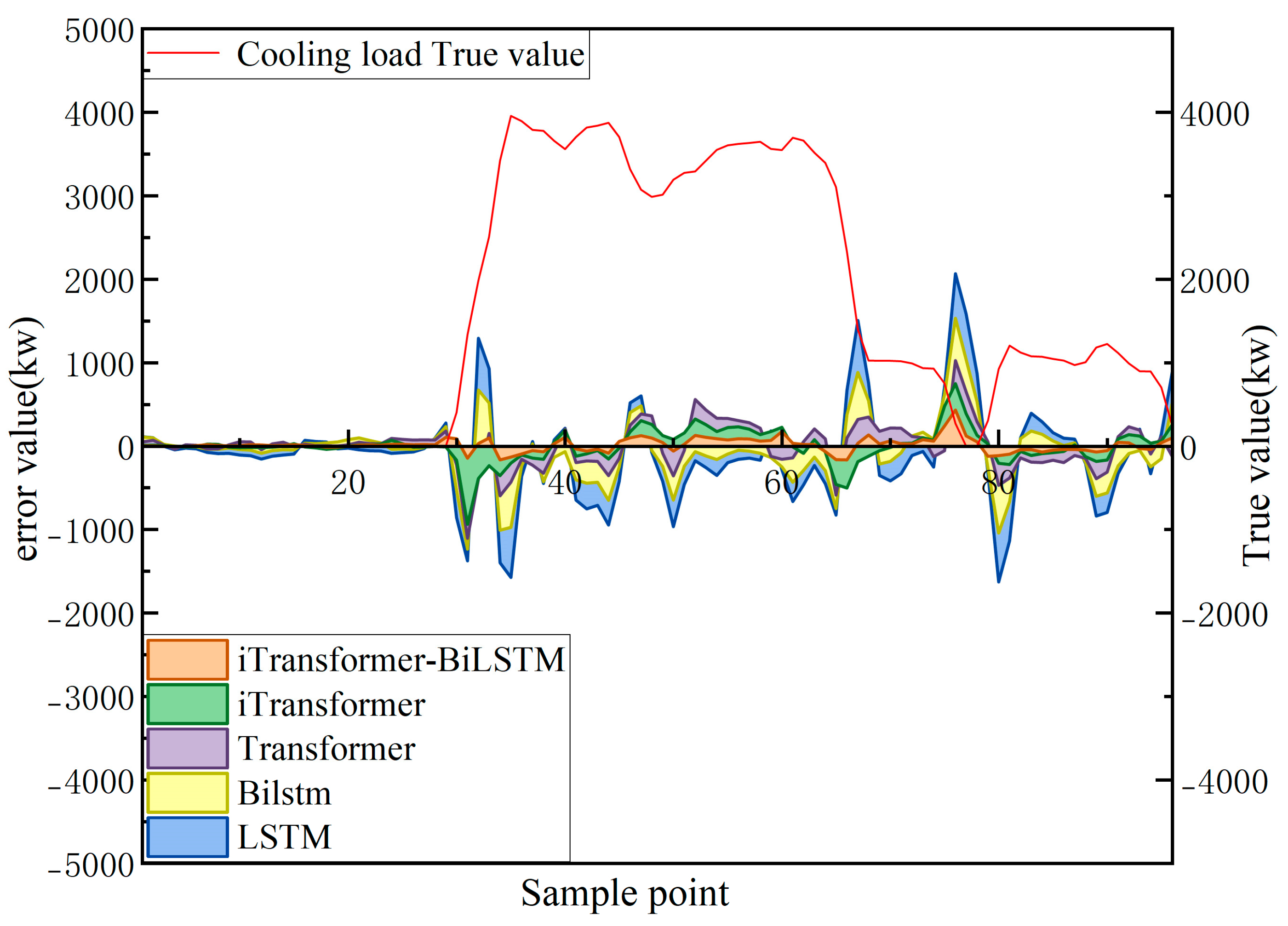
3.4.2. Comparative Analysis of Single Model

In order to verify the contribution of each module in the combined model, this paper designs a comparative experiment between the combined model (iTransformer-BiLSTM) and the single models (iTransformer, Transformer, BiLSTM, and LSTM). The main parameters of the sub-model are consistent with the main model, and the optimal results are obtained through multiple experiments (see

Table 4. Main model and single model prediction evaluation results.

Model	RMSE	MAE	SMAPE (%)
iTransformer-BiLSTM	93.963	62.788	4.936
iTransformer	135.271	81.733	5.953
Transformer	153.629	111.194	6.703
BiLSTM	196.028	134.015	8.799
LSTM	205.868	141.610	9.348

). The prediction curve and error distribution curve are shown in Figure 10, Figure 11 and Figure 12 (among them, the prediction curve takes 288 test data for three consecutive working days as the overall display, and the local prediction curve and error distribution take the first day data as the display).

The data presented in the table indicate that the iTransformer-BiLSTM hybrid model performs better than all standalone models across all evaluation metrics. Specifically, it achieves the lowest RMSE (93.963) and MAE (62.788) values, reducing RMSE and MAE by 30.5% and 23.2%, respectively, compared to the best-performing standalone model, iTransformer (RMSE: 135.271, MAE: 81.733). Furthermore, compared to BiLSTM (RMSE: 196.028, MAE: 134.015), the reductions are 52.1% and 53.3%, respectively, indicating that the hybrid model effectively integrates both global and local features to significantly reduce prediction errors.

Among standalone models, iTransformer (RMSE: 135.271, MAE: 81.733) outperforms the traditional Transformer (RMSE: 153.629, MAE: 111.194). This improvement is attributed to iTransformer’s independent token encoding strategy, which treats each variable’s entire time series as an independent input unit, thereby mitigating noise interference caused by variable coupling in traditional Transformers and enhancing the learning efficiency of multivariate time-series interactions. Additionally, BiLSTM (RMSE: 196.028) reduces the prediction error by 4.8% compared to LSTM (RMSE: 205.868), validating that the bidirectional propagation mechanism enhances the modeling of temporal dependencies by integrating historical and future contextual information.

In terms of error control, the iTransformer-BiLSTM model achieves the lowest SMAPE (4.936%) in the entire table, reducing SMAPE by 17.1% and 43.9% compared to iTransformer (5.953%) and BiLSTM (8.799%), respectively. This result indicates that the hybrid model maintains stable percentage error control even in highly fluctuating industrial scenarios. Although the standalone models exhibit strong error control capabilities, the hybrid model further enhances fine-grained fitting accuracy by utilizing a projection layer to align the scale of global features (e.g., the nonlinear interaction between outdoor humidity and supply-return air temperature difference) with local temporal dynamics (e.g., the sudden load drop during lunch breaks). This optimization enables superior performance under complex operating conditions. However, the computational complexity of the hybrid model is higher than that of individual models, necessitating a trade-off between accuracy improvement and hardware resource consumption in practical deployment. Experimental statistics show that the training time of the primary model, iTransformer-BiLSTM, is approximately 683 s, which is longer than that of iTransformer (442 s) and BiLSTM (57 s), indicating that the performance enhancement comes at the cost of increased computational overhead. In the future, engineering applicability could be further optimized through model lightweighting strategies.

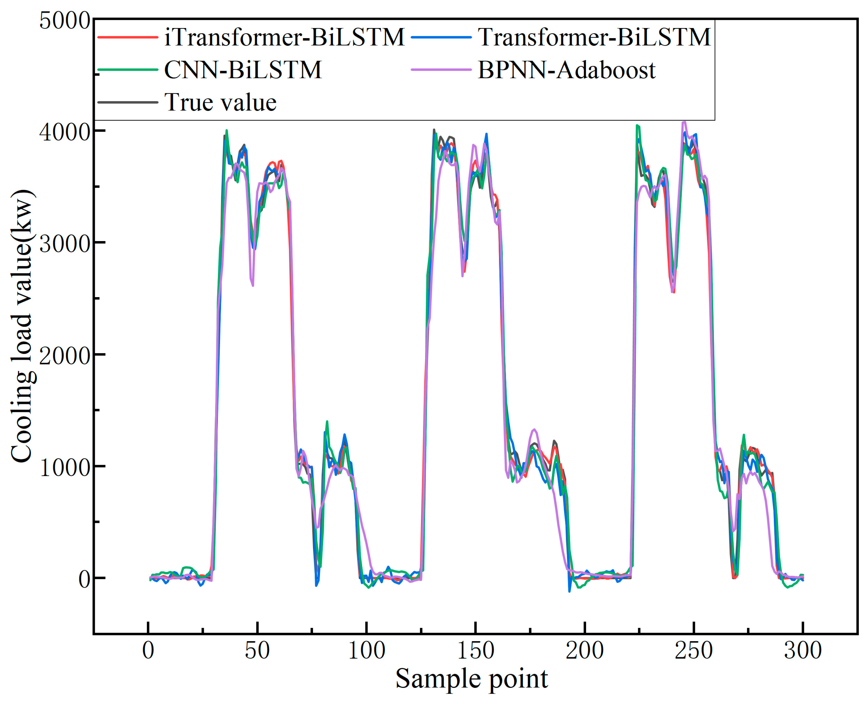
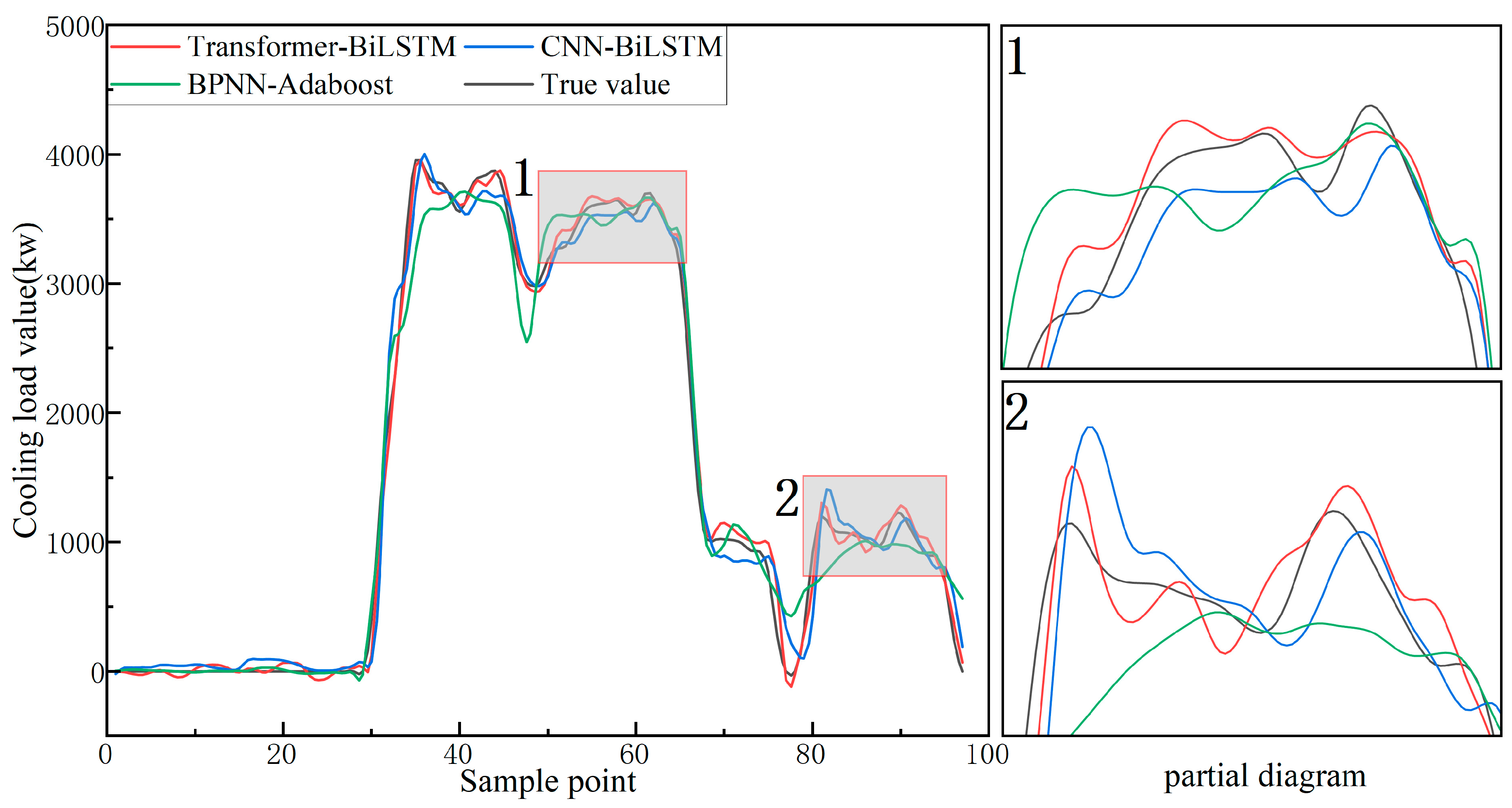
3.4.3. Comparative Analysis with Other Combined Models

To verify the scientific validity and effectiveness of the proposed iTransformer-BiLSTM hybrid model, this study conducted comparative experiments against mainstream load forecasting models, including BPNN-Adaboost, CNN-BiLSTM, and Transformer-BiLSTM, using the same test samples. The BPNN-Adaboost model, which combines traditional neural networks with ensemble algorithms, possesses a certain degree of nonlinear modeling capability [37,38]. The CNN-BiLSTM model integrates local feature extraction (CNN) with temporal sequence modeling (BiLSTM), achieving favorable performance in certain short-term load forecasting tasks [39,40]. The Transformer-BiLSTM model combines the global dependency learning capability of Transformer with the temporal dynamic analysis capability of BiLSTM, demonstrating strong performance in multi-step forecasting [41]. Therefore, these three hybrid models are selected as benchmarks for comparison, as they are structurally representative and align well with current research practices. The key parameter settings for each model are listed in

Table 5. Main Parameter Settings of Different Models.

Model	Main Parameter Settings
BPNN-Adaboost	Number of weak classifiers: 5, BPNN network layers: 2, Neurons per layer: 64/32
CNN-BiLSTM	CNN layers: 2, Kernel size: 2 × 2, Pooling layer size: 2 × 2, Channels: 128, BiLSTM settings: Same as the proposed main mode
Transformer-BiLSTM	Encoder layers: 2, Attention heads: 4, Channels: 128, BiLSTM settings: Same as the proposed main model

, and the optimal results were selected from multiple experiments to ensure experimental stability. The evaluation metrics of the prediction results, fitting curves, and error distributions are presented in

Table 6. Prediction Evaluation Results of the Main Model and Other Combined Models.

Model	RMSE	MAE	SMAPE (%)
iTransforme-BiLSTM	93.963	62.788	4.936
Transformer-BiLSTM	114.517	82.310	6.020
CNN-BiLSTM	174.387	116.031	8.574
BPNN-Adaboost	225.960	145.096	10.916

and Figure 13, Figure 14, and Figure 15, respectively.

The experimental results indicate that the iTransformer-BiLSTM model outperforms other benchmark models in terms of predictive performance. Compared to the Transformer-BiLSTM, CNN-BiLSTM, and BPNN-Adaboost models, its Root Mean Square Error (RMSE) is reduced by 20.554, 80.424, and 131.997, respectively. The Mean Absolute Error (MAE) decreases by 19.522, 53.243, and 82.308, while the Symmetric Mean Absolute Percentage Error (SMAPE) is lowered by 1.084%, 3.638%, and 5.980%, respectively. These results indicate that the iTransformer-BiLSTM model demonstrates better error control and predictive accuracy. For air conditioning systems in manufacturing facilities, a decrease in the SMAPE metric reflects enhanced cooling load prediction accuracy. This, in turn, facilitates more precise demand-driven cooling, mitigates energy waste associated with overcooling, and consequently improves both system operational efficiency and indoor thermal comfort.

Further examination of Figure 12 and Figure 15 reveals that the peak prediction errors are primarily concentrated during periods of significant fluctuations in the actual load, such as sudden surges and drops. This indicates that the magnitude of the errors is largely influenced by abrupt load variations. In contrast, traditional models exhibit insufficient responsiveness during such periods, leading to larger deviations. In comparison, the iTransformer-BiLSTM model, by integrating global variable features and temporal context dependencies, adapts more effectively to dynamic changes, resulting in minimized error fluctuations and a smoother overall prediction curve.

As a multivariate regression-based predictive model, BPNN-Adaboost relies on traditional regression mechanisms, making it less effective in capturing the dynamic characteristics of time series, which results in weaker predictive performance. Meanwhile, CNN-BiLSTM integrates a Convolutional Neural Network (CNN) for local feature extraction, enabling it to capture short-term temporal patterns. However, its limited receptive field restricts its ability to model long-term dependencies. Additionally, Transformer-BiLSTM leverages self-attention mechanisms to enhance long-sequence modeling, but its approach tends to overlook fine-grained interactions between variables, resulting in the need for improvement in prediction accuracy.

The proposed iTransformer-BiLSTM model enhances feature extraction capabilities by treating each variable as an independent token in iTransformer, thereby capturing inter-variable dependencies more effectively. By integrating BiLSTM, the model simultaneously leverages both local and global information, leading to superior performance in load forecasting tasks. This approach provides a more reliable technical foundation for load prediction and energy efficiency optimization in central air conditioning systems within manufacturing plants.

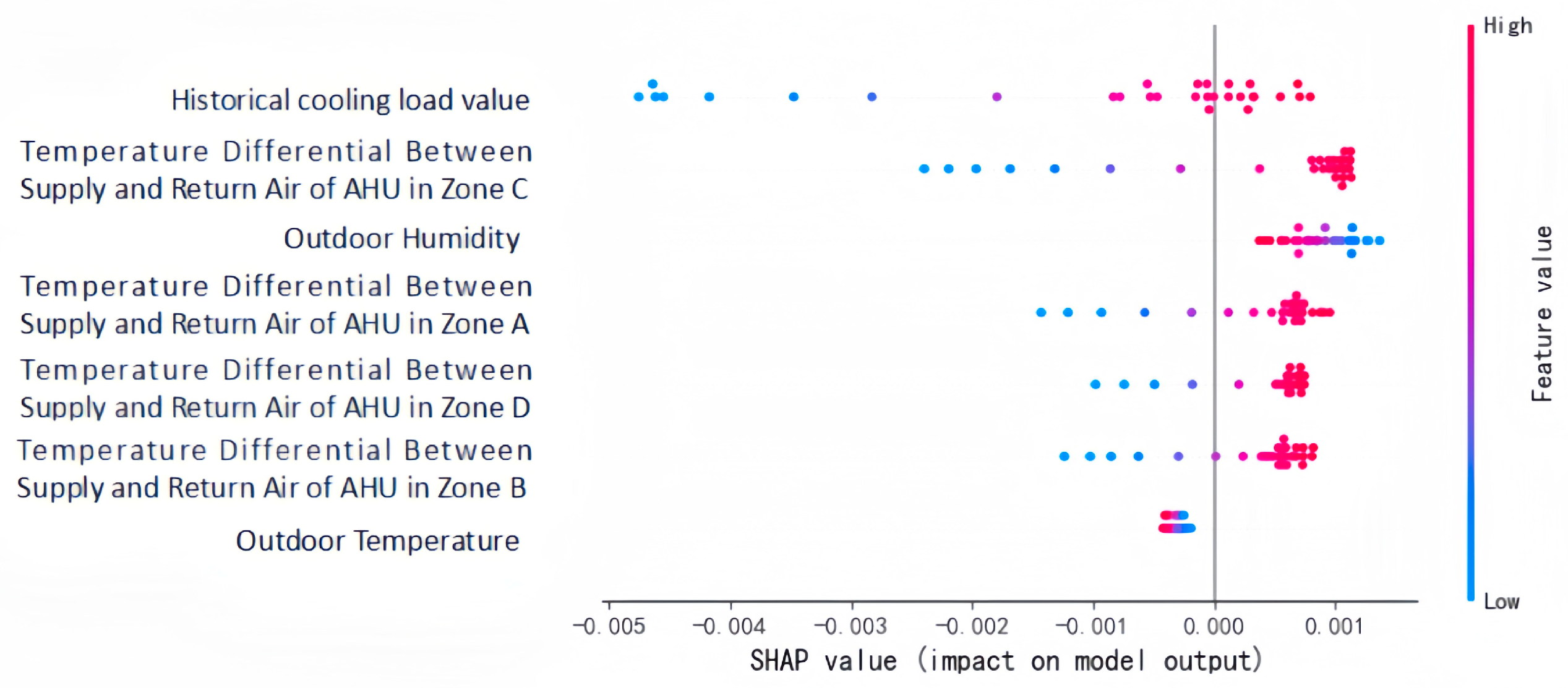
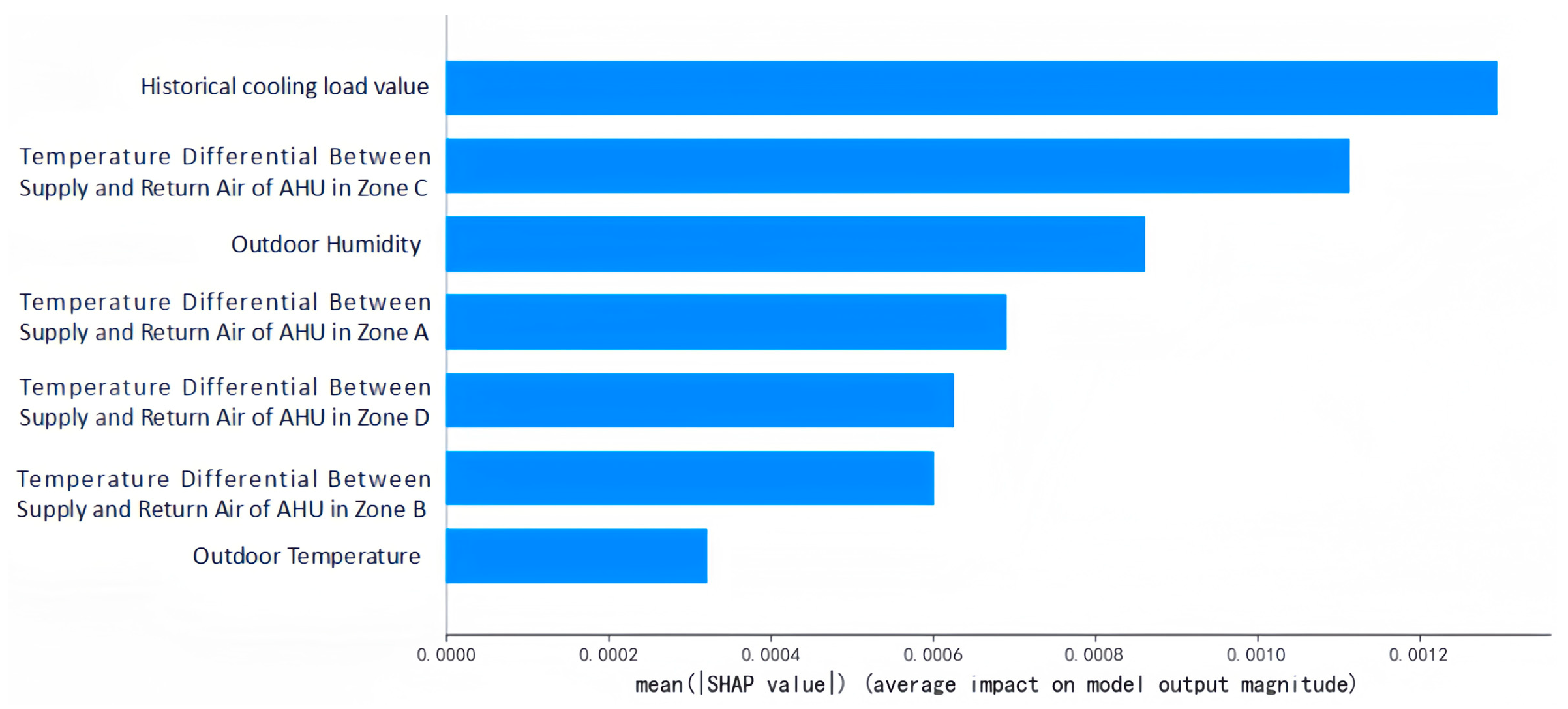
3.4.4. Model Input Variable Sensitivity Analysis

To further quantify the contribution of each input feature to the cooling load prediction results, this study conducted a sensitivity analysis of the iTransformer-BiLSTM model based on the SHAP (SHapley Additive exPlanations) method. Figure 16 shows the SHAP beeswarm plot of the features, while Figure 17 presents the bar chart of feature rankings based on the mean absolute SHAP values.

From the beeswarm plot (Figure 16), it can be observed that the SHAP values of the historical cooling load feature exhibit the widest distribution, with significant dispersion on both the positive and negative sides. This indicates that the historical cooling load exerts a bidirectional regulatory effect on the prediction output across different value ranges. Similarly, the temperature differences between supply and return air in Zones A, B, C, and D also display bidirectional dispersion, reflecting the dynamic response of indoor environmental parameters to cooling load fluctuations under different operating conditions. In contrast, the SHAP values of outdoor humidity are primarily concentrated on the positive side with a relatively narrow dispersion range, suggesting that it mainly provides a stable positive contribution. The SHAP values for outdoor temperature are relatively small and tightly clustered, indicating a minor influence on the prediction results.

The bar chart (Figure 17) further quantifies the average contribution level of each feature. Results show that historical cooling load accounts for the highest overall contribution and plays a dominant role. This is followed by the temperature difference between supply and return air in Zone C and outdoor humidity, suggesting that variations in Zone C air temperature and ambient humidity conditions are also important drivers of cooling load prediction. This is likely because Zone C, located in the central area of the factory workshop, more comprehensively represents the overall indoor cooling load variations, while the significance of outdoor humidity mainly stems from its direct impact on the latent heat load of the air-conditioning system—higher humidity levels during fresh air handling lead to greater cooling load demand.

Overall, the sensitivity analysis results indicate that the iTransformer-BiLSTM model can effectively identify the differences in feature contributions to cooling load prediction, demonstrating the model’s reasonable responsiveness to key variables under complex operating conditions.

4. Conclusions

To address the limitations of existing models in effectively capturing both inter-variable dependencies and temporal features of influencing factors in cooling load forecasting, which often result in insufficient prediction accuracy, this study proposes a hybrid forecasting approach based on iTransformer-BiLSTM. First, key indoor and outdoor influencing factors are identified through an in-depth analysis, and the iTransformer module is employed to extract features from the selected multivariate time-series data. By treating the entire time series as tokens and leveraging attention mechanisms, the model captures complex nonlinear relationships among variables. Subsequently, the extracted feature representations are fed into the BiLSTM module, which utilizes bidirectional long short-term memory mechanisms to model the bidirectional dynamic characteristics of the time series, thereby generating more precise load predictions. Experimental results demonstrate that, in the task of cooling load forecasting for industrial air conditioning systems, the proposed iTransformer-BiLSTM model outperforms both single and hybrid models in key evaluation metrics, including RMSE, MAE, and SMAPE, showcasing superior predictive performance and generalization capability. Meanwhile, sensitivity analysis of the input variables further validated the model’s capability to effectively identify the contribution relationships of key features in a multivariate environment, thereby enhancing the interpretability of the prediction results.

Nevertheless, the model’s actual performance is to some extent dependent on the relatively comprehensive sensor deployment and high data acquisition density currently available in the factory. The abundance of indoor and outdoor environmental data facilitates the model’s ability to fully learn the patterns of load variations. Therefore, under conditions of insufficient data coverage, sparse sensor layouts, or improperly positioned sensors, the prediction accuracy and stability may be adversely affected.

Future research could further incorporate real-time operational data to continuously optimize model parameters and introduce thermal analysis methods to systematically evaluate and optimize sensor placement and the types of monitoring data, thereby enhancing the scientific rigor of the data acquisition system and improving the quality of input features. On this basis, it is also necessary to further validate the scalability and adaptability of the model across industrial and commercial building environments of different scales and types, such as pharmaceutical workshops, shopping malls, and data centers, to enhance its engineering applicability across scenarios with varying cooling load characteristics.

References

1. Sun, L.; Hu, Z.; Mae, M.; Imaizumi, T. Deep transfer learning strategy based on TimesBlock-CDAN for predicting thermal environment and air conditioner energy consumption in residential buildings. Appl. Energy 2025, 381, 125188. [Google Scholar] [CrossRef]
2. Liu, J.; Zhai, Z.; Zhang, Y.; Wang, Y.; Ding, Y. Comparison of energy consumption prediction models for air conditioning at different time scales for large public buildings. J. Build. Eng. 2024, 96, 110423. [Google Scholar] [CrossRef]
3. Cen, J.; Zeng, L.; Liu, X.; Wang, F.; Deng, S.; Yu, Z.; Zhang, G.; Wang, W. Research on energy-saving optimization method for central air conditioning system based on multi-strategy improved sparrow search algorithm. Int. J. Refrig. 2024, 160, 263–274. [Google Scholar] [CrossRef]
4. Zhang, Q.; Tian, Z.; Ma, Z.; Li, G.; Lu, Y.; Niu, J. Development of the heating load prediction model for the residentia building of district heating based on model calibration. Energy 2020, 205, 117949. [Google Scholar] [CrossRef]
5. He, N.; Qian, C.; Liu, L.; Cheng, F. Air conditioning load prediction based on hybrid data decomposition and non-parametric fusion model. J. Build. Eng. 2023, 80, 108095. [Google Scholar] [CrossRef]
6. Roy, D.; Chakraborty, T.; Basu, D.; Bhattacharjee, B. Feasibility and performance of ground source heat pump systems for commercial applications in tropical and subtropical climates. Renew. Energy 2020, 152, 467–483. [Google Scholar] [CrossRef]
7. Cao, J.; Liu, J.; Man, X. A united WRF/TRNSYS method for estimating the heating/cooling load for the thousand-meter scale megatall buildings. Appl. Therm. Eng. 2017, 114, 196–210. [Google Scholar] [CrossRef]
8. Sangwan, P.; Mehdizadeh-Rad, H.; Ng, A.W.M.; Tariq, M.A.U.R.; Nnachi, R.C. Performance Evaluation of Phase Change Materials to Reduce the Cooling Load of Buildings in a Tropical Climate. Sustainability 2022, 14, 3171. [Google Scholar] [CrossRef]
9. Tao, Y.; Yan, H.; Gao, H.; Sun, Y.; Li, G. Applicaion of SVR optimized by modified simulated anneaing (MSA-SVR) air conditioning load prediction mode. J. Ind. Inf. Integr. 2019, 15, 247–251. [Google Scholar]
10. Cheng, R.; Yu, J.; Zhang, M.; Feng, C.; Zhang, W. Short-term hybrid forecasting model of ice storage air-conditioning based on improved SVR. J. Build. Eng. 2022, 50, 104194. [Google Scholar] [CrossRef]
11. Fan, C.; Liao, Y.; Zhou, G.; Zhou, X.; Ding, Y. Improving cooling load prediction reliability for HVAC system using Monte-Carlo simulation to deal with uncertainties in input variables. Energy Build. 2020, 226, 110372. [Google Scholar] [CrossRef]
12. Wang, Z.; Hong, T.; Piette, M.A. Building thermal load prediction through shallow machine learning and deep learning. Appl. Energy 2020, 263, 114683. [Google Scholar] [CrossRef]
13. Ahmad, T.; Chen, H.; Shair, J.; Xu, C. Deployment of data-mining short and medium-term horizon cooling load forecasting models for building energy optimization and management. Int. J. Refrig. 2019, 98, 399–409. [Google Scholar] [CrossRef]
14. Kwok, S.S.K.; Lee, E.W.M. A study of the importance of occupancy to building cooling load in prediction by intelligent approach. Energy Convers. Manag. 2011, 52, 2555–2564. [Google Scholar] [CrossRef]
15. Chao, W.H.; Dong, W. Prediction on hourly cooling load of buildings based on neural networks. Int. J. Smart Home 2015, 9, 35–52. [Google Scholar]
16. He, N.; Liu, L.; Qian, C.; Zhang, L.; Yang, Z.; Li, S. A closed-loop data-fusion framework for air conditioning load prediction based on LBF. Energy Rep. 2022, 8, 7724–7734. [Google Scholar] [CrossRef]
17. Sajjad, M.; Khan, Z.A.; Ullah, A.; Hussain, T.; Ullah, W.; Lee, M.Y.; Baik, S.W. A novel CNN-GRU-based hybrid approach for short-term residential load forecasting. IEEE Access 2020, 8, 143759–143768. [Google Scholar] [CrossRef]
18. Chen, J.; Ding, L.; Zhang, K.; Hou, C.; Lai, Z. Deep Learning Based Air Conditioning Set Temperature Prediction with Meteorological Data. In Proceedings of the 2023 IEEE Sustainable Power and Energy Conference (iSPEC), Chongqing, China, 28–30 November 2023; pp. 1–6. [Google Scholar]
19. Zhang, J.; Zhao, L. Efficient greenhouse gas prediction using IoT data streams and a CNN-BiLSTM-KAN model. Alex. Eng. J. 2025, 123, 261–270. [Google Scholar] [CrossRef]
20. Kavitha, R.J.; Thiagarajan, C.; Priya, P.I.; Anand, A.V.; Al-Ammar, E.A.; Santhamoorthy, M.; Chandramohan, P. Improved Harris Hawks Optimization with Hybrid Deep Learning Based Heating and Cooling Load Prediction on residential buildings. Chemosphere 2022, 309, 136525. [Google Scholar] [CrossRef]
21. Dosovitskiy, A.; Beyer, L.; Kolesnikov, A.; Weissenborn, D.; Zhai, X.; Unterthiner, T.; Dehghani, M.; Minderer, M.; Heigold, G.; Gelly, S.; et al. An image is worth 16x16 words: Transformers for image recognition at scale. arXiv 2020, arXiv:2010.11929. [Google Scholar]
22. Yuan, P.; Zhao, W.; Zhao, Y. Intelligent prediction algorithm of ship roll and pitch motion based on SSA-optimized BiLSTM network. Ocean Eng. 2025, 320, 120331. [Google Scholar] [CrossRef]
23. Vaswani, A.; Shazeer, N.; Parmar, N.; Uszkoreit, J.; Jones, L.; Gomez, A.N.; Kaiser, Ł.; Polosukhin, I. Attention is all you need. In Proceedings of the 31st International Conference on Neural Information Processing Systerms, Long Beach, CA, USA, 4–9 December 2017; Curran Associates Inc.: New York, NY, USA, 2017; pp. 6000–6010. [Google Scholar]
24. Yu, D.; Liu, T.; Wang, K.; Li, K.; Mercangöz, M.; Zhao, J.; Lei, Y.; Zhao, R. Transformer based day-ahead cooling load forecasting of hub airport air-conditioning systems with thermal energy storage. Energy Build. 2024, 308, 114008. [Google Scholar] [CrossRef]
25. Zou, Y.; Chen, Y.; Xu, Y.; Zhang, H.; Zhang, S. Short-term freeway traffic speed multistep prediction using an iTransformer model. Phys. A Stat. Mech. Its Appl. 2024, 655, 130185. [Google Scholar] [CrossRef]
26. Ren, D.; Hu, Q.; Zhang, T. EKLT: Kolmogorov-Arnold attention-driven LSTM with Transformer model for river water level prediction. J. Hydrol. 2025, 649, 132430. [Google Scholar] [CrossRef]
27. Li, W.; Liu, C.; Xu, Y.; Niu, C.; Li, R.; Li, M.; Hu, C.; Tian, L. An interpretable hybrid deep learning model for flood forecasting based on Transformer and LSTM. J. Hydrol. Reg. Stud. 2024, 54, 101873. [Google Scholar] [CrossRef]
28. Kow, P.Y.; Liou, J.Y.; Yang, M.T.; Lee, M.H.; Chang, L.C.; Chang, F.J. Advancing climate-resilient flood mitigation: Utilizing transformer-LSTM for water level forecasting at pumping stations. Sci. Total Environ. 2024, 927, 172246. [Google Scholar] [CrossRef]
29. Zhai, C.; He, X.; Cao, Z.; Abdou-Tankari, M.; Wang, Y.; Zhang, M. Photovoltaic power forecasting based on VMD-SSA-Transformer: Multidimensional analysis of dataset length, weather mutation and forecast accuracy. Energy 2025, 324, 135971. [Google Scholar] [CrossRef]
30. Wang, S.; Shi, J.; Yang, W.; Yin, Q. High and low frequency wind power prediction based on Transformer and BiGRU-Attention. Energy 2024, 288, 129753. [Google Scholar] [CrossRef]
31. Xue, H.; Wang, S.; Xia, M.; Guo, S. G-Trans: A hierarchical approach to vessel trajectory prediction with GRU-based transformer. Ocean Eng. 2024, 300, 117431. [Google Scholar] [CrossRef]
32. Lin, S.; Jiang, Y.; Hong, F.; Xu, L.; Huang, H.; Wang, B. HDFormer: A transformer-based model for fishing vessel trajectory prediction via multi-source data fusion. Ocean Eng. 2025, 320, 120309. [Google Scholar] [CrossRef]
33. Hochreiter, S.; Schmidhuber, J. Long Short-term Memory. Neural Comput. 1997, 9, 1735–1780. [Google Scholar] [CrossRef] [PubMed]
34. Zhou, H.; Zhang, S.; Peng, J.; Zhang, S.; Li, J.; Xiong, H.; Zhang, W. Informer: Beyond efficient transformer for long sequence time-series forecasting. In Proceedings of the AAAI Conference on Artificial Intelligence, Virtually, 19–21 May 2021; Volume 35, pp. 11106–11115. [Google Scholar]
35. Liu, Y.; Hu, T.; Zhang, H.; Wu, H.; Wang, S.; Ma, L.; Long, M. itransformer: Inverted transformers are effective for time series forecasting. arXiv 2023, arXiv:2310.06625. [Google Scholar]
36. Lai, T.C.; Xu, K.K.; Zhu, C.J.; Xu, K.K. A One-step Prediction Method of Building Cooling Load Based on Improved CNN-GRU. Mech. Electr. Eng. Technol. 2024, 53, 119–122. (In Chinese) [Google Scholar]
37. Ma, L.; Huang, Y.; Zhao, T. A synchronous prediction method for hourly energy consumption of abnormal monitoring branch based on the data-driven. Energy Build. 2022, 260, 111940. [Google Scholar] [CrossRef]
38. Fu, T. Short-term gas load forecasting based on BPAdaboost model. Sci. Technol. Bull. 2013, 29, 55–57. (In Chinese) [Google Scholar]
39. Luo, S.; Wang, B.; Gao, Q.; Wang, Y.; Pang, X. Stacking integration algorithm based on CNN-BiLSTM-Attention with XGBoost for short-term electricity load forecasting. Energy Rep. 2024, 12, 2676–2689. [Google Scholar] [CrossRef]
40. Su, Z.; Zheng, G.; Wang, G.; Hu, M.; Kong, L. An IDBO-optimized CNN-BiLSTM model for load forecasting in regional integrated energy systems. Comput. Electr. Eng. 2025, 123, 110013. [Google Scholar] [CrossRef]
41. Zhao, M.; Guo, G.; Fan, L.; Han, L.; Yu, Q.; Wang, Z. Short-term natural gas load forecasting analysis based on VMD-Transformer-BiLSTM. Appl. Integr. Circuits 2025, 42, 400–402. (In Chinese) [Google Scholar]
Figure 1. Structure of the LSTM Module.
Applsci 15 05214 g001
Figure 2. Structure of the BiLSTM Module.
Applsci 15 05214 g002
Figure 3. Structure of the iTransformer Module.
Applsci 15 05214 g003
Figure 4. Differences in Variable Time Series Embedding Methods between Transformer and iTransformer.
Applsci 15 05214 g004
Figure 5. Structure of the iTransformer-BiLSTM Model.
Applsci 15 05214 g005
Figure 6. Structure Diagram of the Chilled Water System.
Applsci 15 05214 g006
Figure 7. Distribution and Division of Temperature Points in the Factory Area.
Applsci 15 05214 g007
Figure 8. Changes in the Cooling Load of the Factory Workshop in June.
Applsci 15 05214 g008
Figure 9. Changes in the Cooling Load of the Factory Workshop within a Certain Week.
Applsci 15 05214 g009
Figure 10. Main model and single model comparison results (three days).
Applsci 15 05214 g010
Figure 11. Main model and single model comparison results and partial diagram (take the first day above).
Applsci 15 05214 g011
Figure 12. Comparison error analysis between the main model and the single model (take the first day above).
Applsci 15 05214 g012
Figure 13. Comparison Results between the Main Model and Other Combined Models (Three Days).
Applsci 15 05214 g013
Figure 14. Comparison Results between the Main Model and Other Combined Models and the Partial Diagram (Taking the First Day Mentioned Above).
Applsci 15 05214 g014
Figure 15. Error Analysis of the Comparison between the Main Model and Other Combined Models (Taking the First Day Mentioned Above).
Applsci 15 05214 g015
Figure 16. SHAP Beeswarm Plot of Input Features.
Applsci 15 05214 g016
Figure 17. Feature Ranking by Mean Absolute SHAP Values.
Applsci 15 05214 g017