Fault Estimation for Semi-Markov Jump Neural Networks Based on the Extended State Method

Abstract

This paper addresses fault estimation in discrete-time semi-Markov jump neural networks (s-MJNNs) under the Round-Robin protocol and proposes an innovative extended state observer-based approach. Unlike studies considering only constant transition rates, this work investigates s-MJNNs with time-varying transition probabilities, which more closely reflect practical situations. By incorporating actuator and sensor faults as augmented state variables, an extended state observer is proposed to estimate system states and faults simultaneously. To alleviate network congestion and optimize communication resources, the Round-Robin protocol is adopted to schedule data transmission efficiently. By constructing a Lyapunov–Krasovskii functional and applying the discrete Wirtinger inequality, sufficient conditions are derived to ensure the mean square exponential stability and dissipative performance of the system. The observer gain parameters are computed using the linear matrix inequality (LMI) method. Numerical simulations validate the effectiveness and performance of the proposed fault estimation method.

1. Introduction

With the rapid progress of science and technology, complex control systems have been widely used in computer-integrated manufacturing systems, network communication systems, agricultural machinery control systems, and modern agricultural flight control systems [1,2,3,4,5]. Furthermore, neural networks (NNs) have drawn extensive attention from both the academic field and the industrial and agricultural sectors in handling large-scale nonlinear systems. Nevertheless, these complex systems are frequently prone to unpredictable variations in their internal structure, such as equipment malfunctions, environmental alterations, disconnections of subsystems, information losses, and changes in interconnections among subsystems. Hence, how to improve the security and reliability of these systems has emerged as a crucial challenge.

Fortunately, the Markov process provides an effective framework for regulating such transitions. In practical applications, system modes can switch between different states at various time points, and these state transitions can be governed by a Markov chain. This characteristic has facilitated the development of Markov jump neural networks (MJNNs), which are recognized as one of the key classes of hybrid systems. In recent years, the development of dissipation has continued to improve, particularly the dissipation rate [6]. Scholars established a more general extended dissipation rate and applied it to continuous-time neural networks [7]. They studied the estimation of a reachable set based on an incomplete transition rate in discrete-time MJNNs. The research was further expanded to address the challenge of dissipative state estimation, considering finite piecewise-homogeneous Markov chains and mixed time delays [8]. Other scholars also studied the stochastic acceptability analysis of singular Markov jump delay systems (SMJDS) and designed a dissipative state estimator to deal with imperfect communication links [9]. It is worth noting that most Markov jump systems are constrained by a constant transition rate. However, in practice scenarios, the transition rate may not be constant and can instead be described by a semi-Markov process.

In practical applications, time delays are inevitable and often the primary cause of system instability, oscillations, and performance degradation. This issue is particularly pronounced in communication systems and networked control systems, where time delays are inherently random and time-varying. Consequently, time-varying delays are typically modeled using probabilistic approaches [10,11,12]. Nonetheless, research on discrete-time semi-Markov jump neural networks(s-MJNNs) with time delays remains relatively scarce, further motivating our exploration of this topic. In state estimation studies for neural networks, it is commonly assumed that adequate communication protocols are in place between sensors and the state estimator, ensuring synchronization and data transmission from all sensors at each sampling interval. Three communication protocols are commonly used in control systems: the Round-Robin protocol (RRP), the Weighted Try-Once-Discard protocol (WTODP), and the Stochastic Communication protocol (SCP) [13,14,15,16]. Among these, RRP-based state estimation methods have been extensively studied due to their structured scheduling and efficient resource allocation. To improve communication efficiency and alleviate network congestion, RRP is adopted to schedule sensor data transmission in a cyclic and fair manner, ensuring a balanced network load and minimizing data loss. Compared to SCP and WTODP, RRP provides deterministic scheduling, preventing data starvation in critical sensors and enhancing the accuracy of real-time fault estimation. Furthermore, by integrating RRP into the observer design, the proposed method ensures a stable and systematic sensor data transmission strategy, thereby improving estimation performance under constrained communication bandwidth. Zou [17] proposed an RRP scheme incorporating random perturbations to address the state estimation problem in dynamic networks under random noise conditions. In addition, the research shows that the event-triggered strategy and non-fragile controller design can realize the dissipative synchronization problem of MJNNs with inertial terms [18,19]. Although numerous studies on discrete-time NN state estimation exist in the literatures [20,21,22,23], Li proposed a state estimation approach for MJNNs with mixed delays to guarantee that the resulting error system exhibits extended stochastic dissipativity [24]. The study of using RRP to deal with the problem of discrete-time s-MJNN observers has not been fully developed, which is one of the important motives for our research.

In recent years, many researchers have achieved significant advancements in the field of fault diagnosis. Example, the extended state approach is utilized to address the issue of fault detection in discrete systems, while the singular system method is used to solve the H∞ fault detection problem of mixed models [25]. Other researchers have proposed fault detection methods for Markov jump systems and designed observers capable of simultaneously estimating actuator faults, sensor faults, and system states [26,27,28]. Additionally, new observer design methods have been introduced for switched fuzzy stochastic systems with sensor and actuator faults, enabling the simultaneous estimation of system states and faults [29,30]. Although some scholars have investigated communication protocols in discrete-time s-MJNNs and others have focused on fault estimation in Markov jump systems, no existing research has addressed fault estimation in discrete-time s-MJNNs while simultaneously considering both communication constraints and delays using a novel extended state method. Therefore, it is necessary to investigate fault estimation in s-MJNNs based on the extended state method, which carries significant theoretical and practical implications.

Based on the above background, our research focuses on the fault estimation problem for discrete-time s-MJNNs with time delays. To achieve an “average” distribution of data transmission among sensors, a scheduling scheme based on the RRP is studied in this paper. The main innovations of this paper are as follows:

(1)

A novel state augmentation approach is proposed, incorporating sensor faults into the system as augmented state variables.

(2)

To avoid data congestion and save communication resources, the RRP scheme is adopted to schedule sensor data transmission.

(3)

A discrete-time extended state observer is designed to simultaneously estimate system states, actuator faults, and sensor faults under time-varying delay conditions.

(4)

Triple summation terms are introduced into the Lyapunov function, and their forward differences are bounded using the reciprocal convexity method, ensuring that the error system exhibits enhanced stochastic dissipativity.

2. Preliminaries

The following class of discrete-time s-MJNNs with time-varying delay is considered in the below form:

$$\begin{array}{cc}\hfill x(g+ 1) =& A(r(g))x(g) +B(r(g))f(x(g)) +C(r(g))f(x(g-d(g)))\hfill \\ & +D(r(g))\omega (g)+H(r(g))fa(g)\hfill \\ \hfill y(g)=& E(r(g))x(g)+G(r(g))fs(g)\hfill \\ \hfill z(g)=& F(r(g))x(g))\hfill \\ \hfill x(g)=& \overline{x}(g),g=-d_2,-d_2+1,\dots ,0,\hfill \end{array}$$

(1)

where $fa(g)$ is the actuator fault; $fs(g)$ is the sensor fault; $x(g)\in R^l$ and $y(g)\in R^n$ represent the neural state vector and the measurement output, respectively; $z(g)\in R^m$ is the estimated output signal, and $\omega (g)\in R^w$ denotes an external disturbance constrained within the range $\left[0,\infty \right]$. $A(r(g))=diag(a_1(r(g)),\dots .,a_n(r(g)))$ is the positive diagonal matrix. $B(r(g))$, $C(r(g))$, and $D(r(g))$ represent the known weight matrices. $R^l$, $R^n$, and $R^w$ denote the $l$-dimensional, $n$-dimensional, and $w$-dimensional real vector spaces, respectively. $f(x(g))={\left[f_1(x_1(g)),f_2(x_2(g)), f_3(x_3(g)),. . . ,f_n{x}_n(g))\right]}^T\in R^n$ is the neural activation function. $E(r(g))$, $F(r(g))$ is the interconnection weight matrices. $H(r(g))$ represents the fault influence matrix, which characterizes how actuator faults affect the system state. $G(r(g))$ is the sensor fault influence matrix, describing how sensor faults alter the measured output. $d(g)$ is marked by the time-varying delay and satisfies $d_1\le (g)\le d_2$, where $d_1$ and $d_2$ are the upper and lower bounds of the time delay. The parameter $r(g),g>0$ represents a semi-Markov chain, whose evolution is governed as follows:

$$P\left\{r(g+\zeta )=q|r(g)=p\right\}=\left\{\begin{array}{l}{\pi }_{pq}(\zeta )\chi +o(\zeta ), if p\ne q,\\ 1+{\pi }_{pp}(\zeta )\chi +o(\zeta ),if p=q,\end{array}\right\}$$

where $\zeta >0$ is the sojourn time. $li{m}_{\zeta \to 0}(o(\zeta )/\zeta )=0$ and ${\pi }_{pq}(\zeta )\ge 0$ for $p\ne q$ are the transition rates from mode $i$ at time $g$ to mode $q$ at time $g+\chi$ and ${\pi }_{pq}(\chi )=-{\displaystyle {\sum }_{q=1,q=p}^Q{\pi }_{pq}(\chi )}$.

Remark 1.

This study considers that faults and disturbances within the system are distinct, with disturbances being constrained within certain bounds.

Considering the limited bandwidth of communication channels from sensors to the observer, data congestion and other similar issues may arise. To address these challenges, this paper introduces the RRP approach to alleviate network congestion. Let ${\tilde{y}}_{\mathcal{l}}(g)=(\mathcal{l}\in 1,2,3,. . . ,m)$ represent the measurement output received from the $\mathcal{l}$th sensor. Following the RRP, ${\tilde{y}}_{\mathcal{l}}(g)$ can take the following form:

$${\tilde{y}}_{\mathcal{l}}(g)=\left\{\begin{array}{cc}{y}_{\mathcal{l}}(g),& \mathrm{if} \mathrm{mod}(g-\mathcal{l}, m)=0,\\ {\tilde{y}}_{\mathcal{l}}(g-1),& \mathrm{other}.\end{array}\right.$$

(2)

In accordance with (2), it can be reformulated as follows:

$$\tilde{y}(g)={\psi }_{\sigma }(g)y(g)+(I-{\psi }_{\sigma }(g))\tilde{y}(g-1),$$

(3)

where $y(g)={\left[{y_1}^T(g),{y_2}^T(g),\dots ,{y_m}^T(g)\right]}^T$, $\tilde{y}(g)={\left[{{\tilde{y}}_1}^T(g),{{\tilde{y}}_2}^T(g),\dots ,{{\tilde{y}}_m}^T(g)\right]}^T$, $\sigma (g)=mod(g-\mathcal{l},m)+1$, and ${\psi }_{\sigma (g)}=diag\left\{\tau (\sigma (g)-1)I,\tau (\sigma (g)-2)I,..,\tau (\sigma (g)-m)I\right\}$ with $\tau (·)\in \left\{0,1\right\}$ is the Kronecker delta function. To simplify the notation, $r(g)$ is represented by $p$. The incorporating the RRP is reformulated as follows:

$$\begin{array}{cc}\hfill \overline{x}(g+1)=& {\overline{\mathcal{A}}}_{p,\sigma (g)}\overline{x}(g)+{\overline{\mathcal{B}}}_{p}f(\overline{x}(g))+{\overline{\mathcal{C}}}_{p}f(\overline{x}(g-d(g)))+{\overline{\mathcal{D}}}_p\overline{\omega }(g)+{\overline{\mathcal{H}}}_{p}fa(g),\hfill \\ \hfill \overline{y}(g)=& {\overline{\mathcal{E}}}_{p,\sigma (g)}\overline{x}(g)+{\overline{\mathcal{G}}}_{p}fs(g), \hfill \\ \hfill \overline{z}(g)=& {\overline{\mathcal{F}}}_{p}x(g),\hfill \end{array}$$

(4)

where $\overline{y}$ is the measurement output after joining the RRP, $\overline{x}$ is the state vector after joining the RRP, $\overline{z}$ is the output with estimation after joining the RRP. $\overline{x}(g)=\left[\begin{array}{c}x\\ \tilde{y}(g-1)\end{array}\right]$, $\overline{\omega }(g)=\left[\begin{array}{c}\omega \\ 0\end{array}\right]$, $f(\overline{x}(g))=\left[\begin{array}{c}f(x(g))\\ 0\end{array}\right]$, ${\overline{\mathcal{A}}}_{p,\sigma (g)}=\left[\begin{array}{cc}{A}_p& 0\\ {\psi }_{\sigma (g)}{E}_p& I-{\psi }_{\sigma (g)}\end{array}\right]$, ${\overline{\mathcal{B}}}_p=\left[\begin{array}{cc}{B}_p& 0\\ 0& B_p\end{array}\right]$, ${\overline{\mathcal{C}}}_p=\left[\begin{array}{cc}{C}_p& 0\\ 0& C_p\end{array}\right]$, ${\overline{\mathcal{D}}}_p=\left[\begin{array}{cc}{D}_p& 0\\ 0& D_p\end{array}\right]$, ${\overline{\mathcal{E}}}_{p,\sigma (g)}=\left[\begin{array}{cc}{\psi }_{\sigma (g)}{E}_p& I-{\psi }_{\sigma (g)}\end{array}\right]$, ${\overline{\mathcal{G}}}_p=\left[\begin{array}{cc}{G}_p& 0\\ 0& G_p\end{array}\right]$, ${\overline{\mathcal{H}}}_p=\left[\begin{array}{cc}{H}_p& 0\\ 0& H_p\end{array}\right]$, ${\overline{\mathcal{F}}}_p=\left[\begin{array}{cc}{F}_p& 0\end{array}\right]$.

By utilizing the extended state method, an observer is constructed to effectively and accurately estimate both the system states and faults. Set $\overrightarrow{x}(g)=\left[\begin{array}{c}\overline{x}(g)\\ fs(g)\end{array}\right]$. Then, the extended equation is (5), as follows:

$${\overrightarrow{E}}_0\overrightarrow{x}(g+1)={\overrightarrow{\mathcal{A}}}_{p,\sigma (g)}\overrightarrow{x}(g)+{\overrightarrow{\mathcal{B}}}_{p}f(\overrightarrow{x}(g))+{\overrightarrow{\mathcal{C}}}_{p}f(\overrightarrow{x}(g-d(g)))+{\overrightarrow{\mathcal{D}}}_p\overline{\omega }(g)+{\overrightarrow{\mathcal{H}}}_{p}fa(g)+{\overrightarrow{\mathcal{G}}}_{p}fs(g)$$

(5)

where ${\overrightarrow{E}}_0=\left[\begin{array}{cc}I& 0\\ 0& 0\end{array}\right]$, ${\overrightarrow{\mathcal{A}}}_{p,\sigma (g)}=\left[\begin{array}{cc}{\overline{\mathcal{A}}}_{p,\sigma (g)}& 0\\ 0& -{\overline{\mathcal{G}}}_p\end{array}\right]$, ${\overrightarrow{\mathcal{B}}}_{p,\sigma (g)}=\left[\begin{array}{cc} {\overline{\mathcal{B}}}_p& 0\end{array}\right]$, ${\overrightarrow{\mathcal{C}}}_{p,\sigma (g)}=\left[\begin{array}{cc}{\overline{\mathcal{C}}}_p& 0\end{array}\right]$, ${\overrightarrow{\mathcal{D}}}_{p,\sigma (g)}=\left[\begin{array}{cc}{\overline{\mathcal{D}}}_p& 0\end{array}\right]$, ${\overrightarrow{\mathcal{H}}}_p=\left[\begin{array}{cc}{\overline{\mathcal{H}}}_p& 0\end{array}\right]$, ${\overrightarrow{\mathcal{G}}}_p=\left[\begin{array}{cc}0& {\overline{\mathcal{G}}}_p\end{array}\right]$.

The corresponding $\overrightarrow{y}(g)$ and $\overrightarrow{z}(g)$ in Equation (4) can be transformed into Equation (6):

$$\begin{array}{cc}\hfill \overline{y}(g)& ={\overline{\mathcal{E}}}_{p,\sigma (g)}\overline{x}(g)+ {\overline{\mathcal{G}}}_{p}fs(g)\hfill \\ & ={\overrightarrow{\mathcal{E}}}_{p0,\sigma (g)}\overrightarrow{x}(g)\hfill \\ & ={\overrightarrow{\mathcal{E}}}_{p,\sigma (g)}\overrightarrow{x}(g)+ {\overline{\mathcal{G}}}_{p}fs(g), \hfill \\ \hfill \overline{z}(g)& ={\overrightarrow{\mathcal{F}}}_p\overrightarrow{x}(g),\hfill \end{array}$$

(6)

Then, we have (7):

$${\overline{\mathcal{G}}}_{p}fs(g)=\overline{y}(g)-{\overrightarrow{\mathcal{E}}}_{p,\sigma (g)}\overrightarrow{x}(g),$$

(7)

where $f(\overrightarrow{x}(g))=f(\left[\begin{array}{l}\overline{x}(g)\\ fs(g)\end{array}\right])$, ${\overrightarrow{\mathcal{E}}}_{p0,\sigma (g)}=\left[\begin{array}{cc}I& 0\\ 0& I\end{array}\right]$, ${\overrightarrow{\mathcal{E}}}_{p,\sigma (g)}=\left[\begin{array}{cc}{\overline{\mathcal{E}}}_{p,\sigma (g)}& 0\end{array}\right]$, ${\overrightarrow{\mathcal{F}}}_p=\left[\begin{array}{cc}{\overline{\mathcal{F}}}_p & 0\end{array}\right]$.

Set ${\overrightarrow{I}}_1=\left[\begin{array}{c}0\\ I\end{array}\right]$. Combining it with Equation (5), Equation (8) is obtained as follows:

$$\begin{array}{ll}{\overrightarrow{E}}_0\overrightarrow{x}(g+1) \hfill & \hfill = {\overrightarrow{\mathcal{A}}}_{p,\sigma (g)}\overrightarrow{x}(g)+{\overrightarrow{\mathcal{B}}}_{p}f(\overrightarrow{x}(g)) +{\overrightarrow{\mathcal{C}}}_{p}f(\overrightarrow{x}(g-d(g))) + {\overrightarrow{\mathcal{D}}}_p\overline{\omega }(g)\\ & +{\overrightarrow{\mathcal{H}}}_{p}fa(g)+{\overrightarrow{I}}_1\overline{y}(g)-{\overrightarrow{I}}_1{\overrightarrow{\mathcal{E}}}_{p,\sigma (g)}\overrightarrow{x}(g)\hfill \end{array}$$

(8)

Set ${\overrightarrow{\overrightarrow{\mathcal{A}}}}_{p,\sigma (g)}={\overrightarrow{\mathcal{A}}}_{p,\sigma (g)}-{\overrightarrow{\mathcal{E}}}_{p,\sigma (g)}$, according to Equation (8), to obtain the following Equation (9):

$$\begin{array}{cc}\hfill {\overrightarrow{E}}_0\overrightarrow{x}(g+1)& ={\overrightarrow{\overrightarrow{\mathcal{A}}}}_{p,\sigma (g)}\overrightarrow{x}(g)+{\overrightarrow{\mathcal{B}}}_{p}f(\overrightarrow{x}(g))+{\overrightarrow{\mathcal{C}}}_{p}f(\overrightarrow{x}(g-d(g)))+{\overrightarrow{\mathcal{D}}}_p\overline{\omega }(g)\hfill \\ & +{\overrightarrow{\mathcal{H}}}_{p}fa(g)+{\overrightarrow{I}}_1\overline{y}(g)\hfill \end{array}$$

(9)

Set $\overrightarrow{M}=\left[\begin{array}{c}0\\ M_0\end{array}\right]$, where $M_0$ is an invertible matrix, adding $\overrightarrow{M}\left[\begin{array}{cc}{\overline{\mathcal{E}}}_{p,\sigma (g)}& {\overline{\mathcal{G}}}_p\end{array}\right]\overrightarrow{x}(g+1)$ to both sides of Equation (9), which yields Equation (10):

$$\begin{array}{ll}\hfill {\overrightarrow{E}}_1\overrightarrow{x}(g+1)& ={\overrightarrow{\overrightarrow{\mathcal{A}}}}_{p,\sigma (g)}\overrightarrow{x}(g)+{\overrightarrow{\mathcal{B}}}_{p}f(\overrightarrow{x}(g)) + {\overrightarrow{\mathcal{C}}}_{p}f(\overrightarrow{x}(g-d(g)))+{\overrightarrow{\mathcal{D}}}_p\overline{\omega }(g)\hfill \\ & +{\overrightarrow{\mathcal{H}}}_{p}fa(g) +{\overrightarrow{I}}_1\overline{y}(g)+\overrightarrow{M}\left[\begin{array}{cc}{\overline{\mathcal{E}}}_{p,\sigma (g)}& {\overline{\mathcal{G}}}_p\end{array}\right]\overrightarrow{x}(g+1)\hfill \end{array}$$

(10)

where ${\overrightarrow{E}}_1={\overrightarrow{E}}_0+\overrightarrow{M}\left[{\overline{\mathcal{E}}}_{p,\sigma (g)}{\overline{\mathcal{G}}}_p\right]=\left[\begin{array}{cc}I& 0\\ M_0{\overline{\mathcal{E}}}_{p,\sigma (g)}& M_0{\overline{\mathcal{G}}}_p\end{array}\right]$.

Set ${\overrightarrow{E}}_2=\left[\begin{array}{cc}I& 0\\ -{{\overline{\mathcal{G}}}_p}^{-1}{\overline{\mathcal{E}}}_{p,\sigma (g)}& -{{\overline{\mathcal{G}}}_p}^{-1}{M_0}^{-1}\end{array}\right]$ and ${\overrightarrow{E}}_1{\overrightarrow{E}}_2=1$, and derive (12) from (11):

$$\begin{array}{ll}\hfill \overrightarrow{x}(g+1)& ={\overrightarrow{E}}_2{\overrightarrow{\overrightarrow{\mathcal{A}}}}_{p,\sigma (g)}\overrightarrow{x}(g)+{\overrightarrow{E}}_2{\overrightarrow{\mathcal{B}}}_{p}f(\overrightarrow{x}(g))+{\overrightarrow{E}}_2{\overrightarrow{\mathcal{C}}}_{p}f(\overrightarrow{x}(g-d(g)))+{\overrightarrow{E}}_2{\overrightarrow{\mathcal{D}}}_p\overline{\omega }(g) \hfill \\ & +{\overrightarrow{E}}_2{\overrightarrow{\mathcal{H}}}_{p}fa(g)+{\overrightarrow{E}}_2{\overrightarrow{I}}_1\overline{y}(g)+{\overrightarrow{E}}_2\overrightarrow{M}\left[{\overline{\mathcal{E}}}_{p,\sigma (g)}{\overline{\mathcal{G}}}_p\right]\overrightarrow{x}(g+1)\hfill \end{array}$$

(11)

From Equation (4), Equation (12) can be obtained:

$$\left[\begin{array}{cc}{\overline{\mathcal{E}}}_{p,\sigma (g)}& {\overline{\mathcal{G}}}_p\end{array}\right]\overrightarrow{x}(g)=\overline{y}(g)$$

(12)

Then, Equation (13) is obtained based on Equations (11) and (12):

$$\begin{array}{ll}\hfill \overrightarrow{x}(g+1)& ={\overrightarrow{E}}_2{\overrightarrow{\overrightarrow{\mathcal{A}}}}_{p,\sigma (g)}\overrightarrow{x}(g)+{\overrightarrow{E}}_2{\overrightarrow{\mathcal{B}}}_{p}f(\overrightarrow{x}(g))+{\overrightarrow{E}}_2{\overrightarrow{\mathcal{C}}}_{p}f(\overrightarrow{x}(g-d(g)))+{\overrightarrow{E}}_2{\overrightarrow{\mathcal{D}}}_p\overline{\omega }(g)\hfill \\ & +{\overrightarrow{E}}_2{\overrightarrow{\mathcal{H}}}_{p}fa(g)+{\overrightarrow{E}}_2{\overrightarrow{I}}_1\overline{y}(g)+{\overrightarrow{E}}_2\overrightarrow{M}\overline{y}(g+1)\hfill \end{array}$$

(13)

Set $\mathcal{Z}(g)=\overrightarrow{x}(g)-{\overrightarrow{E}}_2\overrightarrow{M}\overline{y}(g)$ to obtain (14):

$$\begin{array}{ll}\hfill \mathcal{Z}(g+1)& ={\overrightarrow{E}}_2{\overrightarrow{\overrightarrow{\mathcal{A}}}}_{p,\sigma (g)}\mathcal{Z}(g)+{\overrightarrow{E}}_2{\overrightarrow{\mathcal{B}}}_{p}f(\mathcal{Z}(g)+{\overrightarrow{E}}_2\overrightarrow{M}\overline{y}(g))+{\overrightarrow{E}}_2{\overrightarrow{\mathcal{C}}}_{p}f(\mathcal{Z}(g-d(g))\hfill \\ & +{\overrightarrow{E}}_2\overrightarrow{M}\overline{y}(g-d(g)))+{\overrightarrow{E}}_2{\overrightarrow{\mathcal{D}}}_p\overline{\omega }(g)+{\overrightarrow{E}}_2{\overrightarrow{\mathcal{H}}}_{p}fa(g)+\overrightarrow{\mathcal{I}}\overline{y}(g)\hfill \end{array}$$

(14)

where $\overrightarrow{\mathcal{I}}={\overrightarrow{E}}_2{\overrightarrow{I}}_1$. The fault estimator observer is designed as shown in Equations (15)–(19). Based on the extended state method, it enables the simultaneous estimation of system states and faults, improving fault estimator accuracy.

$$\begin{array}{ll}\hfill \widehat{\mathcal{Z}}(g+1)& ={\overrightarrow{E}}_2{\overrightarrow{\overrightarrow{\mathcal{A}}}}_{p,\sigma (g)}\widehat{\mathcal{Z}}(g)+{\overrightarrow{E}}_2{\overrightarrow{\mathcal{B}}}_{p}f(\widehat{\mathcal{Z}}(g)+{\overrightarrow{E}}_2\overrightarrow{M}\overline{y}(g))+{\overrightarrow{E}}_2{\overrightarrow{\mathcal{C}}}_{p}f(\widehat{\mathcal{Z}}(g-d(g))\hfill \\ & +{\overrightarrow{E}}_2\overrightarrow{M}\overline{y}(g-d(g)))+{\overrightarrow{E}}_2{\overrightarrow{\mathcal{H}}}_p\widehat{f}a(g)+\overrightarrow{\mathcal{I}}\overline{y}(g)+{\overrightarrow{\mathcal{K}}}_{p,\sigma (g)}(\overline{y}(g)-\widehat{\overline{y}}(g))\hfill \end{array}$$

(15)

$$\widehat{\overline{y}}(g)={\overrightarrow{\mathcal{E}}}_{p0,\sigma (g)}\widehat{\overrightarrow{x}}(g)$$

(16)

$$\widehat{z}(g)={\overrightarrow{\mathcal{F}}}_p\widehat{\overrightarrow{x}}(g)$$

(17)

$$\widehat{\overrightarrow{x}}(g)=\widehat{\mathcal{Z}}(g)+{\overrightarrow{E}}_2\overrightarrow{M}\overline{y}(g)$$

(18)

$$\begin{array}{c}\widehat{f}a(g)=\mathcal{L}-{\mathcal{K}}_3(\overline{y}(g)-\widehat{\overline{y}}(g))\\ \mathcal{L}(g+1)={\overrightarrow{\mathcal{K}}}_{pp,\sigma (g)}(\overline{y}(g)-\widehat{\overline{y}}(g))\end{array}$$

(19)

where $\widehat{\overrightarrow{x}}(g)$ and $\widehat{\overline{y}}(g)$ represent the estimated vectors of $\overrightarrow{x}(g)$ and $\overline{y}(g)$, respectively. $\widehat{z}(g)$ is the estimated of $z(g)$. $\widehat{\mathcal{Z}}(g)$ is the estimated vector of $\mathcal{Z}(g)$. $\widehat{f}a(g)$ is the estimated vector of $fa(g)$. Matrices ${\overrightarrow{\mathcal{K}}}_{p,\sigma (g)}={\left[\begin{array}{cc}{\overrightarrow{\mathcal{K}}}_{p1,\sigma (g)}& {\overrightarrow{\mathcal{K}}}_{p2,\sigma (g)}\end{array}\right]}^{\mathrm{T}}$ and ${\overrightarrow{\mathcal{K}}}_{pp,\sigma (g)}$ are gain parameters to be determined for the fault estimation process, ensuring accurate estimation convergence. Matrix ${\mathcal{K}}_3$ is an adjustable parameter used to fine-tune the fault estimation performance.

Fault estimates play a key role in accurately identifying actuator and sensor faults, ensuring the reliability of the proposed estimation framework. Therefore, the estimator must be designed to minimize errors and ensure convergence to actual fault values. According to Equations (18) and (19), the fault estimates are given by

$$\begin{array}{cc}\hfill fa(g+1)& =\mathcal{L}(g+1)+{\mathcal{K}}_3(\overline{y}(g)-\widehat{\overline{y}}(g\left)\right)\hfill \\ & ={\overrightarrow{\mathcal{K}}}_{pp,\sigma (g)}(\overline{y}(g)-\widehat{\overline{y}}(g))+{\mathcal{K}}_3(\overline{y}(g+1)-\widehat{\overline{y}}(g+1))\hfill \end{array}$$

(20)

Set $\tilde{\mathcal{Z}}(g)=\mathcal{Z}(g)-\widehat{\mathcal{Z}}(g)$ and $\tilde{f}a(g)=fa(g)-\widehat{f}a(g)$. Then, we have an estimation error of Equation (21):

$$\begin{array}{cc}\hfill \tilde{\mathcal{Z}}(g+1)& =\mathcal{Z}(g+1)-\widehat{\mathcal{Z}}(g+1)\hfill \\ & ={\overrightarrow{E}}_2{\overrightarrow{\overrightarrow{\mathcal{A}}}}_{p,\sigma (g)}\tilde{\mathcal{Z}}(g)+{\overrightarrow{E}}_2{\overrightarrow{\mathcal{B}}}_{p}f(\tilde{\mathcal{Z}}(g)) +{\overrightarrow{E}}_2{\overrightarrow{\mathcal{C}}}_{p}f(\tilde{\mathcal{Z}}(g-d(g)))\hfill \\ & +{\overrightarrow{E}}_2{\overrightarrow{\mathcal{H}}}_p\tilde{f}a(g)-{\overrightarrow{K}}_{p,\sigma (g)}(\overline{y}(g)-\widehat{\overline{y}}(g))+{\overrightarrow{E}}_2{\overrightarrow{\mathcal{D}}}_p\overline{\omega }(g)\hfill \end{array}$$

(21)

Set $\mathcal{V}(g)=\left[\begin{array}{c}\tilde{\mathcal{Z}}(g)\\ \tilde{f}a(g)\end{array}\right]$, $\mathcal{J}(g)=z(g)-\widehat{z}(g)$. Derived from Equations (6) and (18), augmented S-MJNNs can be obtained as follows (22):

$$\begin{array}{cc}\hfill \mathcal{V}(g)& ={\tilde{\mathcal{A}}}_{p,\sigma (g)}\mathcal{V}(g)+{\tilde{\mathcal{B}}}_{p}f(\mathcal{V}(g))+{\tilde{\mathcal{C}}}_{p}f(\mathcal{V}(g-d(g)))+{\tilde{\mathcal{D}}}_p\tilde{\omega }(g)\hfill \\ \hfill \mathcal{J}(g)& ={\tilde{\mathcal{F}}}_p\mathcal{V}(g)\hfill \\ & ={\overrightarrow{\mathcal{F}}}_p\overrightarrow{x}(g)-{\overrightarrow{\mathcal{F}}}_p\widehat{\overrightarrow{x}}(g)\hfill \\ \hfill \mathcal{V}(g)& =\overline{\mathcal{V}}(g),g=-d_2,-d_2+1,\dots ,0,\hfill \end{array}$$

(22)

where ${\tilde{\mathcal{A}}}_{p,\sigma (g)}=\left[\begin{array}{cc}{\overrightarrow{E}}_2{\overrightarrow{\overrightarrow{\mathcal{A}}}}_{p,\sigma (g)}+{\overrightarrow{\mathcal{K}}}_{p,\sigma (g)}& {\overrightarrow{E}}_2{\overrightarrow{\mathcal{H}}}_p\\ 0& \mathrm{I}\end{array}\right]$, ${\tilde{\mathcal{B}}}_p=\left[ \begin{array}{cc}{\overrightarrow{E}}_2{\overrightarrow{\mathcal{B}}}_p& 0\\ 0& 0\end{array}\right]$, ${\tilde{\mathcal{C}}}_p=\left[\begin{array}{cc}{\overrightarrow{E}}_2{\overrightarrow{\mathcal{C}}}_p& 0\\ 0& 0\end{array}\right]$, ${\tilde{\mathcal{D}}}_p=\left[\begin{array}{cc}{\overrightarrow{E}}_2{\overrightarrow{\mathcal{D}}}_p& 0\\ 0& 0\end{array}\right]$, $f(\mathcal{V}(g-d(g)))=f\left(\left[\begin{array}{c}\tilde{\mathcal{Z}}(g-d(g))\\ \tilde{f}a(g-d(g))\end{array}\right]\right)$, $f(\mathcal{V}(g))=f\left(\left[\begin{array}{c}\tilde{\mathcal{Z}}(g)\\ \tilde{f}a(g)\end{array}\right]\right)$, $\tilde{\omega }(g)=\left[\begin{array}{l}\overline{\omega }(g)\\ 0\end{array}\right]$.

This paper presents a novel observer designed for discrete-time hybrid systems, based on the design methodology of discrete-time Markov jump systems [23,24] and the extended state method. The proposed observer extends the range of applicability, offering broader potential for practical applications.

Assumption 1

[31]. The transition probability ${\pi }_{pq}(\zeta )$ is bounded and satisfies the following assumption:

$${\pi }_{pq}(\zeta )={\displaystyle \sum _{k=1}^{\mathcal{K}}{\xi }_k{\pi }_{pq,k}},{\displaystyle \sum _{k=1}^{\mathcal{K}}{\xi }_k=1,}{\xi }_k\ge 0$$

(23)

$${\pi }_{pq,k}=\left\{\begin{array}{c}{\pi }_{pq}^{-}+(k-1){\displaystyle \frac{{\pi }_{pq}^{+}-{\pi }_{pq}^{-}}{\mathcal{K}-1}},p\ne q,q\in Q\\ {\pi }_{pq}^{+}-(k-1){\displaystyle \frac{{\pi }_{pq}^{+}-{\pi }_{pq}^{-}}{\mathcal{K}-1}},p=q,q\in Q\end{array}\right.$$

(24)

where ${\pi }_{pq}^{+}$ and ${\pi }_{pq}^{-}$ are the upper and lower bounds of ${\pi }_{pq}(\zeta )$.

Assumption 2.

The nonlinear neuron activation function $f_l(·)$ in Equation (1) is continuous, and $f_l(0)=0$ satisfies the following assumptions:

$$a_l^{-}\le {\displaystyle \frac{f_l\left(\alpha \right)-f_l\left(\beta \right)}{\alpha -\beta }}\le a_l^{+}, l=1,2,3,\dots ,n \alpha ,\beta \in R$$

(25)

where $\alpha \ne \beta$, $a_l^{-}$ and $a_l^{+}$ are known scalars.

Lemma 1 

[32]. Let $R$ be a matrix, and $d_1$, $d_2$ be non-negative integers that satisfy the condition $d_1\le d_2\le g$,

$$\Gamma (g,d_1,d_2)=\left\{\begin{array}{c}{\displaystyle \frac{1}{d_2-d_1}}\left[2{\displaystyle \sum _{s=g-d_2}^{g-d_1-1}\mathcal{V}(s)+\mathcal{V}(g-d_1)-\mathcal{V}(g-d_2)}\right],d_1<d_2\\ 2\mathcal{V}(g-d_1),d_1=d_2\end{array}\right.$$

(26)

Then,

$$-(d_2-d_1){\displaystyle \sum _{s=g-d_2}^{g-d_1-1}{\mathfrak{M}}^T(s)ℝ\mathfrak{M}}(s)\le -{\left[\begin{array}{c}{\diamond }_1\\ {\diamond }_2\end{array}\right]}^T\left[\begin{array}{cc}ℝ& 0\\ 0& 3ℝ\end{array}\right]\left[\begin{array}{c}{\diamond }_1\\ {\diamond }_2\end{array}\right]$$

(27)

where $\mathfrak{M}(s)=\mathcal{V}(s+1)-\mathcal{V}(s)$, ${\diamond }_1=\mathcal{V}(g-d_1)-\mathcal{V}(g-d_2)$, ${\diamond }_2=\mathcal{V}(g-d_1)+\mathcal{V}(g-d_2)-\Gamma (g,d_1,d_2)$.

Definition 1

[33]. If there is a scalar $\lambda >0$, $0<\rho <1$, and $\overline{\sigma }(g)$ is the initial value of the system, satisfying $\mathsf{E}\left\{{‖\mathcal{V}(g)‖}^2\right\}\le \overline{\lambda }{\rho }^g{\sup }_{s\in \zeta \left[-d_2,0\right]}\mathsf{E}\left\{{‖\overline{\sigma }(s)‖}^2\right\},\forall g>0$, then the augmented s-MJNN (22) is mean square exponentially stable (MSES).

3. Main Results

To analyze the mean square exponential stability and dissipative performance of discrete-time semi-Markov jump neural networks (s-MJNNs) with actuator and sensor faults, this paper adopted the Lyapunov–Krasovskii functional due to its effectiveness in handling systems with time-varying delays, random mode switching, and nonlinearities. By introducing triple summation terms and employing reciprocal convexity techniques, this functional significantly reduces conservatism in deriving stability and dissipativity conditions. Compared with other methods, such as Lyapunov–Razumikhin functions, it provides a more flexible and less conservative analytical framework, making it well suited for observer design in s-MJNNs subject to simultaneous faults, delays, and stochastic switching. Therefore, the Lyapunov–Krasovskii functional serves as a powerful tool to facilitate robust observer design for complex s-MJNNs.

Based on this functional, the following subsection presents sufficient conditions for observer design and system performance analysis, ensuring that the proposed estimator can achieve accurate fault estimation under the described challenging scenarios.

Theorem 1.

Given parameters $d_1>0,d_2>0,0<\rho <1$ and known gain matrices, ${\overrightarrow{K}}_{p,\sigma (g)}$, in order to augment s-MJNN (22), there is a strict $({\chi }_1,{\chi }_2,{\chi }_3)-\varpi$ dissipation performance. If there are symmetric matrices ${\mathrm{P}}_{p,\sigma (g)}>0(p\in Q)$, ${\mathsf{{\rm X}}}_a(a=1,2,3,4)$ and any matrix ${\mathcal{L}}_1>0,{\mathcal{L}}_2>0$, then the following LMI holds:

$${\Phi }_{p,\sigma \left(g\right)}={\left[{\Theta }_{p,\sigma \left(g\right)}\right]}^{11\mathrm{x}11}<0$$

(28)

where

$$\begin{array}{l}{\left[{\mathrm{\Theta }}_{p,\sigma (g)}\right]}_{11}=-\rho {\mathrm{P}}_{p,\sigma (g)}+{\displaystyle \sum _{j=1}^3}{\mathrm{X}}_j+d_{12}{\mathrm{X}}_2-a_1{\mathcal{L}}_1,\\ {\left[{\mathrm{\Theta }}_{p,\sigma (g)}\right]}_{16}=a_2{\mathcal{L}}_1,\\ {\left[{\mathrm{\Theta }}_{p,\sigma (g)}\right]}_{18}=-{\tilde{\mathcal{F}}}_p^{\mathrm{T}}{\chi }_2,\\ {\left[{\mathrm{\Theta }}_{p,\sigma (g)}\right]}_{19}={{▲}^{\mathrm{T}}}_{p,\sigma (g)}{\tilde{\mathrm{P}}}_{p,\sigma (g+1)},\\ {\left[{\mathrm{\Theta }}_{p,\sigma (g)}\right]}_{110}={{\diamond }^{\mathrm{T}}}_{p,\sigma (g)}{\mathrm{X}}_4,\\ {\left[{\mathrm{\Theta }}_{p,\sigma (g)}\right]}_{111}={{\mathrm{\Gamma }}^{\mathrm{T}}}_p,\\ {\left[{\mathrm{\Theta }}_{p,\sigma (g)}\right]}_{22}=-{\rho }^{d_1}{\mathrm{X}}_1-{\rho }^{d_1+1}(4{\mathrm{X}}_4-\frac{6{\mathrm{X}}_4}{d_{12}}+\frac{3{\mathbf{X}}_4}{{d_{12}}^2}),\\ {\left[{\mathrm{\Theta }}_{p,\sigma (g)}\right]}_{24}={\rho }^{d_1+1}(2{\mathrm{X}}_4+\frac{3{\mathrm{X}}_4}{d_{12}^2}),\\ {\left[{\mathrm{\Theta }}_{p,\sigma (g)}\right]}_{25}={\rho }^{d_1+1}(\frac{6{\mathrm{X}}_4}{d_{12}}-\frac{6{\mathrm{X}}_4}{d_{12}^2}),\\ {\left[{\mathrm{\Theta }}_{p,\sigma (g)}\right]}_{33}=-{\rho }^{d_2}{\mathrm{X}}_2-a_1{\mathcal{L}}_2,\end{array}$$

$$\begin{array}{l}{\left[{\mathrm{\Theta }}_{p,\sigma (g)}\right]}_{37}=a_2{\mathcal{L}}_2,\\ {\left[{\mathrm{\Theta }}_{p,\sigma (g)}\right]}_{44}=-{\rho }^{d_2}{\mathrm{X}}_3-{\rho }^{d_1+1}(4{\mathrm{X}}_4+\frac{6{\mathrm{X}}_4}{d_{12}}+\frac{3{\mathrm{X}}_4}{d_{12}^2}),\\ {\left[{\mathrm{\Theta }}_{p,\sigma (g)}\right]}_{45}={\rho }^{d_1+1}(\frac{6{\mathrm{X}}_4}{d_{12}}+\frac{12{\mathrm{X}}_4}{d_{12}^2}),\\ {\left[{\mathrm{\Theta }}_{p,\sigma (g)}\right]}_{55}=-12{\rho }^{d_1+1}{\mathrm{X}}_4,\\ {\left[{\mathrm{\Theta }}_{p,\sigma (g)}\right]}_{66}=-{\mathcal{L}}_1,\\ {\left[{\mathrm{\Theta }}_{p,\sigma (g)}\right]}_{77}=-{\mathcal{L}}_2,\\ {\left[{\mathrm{\Theta }}_{p,\sigma (g)}\right]}_{88}=-{\chi }_3+\varpi I,\\ {\left[{\mathrm{\Theta }}_{p,\sigma (g)}\right]}_{99}=-{\tilde{\mathrm{P}}}_{p,\sigma (g+1)},\\ {\left[{\mathrm{\Theta }}_{p,\sigma (g)}\right]}_{1010}=-{\mathrm{X}}_4,\\ {\left[{\mathrm{\Theta }}_{p,\sigma (g)}\right]}_{1111}=I,\end{array}$$

Proof. 

Construct the following Lyapunov–Krasovskii functional:

$$\mathbb{V}(\mathcal{V}(g),\sigma (g),p)={\displaystyle \sum _{j=1}^3{\mathbb{V}}_j(\mathcal{V}(g),\sigma (g),p)}$$

(29)

where

$${\mathbb{V}}_1(\mathcal{V}(g),\sigma (g),p)={\mathcal{V}}^T(g){\mathrm{P}}_{p,\sigma (g)}\mathcal{V}(g)$$

$$\begin{array}{l}{\mathbb{V}}_2(\mathcal{V}(g),\sigma (g),p)\\ ={\displaystyle \sum _{s=g-d_1}^{g-1}{\rho }^{g-s-1}}{\mathcal{V}}^{\mathrm{T}}(s){\mathsf{{\rm X}}}_1\mathcal{V}(s)+{\displaystyle \sum _{s=g-d(g)}^{g-1}{\rho }^{g-s-1}}{\mathcal{V}}^{\mathrm{T}}(s){\mathsf{{\rm X}}}_2\mathcal{V}(s)\\ +{\displaystyle \sum _{s=g-d_2}^{g-1}{\rho }^{g-s-1}}{\mathcal{V}}^{\mathrm{T}}(s){\mathsf{{\rm X}}}_3\mathcal{V}(s)\end{array}$$

$$\begin{array}{l}{\mathbb{V}}_3(\mathcal{V}(g),\sigma (g),p)\\ ={\displaystyle \sum _{h=-d_2+1}^{-d_1}{\displaystyle \sum _{s=g+h}^{g-1}{\rho }^{g-s-1}}}{\mathcal{V}}^{\mathrm{T}}(s){\mathsf{{\rm X}}}_2\mathcal{V}(s)+(d_2-d_1){\displaystyle \sum _{h=-d_2}^{-d_1-1}{\displaystyle \sum _{s=g+h}^{g-1}{\rho }^{g-s-1}}}{\mathcal{V}}^{\mathrm{T}}(s){\mathsf{{\rm X}}}_2\mathcal{V}(s)\end{array}$$

Let us define the forward difference:

$$\mathsf{E}\left\{\Delta \left(\mathbb{V}\right(\mathcal{V}(g),\sigma \left(g\right),p)\right\}=\mathsf{E}\left\{{\displaystyle \sum _{j=3}^3\left[{\mathbb{V}}_j(\mathcal{V}(g+1),\sigma (g+1),p)-{\mathbb{V}}_j(\mathcal{V}(g),\sigma (g),p)\right]}\right\}$$

(30)

$${\mathrm{P}}_{p,\sigma (g)}=\left[\begin{array}{cc}{\mathrm{P}}_{1p,\sigma (g)}& 0\\ 0& {\mathrm{P}}_{1p,\sigma (g)}\end{array}\right],{\tilde{\mathrm{P}}}_{p,\sigma (g+1)}=\left[\begin{array}{cc}{\tilde{\mathrm{P}}}_{1p,\sigma (g+1)}& 0\\ 0& {\tilde{\mathrm{P}}}_{1p,\sigma (g+1)}\end{array}\right],{\tilde{\mathrm{P}}}_{p,\sigma (g+1)}=\sum _{q=1}^Q{\pi }_{pq}(\zeta ){\mathrm{P}}_{1q,\sigma (g+1)}$$

Based on Assumption 1, we have ${\tilde{\mathrm{P}}}_{1p,\sigma (g+1)}={\mathrm{P}}_{1q,\sigma (g+1)}={\mathrm{P}}_{1p,\sigma (g+1)}$.

Then, ${\tilde{\mathrm{P}}}_{p,\sigma (g+1)}={\mathrm{P}}_{p,\sigma (g+1)}$.

Now, from Equation (30), we can get Equation (31) as follows:

$$\begin{array}{l}\mathsf{E}\left\{\Delta {\mathbb{V}}_1(\mathcal{V}(g),\sigma (g),p)\right\}\\ =\mathsf{E}\left\{{\mathbb{V}}_1(\mathcal{V}(g+1),\sigma (g+1),p)-{\mathbb{V}}_1(\mathcal{V}(g),\sigma (g),p)\right\}\\ =\mathsf{E}\left\{{\mathcal{V}}^{\mathrm{T}}(g){\mathrm{P}}_{p,\sigma (g)}\mathcal{V}(g)-\rho {\mathcal{V}}^{\mathrm{T}}(g){\mathrm{P}}_{p,\sigma (g)}\mathcal{V}(g)+(\rho -1){\mathbb{V}}_1(\mathcal{V}(g),\sigma (g),p)\right\}\end{array}$$

(31)

$$\begin{array}{l}\mathsf{E}\left\{\Delta {\mathbb{V}}_2(\mathcal{V}(g),\sigma (g),p)\right\}\\ =\mathsf{E}\left\{{\mathbb{V}}_2(\mathcal{V}(g+1),\sigma (g+1),p)-{\mathbb{V}}_2(\mathcal{V}(g),\sigma (g),p)\right\}\\ =\mathsf{E}\left\{{\rho }^{d_1-1}{\mathcal{V}}^{\mathrm{T}}(g){\mathsf{{\rm X}}}_1\mathcal{V}(g)+{\rho }^{d(g+1)-1}{\mathcal{V}}^{\mathrm{T}}(g){\mathsf{{\rm X}}}_2\mathcal{V}(g)+{\rho }^{d_2-1}{\mathcal{V}}^{\mathrm{T}}(g){\mathsf{{\rm X}}}_1\mathcal{V}(g)\right.\\ -{\displaystyle \sum _{s=g-d_1}^{g-1}{\rho }^{g-s-1}}{\mathcal{V}}^{\mathrm{T}}(g-d_1){\mathsf{{\rm X}}}_1\mathcal{V}(g-d_1)+{\displaystyle \sum _{s=g-d(g)}^{g-1}{\rho }^{d(g+1)-1}}{\mathcal{V}}^{\mathrm{T}}(g-d_1){\mathsf{{\rm X}}}_2\mathcal{V}(g-d_1)\\ +{\displaystyle \sum _{s=g-d_2}^{g-1}{\rho }^{d_2-1}}{\mathcal{V}}^{\mathrm{T}}(g-d_1){\mathsf{{\rm X}}}_3\mathcal{V}(g-d_1)\}\end{array}$$

(32)

Through the conditions $0<\rho <1$, we obtain

$$\begin{array}{l}\mathsf{E}\left\{\Delta {\mathbb{V}}_2(\mathcal{V}(g),\sigma (g),p)\right\}\\ =\mathsf{E}\left\{{\mathcal{V}}^{\mathrm{T}}(g)\left[{\displaystyle \sum _{a=1}^3{\mathsf{{\rm X}}}_a}\right]\mathcal{V}(g)\right.-{\rho }^{d_1}{\mathcal{V}}^{\mathrm{T}}(g-d(g)){\mathsf{{\rm X}}}_1\mathcal{V}(g-d(g))-{\rho }^{d_2}{\mathcal{V}}^{\mathrm{T}}(g-d_1){\mathsf{{\rm X}}}_2\mathcal{V}(g-d_1)\\ \left.-{\rho }^{d_2}{\mathcal{V}}^{\mathrm{T}}(g-d_2){\mathsf{{\rm X}}}_3\mathcal{V}(g-d_2)+{\displaystyle \sum _{s=g+1-d_2}^{g-1}{\rho }^{g-s}}{\mathcal{V}}^{\mathrm{T}}(s){\mathsf{{\rm X}}}_2\mathcal{V}(s)+(\rho -1){\mathbb{V}}_2(\mathcal{V}(g),\sigma (g),p)\right\}\end{array}$$

(33)

$$\begin{array}{l}\mathsf{E}\{\mathrm{\Delta }{\mathbb{V}}_3(\mathcal{V}(g),\sigma (g),p)\}\\ =\mathsf{E}\{{\mathbb{V}}_3(\mathcal{V}(g+1),\sigma (g+1),p)-{\mathbb{V}}_3(\mathcal{V}(g),\sigma (g),p)\}\\ =\mathsf{E}\{{\displaystyle \sum _{h=-d_2+1}^{-d_1}}{\displaystyle \sum _{s=g+1+h}^{g+1-1}}{\rho }^{g+1-s-1}{\mathcal{V}}^{\mathrm{T}}(s){\mathrm{X}}_2\mathcal{V}(s)+(d_2-d_1){\displaystyle \sum _{h=-d_2}^{-d_1-1}}{\displaystyle \sum _{s=g+1+h}^{g+1-1}}{\rho }^{g+1-s-1}{\mathcal{V}}^{\mathrm{T}}(s){\mathrm{X}}_2\mathcal{V}(s)\\ -({\displaystyle \sum _{h=-d_2+1}^{-d_1}}{\displaystyle \sum _{s=g+h}^{g-1}}{\rho }^{g-s-1}{\mathcal{V}}^{\mathrm{T}}(s){\mathrm{X}}_2\mathcal{V}(s)+(d_2-d_1){\displaystyle \sum _{h=-d_2}^{-d_1-1}}{\displaystyle \sum _{s=g+h}^{g-1}}{\rho }^{g-s-1}{\mathcal{V}}^{\mathrm{T}}(s){\mathrm{X}}_2\mathcal{V}(s))\}\end{array}$$

(34)

By dislocation subtraction, we finally obtain

$$\begin{array}{l}\mathsf{E}\{\mathrm{\Delta }{\mathbb{V}}_3(\mathcal{V}(g),\sigma (g),p)\}\\ =\mathsf{E}\{{\displaystyle \sum _{h=-d_2+1}^{-d_1}}{\rho }^{d_2-1}{\mathcal{V}}^{\mathrm{T}}(g+1-d_2){\mathrm{X}}_2\mathcal{V}(g+1-d_2)+d_{12}{\displaystyle \sum _{h=-d_2}^{-d_1-1}}{\rho }^{d_2-1}{\mathfrak{M}}^T(g+1-d_2){\mathrm{X}}_4\mathfrak{M}(g+1-d_2)\\ -({\displaystyle \sum _{h=-d_2+1}^{-d_1}}{\displaystyle \sum _{s=g+h}^{g-1}}{\rho }^{g-s-1}{\mathcal{V}}^{\mathrm{T}}(s){\mathrm{X}}_2\mathcal{V}(s)+(d_2-d_1){\displaystyle \sum _{h=-d_2}^{-d_1-1}}{\displaystyle \sum _{s=g+h}^{g-1}}{\rho }^{g-s-1}{\mathcal{V}}^{\mathcal{V}}(s){\mathrm{X}}_2\mathcal{V}(s))\\ +(\rho -1){\mathbb{V}}_3(\mathcal{V}(g),\sigma (g),p)\}\\ \le \mathsf{E}\{d_{12}{\vartheta }^{\mathrm{T}}(g){\mathrm{X}}_2\mathcal{V}(g)-{\displaystyle \sum _{h=g+1-d_2}^{g-d_1}}{\rho }^{d_2-1}{\vartheta }^{\mathrm{T}}(g+1-d_2){\mathrm{X}}_2\mathcal{V}(g+1-d_2)+{d_{12}}^2{\mathfrak{M}}^T(g){\mathrm{X}}_4\mathfrak{M}(g)\\ -d_{12}{\rho }^{d_1+1}{\displaystyle \sum _{h=g-d_2}^{g-d_1-1}}{\mathfrak{M}}^T(g-d_2){\mathbf{X}}_4\mathfrak{M}(g-d_2)+(\rho -1){\mathbb{V}}_3(\mathcal{V}(g),\sigma (g),p)\}\end{array}$$

(35)

Based on Lemma 1 [32], it is easy to obtain that

$$-d_{12}{\rho }^{d_1+1}{\displaystyle \sum _{h=g-d_2}^{g-d_1-1}{\mathfrak{M}}^T(g-d_2){\mathsf{{\rm X}}}_4\mathfrak{M}(g-d_2)}\le -{\left[\begin{array}{c}{\diamond }_1\\ {\diamond }_2\end{array}\right]}^T\left[\begin{array}{cc}{\mathsf{{\rm X}}}_4& 0\\ 0& 3{\mathsf{{\rm X}}}_4\end{array}\right]\left[\begin{array}{c}{\diamond }_1\\ {\diamond }_2\end{array}\right]$$

(36)

In the Equation (35): ${\diamond }_1=\mathcal{V}(g-d_1)-\mathcal{V}(g-d_2)$, ${\diamond }_2=\mathcal{V}(g-d_1)+\mathcal{V}(g-d_2)-\Gamma (g,d_1,d_2)$. Because condition $d_1<d_2$ is satisfied, $\Gamma (g,d_1,d_2)={\displaystyle \frac{1}{d_2-d_1}}\left[2{\displaystyle \sum _{s=g-d_2}^{g-d_1-1}V(s)+V(g-d_1)-V(g-d_2)}\right]$.

According to Equation (35), it has

$$\begin{array}{l}{\left[\begin{array}{c}{\diamond }_1\\ {\diamond }_2\end{array}\right]}^T\left[\begin{array}{cc}{\mathsf{{\rm X}}}_4& 0\\ 0& 3{\mathsf{{\rm X}}}_4\end{array}\right]\left[\begin{array}{c}{\diamond }_1\\ {\diamond }_2\end{array}\right]\\ ={\left[\begin{array}{c}\mathcal{V}(g-d_1)-\mathcal{V}(g-d_2)\\ \mathcal{V}(g-d_1)+\mathcal{V}(g-d_2)-\Gamma (g,d_1,d_2)\end{array}\right]}^T\left[\begin{array}{cc}{\mathsf{{\rm X}}}_4& 0\\ 0& 3{\mathsf{{\rm X}}}_4\end{array}\right]\left[\begin{array}{c}\mathcal{V}(g-d_1)-\mathcal{V}(g-d_2)\\ \mathcal{V}(g-d_1)+\mathcal{V}(g-d_2)-\Gamma (g,d_1,d_2)\end{array}\right]\end{array}$$

(37)

To achieve a unified matrix, the inequalities are extended to the entire system’s state equations. Based on Assumption 2 and the given matrices ${\mathcal{L}}_1>0$, ${\mathcal{L}}_2>0$, we can derive the following:

$$a_l^{-}\le {\displaystyle \frac{f_l(\mathcal{V}(g\left)\right)-f_l(\mathcal{V}(g-1))}{\mathcal{V}(g)-\mathcal{V}(g-1)}}\le a_l^{+}$$

(38)

where ${a_l}^{-}=\mathrm{diag}\left\{{a_1}^{-},{a_2}^{-},{a_3}^{-},{a_4}^{-},\dots {a_n}^{-}\right\},{a_l}^{+}=\mathrm{diag}\left\{{a_1}^{+},{a_2}^{+},{a_3}^{+},{a_4}^{+},\dots {a_n}^{+}\right\}$.

According to Equations (36) and (37), the following can be obtained:

$${\left[\begin{array}{c}\mathcal{V}(g)\\ f(\mathcal{V}(g\left)\right)\end{array}\right]}^T\left[\begin{array}{cc}-a_1{\mathcal{L}}_1& a_2{\mathcal{L}}_1\\ a_2\mathcal{L}& -{\mathcal{L}}_1\end{array}\right]\left[\begin{array}{c}\mathcal{V}(g)\\ f(\mathcal{V}(g\left)\right)\end{array}\right]\ge 0$$

(39)

where $a_1=\mathrm{diag}\left\{{a_1}^{-}{a_1}^{+},{a_2}^{-}{a_2}^{+},{a_3}^{-}{a_3}^{+},\dots {a_n}^{-}{a_n}^{+}\right\}$, $a_2=\mathrm{diag}\left\{{\displaystyle \frac{{a_1}^{-}{a_1}^{+}}{2}},{\displaystyle \frac{{a_2}^{-}{a_2}^{+}}{2}},{\displaystyle \frac{{a_3}^{-}{a_3}^{+}}{2}},\dots {\displaystyle \frac{{a_n}^{-}{a_n}^{+}}{2}}\right\}$.

By applying the inequalities derived in Equation (38) and the matrix conditions established in Equation (39), we obtain the following result, which further constrains the system’s state evolution and ensures the feasibility of the proposed estimation approach.

$${\left[\begin{array}{c}\mathcal{V}(g-d(g\left)\right)\\ f(\mathcal{V}(g-d(g\left)\right))\end{array}\right]}^T\left[\begin{array}{cc}-a_1{\mathcal{L}}_1& a_2{\mathcal{L}}_1\\ a_2\mathcal{L}& -{\mathcal{L}}_1\end{array}\right]\left[\begin{array}{c}\mathcal{V}(g-d(g\left)\right)\\ f(\mathcal{V}(g-d(g\left)\right))\end{array}\right]\ge 0$$

(40)

Then, by combining (30)–(39), it has

$$\mathsf{E}\left\{\Delta \left(\mathbb{V}\right(\mathcal{V}(g),\sigma \left(g\right),p)-(\rho -1\left)\mathbb{V}\right(\mathcal{V}(g),\sigma \left(g\right),p)-\mathcal{D}(g)\right\}\le {\partial }^T\left(g\right){\Phi }_{p,\sigma \left(g\right)}\partial \left(g\right)$$

(41)

where $\partial (g)={\left[{\mathcal{V}}^T(g),{\mathcal{V}}^T(g-d_1),{\mathcal{V}}^T(g-d(g\left)\right),{\mathcal{V}}^T(g-d_2),{\displaystyle \sum _{s=g-d_2}^{g-d_1-1}{\mathcal{V}}^T(s),f^T(\mathcal{V}(g\left)\right),f^T(\mathcal{V}(g-d(g\left)\right)),{\tilde{\omega }}^T(g)}\right]}^T$$\mathcal{D}\left(g\right)={\mathcal{J}}^{\mathrm{T}}(g){\chi }_1\mathcal{J}(g)+2{\mathcal{J}}^{\mathrm{T}}(g){\chi }_2\tilde{\omega }(g)+{\tilde{\omega }}^T(g\left)\right({\chi }_3-\varpi I)\tilde{\omega }(g)$${\Phi }_{p,\sigma \left(g\right)}={\left[{\Theta }_{p,\sigma \left(g\right)}\right]}^{8\mathrm{x}8}+{{▲}^{\mathrm{T}}}_{p,\sigma \left(g\right)}{{\displaystyle \tilde{\mathrm{P}}}}_{p,\sigma (g+1)}{▲}_{p,\sigma \left(g\right)}+{{\diamond }^{\mathrm{T}}}_{p,\sigma \left(g\right)}{\mathsf{{\rm X}}}_4{\diamond }_{p,\sigma \left(g\right)}+{{\Gamma }^{\mathrm{T}}}_p{\Gamma }_p$.

By applying the Schur complement lemma, the original block matrix inequality is equivalently transformed into a linear matrix inequality (LMI), which facilitates the analysis of feasibility. This transformation enables the derivation of stability and dissipativity conditions in a systematic manner. Consequently, the following matrix inequality is obtained:

$${\Phi }_{p,\sigma \left(g\right)}=\left[\begin{array}{cccc}{\left[{\Theta }_{p,\sigma \left(g\right)}\right]}^{8\mathrm{x}8}& {{▲}^{\mathrm{T}}}_{p,\sigma \left(g\right)}{\tilde{\mathrm{P}}}_{p,\sigma (g+1)}& {{\diamond }^{\mathrm{T}}}_{p,\sigma \left(g\right)}{\mathsf{{\rm X}}}_4& {{\Gamma }^{\mathrm{T}}}_p\\ \ast & -{\tilde{\mathrm{P}}}_{p,\sigma (g+1)}& 0& 0\\ \ast & 0& -{\mathsf{{\rm X}}}_4& 0\\ \ast & 0& 0& I\end{array}\right]$$

(42)

where ${▲}_{p,\sigma \left(g\right)}=\left[{\tilde{\mathcal{A}}}_{p,\sigma (g)},0,0,0,0,{\tilde{\mathcal{B}}}_p,{\tilde{\mathcal{C}}}_p,{\tilde{\mathcal{D}}}_p\right]$, ${\Gamma }_p=\left[{{\tilde{F}}_p}^T\sqrt{-{\chi }_1},0,0,0,0,0,0,0\right]$, ${\diamond }_{p,\sigma \left(g\right)}=\left[d_{12}({\tilde{\mathcal{A}}}_{p,\sigma (g)}-\mathrm{I}),0,0,0,0,d_{12}{\tilde{\mathcal{B}}}_p,d_{12}{\tilde{\mathcal{C}}}_p,d_{12}{\tilde{\mathcal{D}}}_p\right]$

Therefore, if Equation (28) holds, then ${\Phi }_{p,\sigma \left(g\right)}\le 0$ also holds. Consequently, we can derive the following from (40):

$$\mathsf{E}\left\{\Delta \left(\mathbb{V}\right(\mathcal{V}(g),\sigma \left(g\right),p)-(\rho -1\left)\mathbb{V}\right(\mathcal{V}(g),\sigma \left(g\right),p)-\mathcal{D}(g)\right\}\le 0$$

(43)

Assume that when the dissipative supply rate $\mathcal{D}(g)=0$ and disturbance $\tilde{\omega }(g)=0$, it has

$$\mathsf{E}\left\{\Delta \left(\mathbb{V}\right(\mathcal{V}(g),\sigma \left(g\right),p)-(\rho -1\left)\mathbb{V}\right(\mathcal{V}(g),\sigma \left(g\right),p)\right\}\le 0$$

(44)

Now, it can be deduced that

$$\mathsf{E}\left\{\mathbb{V}(\mathcal{V}(g),\sigma (g),p)\right\}\le {\rho }^g\mathsf{E}\left\{\mathbb{V}(\mathcal{V}(0),\sigma (0),p)\right\}$$

(45)

where $g=0,1,2,3,\dots$

Based on the Lyapunov–Krasovskii function, combined with (28), then

$$\begin{array}{rl}\mathbb{V}(\mathcal{V}(0),\sigma (0),p)=& \sum _{j=1}^3{\mathbb{V}}_j(\mathcal{V}(0),\sigma (0),p)\\ =& {\mathcal{V}}^{\mathrm{T}}(0){\mathrm{P}}_{p,\sigma (0)}\mathcal{V}(0)+\sum _{s=-d_1}^{-1}{\rho }^{-s-1}{\mathcal{V}}^{\mathrm{T}}(s){\mathrm{X}}_1\mathcal{V}(s)+\sum _{s=-d(0)}^{-1}{\rho }^{-s-1}{\mathcal{V}}^{\mathrm{T}}(s){\mathrm{X}}_2\mathcal{V}(s)\\ & +\sum _{s=-d_2}^{-1}{\rho }^{-s-1}{\vartheta }^{\mathrm{T}}(s){\mathrm{X}}_3\mathcal{V}(s)+\sum _{h=-d_2+1}^{-d_1}\sum _{s=0+h}^{-1}{\rho }^{-s-1}{\mathcal{V}}^{\mathrm{T}}(s){\mathrm{X}}_2\mathcal{V}(s)\\ & +(d_2-d_1)\sum _{h=-d_2}^{-d_1-1}\sum _{s=0+h}^{-1}{\rho }^{-s-1}{\vartheta }^{\mathrm{T}}(s){\mathrm{X}}_2\vartheta (s)\\ & \le {\lambda }_1{\rho }^g{\sup }_{s\in \zeta [-d_2,0]}\mathsf{E}\{\parallel \overline{\sigma }(g){\parallel }^2\}\end{array}$$

(46)

where ${\lambda }_1=max\left\{{\eta }_{max}({\mathrm{P}}_{p,\sigma (0)},p)\in {\rm M}\right\}+d_1{\eta }_{max}\left({\mathsf{{\rm X}}}_1\right)+d_2{\eta }_{max}\left({\mathsf{{\rm X}}}_2\right)+d_2{\eta }_{max}\left({\mathsf{{\rm X}}}_3\right)+d_{12}{\eta }_{max}\left({\mathsf{{\rm X}}}_2\right)+{d_{12}}^2{\eta }_{max}\left({\mathsf{{\rm X}}}_4\right)$

From (28) and (28), we obtain

$$\mathsf{E}\left\{\mathbb{V}(\mathcal{V}(g),\sigma (g),p)\right\}\le {\lambda }_2\mathsf{E}\left\{{‖\mathcal{V}(g)‖}^2\right\}$$

(47)

where ${\lambda }_2=min\left\{{\eta }_{min}({\mathrm{P}}_{p,\sigma (g)},p)\in {\rm M}\right\}$.

Substituting $g=0$, we obtain

$$\mathsf{E}\left\{\mathbb{V}(\mathcal{V}(0),\sigma (0),p)\right\}\le {\lambda }_2\mathsf{E}\left\{{‖\mathcal{V}(0)‖}^2\right\}$$

(48)

From Equation (46), we obtain an upper bound on the Lyapunov function variation, while Equation (48) provides a lower bound. By combining these two results and eliminating the gradient term $\Delta \left(\mathbb{V}\right(\mathcal{V}(0),\sigma \left(0\right),p)$, we derive the following:

$$\mathrm{E}\left\{{‖\mathcal{V}(g)‖}^2\right\}\le \overline{\lambda }{\rho }^g{{\sup }_{s\in \zeta }}_{\left[-d_2,0\right]}\mathrm{E}\left\{{‖\overline{\sigma }(g)‖}^2\right\}$$

(49)

where $\overline{\lambda }={\displaystyle \frac{{\lambda }_1}{{\lambda }_2}}$ is a stability coefficient ensuring convergence, and $0<\rho <1$ is the decay rate controlling the exponential stability. □

Therefore, based on Definition 1, it can be inferred that the augmented s-MJNNs (22) achieve mean square exponential stability (MSES). However, when the control gain parameters are unknown, Theorem 2 further demonstrates that the augmented s-MJNNs (22) maintain strict $({\chi }_1,{\chi }_2,{\chi }_3)-\varpi$ dissipation performance, ensuring robustness in the presence of parametric uncertainties.

Theorem 2.

It is known that $\delta \in \left[0,1\right]$, $d_1>0,d_2>0,0<\rho <1$, and the gain matrix ${\overrightarrow{K}}_{p,\sigma (g)}$, in order to make the augmented s-MJNN (22), have a strict $({\chi }_1,{\chi }_2,{\chi }_3)-\varpi$ dissipative performance. If a symmetric matrix can be found ${\mathrm{P}}_{p,\sigma (g)}>0(p\in Q)$, ${\mathsf{{\rm X}}}_a(a=1,2,3,4)$ and an arbitrary matrix ${\mathcal{L}}_1>0,{\mathcal{L}}_2>0$, ${\Im }_{pb,\sigma (g)}$, ${\wp }_{pb,\sigma (g)}(\mathrm{b}=1,2)$, the following LMI holds:

$$\begin{array}{l}{\overline{\mathrm{\Phi }}}_{p,\sigma (g)}={\left[{\overline{\mathrm{\Theta }}}_{p,\sigma (g)}\right]}_{1111}<0,\\ {\left[{\overline{\mathrm{\Theta }}}_{p,\sigma (g)}\right]}_{19}={[{\overline{\tilde{\mathcal{A}}}}_{p,\sigma (g)}0, 0, 0, 0, {\widetilde{\stackrel{~}{\mathcal{Z}}}}_p,,{\overline{\tilde{\mathcal{C}}}}_p,,{\overline{\tilde{\mathcal{D}}}}_p]}^{\mathrm{T}}, \\ {\left[{\overline{\mathrm{\Theta }}}_{p,\sigma (g)}\right]}_{110}={[d_{12}{\overline{\tilde{\mathcal{A}}}}_{p,\sigma (g)}-\mathrm{I}, 0, 0, 0, 0, d_{12}{\widetilde{\stackrel{~}{\mathcal{Z}}}}_p, d_{12}{\overline{\tilde{\mathcal{C}}}}_p,,d_{12}{\overline{\tilde{\mathcal{D}}}}_p]}^{\mathrm{T}}\\ {\left[{\overline{\mathrm{\Theta }}}_{p,\sigma (g)}\right]}_{99}={\tilde{\mathrm{P}}}_{p,\sigma (g+1)}-{\mathfrak{J}}_{p,\sigma (g)}^T-{\mathfrak{J}}_{p,\sigma (g)},\\ {\left[{\overline{\mathrm{\Theta }}}_{p,\sigma (g)}\right]}_{1010}={\mathrm{X}}_4-{\mathfrak{J}}_{p,\sigma (g)}^T-{\mathfrak{J}}_{p,\sigma (g)},\end{array}$$

(50)

Proof. 

Define $\hslash =diag\left\{I,I,I,I,I,I,I,I,{\Im }_{p,\sigma (g)},{\Im }_{p,\sigma (g)},I\right\}$, ${\overrightarrow{K}}_{p1,\sigma (g)}={{\Im }^{-1}}_{p1,\sigma (g)}{\wp }_{p1,\sigma (g)}$, and ${\overrightarrow{K}}_{p2,\sigma (g)}={{\Im }^{-1}}_{p2,\sigma (g)}{\wp }_{p2,\sigma (g)}$. Here, the two matrices ${\Im }_{p,\sigma (g)}$ act on two different parts of the observer gain, which may correspond to the state feedback and delay feedback components, respectively. To incorporate ${\Im }_{pb,\sigma (g)}$, we use a diagonal matrix $\hslash$ to pre-multiply ${\Phi }_{p,\sigma \left(g\right)}$ by ${\hslash }^T$ and post-multiply it by $\hslash$, leading to the following:

$$\begin{array}{cc}\hfill {\overline{\Phi }}_{p,\sigma \left(g\right)}& ={\hslash }^T{\Phi }_{p,\sigma \left(g\right)}\hslash \hfill \\ & =\left[\begin{array}{cccc}{\left[{\overline{\Theta }}_{p,\sigma \left(g\right)}\right]}^{8\mathrm{x}8}& {{▲}^{\mathrm{T}}}_{p,\sigma \left(g\right)}{{\displaystyle \tilde{\mathrm{P}}}}_{p,\sigma (g+1)}& {{\diamond }^{\mathrm{T}}}_{p,\sigma \left(g\right)}{\mathsf{{\rm X}}}_4& {{\Gamma }^{\mathrm{T}}}_p\\ \ast & -{{\Im }^T}_{p,\sigma (g)}{{\displaystyle \tilde{\mathrm{P}}}}_{p,\sigma (g+1)}{\Im }_{p,\sigma (g)}& 0& 0\\ \ast & 0& -{{\Im }^T}_{p,\sigma (g)}{\mathsf{{\rm X}}}_4{\Im }_{p,\sigma (g)}& 0\\ \ast & 0& 0& \mathrm{I}\end{array}\right]\hfill \end{array}$$

(51)

Utilizing the Schur complement lemma, and considering that ${\mathrm{P}}_{p,\sigma (g)}>0(p\in Q)$ is a symmetric positive definite matrix and ${\Im }_{pb,\sigma (g)}$ is an arbitrary nonzero matrix, the following is obtained:

$$-{{\Im }^T}_{pb,\sigma (g)}{{\mathrm{P}}^{-1}}_{p,\sigma (g)}{\Im }_{pb,\sigma (g)}<0$$

(52)

Similarly, since ${\mathsf{{\rm X}}}_4$ is also a symmetric positive definite matrix, we have:

$$-{{\Im }^T}_{pb,\sigma (g)}{{\mathsf{{\rm X}}}_4}^{-1}{\Im }_{pb,\sigma (g)}<0$$

(53)

From Equations (52) and (53), the following can be written:

$$-{{\Im }^T}_{pb,\sigma (g)}{{\mathrm{P}}^{-1}}_{p,\sigma (g)}{\Im }_{pb,\sigma (g)}<{\mathrm{P}}_{p,\sigma (g)}-{{\Im }^T}_{pb,\sigma (g)}-{\Im }_{pb,\sigma (g)}$$

(54)

$$-{{\Im }^T}_{pb,\sigma (g)}{{\mathsf{{\rm X}}}_4}^{-1}{\Im }_{pb,\sigma (g)}<{\mathsf{{\rm X}}}_4-{{\Im }^T}_{pb,\sigma (g)}-{\Im }_{pb,\sigma (g)}$$

(55)

Hence, if ${\overline{\Phi }}_{p,\sigma \left(g\right)}={\left[{\overline{\Theta }}_{p,\sigma \left(g\right)}\right]}^{11\mathrm{x}11}<0$ hold, (22) is mean square exponentially stable (MSES), thereby completing the proof. □

Building upon the stability analysis in Theorem 1, Theorem 2 further extends the robustness analysis by considering the case where the control gain parameters are unknown. It demonstrates that the augmented s-MJNN (22) maintains strict $({\chi }_1,{\chi }_2,{\chi }_3)-\varpi$ dissipative performance, ensuring the system’s robustness against parameter variations. This result implies that the dissipative performance condition inherently guarantees MSES, reinforcing that the proposed estimation framework is resilient to uncertainties and capable of maintaining stable and reliable performance under different conditions.

In this study, we introduce the extended state method to tackle the challenges associated with state and fault estimation in s-MJNNs. Specifically, actuator and sensor faults are incorporated into the system as state variables, resulting in an augmented model. To mitigate communication congestion, the RRP is employed, which schedules sensor data transmission effectively. This section provides detailed derivations based on Lyapunov–Krasovskii functionals and discrete Wirtinger inequalities, ensuring the MSES and strict dissipative performance.

Remark 2.

Notably, compared to Reference [28], the RRP exhibits significant advantages in alleviating network congestion and facilitating a fairer allocation of bandwidth, which has made it widely applied in neural networks, image processing, and communication networks. However, no research has been reported on the dissipative fault estimation problem for s-MJNNs with actuator and sensor faults. In this paper, the extended state method is employed to address the fault estimation problem for discrete complex systems with RRP, which distinguishes this work from existing studies.

Table 1. Comparisons of the existing reference.

References	Systems	Method
[25]	Continuous time stochastic systems	Descriptor system method
[26,27]	Discrete-time systems	Descriptor system method
[28]	Discrete-time Markov jump systems	Extended state method
[29,30]	Switched fuzzy stochastic systems	Extended state method
This paper	Discrete-time semi-Markov jump systems	Extended state method

provides a comparison of the studied systems and methods.

4. Simulation Example

This section conducts a MATLAB (R2022b)/Simulink-based simulation to verify the efficiency and accuracy of the proposed state estimation algorithm for discrete-time s-MJNNS, The simulation specifically investigates how the proposed method estimates actuator and sensor faults under different system modes, demonstrating its adaptability and robustness in handling mode-dependent fault dynamics.

The system under consideration operates in two distinct modes. These modes, governed by a semi-Markov process, represent different state configurations of the s-MJNNS and influence the dynamic behavior of the s-MJNNS, with the corresponding parameters specified as follows:

Mode 1:

$$\begin{array}{l}{A}_1 =\left[\begin{array}{cc}0.05& 0\\ -0.1& 0.2\end{array}\right], B_1 =\left[\begin{array}{cc}0.1& 0.2\\ 0.1& 0.3\end{array}\right], C_1 =\left[\begin{array}{cc}0.3& 0.1\\ 0.2& 0.3\end{array}\right], D_1 =\left[\begin{array}{c}-0.2\\ -0.1\end{array}\right], H_1 =\left[\begin{array}{cc}0.04& 0\\ -0.02& 0.02\end{array}\right],\\ E_1 =\left[\begin{array}{cc}-0.015& 0.02\\ 0.015& 0.02\end{array}\right], G_1 =1.3, F_1 =\left[\begin{array}{cc}0.1& -0.2\end{array}\right]\end{array}$$

Mode 2:

$$A_2 =\left[\begin{array}{cc}0.10& -0.05\\ 0& 0.05\end{array}\right], B_2 =\left[\begin{array}{cc}0.2& 0.4\\ 0.2& 0.1\end{array}\right], C_2 =\left[\begin{array}{cc}0.2& 0.1\\ 0.3& 0.2\end{array}\right], H_2 =\left[\begin{array}{cc}0.6& 0.4\\ 0.2& 0.8\end{array}\right], G_2 =1.3$$

The transition probability matrix is considered as ${\pi }_{12}\left(\zeta \right)\in \left[\begin{array}{cc}0.6& 0.8\end{array}\right]$ and ${\pi }_{21}\left(\zeta \right)\in \left[\begin{array}{cc}0.1& 0.3\end{array}\right]$ From (23) and (24), the transition probability matrices for the s-MJNNS under different parameter sets are derived as follows:

$${\pi }_1=\left[\begin{array}{cc}0.4& 0.6\\ 0.1& 0.9\end{array}\right],{\pi }_2=\left[\begin{array}{cc}0.2& 0.8\\ 0.3& 0.7\end{array}\right]$$

Then, actuator failure $fa(g)$ and sensor failure $fs(g)$ are obtained as follows:

$$fa(g)=\left\{\begin{array}{c}0,\\ 0.5,\\ 0,\end{array}\right.\begin{array}{c}0<g\le 50,\\ 0<g\le 100,\\ g>100,\end{array}$$

$$fs(g)=\left\{\begin{array}{c}0,\\ 0.7,\\ 0,\end{array}\right.\begin{array}{c}0<g\le 50,\\ 0<g\le 100,\\ g>100,\end{array}$$

Moreover, $\omega (g)=0.1\sin (\pi g)$ and $f(x(g))={\left[\begin{array}{cc}0.5\sin (x_1(g))& 0.5\sin (x_2(g))\end{array}\right]}^T$. The other parameters are chosen as ${a_1}^{-}={a_2}^{-}=0,$${a_1}^{+}={a_2}^{+}=0.5$, $d_2=1$, $d_1=2$, and $M_0=1.5$, and the observer gain matrices are written as follows:

$${\overrightarrow{\mathcal{K}}}_{11,1}=\left[\begin{array}{cc}-0.345& 0.012\\ -0.567& 0.001\end{array}\right],{\overrightarrow{\mathcal{K}}}_{21,1}=\left[\begin{array}{cc}-0.124& 0.048\\ -0.365& 0.014\end{array}\right]$$

$${\overrightarrow{\mathcal{K}}}_{12,1}=\left[\begin{array}{cc}-0.478& -0.001\\ -0.154& 0.000\end{array}\right],{\overrightarrow{\mathcal{K}}}_{22,1}=\left[\begin{array}{cc}-0.369& 0.001\\ -0.179& 0.000\end{array}\right].$$

$${\overrightarrow{\mathcal{K}}}_{11,2}=\left[\begin{array}{cc}0.002& 0.143\\ 0.000& 0.053\end{array}\right],{\overrightarrow{\mathcal{K}}}_{21,2}=\left[\begin{array}{cc}-0.001& 1.782\\ -0.000& 0.543\end{array}\right].$$

$${\overrightarrow{\mathcal{K}}}_{12,2}=\left[\begin{array}{cc}0.001& -0.415\\ 0.000& -1.122\end{array}\right],{\overrightarrow{\mathcal{K}}}_{21,2}=\left[\begin{array}{cc}-0.001& 0.115\\ -0.000& 0.218\end{array}\right].$$

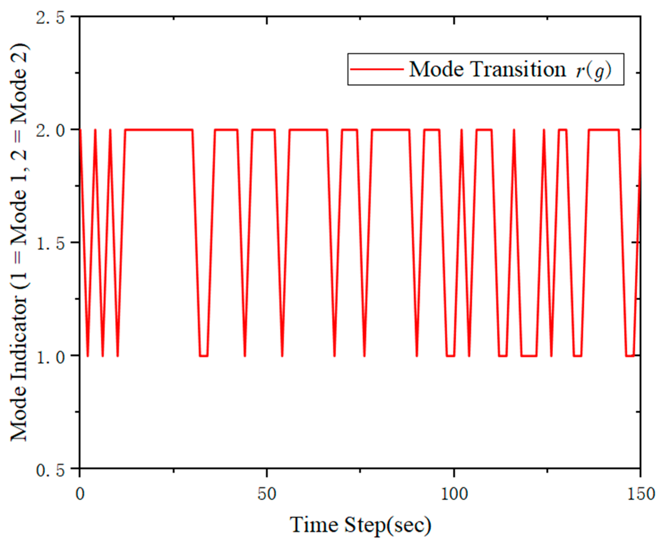
Figure 1 illustrates the discrete mode switching process of the semi-Markov jump system over time. The y-axis represents the system mode index, where ‘1.0’ corresponds to Mode 1 and ‘2.0’ corresponds to Mode 2. This figure provides a visual representation of the mode switching dynamics, showing how the system transitions between different states throughout the simulation.

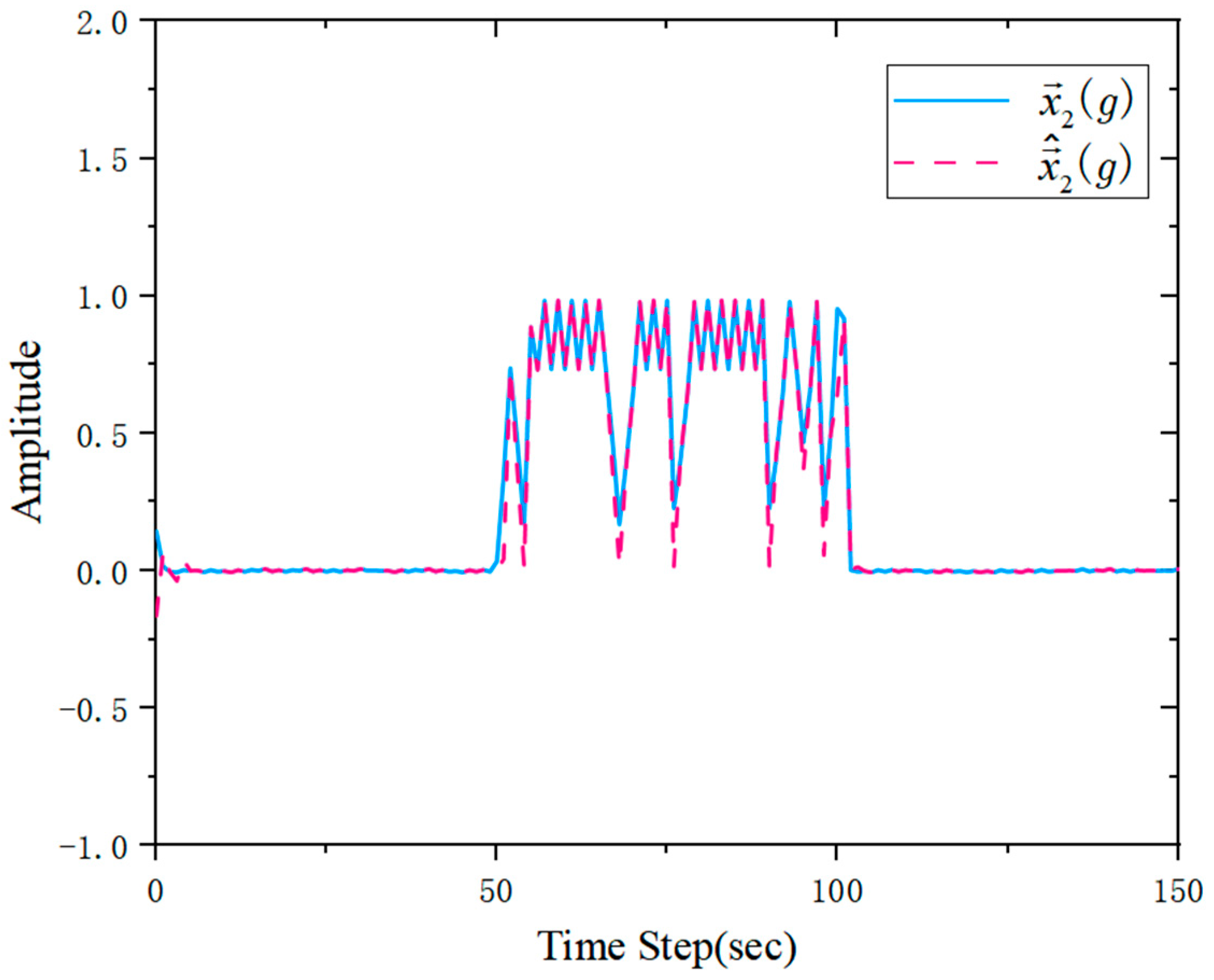
Figure 2 and Figure 3 illustrate the actual and estimated state trajectories ×1 and ×2 under different system modes. The close correspondence between the actual states (solid lines) and their estimates (dashed lines) validates the effectiveness of the proposed observer in accurately tracking system dynamics. Notably, the estimation of sensor faults is not explicitly visualized as a separate plot. Instead, its effects are inherently embedded within the state estimation process. Since sensor faults directly alter the system’s measured outputs, they subsequently affect the estimated state trajectories. This influence manifests as deviations between the actual and estimated states, particularly during fault occurrences.

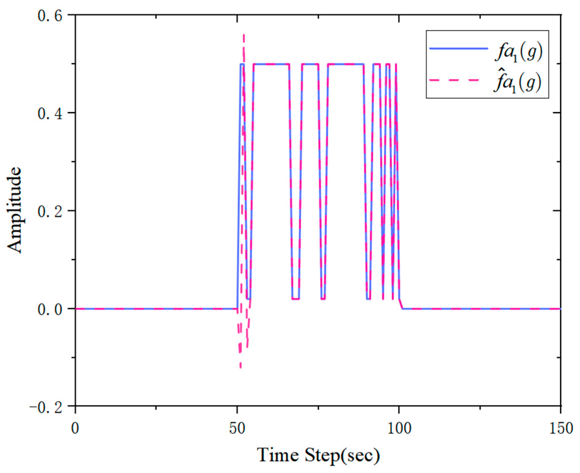
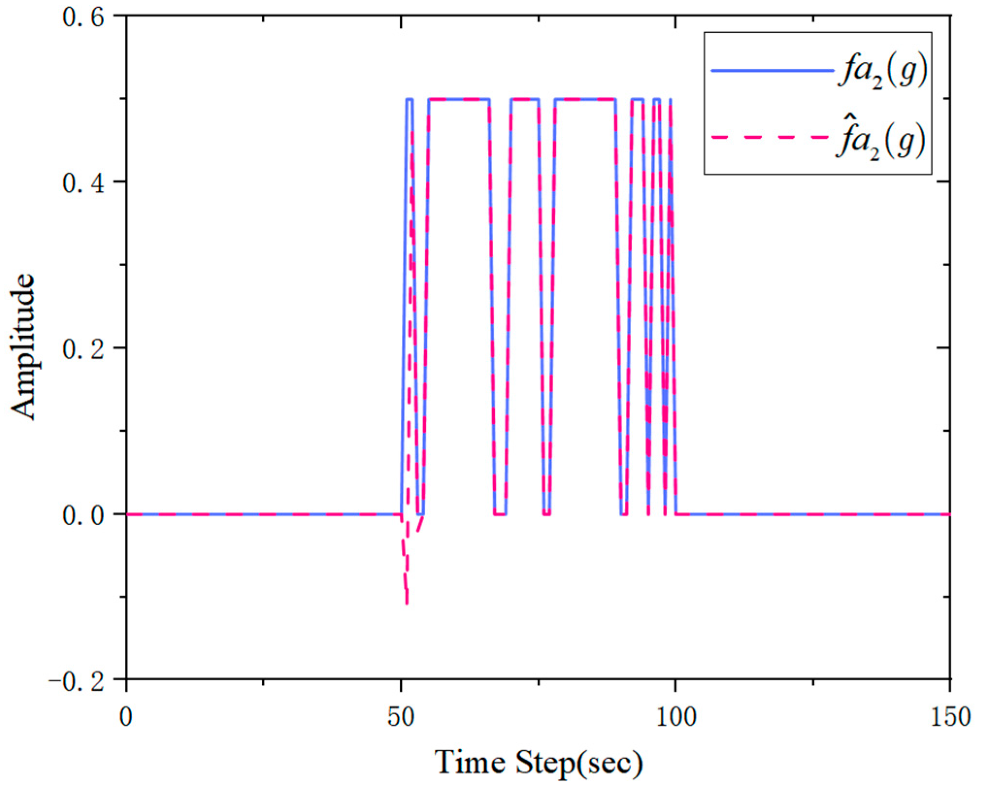
Figure 4 and Figure 5 present the estimation results of actuator faults $f{a}_1(g)$ and $f{a}_2(g)$, respectively. The comparison between the actual fault signals (solid lines) and their estimates (dashed lines) demonstrates the accuracy of the proposed observer. It is noteworthy that transient negative values appear at the initial occurrence of faults. This phenomenon arose due to the observer’s adaptive response, where estimation oscillations were observed before stabilizing. Such behavior was particularly evident in the actuator fault estimation, as the observer dynamically adjusted to minimize estimation errors and improve convergence. These results confirm that the proposed method effectively captured actuator faults while ensuring robust fault estimation performance.

Figure 6 illustrates the estimated output signal $\overrightarrow{z}(g)$, demonstrating the effectiveness of the observer in accurately tracking the system’s measured output under different modes. When faults occur, transient deviations are observed due to the system’s response to faults. These fluctuations gradually diminish as the observer adjusts to the new conditions, ensuring accurate and stable output estimation. The results demonstrate that the proposed observer can accurately estimate the system’s output even in the presence of faults, providing reliable fault estimation for subsequent fault-tolerant control.

Based on these results, it can be concluded that the proposed state and fault estimation algorithm is effectively applicable to discrete-time s-MJNNs with time-varying delays and demonstrates accurate fault estimation capabilities for the system.

5. Conclusions

This paper investigated the dissipative fault estimation problem for discrete-time semi-Markov jump neural networks (s-MJNNs) under the influence of actuator and sensor faults, incorporating the implementation of a round-robin protocol (RRP). To accurately estimate the system states and faults, an extended state observer was developed. By employing the RRP, network congestion was effectively mitigated, and active sensors were dynamically scheduled at each sampling instance, optimizing system resource utilization. A series of sufficient conditions were derived, and the estimator gain parameters were designed to ensure that the error system achieves mean square exponential stability (MSES) and strict $({\chi }_1,{\chi }_2,{\chi }_3)-\varpi$ dissipative performance. The results of the numerical simulations further validate the effectiveness and feasibility of the proposed method.

Despite its demonstrated theoretical and simulation-based advantages, there remain several open questions for further exploration. For instance, building upon the proposed fault estimation framework to achieve fault-tolerant control that reduces conservatism and enhances robustness remains a critical area of future research. Additionally, extending this approach to more complex network systems and integrating advanced communication protocols with real-time control strategies will provide new opportunities to enhance its practical engineering applicability.

References

1. Wei, Y.; Qiu, J.; Karimi, H.; Ji, W. A novel memory filtering design for semi-Markovian jump time-delay systems. IEEE Trans. Syst. Man Cybern. Syst. 2018, 48, 2229–2241. [Google Scholar] [CrossRef]
2. Mollajan, A.; Iranmanesh, H.; Khezri, A.; Abazari, A. Effect of applying independence axiom of Axiomatic Design theory on performance of an Integrated Manufacturing Information System: A computer simulation modeling approach. Simulation 2022, 98, 535–561. [Google Scholar] [CrossRef]
3. Qiu, J.; Wei, Y.; Wu, L. A novel approach to reliable control of piecewise affine systems with actuator faults. IEEE Trans. Circuits Syst. II Express Briefs 2017, 64, 957–961. [Google Scholar] [CrossRef]
4. Chen, F.; Jiang, R.; Zhang, K.; Jiang, B.; Tao, G. Robust Backstepping Sliding Mode Control and Observer-based Fault Estimation for a Quadrotor UAV. IEEE Trans. Ind. Electron. 2016, 63, 5044–5056. [Google Scholar] [CrossRef]
5. Guo, Y.; Jiang, B.; Zhang, Y. A novel robust attitude control for quadrotor aircraft subject to actuator faults and wind gusts. IEEE/CAA J. Autom. Sin. 2018, 5, 292–300. [Google Scholar] [CrossRef]
6. Rong, L.; Peng, X.; Zhang, B. A reduced-order fault detection filter design for polytopic uncertain continuous-time Markovian jump systems with time-varying delays. Int. J. Control Autom. Syst. 2018, 16, 2021–2032. [Google Scholar] [CrossRef]
7. Zhang, B.; Zheng, W.X.; Xu, S. Filtering of Markovian Jump Delay Systems Based on a New Performance Index. IEEE Trans. Circuits Syst. I Regul. Pap. 2013, 60, 1250–1263. [Google Scholar] [CrossRef]
8. Lin, W.J.; He, Y.; Zhang, C.K.; Wang, Q.G.; Wu, M. Reachable Set Estimation for Discrete-Time Markovian Jump Neural Networks With Generally Incomplete Transition Probabilities. IEEE Trans. Cybern. 2021, 51, 1311–1321. [Google Scholar] [CrossRef]
9. Zhang, Y.; Shi, P.; Agarwal, R.K.; Shi, Y. Event-Based Dissipative Analysis for Discrete Time-Delay Singular Jump Neural Networks. IEEE Trans. Neural Netw. Learn. Syst. 2020, 31, 1232–1241. [Google Scholar] [CrossRef]
10. Naifar, O.; Ben Makhlouf, A.; Hammami, M.A.; Ouali, A. State feedback control law for a class of nonlinear time-varying system under unknown time-varying delay. Nonlinear Dyn. 2015, 82, 349–355. [Google Scholar] [CrossRef]
11. Shen, H.; Wu, Z.G.; Park, J.H. Reliable mixed passive and filtering for semi-Markov jump systems with randomly occurring uncertainties and sensor failures. Int. J. Robust Nonlinear Control 2014, 25, 3231–3251. [Google Scholar] [CrossRef]
12. Hu, J.; Wang, Z.; Gao, H.; Stergioulas, L.K. Extended Kalman filtering with stochastic nonlinearities and multiple missing measurements. Automatica 2012, 48, 2007–2015. [Google Scholar] [CrossRef]
13. Liu, S.; Wang, Z.; Chen, Y.; Wei, G. Protocol-Based Unscented Kalman Filtering in the Presence of Stochastic Uncertainties. IEEE Trans. Autom. Control 2020, 65, 1303–1309. [Google Scholar] [CrossRef]
14. Cheng, J.; Park, J.H.; Wu, Z.G. Observer-Based Asynchronous Control of Nonlinear Systems With Dynamic Event-Based Try-Once-Discard Protocol. IEEE Trans. Cybern. 2022, 52, 12638–12648. [Google Scholar] [CrossRef] [PubMed]
15. Ding, D.; Wang, Z.; Han, Q.-L. Neural-network-based output-feedback control with stochastic communication protocols. Automatica 2019, 106, 221–229. [Google Scholar] [CrossRef]
16. Liu, H.; Wang, Z.; Fei, W.; Li, J. H(infinity) and l(2)-l(infinity) state estimation for delayed memristive neural networks on finite horizon: The Round-Robin protocol. Neural Netw. 2020, 132, 121–130. [Google Scholar] [CrossRef]
17. Zou, L.; Wang, Z.; Gao, H.; Liu, X. State Estimation for Discrete-Time Dynamical Networks With Time-Varying Delays and Stochastic Disturbances Under the Round-Robin Protocol. IEEE Trans. Neural Netw. Learn. Syst. 2017, 28, 1139–1151. [Google Scholar] [CrossRef]
18. Sun, L.; Su, L.; Wang, J. Non-fragile dissipative state estimation for semi-Markov jump inertial neural networks with reaction-diffusion. Appl. Math. Comput. 2021, 411, 126404. [Google Scholar] [CrossRef]
19. Xu, Y.; Wu, Z.-G.; Pan, Y.-J. Event-Based Dissipative Filtering of Markovian Jump Neural Networks Subject to Incomplete Measurements and Stochastic Cyber-Attacks. IEEE Trans. Cybern. 2021, 51, 1370–1379. [Google Scholar] [CrossRef]
20. Liu, Y.; Fang, Z.; Park, J.H.; Fang, F. Quantized Event-Triggered Synchronization of Discrete-Time Chaotic Neural Networks With Stochastic Deception Attack. IEEE Trans. Syst. Man Cybern. Syst. 2023, 53, 4511–4521. [Google Scholar] [CrossRef]
21. Cai, T.; Cheng, P.; Yao, F.; Hua, M. Robust exponential stability of discrete-time uncertain impulsive stochastic neural networks with delayed impulses. Neural Netw. 2023, 160, 227–237. [Google Scholar] [CrossRef] [PubMed]
22. Shen, H.; Zhu, Y.; Zhang, L.; Park, J.H. Extended Dissipative State Estimation for Markov Jump Neural Networks With Unreliable Links. IEEE Trans. Neural Netw. Learn. Syst. 2017, 28, 346–358. [Google Scholar] [CrossRef]
23. Sakthivel, R.; Kwon, O.M.; Choi, S.G.; Sakthivel, R. Observer-based state estimation for discrete-time semi-Markovian jump neural networks with round-robin protocol against cyber attacks. Neural Netw. 2023, 165, 611–624. [Google Scholar] [CrossRef]
24. Li, Q.; Zhu, Q.; Zhong, S.; Zhong, F. Extended dissipative state estimation for uncertain discrete-time Markov jump neural networks with mixed time delays. ISA Trans. 2017, 66, 200–208. [Google Scholar] [CrossRef] [PubMed]
25. Zhu, X.; Xia, Y. H∞ descriptor fault detection filter design for T–S fuzzy discrete-time systems. J. Frankl. Inst. 2014, 351, 5358–5375. [Google Scholar] [CrossRef]
26. Zhu, X.; Xia, Y.; Fu, M. Fault estimation and active fault-tolerant control for discrete-time systems in finite-frequency domain. ISA Trans. 2020, 104, 184–191. [Google Scholar] [CrossRef] [PubMed]
27. Yang, H.; Yin, S. Reduced-Order Sliding-Mode-Observer-Based Fault Estimation for Markov Jump Systems. IEEE Trans. Autom. Control 2019, 64, 4733–4740. [Google Scholar] [CrossRef]
28. Zhu, X.; Li, W.; Xia, Y. Finite-time fault estimate and fault-tolerant control for discrete-time Markov jump systems with actuator and sensor faults. Int. J. Robust Nonlinear Control 2023, 33, 6233–6249. [Google Scholar] [CrossRef]
29. Liu, X.; Gao, Z. Integrated fault estimation and fault-tolerant control for stochastic systems with Brownian motions. Int. J. Robust Nonlinear Control 2017, 28, 1915–1941. [Google Scholar] [CrossRef]
30. Han, J.; Zhang, H.; Wang, Y.; Zhang, K. Fault Estimation and Fault-Tolerant Control for Switched Fuzzy Stochastic Systems. IEEE Trans. Fuzzy Syst. 2018, 26, 2993–3003. [Google Scholar] [CrossRef]
31. Li, X.; She, K.; Shi, K.; Cheng, J.; Yu, Y.; Peng, Z. On event-triggered guaranteed cost control for discrete-time semi-Markovian neural networks having communication delays and dual-terminal probabilistic faults. Int. J. Robust Nonlinear Control 2022, 32, 8804–8841. [Google Scholar] [CrossRef]
32. Nam, P.T.; Pathirana, P.N.; Trinh, H. Discrete Wirtinger-based inequality and its application. J. Frankl. Inst. 2015, 352, 1893–1905. [Google Scholar] [CrossRef]
33. Adhira, B.; Nagamani, G.; Soundararajan, G. Exponential extended dissipative performance for delayed discrete-time neural networks under memoryless resilient-based observer design. J. Frankl. Inst. 2022, 359, 5750–5777. [Google Scholar] [CrossRef]
Figure 1. System mode switching in the s-MJNNS.
Applsci 15 05213 g001
Figure 2. State curves x 1 ( g ) and its estimation x ^ 1 ( g ) .
Applsci 15 05213 g002
Figure 3. State curves x 2 ( g ) and its estimation x ^ 2 ( g ) .
Applsci 15 05213 g003
Figure 4. Actuator fault f a 1 ( g ) and its estimation f ^ a 1 ( g ) .
Applsci 15 05213 g004
Figure 5. Actuator fault f a 2 ( g ) and its estimation f ^ a 2 ( g ) .
Applsci 15 05213 g005
Figure 6. Output of z ( g ) and its estimation z ^ ( g ) .
Applsci 15 05213 g006