SPT-AD: Self-Supervised Pyramidal Transformer Network-Based Anomaly Detection of Time Series Vibration Data

Abstract

Bearing fault diagnosis is a key factor in maintaining the stability and performance of mechanical systems, necessitating reliable methods for anomaly detection and prediction. Unlike traditional conservative maintenance approaches, the importance of predictive maintenance where real-time condition monitoring enables proactive preventive measures has been growing steadily. In this study, we propose a deep learning method that effectively discriminates between normal and abnormal bearing conditions, while predicting potential faults in advance. To achieve this, we develop a time series anomaly detection model based on a supervised learning transformer architecture. Our proposed model tackles the data imbalance issue by generating four types of synthetic anomalies from normal vibration data and incorporates a pyramid-structured attention module to reduce computational costs and enhance the handling of long-term dependencies. Experimental results on real bearing vibration datasets demonstrate improved F1-scores over 6%p compared to existing models and demonstrate a significant reduction in computational costs in specific experimental environments. By reliably identifying and predicting bearing faults at an early stage, this research contributes to reducing maintenance costs and improving system stability. Furthermore, it is expected to have wide applicability for state monitoring and anomaly detection in various rotating machinery systems.

1. Introduction

The reliable and sustainable operation of machines plays a crucial role in ensuring productivity, quality, and safety. Rotating components are fundamental to industrial machinery, and their degradation can result in mechanical failures, production downtime, and, in severe cases, catastrophic accidents. Consequently, there is a growing demand for early-stage condition monitoring technologies to detect potential issues and prevent failures before they occur [1,2].

Traditionally, the fault diagnosis of rotating bodies relied primarily on physical inspection and simple sensor-based monitoring methods [3]. However, these approaches are time-consuming and labor-intensive and have many limitations, especially when it comes to detecting defects in early stages [4,5]. These limitations are becoming more pronounced in the context of increasingly complex manufacturing processes and sophisticated facility operations [6]. Recent advances in artificial intelligence have revolutionized many fields. There are various applications such as anomaly detection, image classification, speech recognition, natural language processing, and autonomous driving, and efforts to utilize these technologies in manufacturing industries are increasing [7]. In particular, research on the predictive maintenance of rotating machinery such as motors, Computer Numerical Control Grinding Machines (CNC Grinding Machines), turbines, and generators, which are all bearing equipment common in machinery, is attracting attention as a key technology for realizing smart factories [8]. Predictive maintenance is an approach that utilizes facility data to predict and prevent machine or equipment failures in advance and is more efficient and effective than conventional methods centered on regular inspections [9]. However, as the complexity of facilities increase, maintenance becomes time-consuming and costly, and existing methods are limited to reacting to problems only after they occur [10]. To solve these problems, research on predictive maintenance utilizing AI technology is actively being conducted [11].

Time series data analysis is becoming a core technology for predictive maintenance. The large amount of sensor data collected in the manufacturing processes is unstructured and complex, which makes the early detection of failures and anomalies very difficult [12]. Recently, transformer-based models have shown excellent performance in processing such time series data, providing higher accuracy and faster processing speed than traditional models such as LSTM-AE and AnoGAN [13,14]. This makes them well suited for analyzing large-scale data in real time and detecting anomalous patterns [15].

The ultimate objective of this research is to develop a model that accurately detects anomalous patterns in time series vibration data from bearing systems and predicts potential failures at an early stage. This approach aims to proactively prevent unexpected bearing failures, reduce maintenance costs, and enhance the reliability and efficiency of rotating machinery [16].

In this study, we propose SPT-AD, a transformer-based anomaly detection model designed specifically for bearing fault diagnosis. Furthermore, we introduce an algorithm optimized for the unique characteristics of vibration signals and time series data from rotating machinery. Experimental results demonstrate that SPT-AD outperforms models proposed in recent studies, achieving a 6%p improvement in the F1-score while significantly reducing computational overhead.

This paper is organized as follows. Section 1 describes the background, objectives, and contributions of this research. Section 2 describes bearing signal processing, existing signal processing techniques, research related to predictive maintenance and anomaly detection, and recent research trends. Section 3 describes the structure, learning method, and key differences in the proposed SPT-AD. Section 4 presents the experimental environment, dataset, evaluation method, and experimental results to validate the performance of the proposed model. Finally, Section 5 summarizes the main contributions of this work and discusses limitations and future research directions.

2. Related Work

2.1. Vibration Defects in Rotating Machinery

In mechanical installations, vibration defects typically refer to vibrations that occur when abnormal motion occurs in a machine part or structure. These vibration faults can reveal the reliability, performance, and lifespan of a machine. Therefore, it is important to detect and respond to them early. Vibration faults can be caused by a variety of reasons, including imbalanced parts, misalignment, wear, breakage, interference between machine parts, pressure changes in fluids, poor assembly, and damaged bearings [3,17]. For example, bearing defects cause vibrations with high-frequency components, while gear defects can produce low-frequency vibrations [18]. Identifying these vibration faults typically involves measuring and analyzing the vibration of the machine using sensors such as accelerometers, velocimeters, and displacement meters [2]. This process enables the identification of abnormal vibrations compared to the normal operating state of the machine and determines the causes of the defects. Recent advances in sensor technology and data acquisition devices have created an environment where large-scale vibration data can be analyzed in real time, and if machine learning or deep learning anomaly detection algorithms are utilized, it is possible to monitor facilities in real time and identify defects at an early stage to recognize problems quickly and respond effectively [11].

The analysis of vibration signals plays a key role in fault diagnosis. Signal processing techniques are used to analyze vibration data in the time and frequency domains to extract the characteristics of a fault. The main signal processing techniques include the fast Fourier transform (FFT), short-time Fourier transform (STFT), and wavelet transform (WT) [19,20]. The number of shots determines the signal processing methodology.

The Fourier transform is utilized as a frequency analysis tool in engineering and science [21]. In particular, the FFT is a discrete-time, algorithmic computer implementation of the Fourier transform that is used effectively in a variety of fields. Because the FFT is useful for identifying vibrations, it can be used in statistical anomaly detection to understand the behavior of a machine and find anomalies. To utilize the FFT for anomaly detection, you must first convert the data to the frequency domain using the FFT. The converted frequency spectrum is then analyzed using statistical methods such as mean and standard deviation to identify abnormal frequency components. The anomalous component frequencies are then identified to detect anomalies in the existing data. However, it is difficult to see frequency spectra that change over time because the FFT only analyzes a specific time period and shows the frequency components within a specific bin at once, rather than sequentially. This limits the use of the FFT in mechanical equipment, where it is necessary to see how frequency components change over time. In other words, unlike the Fourier transform, which can only provide information about the frequency components of the entire signal, the STFT can display the differences between the frequency components of the signal at different times [22]. Therefore, the STFT is more effective than the FFT for fault detection in mechanical equipment. In analyzing the time-varying spectrum, it can identify changes in the frequency content of the signal and effectively detect abnormalities that occur in a short period of time. The wavelet transform is a technique that can provide time and frequency information simultaneously, making them well suited for analyzing unstructured and nonlinear vibration signals. There are many variants of wavelet transforms, such as the discrete wavelet transform (DWT), continuous wavelet transform (CWT), and stationary wavelet transform (SWT)  [19]. The DWT can decompose a signal hierarchically to separate high- and low-frequency components, while the CWT is suitable for analyzing changes in a signal over a continuous frequency band. The SWT ensures shift invariance in the signal, allowing it to better capture specific defect features [23].

Traditional vibration signal analysis has predominantly relied on frequency-based methods such as fast Fourier transform (FFT), short-time Fourier transform (STFT), and wavelet transform (WT). However, these approaches often struggle to effectively capture the complex and nonlinear characteristics of real-world machine faults.

To address these limitations, recent studies have highlighted entropy-based techniques as promising alternatives for enhancing fault detection performance by quantifying the irregularity and disorder in signals [24].

• Phase Entropy (PE): This method measures the complexity of signals in phase space, allowing for the detection of subtle variations in nonlinear and chaotic systems [25].
• Multi-scale Entropy (MSE): By analyzing signals across multiple time scales and frequency bands, this approach improves the accuracy of fault detection [26].
• Image Quadrant Entropy (IQE): This technique converts vibration signals into image representations and calculates entropy in different quadrants, enhancing anomaly detection accuracy [27].

These entropy-based approaches provide a robust framework for analyzing complex vibration signals and have demonstrated significant potential in improving fault diagnosis across various engineering applications.

While entropy-based techniques are effective for analyzing signal complexity, they rely on hand-crafted feature extraction, which may limit their generalization ability when applied to complex real-world datasets. In contrast, deep learning-based approaches offer a more powerful alternative by automatically learning hierarchical feature representations from raw vibration signals.

Additionally, various signal processing techniques, such as high-pass and low-pass filtering, the Hilbert transform, and empirical mode decomposition (EMD), are widely used in vibration data analysis. These methods help extract key signal features, facilitating more accurate defect detection and localization.

Traditionally, facility management has consisted primarily of regular preventive inspections and reactive maintenance after a failure has occurred. Preventive maintenance involves inspecting equipment at regular intervals and replacing parts when necessary, an approach that attempts to address problems before they occur. However, this approach can be time-consuming and costly, with the potential for unnecessary maintenance work even when the equipment has not actually failed. Reactive maintenance is an approach for fixing problems after a failure has occurred that can lead to downtime and costly losses. Predictive maintenance is a modern way of predicting and preventing failures in advance based on facility data. Predictive maintenance utilizes IoT sensors and data collection technologies to monitor the health of equipment in real time and assess the likelihood of failure through machine learning and deep learning algorithms [28]. Various algorithms for Remaining Useful Life (RUL) prediction, anomaly detection, and failure diagnosis are being developed to improve equipment utilization and reduce maintenance costs.

2.2. Anomaly Detection

Anomaly detection refers to the process of recognizing deviations in a facility’s operational patterns that significantly differ from normal conditions. This technique is crucial for the early identification and mitigation of potential faults [8]. Conventional methods for anomaly detection primarily rely on statistical analysis and signal processing. These techniques often involve setting thresholds using the mean and standard deviation or identifying anomalies through spectral analysis by examining frequency component variations. In recent years, machine learning and deep learning approaches have increasingly been applied to anomaly detection. Popular machine learning methods include Support Vector Machines (SVMs), Random Forests, and k-means clustering, whereas deep learning models such as Long Short-Term Memory (LSTM) networks, Convolutional Neural Networks (CNNs), and Autoencoders have been utilized for capturing complex anomaly patterns [29]. The strengths of these deep learning techniques are that they can effectively analyze large amounts of complex data and identify subtle anomaly patterns that are difficult to detect using traditional methods.

Detecting anomalies in time series data necessitates understanding temporal dependencies across sequential observations. To achieve this, models like recurrent neural networks (RNNs), Gated Recurrent Units (GRUs), and transformer-based architectures are frequently employed [11]. These techniques are able to learn complex correlations in time series data and detect anomalies more accurately. In this paper, we utilize anomaly detection to identify defects in machinery in the manufacturing industry [30]. The classification of anomaly detection methods varies depending on the characteristics of the dataset. One common approach categorizes these methods based on whether labeled data samples are available.

As illustrated in

Table 1. Types of anomaly detection based on the presence of normal and abnormal data labels.

Category	Normal Data	Abnormal Data
Supervised Anomaly Detection	Yes	Yes
Semi-supervised Anomaly Detection	Yes	No
Unsupervised Anomaly Detection	No Labels Required

, anomaly detection techniques can be divided into three categories based on the utilization of abnormal data and the presence of labels.

Supervised anomaly detection learns using normal and abnormal data with labels, and new data are automatically classified as normal or abnormal by analyzing them with a classifier. It is more accurate than other anomaly detection methods and is used in a wide range of fields, such as in Bayes classifiers and neural networks. However, this method depends on whether there are training data with initial label values. Because outliers are rare, it is generally difficult to obtain a sufficient number of labeled classes. Supervised anomaly detection requires data labeling, making it time-consuming and costly, and mistakes can occur during the labeling process. To compensate for these disadvantages, semi-supervised learning uses a small amount of labeled normal data in what is known as pseudo-labeling. It can save time and costs by not collecting abnormal data, but its accuracy is lower than that of supervised anomaly detection. Unsupervised anomaly detection uses unlabeled data and is widely used in industrial systems due to its ability to process a large amount of data. Principal component analysis and partial least squares are representative examples. However, this method is only effective for data with low correlation, and the data must follow a multivariate Gaussian distribution. Principal component analysis shows the poorest performance among the three anomaly detection methods. The anomaly detection techniques categorized by methodology are summarized in Table 2.

In addition, anomalies, which are data points, bins, or structures that deviate from the normal pattern of the data, can be a sign of system failure, unusual activity, or an event of interest. In time series data, anomalies can be categorized into several types, each of which is defined and detected differently depending on the nature and context of the data. The main types of time series anomalies can be categorized into Global Anomaly, Contextual Anomaly, Shapelet Anomaly, Seasonal Anomaly, and Trend Anomaly [31].

Table 2. Comparison of Time Series Anomaly Detection Methods.

Category	Method	Strengths	Limitations
Statistical	Z-score [32]	Fast, simple, interpretable	Needs normality assumption, sensitive to noise
	ARIMA [33]	Good for trend-based anomalies	Weak for nonlinear data
	Entropy-based [34]	Captures data randomness	High computation cost
Machine Learning	KNN [35]	Works without assumptions	Poor for high-dim data
	SVM [36]	Effective on small data	High cost for large data
	PCA [37]	Reduces complexity	Limited to linear data
Deep Learning	LSTM [38]	Captures long-term dependencies	High training cost
	Autoencoder [39]	Learns normal patterns	Fails if abnormal data are included
	GAN [40]	Learns complex patterns	Unstable training
	Transformer [41]	Strong for sequence data	Needs large dataset

Table 2. Comparison of Time Series Anomaly Detection Methods.

Category	Method	Strengths	Limitations
Statistical	Z-score [32]	Fast, simple, interpretable	Needs normality assumption, sensitive to noise
	ARIMA [33]	Good for trend-based anomalies	Weak for nonlinear data
	Entropy-based [34]	Captures data randomness	High computation cost
Machine Learning	KNN [35]	Works without assumptions	Poor for high-dim data
	SVM [36]	Effective on small data	High cost for large data
	PCA [37]	Reduces complexity	Limited to linear data
Deep Learning	LSTM [38]	Captures long-term dependencies	High training cost
	Autoencoder [39]	Learns normal patterns	Fails if abnormal data are included
	GAN [40]	Learns complex patterns	Unstable training
	Transformer [41]	Strong for sequence data	Needs large dataset

2.3. Transformer

The transformer model was first proposed in natural language processing (NLP) but has recently been widely used in time series data analysis. Transformers use a self-attention mechanism to learn the correlations between each element of the input data and can effectively handle long-term dependencies. Compared to RNNs and LSTMs, this model has the advantage of parallel processing, which make it suitable for large-scale data analysis and time series data analysis, which require real-time processing. In recent research, various models based on transformers have been proposed. For example, models such as the Time Transformer, Informer, and Autoformer were designed to improve the efficiency and accuracy of time series data analysis [42]. These models have been applied to various tasks such as condition monitoring, anomaly detection, and the predictive maintenance of manufacturing facilities and have shown better performance than traditional models.

The main challenge of transformer-based models is to efficiently address large-scale data processing and high computational cost. For this purpose, lightweight model structures, efficient attachment mechanisms, and data augmentation techniques are being researched [43]. In this study, we designed a transformer-based model suitable for time series anomaly detection in manufacturing environments to overcome the limitations of existing techniques.

2.4. Attention Mechanism

The attention mechanism used in transformer-based models is a key technology in modern deep learning that focuses attention on the important elements in the data. It consists of three components—Query, Key, and Value—and learns how each element in the input data relates to all the others to emphasize the most relevant information [6].

In the transformer model, attention is not limited to a single layer but uses multi-head attention to learn different patterns and relationships. Multi-head attention runs multiple independent attention mechanisms in parallel and then combines the results to maximize information representation. This approach helps the model learn complex correlations in the input data and capture multidimensional patterns in the data [44]. Transformer models originated in natural language processing (NLP) but have recently been widely used in time series data analysis. Modern models, such as the Time Transformer, Informer, and Autoformer, are designed to reflect the characteristics of time series data and excel at anomaly detection and predictive maintenance in manufacturing environments. These models have efficiently improved self-attention to reduce computational cost and improve the ability to handle large-scale data.

The self-attention mechanism is a particularly powerful tool in time series data analysis. By learning how each point in time in the input data interacts with all other points in time, it captures the complex temporal correlations in time series data [43]. The self-attention mechanism thus overcomes the limitations of traditional recurrent neural network (RNN) or LSTM-based models and can be computed in parallel, greatly improving computational efficiency. One of the key challenges of the attention mechanism is its high computational complexity. As the computational cost increases rapidly when processing long-sequence data, efficient mechanism designs such as Log-sparse Attention, Sparse Attention, and Autocorrelation Attention have been studied. Sparse Attention, which is a recent representative design, increases computational efficiency by selectively learning the interactions between important elements without computing the relationships between all elements in the input data. These techniques are particularly useful in tasks that deal with large amounts of data, such as manufacturing environments [45].

3. SPT-AD: Self-Supervised Pyramidal Transformer Network-Based Anomaly Detection

3.1. Model Framework

Self-Supervised Pyramidal Transformer Network-Based Anomaly Detection (SPT-AD) is a transformer-based algorithm that performs time series anomaly detection by generating anomaly data through self-supervised learning. An algorithm called AnomalyBERT was proposed based on the motif of BERT, which uses only the encoder structure of the transformer [46]. In this paper, we propose a new architecture SPT-AD based on the AnomalyBERT architecture, which replaces the core component of the multi-head self attention (MSA) with the Pyramidal Attention Module (PAM) of Pyraformer and adds a Coarse-Scale Construction Module (CSCM) to improve the anomaly detection performance and computational efficiency of time series data [47]. The proposed model overcomes data imbalance while maintaining synthesis outliers through a data degradation method and effectively learns temporal and inter-variable correlations utilizing multi-resolution representation through the Pyramidal Attention Module. This section describes the proposed model structure and algorithms in detail. The overall structure of the model is shown in Figure 1.

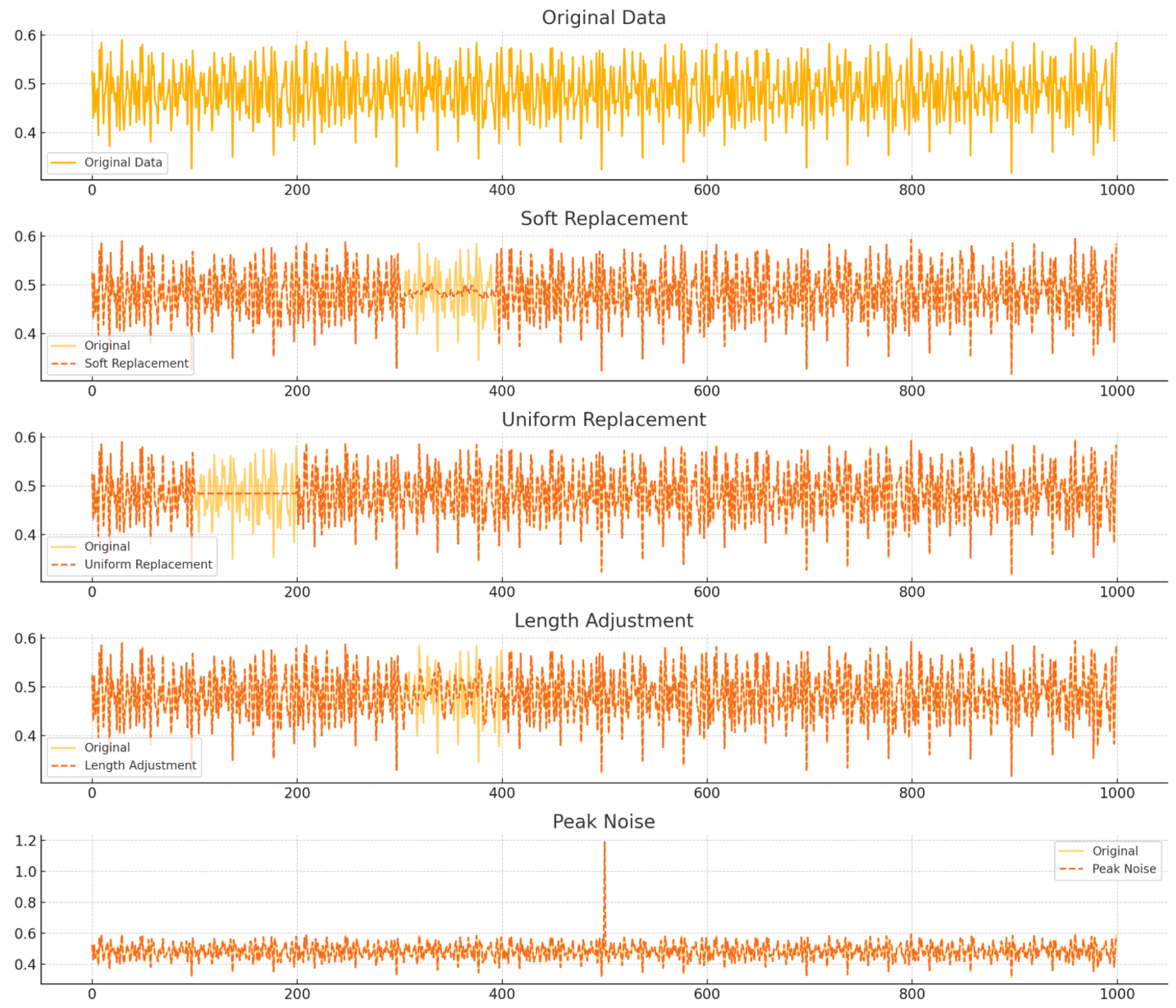
SPT-AD uses four synthesis outlier methods proposed in AnomalyBERT to generate outlier data and learn outlier patterns by comparing the original data with the degraded data when training the model. The four types of synthesis outliers used are as follows. They can also be seen in Figure 2.

Our approach to data degradation methods include the following elements:

• Soft Replacement: Soft replacement is a method of replacing missing values or outliers in time series data utilizing a specific combination of weights for values outside a window that contains data around those values.
• Uniform Replacement: Uniform replacement is a method of replacing missing values or outliers with a single, fixed, constant value. This value can be chosen as a logical default for the data, or it can be the mean, median, or a specific reference value.
• Length Adjustment: Length adjustment is a technique for adjusting the length of time series data, stretching or shrinking the data to make them the right length when they do not meet your analysis needs.
• Peak Noise: Peak noise is a technique for inserting unusually high peak values at specific points in time series data; it is useful for testing the noisy nature of data or observing the response of a system.

In the Linear Embedding Layer Map, each point in the time series data is embedded into a high-dimensional space to create an initial embedding vector as input for the transformer model. Input data are denoted as $X=[x_1,x_2,\cdots ,x_n]\in {\mathbb{R}}^{N\times D_{\mathrm{input}}}$, where N is the length of the time series, and D is the dimension of each data point. Output data are denoted as $X_{\mathrm{embed}}=[e_1,e_2,\cdots ,e_N]\in {\mathbb{R}}^{N\times D_{\mathrm{embed}}}$.

The Coarse-Scale Construction Module (CSCM) is a module that converts time series data into multi-resolution layers, compressing the information in the time series at each resolution and passing it on to higher layers. Each resolution is generated by 1D convolution using a kernel and stride of C-Scale. If the input time series data are $X_{\mathrm{embed}}\in {\mathbb{R}}^{N\times D_{\mathrm{embed}}}$, the CSCM reduces the data length to N/C at each layer. The final output consists of a feature vector $X_{\mathrm{CSCM}}$ of multi-resolution layers.

$$X_{\mathrm{CSCM}}=[X_1,X_2,\cdots ,X_s]\in {\mathbb{R}}^{(N+{\displaystyle \frac{N}{C}}+\cdots +{\displaystyle \frac{N}{C^{S-1}}})\times D_{\mathrm{hidden}}}$$

(1)

(S: number of resolution layers, C: convolution stride).

The transformer body is composed of multiple layers of Pyramidal Attention Module (PAM) and Feed Forward (Multilayer Perceptron, MLP) blocks. The Pyramidal Attention Module is used to learn temporal patterns and interactions between variables in time series data. The final output of the transformer body is a latent feature vector, $H\in {\mathbb{R}}^{N\times D_{\mathrm{hidden}}}$. where A is the length of the time series window. N is the length of the time series window (number of data points), and $D_{\mathrm{hidden}}$ is the feature dimensionality generated by the transformer body.

The Pyramidal Attention Module is a multi-resolution-based attention mechanism proposed in Pyraformer, which is used as an alternative to multi-head self attention (MSA).

Our approach’s attention module includes the following elements:

• Inter-scale Attention: Soft replacement replaces missing values or outliers in time series data utilizing a specific combination of weights for values outside a window containing data around those values.

  $$H_{\mathrm{inter}}^{\left(s\right)}=\mathrm{Softmax}\left({\displaystyle \frac{Q^{\left(s\right)}{K}^{{(s+1)}^T}}{\sqrt{d}}}\right)V^{(s+1)}$$

  (2)
• Intra-scale Attention: This learns the interactions between neighboring nodes within each resolution, exchanging information between neighboring nodes in the same resolution succession.

  $$H_{\mathrm{intra}}^{\left(s\right)}=\mathrm{Softmax}\left({\displaystyle \frac{Q^{\left(s\right)}{K}^{{\left(s\right)}^T}}{\sqrt{d}}}\right)V^{\left(s\right)}$$

  (3)

The Pyramidal Attention Module synthesizes multi-resolution information to generate a potential feature vector, $H_{\mathrm{PAM}}\in {\mathbb{R}}^{N\times D_{\mathrm{hidden}}}$. Combining inter-scale and intra-scale attention reduces the computational complexity of the transformer from $O\left(L^2\right)$ to $O\left(L\right)$ and enables efficient learning while maintaining temporal dependencies even on long time series data.

The Prediction Block is the final step in APT-AD, which calculates an outlier score (0 to 1) for each time series point from the output of the transformer body. The model is trained by comparing it to the outlier bins generated by applying synthesis outliers. The potential feature vector $H=[h_1,h_2,\cdots ,h_N]$, which is the output of the transformer body, is input into the Prediction Block, which outputs the anomaly score $A=[a_1,a_2,\cdots ,a_N]$. Each feature vector $h_i$ is transformed into a single value $a_i$ through a linear transformation and normalization function.

$$H=[h_1,h_2,\cdots ,h_N]\in {\mathbb{R}}^{N\times D_{\mathrm{hidden}}}$$

(4)

$$z_i=W{h}_i+b$$

(5)

$$a_i=\sigma \left(z_i\right)$$

(6)

$$A=[a_1,a_2,\cdots ,a_N]\in {\mathbb{R}}^{N\times 1}$$

(7)

Here, W is the trainable weight matrix, b is the bias value, $z_i$ is the anomaly score before normalization, and $\sigma$ is the normalization function (Sigmoid), and the final output A is expressed as the anomaly score for each time series point, where the closer the value of $a_i$ is to 1, the more likely the data point is to be an anomaly. As a result, the overall behavior of the Prediction Block can be expressed as follows:

$$A=\sigma (H{W}^T+b)$$

(8)

The Prediction Block is trained with Binary Cross Entropy Loss by comparing the predicted outlier scores with the outlier data labels generated by the synthesis outliers. The loss function is defined as follows:

$$L=-{\displaystyle \frac{1}{N}}\sum _{i=1}^N\left(y_{i}log\left(a_i\right)+(1-y_i)log(1-a_i)\right)$$

(9)

($y_i\in \{0,1\}$: degraded data labels: 0 (normal), 1 (anomaly); $a_i\in [0,1]$: anomaly scores output from the Prediction Block).

3.2. SPT-AD Algorithm

As shown in Algorithm 1, the given input data $X=[x_1,x_2,\cdots ,x_N]\in {\mathbb{R}}^{N\times D_{\mathrm{input}}}$ consist of time series data, where N data points are arranged along the time axis, and each data point is represented as a $D_{\mathrm{input}}$-dimensional vector. These input data are projected into a high-dimensional latent space through a linear transformation defined as

$$X_{\mathrm{embed}}=X{W}_{\mathrm{embed}}+b_{\mathrm{embed}}$$

(10)

where $W_{\mathrm{embed}}$ is the weight matrix used to project the input data into the latent space, and $b_{\mathrm{embed}}$ is the bias vector added to the projected vector. This allows the input data to gain richer representation in the high-dimensional space. Then, the initial latent representation is set as

$$X^{\left(1\right)}=X_{\mathrm{embed}}^{\prime }$$

(11)

where $X_{\mathrm{embed}}^{\prime }$ denotes the normalized or further transformed $X_{\mathrm{embed}}$.

For scales $s=1,\cdots ,S$, multi-scale convolution is performed iteratively. In this process, the convolution operation is applied using

$$X^{\left(s\right)}={\mathrm{Conv}}_C\left(X^{(s-1)}\right)$$

(12)

where kernel size and stride are utilized. The features extracted at different scales are then combined as

$$X_{\mathrm{CSCM}}=[X^{\left(1\right)},X^{\left(2\right)},\cdots ,X^{\left(S\right)}]$$

(13)

The dimensionality of this combined scale feature is defined as

$$X_{\mathrm{CSCM}}\in {\mathbb{R}}^{L\times D_{\mathrm{embed}}},\mathrm{where}L=N+\sum _{s=2}^S{\displaystyle \frac{N}{C^{s-1}}}$$

(14)

where L represents the extended length of the time series data through multi-scale convolution.

For each attention layer $l=1,\cdots ,L_{\mathrm{attn}}$, inter-scale attention and intra-scale attention are computed. The inter-scale attention is defined as

$$H_{\mathrm{inter}}^{\left(s\right)}=\mathrm{Softmax}\left({\displaystyle \frac{Q^{\left(s\right)}{K}^{{(s+1)}^T}}{\sqrt{d}}}\right)V^{(s+1)}$$

(15)

and the intra-scale attention is defined as

$$H_{\mathrm{intra}}^{\left(s\right)}=\mathrm{Softmax}\left({\displaystyle \frac{Q^{\left(s\right)}{K}^{{\left(s\right)}^T}}{\sqrt{d}}}\right)V^{\left(s\right)}$$

(16)

All the attention results extracted from different scales are combined to form the multi-resolution feature representation

$$H_{\mathrm{PAM}}=[H^{\left(1\right)},H^{\left(2\right)},\cdots ,H^{\left(S\right)}]$$

(17)

Subsequently, for each time series point $i=1,\cdots ,N$, a linear transformation is computed as

$$z_i=W_{\mathrm{pred}}{h}_i+b_{\mathrm{pred}}$$

(18)

This value is transformed through sigmoid normalization as

$$a_i=\sigma \left(z_i\right),\sigma \left(z_i\right)={\displaystyle \frac{1}{1+e^{-z_i}}}$$

(19)

Finally, the anomaly scores are returned as

$$A=[a_1,a_2,\cdots ,a_N]$$

(20)

where each $a_i$ represents the anomaly score for the corresponding time step.

Algorithm 1 SPT-AD Algorithm

Require: Input time series data $X=[x_1,x_2,\cdots ,x_N]\in {\mathbb{R}}^{N\times D_{\mathrm{input}}}$ 1: Step 1: Project Input to Latent Space 2: $X_{\mathrm{embed}}=X{W}_{\mathrm{embed}}+b_{\mathrm{embed}}$  ▷Linear transformation using weights $W_{\mathrm{embed}}$ and bias $b_{\mathrm{embed}}$ 3: $X^{\left(1\right)}=X_{\mathrm{embed}}^{\prime }$   ▷Normalization or further transformation of $X_{\mathrm{embed}}$ 4: Step 2: Apply Multi-Scale Convolution 5: for $s=1$ to S do 6:     $X^{\left(s\right)}={\mathrm{Conv}}_C\left(X^{(s-1)}\right)$   ▷Apply convolution at scale s 7: end for 8: Combine features: $X_{\mathrm{CSCM}}=[X^{\left(1\right)},X^{\left(2\right)},\cdots ,X^{\left(S\right)}]$ 9: Compute dimensionality: $X_{\mathrm{CSCM}}\in {\mathbb{R}}^{L\times D_{\mathrm{embed}}}$, where $L=N+{\sum }_{s=2}^S{\displaystyle \frac{N}{C^{s-1}}}$ 10: Step 3: Compute Attention Scores 11: for $l=1$ to $L_{\mathrm{attn}}$ do 12:     for $s=1$ to S do 13:         Compute inter-scale attention: $H_{\mathrm{inter}}^{\left(s\right)}=\mathrm{Softmax}\left({\displaystyle \frac{Q^{\left(s\right)}{K}^{(s+1)T}}{\sqrt{d}}}\right)V^{(s+1)}$ 14:         Compute intra-scale attention: $H_{\mathrm{intra}}^{\left(s\right)}=\mathrm{Softmax}\left({\displaystyle \frac{Q^{\left(s\right)}{K}^{\left(s\right)T}}{\sqrt{d}}}\right)V^{\left(s\right)}$ 15:     end for 16: end for 17: Combine attention results: $H_{\mathrm{PAM}}=[H^{\left(1\right)},H^{\left(2\right)},\cdots ,H^{\left(S\right)}]$ 18: Step 4: Compute Anomaly Scores 19: for each time series point $i=1,\cdots ,N$ do 20:     $z_i=W_{\mathrm{pred}}{h}_i+b_{\mathrm{pred}}$   ▷Linear transformation 21:     $a_i=\sigma \left(z_i\right)={\displaystyle \frac{1}{1+e^{-z_i}}}$   ▷Sigmoid normalization 22: end for 23: Output: $A=[a_1,a_2,\cdots ,a_N]$   ▷Anomaly scores for each time step

4. Experiment and Results

4.1. Experimental Environments

In this study, we conducted experiments on time series anomaly detection using the proposed SPT-AD model. The experiments were conducted using Tesla L4 GPUs from Google Colab. The L4 GPU is designed based on the latest Lovelace Architecture, and its main specifications are shown in

Table 3. Computing resource spec.

	CUDA Core	Tensor Core	GPU Memory	FP32	FP16
Computing resource spec.	7424	192	24 GB GDDR6	29.2 TFLOPs	145 TFLOPs

.

The development environment used Python 3.8.10, CUDA 11.2, cuDNN 8, PyTorch 1.12, and Numpy 1.21 built on Ubuntu 18.04 OS via the Google Colab platform (

Table 4. Development environment.

	OS	CUDA	cuDNN	Python	PyTorch
Development environment	Unbuntu 18.04	v11.2	v8	v3.8.10	v1.12

).

4.2. Data Preprocessing

We used the Machinery Fault Simulator (MFS) dataset to conduct our experiments. The MFS testbed was built to collect a sufficient amount of failure data (i) to characterize different failure types of rotating machines, which are used as major equipment in most industrial sites, and (ii) to classify their normal and faulty states. The data generated, which are similar to the fault types of real rotating equipment, enabled experimentation on various tests such as machine learning- and deep learning-based fault prediction and fault classification. Figure 3 shows the rotating equipment MFS testbed used for experimental data collection.

The experiment was performed using an MFS testbed built to generate failure data for rotating equipment, collecting vibration data for the steady state and three bearing failure types (normal, cage failure, lack of lubrication, and oxidation). Waveforms of the bearing data used in the test are shown in Figure 4.

The data system used for bearing defect vibration data acquisition was designed for high-speed data acquisition. It consists of an IEPE acceleration sensor, a Signal Conditioner (SC), a Data Acquisition Module (DAQ), and an Edge Computing Module. The analog signal generated by the sensor is preprocessed in the Signal Conditioner, and the Data Acquisition Module samples the signal up to 20,000 Hz and stores it in the IoT or cloud. During this process, the collected data undergo normalization, signal filtering, and noise reduction. Figure 5 shows the data acquisition system. Figure 6 and Figure 7 show an image of the IEPE acceleration sensor used and mounted on the MFS testbed. The monitoring locations and time points were pre-defined according to the design of the MFS testbed.

The vibration data used in the experiment were sampled at 1000 Hz for each data type and collected for 5 min. At this time, the rotating motor was running at 1500 RPM. The data types were categorized into five types of bearing defects: normal bearing, high-speed damaged bearing, cage defect, lack of lubricant, and oxidized condition.

For the MFS dataset, data were collected from each of the three axes of the sensor (X, Y, Z) at a sampling rate of 1000 Hz. Among the five types of bearing faults mentioned above, we used [1,800,000, 3] data samples collected from three types of faulty bearings (Fault1, Fault2, Fault3) and three types of normal bearings (Normal1, Normal2, Normal3) for 5 min each and a total of 30 min, excluding the two types where the variability of the data was too large to reduce the generalization performance of the model. The data in each file were split using a sliding window method with a window size of 512 and slide spacing of 256 (50% overlap), resulting in a sequence of N × 512. All data samples were then normalized using Min-Max Scaling in the range of 0 to 1. The maximum and minimum values of the data samples were calculated from the previous data (noise was removed using the DAQ system and replaced with the average of the neighboring data) and labeled as 0 for normal data and 1 for abnormal data for each sequence. The preprocessed data were stored in Numpy format, the normal sequence data and labels were used as training data, and the normal and abnormal sequence data and labels were used as test data. JSON files were created and processed for each sensor’s channel information and normal and abnormal class information. Hyperparameter values were chosen experimentally to optimize model performance. The input data followed a structured format with a batch size of 32, a window size of 512, a patch size of 4, and three input features. A sliding window approach with a step size of 256 was used to capture temporal dependencies. The learning rate was set to 0.0001, and the training process was conducted over a maximum of 10,000 iterations. The model consisted of a transformer architecture with six layers, incorporating a dropout rate of 0.1 to prevent overfitting. The resolution of the data was represented by r_size values of 256, 128, and 64 across three hierarchical levels (r_level). For optimization, Binary Cross Entropy (BCE) was employed as the loss function. The hyperparameters can be found in

Table 5. Hyperparameter settings.

Parameter	Value
learning rate	0.0001
summary_steps	500
max_steps	10,000
batch_size	32
window_size	512
n_features	3
patch_size	4
d_embed	512
n_layer	6
dropout	0.1
window_sliding	256
r_level	3
r_size	256, 128, 64
loss function	BCE

.

4.3. Performance Metrics

To evaluate the performance of the proposed model, SPT-AD, five evaluation metrics, namely the accuracy, precision, recall, F1-score, and AUROC curve, were used as performance indicators in this study.

Accuracy is a metric that measures the percentage of all predictions made by a model that match the true value. This gives you an idea of how accurately the model is at predicting.

$$\mathrm{Accuracy}={\displaystyle \frac{\mathrm{TP}+\mathrm{TN}}{\mathrm{TP}+\mathrm{FN}+\mathrm{FP}+\mathrm{TN}}}$$

(21)

T and P are true and false, respectively, for whether the model predicted correctly, and P and N are positive and negative, respectively, for whether the value predicted by the model was positive or negative. This is a metric that evaluates how many of the total predictions are correct, like a formula, but it can overestimate performance in data-imbalanced environments where only certain classes of data are abundant.

Precision is a measure of the percentage of true positives (TP) in the actual data that the model predicts are actually positive. Precision indicates how accurate the results predicted to be positive are.

$$\mathrm{Precision}={\displaystyle \frac{\mathrm{TP}}{\mathrm{TP}+\mathrm{FP}}}$$

(22)

Recall is a measure of the percentage of positives in the actual data that the model predicts are positive. Recall indicates how well the model predicts positives without missing any.

$$\mathrm{Recall}={\displaystyle \frac{\mathrm{TP}}{\mathrm{TP}+\mathrm{FN}}}$$

(23)

The F1-score is a metric used to evaluate the performance of a binary classification model, measuring balanced performance through the harmonic mean of precision and recall. Precision refers to the proportion of positive predictions that are actually positive, while recall refers to the proportion of true positives that the model correctly predicts. The F1-score has a value between 0 and 1, with higher values indicating a model that balances precision and recall.

$$\mathrm{F}1-\mathrm{score}=2\times {\displaystyle \frac{\mathrm{Precision}\times \mathrm{Recall}}{\mathrm{Precision}+\mathrm{Recall}}}$$

(24)

F1 is the product of precision and recall. Unlike precision, it is susceptible to smaller values, allowing models to be evaluated effectively in data-imbalanced environments.

The curve that evaluates the performance of a model as the threshold between 0 and 1, which determines whether a prediction is true or false, is called the ROC curve. The area under the ROC is called the AUC. The AUC value is a value between 0 and 1, and the closer it is to 1, the better the performance.

$$AUROC={\int }_0^1\mathrm{True}\mathrm{Positive}\mathrm{Rate}\left(\mathrm{TPR}\right)·d\left(\mathrm{False}\mathrm{Positive}\mathrm{Rate}\left(\mathrm{FPR}\right)\right)$$

(25)

These performance metrics were used to quantify and compare the time series anomaly detection performance of SPT-AD models. They provide a comprehensive view of the model’s performance by evaluating the model’s accuracy, precision, recall and F1-score.

4.4. Results

Figure 8 illustrates the application of synthetic outlier generation methods to the original data. We utilized four types of synthetic outliers: soft replacement, uniform replacement, length adjustment, and peak noise. Each method was designed to allow the model to indirectly learn the characteristics of abnormal data without requiring labeled anomaly data.

• Soft Replacement: This method introduces subtle changes by replacing portions of the original data with smoothed values. It reflects gradual anomalies that appear over time, enabling the model to detect progressive deviations.
• Uniform Replacement: This method replaces parts of the original data with random values generated from a uniform distribution. It simulates abrupt and unpredictable changes, mirroring sudden failures or external disturbances in sensor data.
• Length Adjustment: Segments of the time series data are modified to reflect changes in periodicity or amplitude. This mimics real-world phenomena such as equipment wear or performance degradation.
• Peak Noise: Sharp, isolated spikes are injected into the data to represent transient anomalies caused by mechanical impacts or electrical disturbances. This type of noise is designed to handle highly localized yet critical anomaly scenarios effectively.

By generating synthetic outliers from normal data, the proposed SPT-AD model reduces reliance on labeled anomaly data and strengthens its generalization ability for diverse real-world scenarios. These techniques also minimize preprocessing requirements for large-scale sensor data, lowering the barriers to industrial deployment.

Figure 9 shows the comparison of performance metrics (accuracy, precision, recall, and F1-score) between the LSTM Autoencoder, AnomalyBERT, and proposed SPT-AD model. Each metric was used as the main criterion to evaluate the anomaly detection performance of the model. This demonstrates that the design utilizing data degradation techniques and multi-resolution processing was effective, showing that the SPT-AD model provides higher accuracy and balanced precision and recall in anomaly detection compared to the existing models.

In this study, we conducted an experiment to assess the performance of SPT-AD, a transformer-based time series anomaly detection model using self-supervised learning. We evaluated the performance of three models—LSTM AutoEncoder, MSCRED, USAD AnomalyBERT—that are widely used in unbalanced data problems and the proposed model, SPT-AD and used Accuracy, precision, recall, and F1-score as evaluation metrics. The results can be seen in

Table 6. Comparison with other models.

Model	Accuracy	Precision	Recall	F1-Score
LSTM Autoencoder	0.621	0.645	0.585	0.614
MSCRED	0.590	0.612	0.568	0.589
USAD	0.709	0.763	0.655	0.705
AnomalyBERT	0.768	0.856	0.652	0.740
SPT-AD	0.814	0.882	0.746	0.809

. Since it is an anomaly detection problem utilizing only normal data, the performance metrics tended to be low, and the recall was somewhat low, but overall, the SPT-AD model proposed in this paper performed well.

Table 7. Comparison of computations.

Model	Complexity	FLOPs
AnomalyBERT (MSA)	$O\left(N^{2}d\right)$	50.7 GFLOPs
SPT-AD (PAM)	$O(NlogNd)$	21.83 GFLOPs

shows a comparison of the computational effort of AnomalyBERT and SPT-AD. Computation was mainly calculated based on the Floating Point Operation (FLOP) complexity of the model. The AnomalyBERT model uses multi-head self-attention (MSA), which requires high computational effort that scales squarely with the length of the input sequence. The SPT-AD model uses the Pyramidal Attention Mechanism (PAM) to optimize the computation. The input data were reduced by multiple resolutions to efficiently reduce the length of the input sequence.

4.5. Discussion

In this study, we proposed SPT-AD, a transformer-based anomaly detection model for bearing fault diagnosis, addressing key challenges in industrial applications. Utilizing only normal data and employing data degradation techniques to synthetically generate structural outliers, our approach enables high-performance anomaly detection even in environments with limited labeled data. This is particularly valuable for predictive maintenance, smart manufacturing, and industrial IoT (IIoT) systems, where acquiring labeled anomaly data is often infeasible. Furthermore, our model has a structure capable of multidimensional and multivariate data analysis, which can reliably maintain anomaly detection performance in the event of errors in individual sensors or failures in specific equipment.

The ability to detect bearing anomalies at an early stage has significant industrial implications. Bearings are critical components in rotating machinery across industries such as aerospace, automotive, power generation, rail transportation, and heavy manufacturing. The failure of bearings can lead to unexpected downtime, increased maintenance costs, and severe safety risks. Thus, accurate and early fault detection not only enhances equipment reliability but also improves overall operational efficiency by enabling proactive maintenance strategies.

However, despite its advantages, the proposed approach has certain limitations. The reliance on normal data and resolution compression may introduce information loss, which could impact the detection of rare and complex fault patterns. Additionally, since the experiments were conducted in a controlled environment, the model’s performance in real-world industrial settings remains to be fully validated. Variations in operating conditions, sensor noise, and atypical fault patterns could affect the generalizability of the model.

5. Conclusions

In this paper, we proposed SPT-AD, a self-supervised learning model for bearing fault diagnosis, designed to overcome key challenges such as data imbalance and dependence on labeled anomalies in industrial applications. The model utilizes only normal data for training while employing data degradation techniques to generate structural synthetic outliers, allowing it to effectively learn representations of anomalous patterns. This approach is particularly valuable in industrial and manufacturing environments, where labeled fault data are difficult to obtain. Furthermore, data degradation techniques help reduce the need for extensive preprocessing, lowering the barrier to real-world deployment.

We enhanced the AnomalyBERT model by integrating the Pyramidal Attention Mechanism and the Coarser-Scale Construction Module, addressing limitations in existing anomaly detection models. The Pyramidal Attention Mechanism enables the model to efficiently learn multi-resolution dependencies, improving the detection of both short-term and long-term anomalies in time series data. Meanwhile, the Coarser-Scale Construction Module reduces computational costs through structural simplification while minimizing information loss, enhancing both efficiency and performance.

Experimental results demonstrate that SPT-AD outperformed existing anomaly detection models, achieving a 6%p improvement in F1-score while significantly reducing computational overhead. However, since the experiments were conducted on a single dataset using only normal data for training, further research is needed to validate the model’s robustness across diverse industrial environments and varying operational conditions. The model’s reliance on synthetic outliers also presents challenges in detecting complex and atypical fault patterns that may arise in real-world applications.

The data degradation technique used in this study should also be able to reflect the complex and atypical anomaly patterns that may occur in real-world sites, and we plan to validate and extend the performance of the model utilizing complex time series data collected from various industrial and manufacturing sites rather than data from limited sets and experimental environments.

References

1. Zonta, T.; Da Costa, C.A.; da Rosa Righi, R.; de Lima, M.J.; da Trindade, E.S.; Li, G.P. Predictive Maintenance in the Industry 4.0: A Systematic Literature Review. Comput. Ind. Eng. 2020, 150, 106889. [Google Scholar] [CrossRef]
2. Jardine, A.K.S.; Lin, D.; Banjevic, D. A Review on Machinery Diagnostics and Prognostics Implementing Condition-Based Maintenance. Mech. Syst. Signal Process. 2006, 20, 1483–1510. [Google Scholar] [CrossRef]
3. Randall, R.B.; Antoni, J. Rolling Element Bearing Diagnostics—A Tutorial. Mech. Syst. Signal Process. 2011, 25, 485–520. [Google Scholar] [CrossRef]
4. Kim, J.; Lee, J. Analysis of Data Management and Model Reliability Requirements for Developing AI Models in Smart Factory Predictive Maintenance. In Proceedings of the Korean Information Processing Society Conference, Seoul, Republic of Korea, 4–7 December 2023; Volume 30, pp. 644–646. [Google Scholar]
5. Jung, H.; Ahn, J. Technical Trends in AI-Based Predictive Maintenance Algorithms for Electrical Equipment. World Electr. 2024, 73, 20–25. [Google Scholar]
6. Vaswani, A.; Shazeer, N.; Parmar, N.; Uszkoreit, J.; Jones, L.; Gomez, A.N.; Kaiser, Ł.; Polosukhin, I. Attention Is All You Need. In Proceedings of the Advances in Neural Information Processing Systems (NeurIPS), Long Beach, CA, USA, 4–9 December 2017; Volume 30. [Google Scholar]
7. Neural Computation. Long Short-Term Memory. Neural Comput. 2016, 9, 1735–1780. [Google Scholar]
8. Chandola, V.; Banerjee, A.; Kumar, V. Anomaly Detection: A Survey. ACM Comput. Surv. (CSUR) 2009, 41, 1–58. [Google Scholar] [CrossRef]
9. Srivastava, N.; Mansimov, E.; Salakhudinov, R. Unsupervised Learning of Video Representations Using LSTMs. In Proceedings of the International Conference on Machine Learning (ICML), PMLR, Lille, France, 6–11 July 2015. [Google Scholar]
10. Ren, H.; Xu, B.; Wang, C.; Zeng, W.; Yang, H.; Kou, J. Time-Series Anomaly Detection Service at Microsoft. In Proceedings of the 25th ACM SIGKDD International Conference on Knowledge Discovery and Data Mining (KDD), Anchorage, AK, USA, 4–8 August 2019. [Google Scholar]
11. Zamanzadeh Darban, Z.; Azimi, M.; Ghassemi, H. Deep Learning for Time Series Anomaly Detection: A Survey. ACM Comput. Surv. 2024, 57, 1–42. [Google Scholar] [CrossRef]
12. Wu, H.S. A Survey of Research on Anomaly Detection for Time Series. In Proceedings of the 13th International Computer Conference on Wavelet Active Media Technology and Information Processing (ICCWAMTIP), Chengdu, China, 16–18 December 2016; IEEE: New York, NY, USA, 2016. [Google Scholar]
13. Schlegl, T.; Seeböck, P.; Waldstein, S.M.; Schmidt-Erfurth, U.; Langs, G. Unsupervised Anomaly Detection with Generative Adversarial Networks to Guide Marker Discovery. In Proceedings of the International Conference on Information Processing in Medical Imaging, Boone, NC, USA, 25–30 June 2017; Springer: Cham, Switzerland, 2017. [Google Scholar]
14. Kingma, D.P. Auto-Encoding Variational Bayes. arXiv 2013, arXiv:1312.6114. [Google Scholar]
15. Lim, B.; Zohren, S. Time-Series Forecasting with Deep Learning: A Survey. Philos. Trans. R. Soc. A 2021, 379, 20200209. [Google Scholar] [CrossRef]
16. Goodfellow, I.; Pouget-Abadie, J.; Mirza, M.; Xu, B.; Warde-Farley, D.; Ozair, S.; Courville, A.; Bengio, Y. Generative Adversarial Networks. Commun. ACM 2020, 63, 139–144. [Google Scholar] [CrossRef]
17. Kharche, P.P.; Kshirsagar, S.V. Review of Fault Detection in Rolling Element Bearing. Int. J. Innov. Res. Adv. Eng. 2014, 1, 169–174. [Google Scholar]
18. McFadden, P.D.; Smith, J.D. Vibration Monitoring of Rolling Element Bearings by the High-Frequency Resonance Technique—A Review. Tribol. Int. 1984, 17, 3–10. [Google Scholar] [CrossRef]
19. Mallat, S. A Theory for Multiresolution Signal Decomposition: The Wavelet Representation. IEEE Trans. Pattern Anal. Mach. Intell. 1989, 11, 674–693. [Google Scholar] [CrossRef]
20. Antoni, J. The Spectral Kurtosis: A Useful Tool for Characterizing Non-Stationary Signals. Mech. Syst. Signal Process. 2006, 20, 282–307. [Google Scholar] [CrossRef]
21. Cooley, J.W.; Tukey, J.W. An Algorithm for the Machine Calculation of Complex Fourier Series. Math. Comput. 1965, 19, 297–301. [Google Scholar] [CrossRef]
22. Gabor, D. Theory of Communication. Part 1: The Analysis of Information. J. Inst. Electr. Eng.-Part III Radio Commun. Eng. 1946, 93, 429–441. [Google Scholar] [CrossRef]
23. Huang, N.E.; Shen, Z.; Long, S.R.; Wu, M.C.; Shih, H.H.; Zheng, Q.; Yen, N.C.; Tung, C.C.; Liu, H.H. The Empirical Mode Decomposition and the Hilbert Spectrum for Nonlinear and Non-Stationary Time Series Analysis. Proc. R. Soc. Lond. Ser. A Math. Phys. Eng. Sci. 1998, 454, 903–995. [Google Scholar] [CrossRef]
24. Kumar, P.; Narayanan, S.; Shakya, P. Nonlinear vibration analysis and defect characterization using entropy measure-based learning algorithm in a defective rolling element bearings. Struct. Health Monit. 2025. [Google Scholar] [CrossRef]
25. Keshun, Y.; Puzhou, W.; Peng, H.; Yingkui, G. A sound-vibration physical-information fusion constraint-guided deep learning method for rolling bearing fault diagnosis. Reliab. Eng. Syst. Saf. 2025, 253, 110556. [Google Scholar] [CrossRef]
26. Zhu, H.; Feng, C.; Tian, J. Rolling Bearing Fault Diagnosis Based on Improved Multi-scale Dispersion Entropy and Deep Extreme Learning Machine. In Proceedings of the 2024 9th International Conference on Intelligent Information Processing, Bucharest, Romania, 21–23 November 2024; pp. 127–133. [Google Scholar]
27. Daga, A.P.; Garibaldi, L. Machine vibration monitoring for diagnostics through hypothesis testing. Information 2019, 10, 204. [Google Scholar] [CrossRef]
28. Lee, J.; Ni, J.; Djurdjanovic, D.; Qiu, H.; Liao, H. Prognostics and Health Management Design for Rotary Machinery Systems—Reviews, Methodology and Applications. Mech. Syst. Signal Process. 2014, 42, 314–334. [Google Scholar] [CrossRef]
29. Pang, G.; Shen, C.; Cao, L.; van den Hengel, A. Deep Learning for Anomaly Detection: A Review. ACM Comput. Surv. (CSUR) 2021, 54, 1–38. [Google Scholar] [CrossRef]
30. Purarjomandlangrudi, A.; Ghapanchi, A.H.; Esmalifalak, M. A Data Mining Approach for Fault Diagnosis: An Application of Anomaly Detection Algorithm. Measurement 2014, 55, 343–352. [Google Scholar] [CrossRef]
31. Lai, K.H.; Wu, S.; Zhong, W.; Xie, X. Revisiting Time Series Outlier Detection: Definitions and Benchmarks. In Proceedings of the Thirty-Fifth Conference on Neural Information Processing Systems Datasets and Benchmarks Track (Round 1), Virtual, 6–14 December 2021. [Google Scholar]
32. Yaro, A.S.; Maly, F.; Prazak, P.; Malý, K. Outlier Detection Performance of a Modified Z-Score Method in Time-Series RSS Observation with Hybrid Scale Estimators. IEEE Access 2024, 12, 12785–12796. [Google Scholar] [CrossRef]
33. PK, M.K.; Gurram, M.R.; Hossain, A.A.; Amsaad, F. ARIMA-DCGAN Synergy: A Novel Adversarial Approach to Outlier Detection in Time Series Data. In Proceedings of the NAECON 2024—IEEE National Aerospace and Electronics Conference, Dayton, OH, USA, 15–18 July 2024. [Google Scholar]
34. Huang, Y.; Zhao, Y.; Capstick, A.; Palermo, F.; Haddadi, H.; Barnaghi, P. Analyzing Entropy Features in Time-Series Data for Pattern Recognition in Neurological Conditions. Artif. Intell. Med. 2024, 150, 102821. [Google Scholar] [CrossRef]
35. Rao, G.; Lu, T.; Yan, L.; Liu, Y. A Hybrid LSTM-KNN Framework for Detecting Market Microstructure Anomalies: Evidence from High-Frequency Jump Behaviors in Credit Default Swap Markets. J. Knowl. Learn. Sci. Technol. 2024, 3, 361–371. [Google Scholar] [CrossRef]
36. He, J.; Cheng, Z.; Guo, B. Anomaly Detection in Telemetry Data Using a Jointly Optimal One-Class Support Vector Machine with Dictionary Learning. Reliab. Eng. Syst. Saf. 2024, 242, 109717. [Google Scholar] [CrossRef]
37. Dani, S.K.; Thakur, C.; Nagvanshi, N.; Singh, G. Anomaly Detection Using PCA in Time Series Data. In Proceedings of the 2024 IEEE International Conference on Interdisciplinary Approaches in Technology and Management for Social Innovation (IATMSI), Gwalior, India, 14–16 March 2024; Volume 2. [Google Scholar]
38. Shanmuganathan, V.; Suresh, A. Markov Enhanced I-LSTM Approach for Effective Anomaly Detection for Time Series Sensor Data. Int. J. Intell. Netw. 2024, 5, 154–160. [Google Scholar] [CrossRef]
39. Yu, J.; Gao, X.; Li, B.; Zhai, F.; Lu, J.; Xue, B.; Xiao, C. A Filter-Augmented Auto-Encoder with Learnable Normalization for Robust Multivariate Time Series Anomaly Detection. Neural Netw. 2024, 170, 478–493. [Google Scholar] [CrossRef]
40. Qi, S.; Chen, J.; Chen, P.; Wen, P.; Niu, X.; Xu, L. An Efficient GAN-Based Predictive Framework for Multivariate Time Series Anomaly Prediction in Cloud Data Centers. J. Supercomput. 2024, 80, 1268–1293. [Google Scholar] [CrossRef]
41. Kang, H.; Kang, P. Transformer-Based Multivariate Time Series Anomaly Detection Using Inter-Variable Attention Mechanism. Knowl.-Based Syst. 2024, 290, 111507. [Google Scholar] [CrossRef]
42. Zhou, H.; Zhang, S.; Peng, J.; Zhang, S.; Li, J.; Xiong, H.; Zhang, W. Informer: Beyond Efficient Transformer for Long Sequence Time-Series Forecasting. In Proceedings of the AAAI Conference on Artificial Intelligence, Virtual, 2–9 February 2021. [Google Scholar]
43. Wu, H.; Xu, J.; Zheng, C.; Tan, W.; Liu, C.; Wang, Y. Autoformer: Decomposition Transformers with Auto-Correlation for Long-Term Series Forecasting. In Proceedings of the Advances in Neural Information Processing Systems (NeurIPS), Virtual, 6–14 December 2021. [Google Scholar]
44. Choromanski, K.; Likhosherstov, V.; Dohan, D.; Song, X.; Gane, A.; Sarloś, T.; Hawkins, P.; Davis, J.; Mohiuddin, A.; Kaiser, Ł. Rethinking Attention with Performers. In Proceedings of the International Conference on Learning Representations (ICLR), Vienna, Austria, 3–7 May 2021. [Google Scholar]
45. Zaheer, M.; Guruganesh, G.; Dubey, K.A.; Ainslie, J.; Alberti, C.; Ontanon, S.; Pham, P.; Ravula, A.; Wang, Q.; Yang, L. Big Bird: Transformers for Longer Sequences. In Proceedings of the Advances in Neural Information Processing Systems (NeurIPS), Virtual, 6–12 December 2020. [Google Scholar]
46. Jeong, Y.; Kim, M.; Lee, J. AnomalyBERT: Self-Supervised Transformer for Time Series Anomaly Detection Using Data Degradation Scheme. arXiv 2023, arXiv:2305.04468. [Google Scholar]
47. Liu, S.; Zhang, X.; Li, M.; Cui, S.; Chen, G. Pyraformer: Low-Complexity Pyramidal Attention for Long-Range Time Series Modeling and Forecasting. arXiv 2022. [Google Scholar] [CrossRef]
Figure 1. SPT-AD framework.
Applsci 15 05185 g001
Figure 2. Synthesis outliers.
Applsci 15 05185 g002
Figure 3. Machinery fault simulator.
Applsci 15 05185 g003
Figure 4. Four waveforms of bearing vibration data.
Applsci 15 05185 g004
Figure 5. Analog to digital high-speed data acquisition systems.
Applsci 15 05185 g005
Figure 6. IEPE acceleration sensor specs.
Applsci 15 05185 g006
Figure 7. Sensor mount location.
Applsci 15 05185 g007
Figure 8. Synthetic outlier methods applied to original data (soft replacement, uniform replacement, length adjustment and peak noise) (X-axis: seconds; Y-axis: V/g).
Applsci 15 05185 g008
Figure 9. Comparison of metrics in model performance (accuracy, precision, recall, and F1-score).
Applsci 15 05185 g009