Article

Non-Homogeneous Poisson Process Software Reliability Model and Multi-Criteria Decision for Operating Environment Uncertainty and Dependent Faults

1
Institute of Well-Aging Medicare & CSU G-LAMP Project Group, Chosun University, Gwangju 61452, Republic of Korea
2
Department of Computer Science and Statistics, Chosun University, 309 Pilmun-daero, Dong-gu, Gwangju 61452, Republic of Korea
3
Department of Industrial and Systems Engineering, Rutgers University, 96 Frelinghuysen Road, Piscataway, NJ 08855-8018, USA
*
Author to whom correspondence should be addressed.
These authors contributed equally to this work.
Appl. Sci. 2025, 15(9), 5184; https://doi.org/10.3390/app15095184
Submission received: 19 February 2025 / Revised: 24 April 2025 / Accepted: 28 April 2025 / Published: 7 May 2025

Abstract

:
The importance of software has increased significantly over time, and software failures have become a critical concern. As software systems have diversified in functionality, their structure has become more complex, and the types of failures that can occur in software have also diversified, stimulating the development of diverse software reliability models. In this study, we make certain assumptions regarding complex software, thereby proposing a new type of non-homogeneous Poisson process (NHPP) software reliability model that considers both dependent cases of software failure and cases that originate from the differences between the developed and actual operating environments. In addition, a new multi-criteria decision method ( M C D M ) that uses the maximum value for a comprehensive evaluation was proposed to demonstrate the effectiveness of the developed model. This improves the judgment of model excellence through multiple criteria and is suitable for multiple interpretations. To demonstrate the effectiveness of the proposed model, 15 NHPP software reliability models were compared using 13 evaluation criteria and three M C D M methods across two datasets. The results showed that one dataset performed well for all the criteria, whereas the other dataset performed well for the newly proposed a multi-criteria decision method using maximum ( M C D M M ). The sensitivity analysis also showed a change in the mean value function with a change in the parameters. These results demonstrate that an extended structure for complex software can lead to improved software reliability.

1. Introduction

Software has become increasingly important over time. Previously, software was used to read data from memory using a programming language or to perform certain operations and present results. However, through software development that utilizes the strengths of various programming languages, software has been assigned roles ranging from simple tasks to entire systems. Furthermore, software is now used in various fields, including artificial intelligence (AI), to develop autonomous systems.
This increasing reliance on software underscores the severity of software failures. Regardless of whether an error or fault occurs in a small part of the software or involves the entire system, it can cause problems that differ considerably from previous software failures. Previously, software failures were caused by code errors or bugs, owing to the relatively simple architecture of earlier software. In contrast, modern software performs a wide variety of functions and has a complex structure. Therefore, many different failure scenarios have emerged. Software faults and failures caused by code errors, bugs, external shocks, compatibility issues, and technical errors can cause major social and economic problems. Two examples illustrate the damage caused by software failure.
Lime launched an electric-scooter service in October 2018 in Auckland, New Zealand. By February 2019, the company had received 155 reports on incidents involving scooter braking. By conducting independent investigations, the company found that the electric brakes suddenly engaged when travelling downhill at full speed, locking the scooter’s front wheel. This problem affected over 110 people and caused approximately $350,000 in damages. In another case, Vyaire Medical Ventilators with software version 6.0.1600.0, distributed in February 2021, experienced an error when the device stopped if the data communication port was set to a specific channel. Because this could result in severe injuries that could lead to death, the U.S. Food and Drug Administration (FDA) ordered a recall, and Vyaire Medical addressed the issue using a software patch. Software failures and faults occur in various forms, including operational problems when software is placed in an environment different from that used for development, and the resulting socioeconomic losses are significant. In particular, the characteristics of certain application fields can directly impact human life, thereby necessitating rigorous research into software reliability to prevent and mitigate software failures.
Software reliability evaluates the extent to which the software can be used without failure. Various methods have been studied to improve software reliability, such as error inflow, failure rate, and curve-fitting models [1,2,3,4]. Figure 1 shows an introduction to the different methodologies for software reliability modelling.
Among these, software reliability models that assume that software failures follow a nonhomogeneous Poisson process (NHPP) with a nonconstant mean at each point in time are being actively studied. In 1979, an NHPP software reliability model was developed based on the Goel (GO) model, assuming that the occurrence of failures increases exponentially over time [5]. Other NHPP software reliability models were developed according to the form of failure, including a software reliability model in which the cumulative failure of software follows an S-shape or occurs in a U-shape [6,7,8].
Recently, software reliability models based on the assumption of Weibull distribution or bathtub-shaped shapes have been proposed. In addition, various studies on software failure occurrences or incomplete debugging entail different efforts, focusing on the testing phase rather than the form of failure [9,10,11,12,13,14,15].
Because software is used in various fields and its structure has become very complex, software failure cases have become more diverse, such as when a software failure is caused by the dependent effects of other failures [16,17] or the difference between the actual and developed operating environments [18,19,20,21,22]. Therefore, research on software reliability models that consider various assumptions, such as dependent failures and operating environment uncertainties, has been continuously conducted. Recent studies have assumed that software test environments are not consistent or ideal and include uncertain factors such as test effort, test coverage, and differences in hardware and software configurations [23,24]. In addition, studies have been conducted to improve reliability through the relationship with the hardware to which it is applied, rather than by applying it in the isolation of software failures [25].
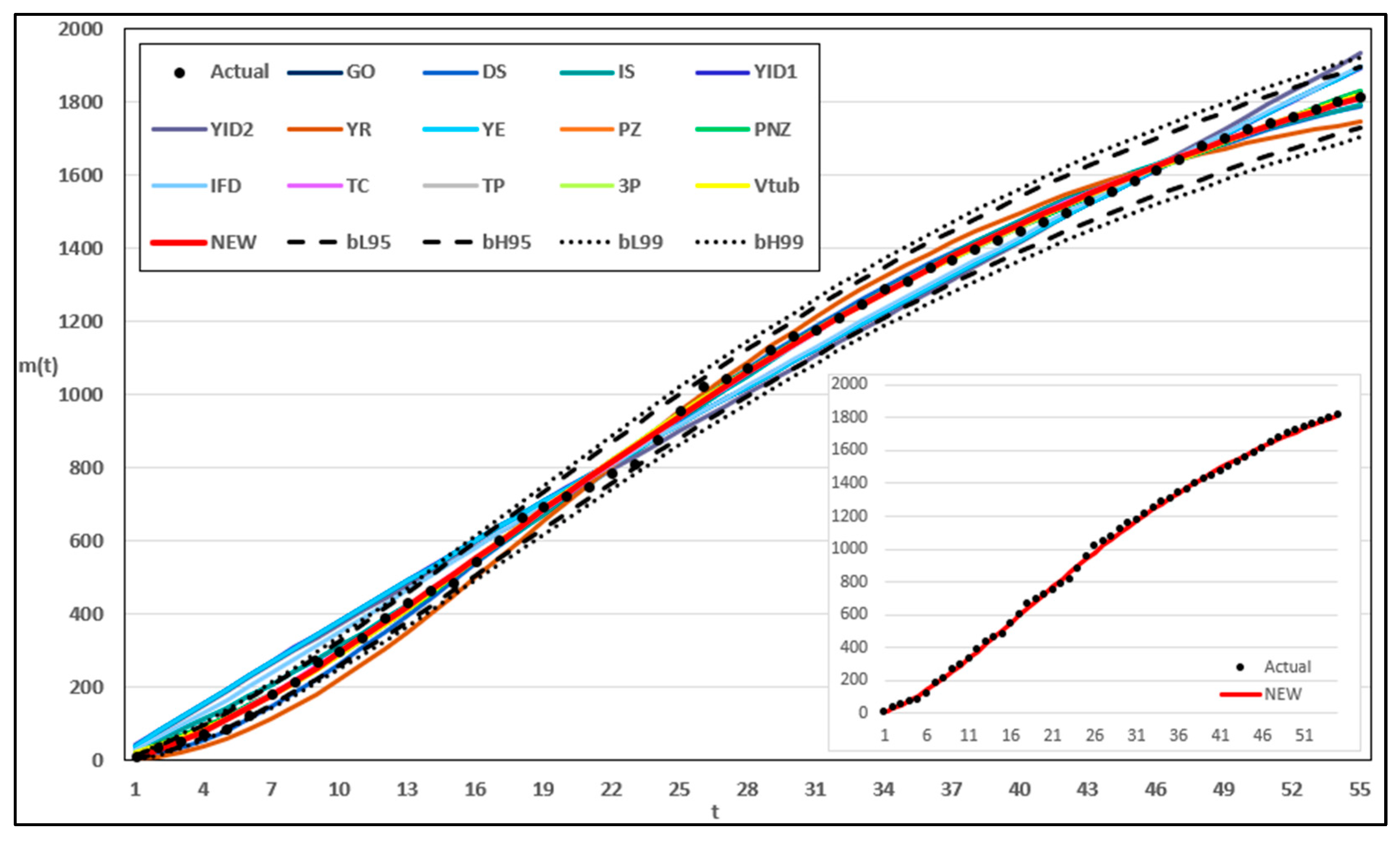
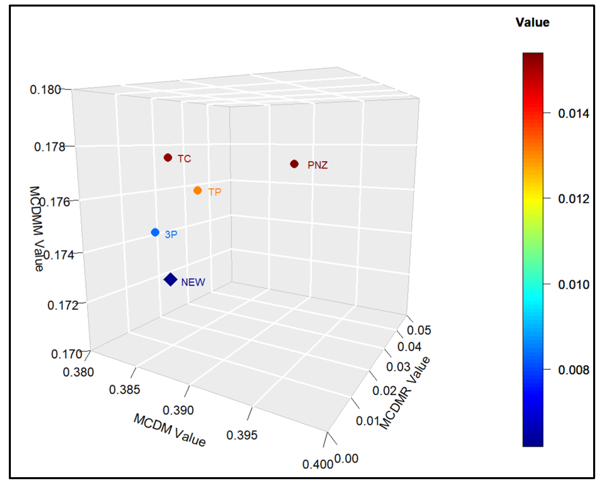
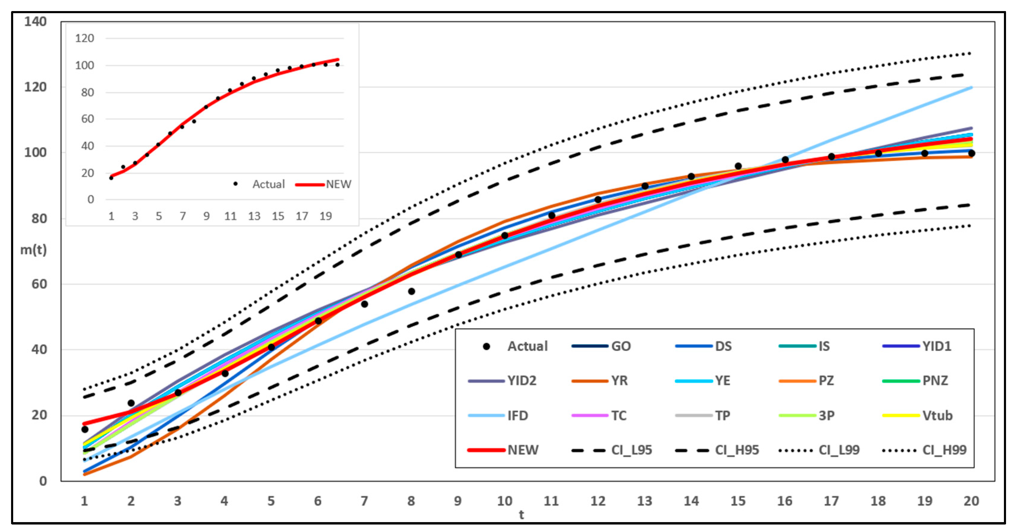
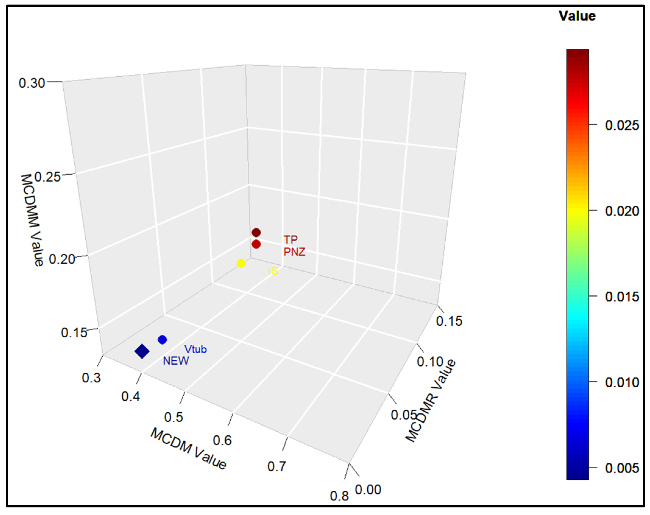
In this study, we extended the NHPP software reliability model to failures arising from complex software, thereby proposing an NHPP software reliability model that considers both operating environment uncertainty and dependent failure occurrence. Previously, proposed software reliability models were based on a single assumption. However, because software failures can be caused by various factors, we propose a software reliability model that includes the assumptions of dependent failure occurrence. This describes when failures affect each other, as well as the operating environment uncertainty caused by the difference between the development and operating environments. In addition, the software reliability was evaluated using various methods to determine the goodness of fit. However, because various criteria have different characteristics, evaluating excellence using only a few values is infeasible [26,27,28]. Therefore, we use a multi-criteria decision-making method ( M C D M ) for a comprehensive evaluation, demonstrating the effectiveness of the proposed model through the new M C D M , which reflects the size of the criteria for all models to be compared.
In summary, the contributions of this study are as follows:
  • This study proposes an NHPP software reliability model that considers both the uncertainty of the operating environment and dependent faults.
  • This study demonstrates the superiority of the proposed model through M C D M using the maximum value to approach comprehensive assessment and multi-faceted interpretation.
The remainder of this paper is organized as follows: Section 2 introduces the general NHPP software reliability model and the new NHPP software that considers dependent failures and operating environment uncertainties. Section 3 introduces the criteria and M C D M s used for model comparison and proposes a new M C D M . Section 4 presents the data and fit, along with numerical example results. Finally, Section 5 concludes the study.

2. New Software Reliability Model

2.1. Software Reliability Model

Software reliability assesses the ability of software to provide consistent results without faults. This is calculated using the reliability function R ( t ) , which is defined as the probability that it is still working after a certain point in time t . R ( t ) is equal to the result of integrating the probability density function f ( t ) with respect to the time of failure occurrence from t to infinity. The formula used is as follows:
R t = P ( T > t ) = t f u d u
To calculate the reliability function R ( t ) , we assumed a Poisson distribution with λ as the mean number of failures per unit time. Here, λ is a constant and follows a homogeneous poison process (HPP) with the number of failures per unit time constant over time. However, in real life, the number of software failures per unit time is time-dependent, which has led to the development of software reliability models that follow a nonhomogeneous Poisson process. NHPP is derived by using a mean value function m ( t ) , instead of the mean number of failures λ , based on the Poisson process [29,30].
P ( N t = n ) = { m ( t ) } n n ! e m ( t ) , n = 0,1 , 2 , , t 0
where N ( t ) is the number of failures up to time t , and mean value function m ( t ) is the mean number of failures from time 0 to t .

2.2. Proposed NHPP Software Reliability Model

Differential equations were used to derive the traditional NHPP software reliability model. The functions required to compute the NHPP software reliability model comprise those for the mean value function m ( t ) , number of failures a ( t ) , and failure detection rate function b ( t ) , which are derived using Equation (1), assuming that software failures occur independently [5].
d m ( t ) d t = b t [ a t m ( t ) ]
However, as software is utilized in various ways and its structure has become more complex, software failures typically depend on other failures, leading to failures in otherwise functioning software. In addition, as software utilization diversifies, the differences between software development and operating environments can result in software failure. Therefore, we propose a software reliability model for predicting and integrating multiple failures in diverse software applications. Previously, many software reliability studies assumed that software was independent, which is insufficient for describing complex software. Thus, research has been conducted on models that incorporate various assumptions, such as operating environment uncertainty and dependent failures. In this paper, we propose an NHPP software reliability model that considers both the uncertainty of the operating environment and dependent failures by extending a previously developed NHPP software reliability model. The differential equation for assuming operating environment uncertainty is expressed in Equation (2) [19].
d m ( t ) d t = η b t a t m t
where a ( t ) is the total expected number of failures N , and η follows a probability density function g generalized gamma distribution with shape parameter α and scale parameter β . When the initial value m 0 = 0 , the process derives the mean value function m t using Equation (3).
m t = η N 1 e x p η 0 t b x d x d g η
Furthermore, by defining b t = γ 2 t γ t + 1 and reorganizing Equation (3) using the Laplace transform, we obtain Equation (4) [31]:
m t = N 1 β γ + 0 t γ 2 s γ s + 1 d s α
where γ is the failure detection rate and is included in the denominator of Equation (4) and in the expression of b t = γ 2 t γ t + 1 . The assumption of operating environment uncertainty is also included in the failure detection rate γ , which assumes that dependent failures occurring in the operating environment are also considered. Therefore, the newly proposed NHPP software reliability model assumes both the dependent failure occurrence and operating environment uncertainty, as expressed in Equation (5).
m t = N 1 β γ + γ t l n γ t + 1 α
Table 1 lists the 15 NHPP software reliability models used in the study. Models 1–14 are traditional software reliability models with different assumptions of software failure, such as independent occurrence, dependent occurrence, and operating environment uncertainty. Model 15 is a new type of NHPP software reliability model proposed in this study, which considers both dependent failures and operating environment uncertainty.

3. New Criteria for Model Comparison

3.1. Criteria

To demonstrate the superiority of the proposed NHPP software reliability model, which simultaneously assumes dependent failures and operating environment uncertainty, we compared the proposed model with 14 traditional software reliability models using 13 criteria. These 13 criteria judge the superiority of the model based on the difference between the actual value y i and the estimated value m ^ t i . n and m are the number of observations and parameters in each model, respectively.
The mean squared error (MSE), mean absolute error (MAE), predictive ratio risk (PRR), and predictive power (PP) were based on the difference between the actual and predicted values, where PRR was determined by the ratio of the estimated value and PP was determined by the ratio of the actual value [32,33,34].
M S E = i = 1 n m ^ t i y i 2 n m ,   M A E = i = 1 n m ^ t i y i n m
P R R = i = 1 n m ^ t i y i m ^ t i 2 ,   P P = i = 1 n m ^ t i y i y i 2
R 2 and a d j _ R 2 are the coefficients of determination and the modified coefficient of determination of the regression equation, respectively [35].
R 2 = 1 i = 1 n m ^ t i y i 2 i = 1 n y i y i ¯ 2 ,   a d j _ R 2 = 1 1 R 2 n 1 n m 1
Akaike’s information criterion (AIC) and Bayesian information criterion (BIC) are used to compare the likelihood function maximization, as they aim to maximize the Kullback-Leibler level of agreement between the model and the probability distribution of the data, and BIC is a modified form of AIC [36]. The predicted relative variation (PRV) and root-mean-square prediction error (RMSPE) are the standard deviations of the prediction bias [37,38].
A I C = 2 log L + 2 m ,   B I C = 2 log L + m log n
P R V = i = 1 n y i m ^ t i i = 1 n m ^ t i y i n 2 n 1 ,
R M S P E = i = 1 n y i m ^ t i i = 1 n m ^ t i y i n 2 n 1 + i = 1 n m ^ t i y i n 2
The tail statistic (TS) is the average percentage deviation from the mean at all the time points. Pham’s information criterion (PIC) and Pham’s criterion (PC) consider the tradeoff between the number of parameters in the model by increasing the penalty for each additional parameter in the model when the sample is small. In particular, the PC includes a penalty for PIC [39,40,41].
T C = 100 × i = 1 n y i m ^ t i 2 i = 1 n y i 2 ,   P I C = i = 1 n m ^ t i y i 2 + m n 1 n m ,
P C = n m 2 × log i = 1 n m ^ t i y i 2 n + m n 1 n m
The proposed 13 criteria were used to judge the excellence of the model. The closer R 2 and a d j _ R 2 are to 1, the better the model; the closer the remaining 11 criteria are to 0, the better the model. The parameters of each model were estimated using MATLAB R2024b and R with the LSE method, and the criteria were calculated [42].

3.2. Existing Multicriteria Decision Method

In the past, researchers have compared criteria to demonstrate the superiority of the developed NHPP software reliability model. The criteria for comparison were the distance between the actual and estimated values or the actual and predicted values, whereby the shorter the distance, the better the model. However, various criteria with different characteristics make it difficult to judge whether a software reliability model is superior simply because only one criterion is superior. Therefore, complex assessment and multifaceted interpretations are required to determine the superiority of the NHPP software reliability model [43,44,45].
A multi-criteria decision method facilitates a comprehensive interpretation. In this study, we use M C D M to demonstrate the superiority of the proposed model by comparing multiple criteria. First, matrix C was constructed to compare the software reliability models based on the criteria calculated by the models, which are represented as follows:
C = C 11 C 12 C 21 C 22 C 1 k C 2 k C s 1 C s 2 C s k
From matrix C , we create a new matrix Y with components y i j for the objective criterion by normalizing each goodness of fit: y i j = C i j i = 1 s C i j ( i = 1,2 , , m ; j = 1,2 , , n ) , thereby summing the components in each row, to define M C D M with components S Y 1 to S Y s . The defined Y and M C D M are represented by Equation (7).
Y = y 11 y 12 y 21 y 22 y 1 k y 2 k y s 1 y s 2 y s k ,   M C D M = y 11 + y 12 + + y 1 k y 21 + y 22 + + y 2 k y s 1 + y s 2 + + y s k = S Y 1 S Y 2 S Y s
We compared the size of each component of the matrix M C D M such that the smaller the value, the better the overall model.

3.3. Multiple Criteria Decision Making Using Maximum

In M C D M , the most important issue is determining the weights based on fitness. Various methods exist for determining the weights, such as the Monte Carlo simulation, entropy, and the technique for performance by similarity with an ideal solution (TOPSIS). In particular, M C D M through ranking ( M C D M R ), which considers both quantitative and qualitative methods simultaneously, has been proposed [46]. However, because the weights were differentiated through ranking, even if the difference between the criteria of the two models was large, the difference in the reflected weights was the same. For instance, suppose that three random models have mean-squared error (MSE) values, as listed in Table 2. If the first model had an MSE of 100, the second had an MSE of 20, and the third had an MSE of 10, the difference in rank between the first and second models was 1, and the difference in MSE values was 80. The difference in rank between the second and third models was also one, but the difference in the MSE values was 10. The problem with simply reflecting the rankings is that if multiple models are equally spaced and perform well, a considerably small difference can result in a large penalty.
In this study, the previous problem was addressed using a multi-criteria decision method using maximum ( M C D M M ), which reflects the size of the criteria, instead of simply applying a ranking by dividing the values corresponding to the column criteria into ranges while computing the M C D M . Matrix M was constructed to utilize this size. The components of the matrix M are calculated by Equation (8) through w i j = C i j m a x C j ( i = 1,2 , , m , j = 1,2 , , n ) , where the maximum value of each criterion according to each model is distributed, utilizing the size.
M = w 11 w 12 w 21 w 22 w 1 k w 2 k w s 1 w s 2 w s k
The matrix Y M is defined by the product of the respective components of matrix M and matrix Y after the transformation process explained in 3.2, and follows from Equation (9).
Y M = w 11 y 11 w 12 y 12 w 21 y 21 w 22 y 22 w 1 k y 1 k w 2 k y 2 k w s 1 y s 1 w s 2 y s 2 w s k y s k
We define M C D M M by Equation (10) using Y M 1 to Y M s as the components that are summed in each row of the combined matrix Y M . The component sizes were compared to determine the overall excellence of the model based on smaller values.
M C D M M = w 11 y 11 + w 12 y 12 + + w 1 k y 1 k w 21 y 21 + w 22 y 22 + + w 2 k y 2 k w s 1 y s 1 + w s 2 y s 2 + + w s k y s k = Y M 1 Y M 2 Y M s
This study utilizes M C D M , which improves the existing method of judging the goodness of models, and proposes a new M C D M M that reflects the continuous value of criteria. We propose and utilize a new M C D M M to assess the goodness of fit of models with complex evaluations and multifaceted interpretations.

4. Numerical Example

4.1. Data Information

Two datasets are used to evaluate the effectiveness of the proposed model. The first dataset was the failure data from the PIG project, which is a platform for analyzing large datasets. The PIG project was used to display the parallelized data analysis programs. The PIG project has had five releases, with versions 0.2.0 through 0.5.0 defined as Release 1, versions 0.6.0 through 0.8.0 defined as Release 2, versions 0.8.1 through 0.9.2 defined as Release 3, version 0.10.0 defined as Release 4, and versions 0.10.1 through 0.12.0 defined as Release 5. A total of 1814 failures were observed monthly between April 2009 and October 2013 [47]. The second dataset comprises the failure data of a tandem computer with multiple central processing units inside a single computer. The system was tested for 10,000 h, and 100 failures occurred during testing. The data exhibited a concave shape with many failures at the beginning, followed by a gradual decrease [48].

4.2. Results of Dataset 1

Table 3 lists the estimated parameter values for each model obtained from dataset 1. In this study, the proposed model has four parameters: α , β , γ , and N , and the estimated values of dataset 1 are α ^ = 0.7342 , β ^ = 0.001093 , γ ^ = 0.001092 , and N ^ = 2594.496 . Figure 2 shows the cumulative number of failures and estimates for the 15 models at each time point from Dataset 1. The black dots represent the actual cumulative number of failures in Dataset 1, and the red line represents the estimated value of the software reliability model proposed in this study. Compared with the estimates of other existing software reliability models, the estimates of the proposed model are closest to the actual cumulative number of failures. In addition, the thick black dashed and thin black dotted lines represent the 95% and 99% confidence intervals of the proposed software reliability model, and all the actual values are within the confidence intervals.
Table 4 and Table 5 present the results for the calculated criteria and multi-criteria based on Table 3. M S E , R 2 , A d j _ R 2 , A I C , B I C , P R V , R M S P E , T S , and P I C have the best results, with 273.018, 0.999, 0.999, 518.486, 526.515, 16.057, 16.058, 1.393, and 13,928.1, respectively, whereas P P and M A E have the second-best results, with 0.351 and 13.483, respectively. The proposed model has the third-best result in M C D M with 0.3864 and the best results in M C D M R and M C D M M with 0.0062 and 0.1731, respectively. TC had the best result for M C D M but the fifth-best result for M C D M R and M C D M M . This demonstrates the importance of assigning weights for a comprehensive evaluation. Figure 3 is a graphical representation of the three-dimensional plots of the M C D M , M C D M R , and M C D M M for the top five of the 15 models listed in Table 1 for Dataset 1.

4.3. Results of Dataset 2

Table 6 lists the estimated parameters for the 15 models in Dataset 2. The estimated values are α ^ = 1.9561 , β ^ = 0.02901 , γ ^ = 0.04450 , and N ^ = 127.2589 . Figure 4 shows the cumulative number of failures and estimates for the 15 models at each time point in Dataset 2. The black dots represent the actual cumulative number of failures in Dataset 2, and the red line represents the estimates of the software reliability models from Dataset 2. The thick black dashed and thin black dotted lines represent the 95% and 99% confidence intervals of the proposed software reliability models, respectively. The estimated value of the proposed model was the closest to the true value compared to the results of the other models, and all were within the confidence interval of the true value.
Table 7 and Table 8 present the results for the calculated criteria and multi-criteria based on Table 6. M S E , M A E , P R R , P P , R 2 , A d j _ R 2 , P R V , R M S P E , T S , P C and P I C have the best values of 5.650, 0.040, 0.038, 2.075, 0.994, 0.993, 2.181, 2.181, 2.832, 16.818, and 95.153, respectively, whereas A I C and B I C have the second highest values of 88.732 and 92.715, respectively. The best results for M C D M , M C D M R , and M C D M M with the 13 criteria were 0.3906, 0.0043, and 0.1410, respectively. Figure 5 is a graphical representation of the three-dimensional plots of the M C D M , M C D M R , and M C D M M for the top five of the 15 models listed in Table 1 for Dataset 2.

4.4. Sensitivity Analysis

Because the software reliability model is highly sensitive to changes in the mean value function m ( t ) whenever the parameters change, this study compares the changes in the m ( t ) owing to changes in the four parameters through a sensitivity analysis [49,50]. In this study, we use two datasets to compare the most affected parameters of the mean value function m ( t ) when the parameters of the estimated model are varied by −20%, −10%, 10%, and 20%.
The changes in the four parameters of Dataset 1 are shown in Figure 6. For N and γ , the estimated mean value function m ( t ) became larger with increasing values, while for α and β , the m ( t ) became smaller with increasing values. Furthermore, the magnitude of the change in mean value function m ( t ) increased with increasing time point for N , γ gradually decreased, and β showed relatively small changes compared to the changes in other parameters.
The changes in the four parameters of Dataset 2 are shown in Figure 7. For N and γ, the estimated mean value function m(t) became larger with increasing values, while for α and β, m(t) became smaller with increasing values. For N, the variation in the mean value function m(t) increased as the time point increased, while α showed very small variation overall. γ and β showed very large variation initially but gradually became smaller.

5. Conclusions

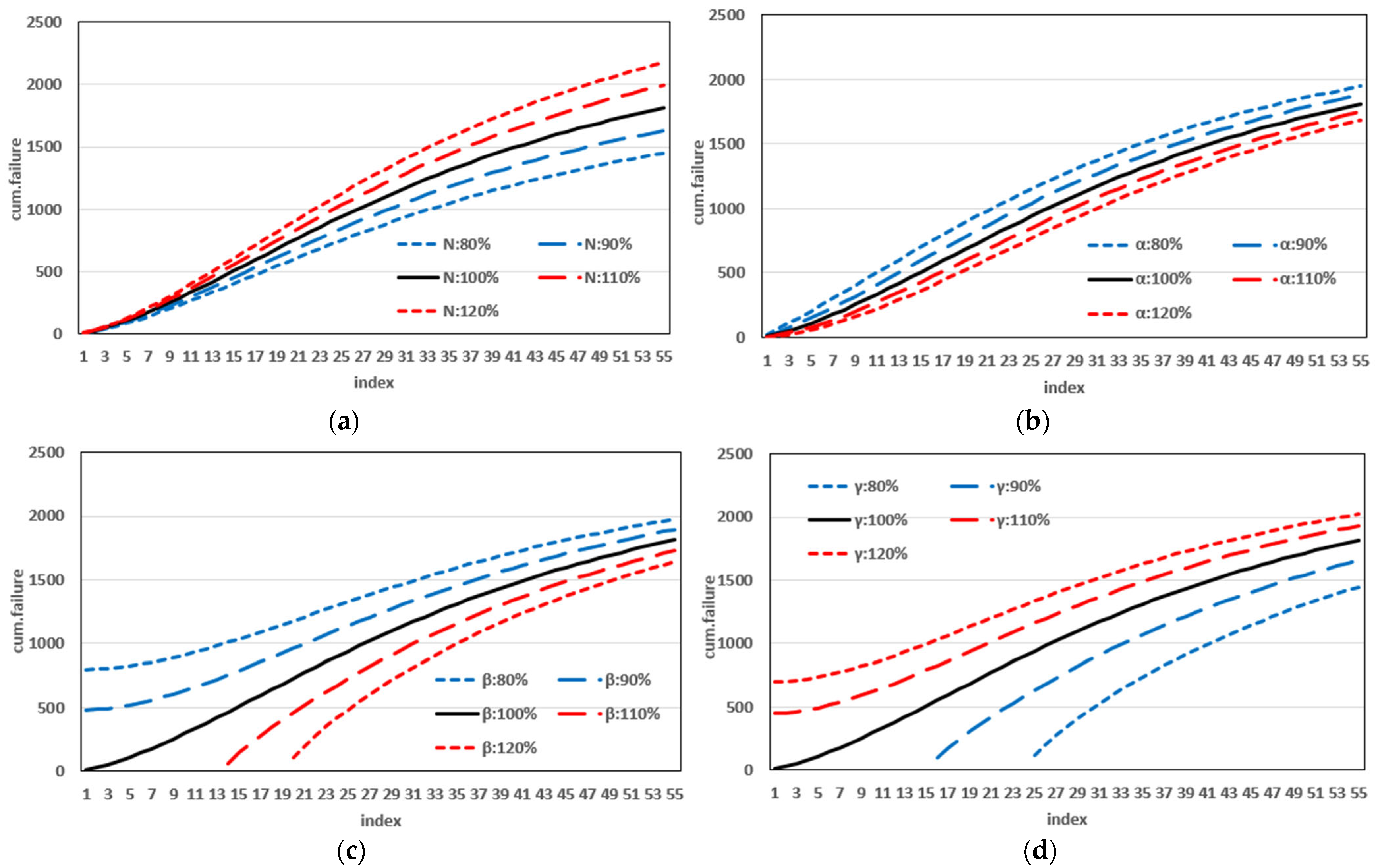
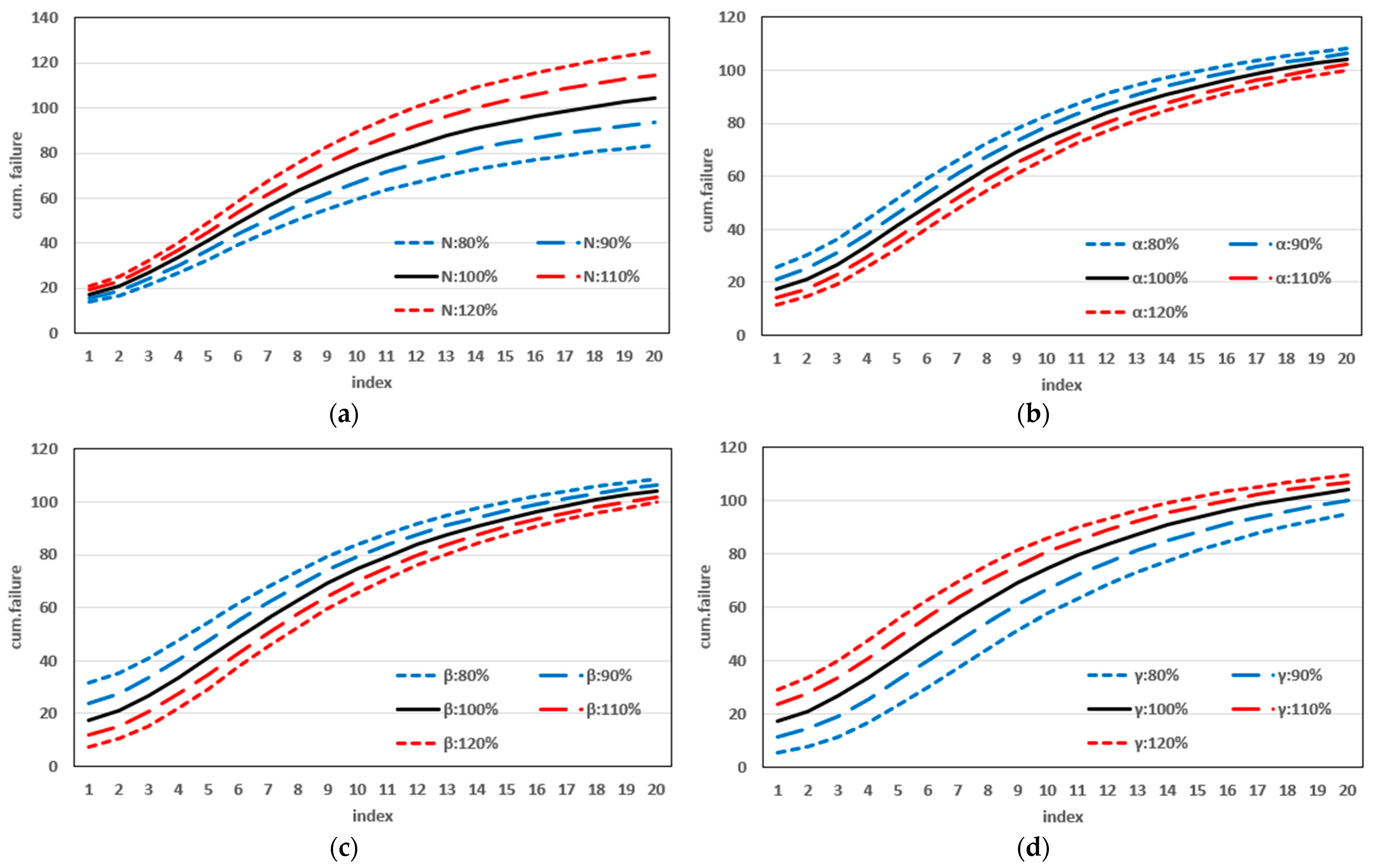
This study introduced a new type of NHPP software reliability model that simultaneously assumes uncertainty in the operating environment and dependent failure occurrence. Unlike previous studies, this study extends the range of failures that can occur in complex and diverse software by presenting a model that can predict the probability of occurrence in various environments. In addition, to demonstrate the effectiveness of the developed software reliability model, an M C D M using the maximum value, which can be interpreted in various manners. This method evaluates the effectiveness of a model through a comprehensive interpretation because when assessing the effectiveness of a model based on each criterion, it is particularly useful when multiple models perform well across individual criteria. In an analysis with 15 models across two datasets, it was showed that in Dataset 1, the proposed model performed best on all criteria, and in Dataset 2, the existing M C D M showed the third-best result, whereas the newly proposed M C D M M showed the best result. Therefore, the M C D M M , which improves the existing M C D M method, can increase the level of comparison by considering both quantitative and qualitative evaluations. The sensitivity analysis was conducted to compare the changes in the mean value function m t   due to changes in the parameters for the two datasets. The changes for N showed a trend of increasing variation as the value increases, α showed a relatively small variation compared to other parameters, and β showed a trend of decreasing variation as the value increases. The changes in the mean value function m t , that is, the impact on software failure prediction owing to changes in the parameters included in the model, varied per parameter and showed changes with common characteristics.
With the development of the software industry, the complexity and diversity of software have led to various software failures. Research on assumptions such as dependent failures and operating environment uncertainties is underway to predict these failures. Further research should be conducted based on additional assumptions to extend these studies. This study proposes a model with multiple assumptions, and there is a possibility of errors when these assumptions are changed. Therefore, additional research is required on generalizable software reliability models to predict software failure.

Author Contributions

Conceptualization, H.P.; Funding acquisition, Y.S.K. and K.Y.S.; Software, Y.S.K.; Writing—original draft, Y.S.K. and K.Y.S.; Writing—review and editing, K.Y.S., I.H.C. and H.P. All authors have read and agreed to the published version of the manuscript.

Funding

This research was supported by the Global-Learning & Academic Research Institution for Master’s and Ph.D. students and a Postdocs (LAMP) Program of the National Research Foundation of Korea (NRF) grant funded by the Ministry of Education (No. RS-2023-00285353).

Institutional Review Board Statement

Not applicable.

Informed Consent Statement

Not applicable.

Data Availability Statement

Data are available in a publicly accessible repository.

Acknowledgments

This study was supported by the National Research Foundation of Korea.

Conflicts of Interest

The authors declare no conflicts of interest.

References

  1. Cai, K.Y. On estimating the number of defects remaining in software. J. Syst. Softw. 1998, 40, 93–114. [Google Scholar] [CrossRef]
  2. Tohma, Y.; Yamano, H.; Ohba, M.; Jacoby, R. The estimation of parameters of the hypergeometric distribution and its application to the software reliability growth model. IEEE Trans. Softw. Eng. 1991, 17, 483. [Google Scholar] [CrossRef]
  3. Jelinski, Z.; Moranda, P.B. Software Reliability Research. In Statistical Computer Performance Evaluation; Academic Press: New York, NY, USA, 1972; pp. 465–484. [Google Scholar]
  4. Singpurwalla, N.D.; Wilson, S.P. Software reliability modeling. Int. Stat. Rev. 1994, 62, 289–317. [Google Scholar] [CrossRef]
  5. Goel, A.L.; Okumoto, K. Time-dependent error-detection rate model for software reliability and other performance measures. IEEE Trans. Reliab. 1979, 28, 206–211. [Google Scholar] [CrossRef]
  6. Hossain, S.A.; Dahiya, R.C. Estimating the parameters of a non-homogeneous Poisson-process model for software reliability. IEEE Trans. Reliab. 1993, 42, 604–612. [Google Scholar] [CrossRef]
  7. Yamada, S.; Ohba, M.; Osaki, S. S-shaped reliability growth modeling for software fault detection. IEEE Trans. Reliab. 1983, 32, 475–484. [Google Scholar] [CrossRef]
  8. Ohba, M. Inflection S-shaped software reliability growth model. In Stochastic Models in Reliability Theory; Springer: Berlin/Heidelberg, Germany, 1984; pp. 144–162. [Google Scholar]
  9. Yamada, S.; Tokuno, K.; Osaki, S. Imperfect debugging models with fault introduction rate for software reliability assessment. Int. J. Syst. Sci. 1992, 23, 2241–2252. [Google Scholar] [CrossRef]
  10. Yamada, S.; Ohtera, H.; Narihisa, H. Software Reliability Growth Models with Testing-Effort. IEEE Trans. Reliab. 1986, 35, 19–23. [Google Scholar] [CrossRef]
  11. Roy, P.; Mahapatra, G.S.; Dey, K.N. An NHPP software reliability growth model with imperfect debugging and error generation. Int. J. Reliab. Qual. Saf. Eng. 2014, 21, 1–32. [Google Scholar] [CrossRef]
  12. Pham, H.; Zhang, X. An NHPP software reliability models and its comparison. Int. J. Reliab. Qual. Saf. Eng. 1997, 4, 269–282. [Google Scholar] [CrossRef]
  13. Pham, H.; Nordmann, L.; Zhang, X. A general imperfect software debugging model with S-shaped fault detection rate. IEEE Trans. Reliab. 1999, 48, 169–175. [Google Scholar] [CrossRef]
  14. Yang, T.J. Comparative study on the performance attributes of NHPP software reliability model based on Weibull family distribution. Int. J. Perform. Eng. 2021, 17, 343. [Google Scholar] [CrossRef]
  15. Nafreen, M.; Fiondella, L. A family of software reliability models with bathtub-shaped fault detection rate. Int. J. Reliab. Qual. Saf. Eng. 2021, 28, 2150034. [Google Scholar] [CrossRef]
  16. Li, Q.; Pham, H. Modeling Software Fault-Detection and Fault-Correction Processes by Considering the Dependencies between Fault Amounts. Appl. Sci. 2021, 11, 6998. [Google Scholar] [CrossRef]
  17. Pan, Z.; Nonaka, Y. Importance analysis for the systems with common cause failures. Reliab. Eng. Syst. Saf. 1995, 50, 297–300. [Google Scholar] [CrossRef]
  18. Teng, X.; Pham, H. A new methodology for predicting software reliability in the random field environments. IEEE Trans. Reliab. 2006, 55, 458–468. [Google Scholar] [CrossRef]
  19. Pham, H. A new software reliability model with Vtub-Shaped fault detection rate and the uncertainty of operating environments. Optimization 2014, 63, 1481–1490. [Google Scholar] [CrossRef]
  20. Chang, I.H.; Pham, H.; Lee, S.W.; Song, K.Y. A testing-coverage software reliability model with the uncertainty of operation environments. Int. J. Syst. Sci. Oper. Logist. 2014, 1, 220–227. [Google Scholar]
  21. Song, K.Y.; Chang, I.H.; Pham, H. A Three-parameter fault-detection software reliability model with the uncertainty of operating environments. J. Syst. Sci. Syst. Eng. 2017, 26, 121–132. [Google Scholar] [CrossRef]
  22. Pradhan, V.; Dhar, J.; Kumar, A. Testing coverage-based software reliability growth model considering uncertainty of operating environment. Syst. Eng. 2023, 26, 449–462. [Google Scholar] [CrossRef]
  23. Haque, M.A.; Ahmad, N. Software reliability modeling under an uncertain testing environment. Int. J. Model. Simul. 2025, 45, 321–327. [Google Scholar] [CrossRef]
  24. Liu, Z.; Yang, S.; Yang, M.; Kang, R. Software belief reliability growth model based on uncertain differential equation. IEEE Trans. Reliab. 2022, 71, 775–787. [Google Scholar] [CrossRef]
  25. Zheng, Z.; Yang, J.; Huang, J. Software-hardware embedded system reliability modeling with failure dependency and masked data. Comput. Ind. Eng. 2023, 186, 109746. [Google Scholar] [CrossRef]
  26. Kagazyo, T.; Kaneko, K.; Akai, M.; Hijikata, K. Methodology and evaluation of priorities for energy and environmental research projects. Energy 1997, 22, 121–129. [Google Scholar] [CrossRef]
  27. Ulutaş, B.H. Determination of the appropriate energy policy for Turkey. Energy 2005, 30, 1146–1161. [Google Scholar] [CrossRef]
  28. Boran, F.E.; Etöz, M.; Dizdar, E. Is nuclear power an optimal option for electricity generation in Turkey? Energy Sources Part B 2013, 8, 382–390. [Google Scholar] [CrossRef]
  29. Willis, D.M. The statistics of a particular non-homogeneous Poisson process. Biometrika 1964, 51, 399–404. [Google Scholar] [CrossRef]
  30. Cai, K.Y.; Wen, C.Y.; Zhang, M.L. A critical review on software reliability modeling. Reliab. Eng. Syst. Saf. 1991, 32, 357–371. [Google Scholar] [CrossRef]
  31. Spiegel, M.R. Laplace Transforms; McGraw-Hill: New York, NY, USA, 1965. [Google Scholar]
  32. Armstrong, J.S.; Collopy, F. Error Measures for Generalizing about Forecasting Methods: Empirical Comparisons. Int. J. Forecast. 1992, 8, 69–80. [Google Scholar] [CrossRef]
  33. Willmott, C.; Matsuura, K. Advantages of the Mean Absolute Error (MAE) over the Root Mean Square Error (RMSE) in Assessing Average Model Performance. Clim. Res. 2005, 30, 79–82. [Google Scholar] [CrossRef]
  34. Iqbal, J. Software Reliability Growth Models: A Comparison of Linear and Exponential Fault Content Functions for Study of Imperfect Debugging Situations. Cogent Eng. 2017, 4, 1286739. [Google Scholar] [CrossRef]
  35. Akossou, A.Y.J.; Palm, R. Impact of Data Structure on the Estimators R-Square and Adjusted R-Square in Linear Regression. Int. J. Math. Comput. 2013, 20, 84–93. [Google Scholar]
  36. Kuha, J. AIC and BIC: Comparisons of Assumptions and Performance. Sociol. Methods Res. 2004, 33, 188–229. [Google Scholar] [CrossRef]
  37. Xu, J.; Yao, S. Software Reliability Growth Model with Partial Differential Equation for Various Debugging Processes. Math. Probl. Eng. 2016, 2016, 1–13. [Google Scholar] [CrossRef]
  38. Witt, S.F.; Witt, C.A. Modeling and Forecasting Demand in Tourism; Academic Press Ltd.: Cambridge, MA, USA, 1992. [Google Scholar]
  39. Sharma, K.; Garg, R.; Nagpal, C.K.; Garg, R.K. Selection of Optimal Software Reliability Growth Models Using a Distance Based Approach. IEEE Trans. Reliab. 2010, 59, 266–276. [Google Scholar] [CrossRef]
  40. Ali, N.N. A Comparison of Some Information Criteria to Select a Weather Forecast Model. Turk. J. Comput. Math. Educ. (TURCOMAT) 2021, 12, 2494–2500. [Google Scholar]
  41. Pham, H. On Estimating the Number of Deaths Related to COVID-19. Mathematics 2020, 8, 655. [Google Scholar] [CrossRef]
  42. Wang, L.; Hu, Q.; Liu, J. Software Reliability Growth Modeling and Analysis with Dual Fault Detection and Correction Processes. IIE Trans. 2016, 48, 359–370. [Google Scholar] [CrossRef]
  43. Pujadas, P.; Pardo-Bosch, F.; Aguado-Renter, A.; Aguado, A. MIVES multi-criteria approach for the evaluation, prioritization, and selection of public investment projects. A case study in the city of Barcelona. Land Use Policy 2017, 64, 29–37. [Google Scholar] [CrossRef]
  44. Del Cano, A.; Gomez, D.; de la Cruz, M.P. Uncertainty analysis in the sustainable design of concrete structures: A probabilistic method. Constr. Build. Mater. 2012, 37, 865–873. [Google Scholar] [CrossRef]
  45. Alhumaid, M.; Ghumman, A.R.; Haider, H.; Al-Salamah, I.S.; Ghazaw, Y.M. Sustainability Evaluation Framework of Urban Stormwater Drainage Options for Arid Environments Using Hydraulic Modeling and Multicriteria Decision-Making. Water 2018, 10, 581. [Google Scholar] [CrossRef]
  46. Song, K.Y.; Kim, Y.S.; Pham, H.; Chang, I.H. A Software Reliability Model Considering a Scale Parameter of the Uncertainty and a New Criterion. Mathematics 2024, 12, 1641. [Google Scholar] [CrossRef]
  47. Tandon, A.; Sharma, M.; Kumari, M.; Singh, V.B. Entropy based software reliability growth modelling for open source software evolution. Teh. Vjesn. 2020, 27, 550–557. [Google Scholar]
  48. Wood, A. Predicting software reliability. IEEE Comput. Soc. 1996, 11, 69–77. [Google Scholar] [CrossRef]
  49. Xie, M.; Shen, K. On ranking of system components with respect to different improvement actions. Microelectron. Reliab. 1989, 29, 159–164. [Google Scholar] [CrossRef]
  50. Li, X.; Xie, M.; Ng, S.H. Sensitivity analysis of release time of software reliability models incorporating testing effort with multiple change-points. Appl. Math. Model. 2010, 34, 3560–3570. [Google Scholar] [CrossRef]
Figure 1. Software reliability model Methodology.
Applsci 15 05184 g001
Figure 2. Prediction of all models for dataset 1.
Applsci 15 05184 g002
Figure 3. Three-dimensional plot of the M C D M , M C D M R , and M C D M M for Dataset 1.
Applsci 15 05184 g003
Figure 4. Prediction of all models for Dataset 2.
Applsci 15 05184 g004
Figure 5. Three-dimensional plot of the M C D M , M C D M R , and M C D M M for Dataset 2.
Applsci 15 05184 g005
Figure 6. Results of sensitivity analysis for changes in parameters in dataset 1. (a) parameter N; (b) parameter α; (c) parameter β; (d) parameter γ.
Applsci 15 05184 g006
Figure 7. Results of sensitivity analysis for changes in parameters in dataset 2. (a) parameter N ; (b) parameter α ; (c) parameter β ; (d) parameter γ .
Applsci 15 05184 g007
Table 1. Software reliability models.
No.ModelMean Value FunctionNote
1Goel-Okumoto (GO) [5] m t = a 1 e b t Concave
2Yamada et al. (DS) [7] m t = a 1 1 + b t e b t S-Shape
3Ohba (IS) [8] m t = a t 1 e b t 1 + β e b t S-Shape
4Yamada et al. (YID 1) [9] m t = a b α + b e α t e b t Concave
5Yamada et al. (YID 2) [9] m t = a 1 e b t 1 α b + α a t Concave
6Yamada et al. (YR) [10] m t = a 1 e γ α 1 e β t 2 / 2 S-Shape
7Yamada et al. (YE) [10] m t = a 1 e γ α 1 e β t Concave
8Pham-Zhang (PZ) [12] m t = ( c + a 1 e b t a b b α e a t e b t ) 1 + β e b t Both
9Pham et al. (PNZ) [13] m t = a 1 e b t 1 α b + α a t 1 + β e b t Both
10Pham (IFD) [26] m t = a 1 e b t 1 + b + d t + b d t 2 Concave
11Chang et al. (TC) [20] m t = N 1 β β + a t b α Both
12Teng-Pham (TP) [18] m t = a p q 1 β β + p q ln c + e b t c + 1 α S-Shape
13Song et al. (3P) [21] m t = N 1 β β a b ln 1 + c e b t 1 + c e b t S-Shape
14Pham (Vtub) [19] m t = N 1 β β + a b t 1 α S-Shape
15Proposed Model m t = N 1 β γ + γ t l n γ t + 1 α S-Shape
Table 2. Examples of M C D M .
ModelMSERankWeight-RankWeight-Max
Model 110030.501.0
Model 22020.330.2
Model 31010.170.1
Table 3. Parameter estimation of model from Dataset 1.
No.Model a ^ b ^ α ^ β ^ N ^ γ ^ c ^ p ^ q ^ d ^
1GO8874.7380.004367
2DS2116.2710.060638
3IS2006.6430.070081 4.556844
4YID18381.190.0046427.73 × 10−5
5YID2437.53060.0877850.078345
6YR2269.766 0.9235090.001184 1.905442
7YE8911.425 0.6192141.94 × 10−5 362.1234
8PZ162,359.50.1184370.0001344.351755 836.2331
9PNZ839.14320.1183760.0256884.364091
10IFD368.7350.076678 4.22 × 10⁻⁷
11TC0.0002211.4751817509.9446.1426952155.745
12TP301.23890.1821611.1375920.847396 3.5083690.0876440.005934
133P0.3158120.18365 16.455983854.995 3.561905
14Vtub2.1094970.6171140.14828223.856923197.256
15NEW 0.7342140.0010932594.4960.001092
Table 4. Comparison of criteria from Dataset 1.
ModelMSEPRRPPMAER2adj_R2AICBICPRVRMSPETSPCPIC
GO3017.7752.42614.21847.5330.9910.991636.406640.42052.68054.3924.720213.381159,944.1
DS539.9606.2141.13720.5790.9980.998532.665536.67922.46323.0111.996167.78128,619.9
IS587.3841.0313.51620.7490.9980.998544.631550.65323.50123.7782.062167.42530,547.1
YID13078.1982.44314.38948.4990.9910.991637.655643.67752.60654.4124.721210.492160,069.4
YID23699.7822.33913.48053.1370.9890.989667.306673.32859.05859.6775.176215.274192,391.8
YR2216.82224.1912.54542.8120.9940.993620.157628.18743.89145.7233.968198.758113,062.1
YE3136.4042.42714.23049.3950.9910.990640.449648.47852.62254.3944.720207.606159,960.8
PZ285.2070.4471.00413.5430.9990.999527.946537.98216.22216.2501.409144.34814,265.7
PNZ279.6790.4481.00613.2770.9990.999525.986534.01516.22316.2521.409145.96814,267.9
IFD1883.5161.6106.33837.8860.9950.994593.414599.43641.88542.5763.693197.72097,945.9
TC302.3820.1350.18914.5020.9990.999518.597528.63416.72016.7331.451145.81015,124.5
TP293.3650.3050.58414.3010.9990.999525.980540.03116.13616.1481.400140.96214,089.4
3P281.6140.2970.56313.6980.9990.999521.957531.99416.13716.1481.400144.03114,086.1
Vtub287.9740.4431.20814.1270.9990.999524.983535.02016.31316.3291.416144.58914,404.1
NEW273.0180.6940.35113.4830.9990.999518.486526.51516.05716.0581.393145.35313,928.1
Table 5. Comparison of multi-criteria from dataset 1.
Multi-criteriaGODSISYID1YID2YRYEPZPNZIFDTCTP3PVtubNEW
M C D M 1.53820.64580.57991.54891.71411.61661.55430.39560.39471.07140.38330.38700.38420.39980.3864
M C D M R 0.16420.05000.04400.17820.21660.16930.17880.01520.01540.09270.01530.01310.00840.01620.0062
M C D M M 1.32850.27750.26521.34641.65621.30581.35560.17800.17740.68150.17750.17630.17470.17850.1731
Table 6. Parameter estimation of model from Dataset 2.
NoModel a ^ b ^ α ^ β ^ N ^ γ ^ c ^ p ^ q ^ d ^
1GO130.20150.083166
2DS103.98420.265379
3IS110.82870.172063 1.204647
4YID1129.80170.083450.000146
5YID272.353010.1694620.036291
6YR115.816 1.5654340.017194 1.268592
7YE130.4047 0.6574080.000264 478.892
8PZ0.2534690.1720631846.2881.204651 110.5752
9PNZ110.80990.1720839.88 × 10−61.204507
10IFD12.229180.440572 8.20 × 10⁻⁷
11TC0.0181831.10973386,418.8413,230.13118.5624
12TP90.281510.08819125.762771.159252 19.257390.956040.092387
133P1.3985670.172062 0.00897110.8898 1997.82
14Vtub3.7610850.4209117.023092169.2326105.9848
15NEW 1.9560810.029012127.25890.044502
Table 7. Comparison of criteria from Dataset 2.
ModelMSEPRRPPMAER2adj_R2AICBICPRVRMSPETSPCPIC
GO12.9080.3780.2033.4050.9860.98491.95993.9513.4963.4974.54024.183234.453
DS28.06319.5801.0813.5200.9690.965111.228113.2204.9465.1466.69431.173507.239
IS10.5640.8680.3052.6590.9890.98790.26693.2533.0423.0733.99122.010182.937
YID113.6880.3780.2033.6090.9860.98393.98496.9713.4983.5004.54424.212236.054
YID220.2640.2500.1884.4830.9790.97599.356102.3434.2574.2585.52827.547347.844
YR49.42157.1781.4975.5190.9510.938128.759132.7426.1106.4358.37534.168795.482
YE14.5390.3780.2033.8340.9860.98295.97699.9593.4983.4994.54324.379237.366
PZ11.9720.8680.3053.0140.9890.98594.26699.2453.0423.0733.99122.795185.918
PNZ11.2250.8670.3052.8260.9890.98692.26996.2523.0423.0733.99222.310184.354
IFD95.2953.3690.8519.4110.9000.882124.499127.4878.6639.20611.98840.7061623.369
TC14.4940.8300.3003.6000.9870.98297.871102.8493.3673.3824.39224.229223.750
TP11.9440.8630.3012.9550.9900.98595.356102.3262.8192.8573.71123.552165.504
3P11.9720.8680.3053.0140.9890.98594.26699.2453.0423.0733.99122.795185.918
Vtub6.8690.2390.1372.3460.9940.99187.50092.4792.2912.3273.02318.628109.369
NEW5.6500.0400.0382.0750.9940.99388.73292.7152.1812.1812.83216.81895.153
Table 8. Comparison of multi-criteria from Dataset 2.
Multi-CriteriaGODSISYID1YID2YRYEPZPNZIFDTCTP3PVtubNEW
M C D M 0.63351.32130.57800.64590.79632.19610.65930.60270.58962.29360.66700.58650.60270.43700.3906
M C D M R 0.04030.14790.01980.04940.07870.27210.05550.03050.02790.28890.05230.02940.03060.00640.0043
M C D M M 0.24500.67510.20840.25410.35221.74090.26430.22630.21672.19200.26440.22270.22630.15300.1410
Disclaimer/Publisher’s Note: The statements, opinions and data contained in all publications are solely those of the individual author(s) and contributor(s) and not of MDPI and/or the editor(s). MDPI and/or the editor(s) disclaim responsibility for any injury to people or property resulting from any ideas, methods, instructions or products referred to in the content.

