Rough Set Theory and Soft Computing Methods for Building Explainable and Interpretable AI/ML Models

Abstract

This study introduces a novel framework leveraging Rough Set Theory (RST)-based feature selection—MLReduct, MLSpecialReduct, and MLFuzzyRoughSet—to enhance machine learning performance on uncertain data. Applied to a private cardiovascular dataset, our MLSpecialReduct algorithm achieves a peak Random Forest accuracy of 0.99 (versus 0.85 without feature selection), while MLFuzzyRoughSet improves accuracy to 0.83, surpassing our MLVarianceThreshold (0.72–0.77), an adaptation of the traditional VarianceThreshold method. We integrate these RST techniques with preprocessing (discretization, normalization, encoding) and compare them against traditional approaches across classifiers like Random Forest and Naive Bayes. The results underscore RST’s edge in accuracy, efficiency, and interpretability, with MLSpecialReduct leading in minimal attribute reduction. Against baseline classifiers without feature selection and MLVarianceThreshold, our framework delivers significant improvements, establishing RST as a vital tool for explainable AI (XAI) in healthcare diagnostics and IoT systems. These findings open avenues for future hybrid RST-ML models, providing a robust, interpretable solution for complex data challenges.

1. Introduction

1.1. Context

In an era where data drive innovation, Rough Set Theory (RST) offers a powerful foundation for tackling uncertain and complex datasets. This study harnesses RST-based methods to advance feature selection in machine learning workflows. Initially developed by Zdzislaw Pawlak in the early 1980s, RST excels in identifying hidden patterns within incomplete, imprecise, or uncertain datasets, making it indispensable for modern intelligent systems and knowledge discovery tasks [1,2]. Unlike traditional methods that often struggle with non-linear or missing data, RST provides a structured and robust approach [3], enabling the extraction of decision rules from both qualitative and quantitative data [4].

What sets RST apart is its inherent ability to process and interpret imperfect data without requiring additional assumptions or information [5]. This makes RST particularly effective in tasks such as feature selection, discretization, and decision rule induction. Its flexibility allows it to adapt to various machine learning (ML) and data preprocessing scenarios [6], rendering it indispensable for tasks that require handling uncertainty or incomplete data. In this evolving landscape, RST is recognized as a versatile and essential tool in the pursuit of intelligent data analysis [7,8].

1.2. Problematic

As datasets grow in complexity and machine learning spans diverse domains, advanced feature selection becomes essential [9]. Traditional methods like VarianceThreshold struggle with uncertain, imbalanced, or large-scale data, leading to overfitting and inefficiency [10]. This study addresses the integration of RST-based feature selection—MLReduct, MLSpecialReduct, and MLFuzzyRoughSet [11,12]—into ML workflows to enhance classifier performance, such as with XGBoost [13], surpassing the limitations of our adapted MLVarianceThreshold [14].

1.3. Contribution

This paper presents a novel framework based on Rough Set Theory (RST) for feature selection, designed to enhance machine learning classifiers under uncertain and complex data conditions. Our work advances RST-based feature selection through three key innovations:

• Advanced RST Methods: We introduce three RST-based algorithms—MLReduct, MLSpecialReduct, and MLFuzzyRoughSet—that outperform traditional methods like MLVarianceThreshold. MLSpecialReduct, in particular, achieves minimal attribute reduction while maintaining high accuracy.
• Dynamic Dependency Optimization: MLSpecialReduct uniquely combines incremental attribute evaluation with real-time redundancy checks, eliminating the need for postprocessing.
• Hybrid Fuzzy Rough Handling: MLFuzzyRoughSet introduces adaptive membership thresholds (Section 5.3.5), automatically tuning $\alpha$-cuts based on data distribution.
• Computational Efficiency: Our methods achieve 12% higher accuracy than tri-level reducts [15] while reducing runtime by 3× (Section 5.4).
• Statistical Robustness: All results include 10-fold cross-validation with p < 0.01 significance.
• Broad Applicability: Validated on both private clinical data and public benchmarks (Section 5.5).

1.4. Paper Organization

This paper is structured as follows: Section 2 surveys the RST-based feature selection literature. Section 3 outlines Rough Set Theory (RST) foundations and its modern applications in feature selection. Section 4 details our methodology, including MLReduct, MLSpecialReduct, and MLFuzzyRoughSet implementations. Section 5 presents experimental results, and Section 6 summarizes findings and future research directions.

2. Related Work

Rough Set Theory (RST) has been widely applied across various domains, demonstrating its effectiveness in handling imperfect and uncertain data. Below, we review key studies that have contributed to the development and application of RST, particularly in feature selection, classification, and real-world applications.

2.1. Related Works

• Tri-level Attribute Reduction in Rough Set Theory: Zhang and Yao (2022) introduced a tri-level attribute reduction framework, extending traditional attribute reduction by incorporating object-specific reducts at the micro-bottom level. This approach enhances both classification-specific and class-specific reducts, providing a more granular and hierarchical understanding of attribute reduction in Rough Set Theory [15].
• Seasonal Air Quality Prediction using Regularized Combinational LSTM: In a study by Manna et al., 2023, a framework for predicting air quality seasonally using Regularized Combinational LSTM (REG-CLSTM) was proposed. The model aims to improve air quality prediction accuracy and reduce error rates by leveraging a large real-time dataset. The study employed a rough set-wrapper method for significant feature extraction and addressed the challenge of providing seasonal limit ranges for pollutants. The proposed pyramid learning-based hybridized deep learning framework can play a crucial role in warning policymakers to reduce activities that contribute to air pollution [16].
• Financial Risk Early Warning Model: Liu and Yang (2024) developed a financial risk early warning model for listed companies using Rough Set Theory and a BP neural network. Their model achieved high accuracy, recall, and F1-scores, demonstrating its effectiveness in predicting financial risks and providing decision support for financial management [17].
• Boundary-wise Loss using Fuzzy Rough Sets: In a study by Lin et al., 2024, a novel boundary-wise loss function for medical image segmentation was proposed, leveraging fuzzy rough sets. The loss function, based on the lower approximation of fuzzy rough sets, focuses on improving the delineation of object boundaries in semantic segmentation. Experiments demonstrated that the proposed loss outperforms traditional pixel-wise and region-wise losses in terms of Hausdorff distance and symmetric surface distance, while maintaining competitive performance in Dice coefficient and pixel-wise accuracy. The study highlights the importance of boundary-wise loss in producing more accurate shapes of segmented objects [18].
• Rough Set Theory in Vector Spaces: Fatima and Javaid (2024) explored the application of Rough Set Theory to finite-dimensional vector spaces. They defined an indiscernibility relation and studied partitions, reducts, and dependency measures, providing a theoretical foundation for applying RST in linear algebra contexts [19].
• Intelligent Recommender System for Disease Prediction: Singh and Mantri (2024) proposed a hybrid recommender system using machine learning association rules and Rough Set Theory for disease prediction from incomplete symptom sets. Their system achieved high accuracy and precision, particularly in detecting neurodevelopmental diseases [20].
• Student Performance Prediction: Nayani and Rao (2025) developed a hybrid deep learning model combined with entropy-weighted rough set feature mining for predicting student performance. Their approach, which optimizes hyperparameters using a Galactic Rider Swarm Optimization algorithm, achieved high sensitivity and accuracy rates [21].

To provide a clear overview of the related works, Table 1 summarizes the key studies, their contributions, and the domains in which they were applied.

Table 1. Comparison of related works in Rough Set Theory.

Study	Contribution	Key Findings
Zhang and Yao (2022) [15]	Tri-level attribute reduction	Introduced object-specific reducts for granular attribute reduction in data analysis.
Manna et al. (2024) [16]	Seasonal air quality prediction using REG-CLSTM	Proposed a hybridized deep learning framework for seasonal air quality prediction, leveraging rough set-wrapper methods for feature extraction and identifying seasonal pollutant trends.
Liu and Yang (2024) [17]	Financial risk early warning	Achieved high accuracy in financial risk prediction using RST and BP neural networks.
Lin et al. (2024) [18]	Boundary-wise loss using fuzzy rough sets	Introduced a boundary-wise loss function for medical image segmentation, improving boundary delineation and outperforming traditional losses in Hausdorff distance and symmetric surface distance.
Fatima and Javaid (2024) [19]	RST in vector spaces	Provided theoretical foundations for applying RST in finite-dimensional vector spaces.
Singh and Mantri (2024) [20]	Disease prediction	Achieved high accuracy in predicting neurodevelopmental diseases using RST and machine learning.
Nayani and Rao (2025) [21]	Student performance prediction	Optimized feature mining using entropy-weighted RST for predicting student performance in education.

2.2. Novelty of Our Work

While prior studies have advanced Rough Set Theory (RST) across domains, our work presents a unified RST-based feature selection framework—MLReduct, MLSpecialReduct, and MLFuzzyRoughSet—to optimize machine learning under uncertainty. Unlike traditional methods like PCA, RFE, and our adapted MLVarianceThreshold, which struggle with complex, noisy data due to statistical oversimplification, our RST techniques overcome these limitations. Below, we explicitly outline the novel contributions of our proposed methods and how they differ from existing RST-based feature selection techniques:

• MLReduct:

  –

  Novelty: MLReduct introduces a systematic approach to identifying minimal attribute subsets (reducts) that preserve the positive region of the full attribute set. Unlike traditional reduct algorithms, MLReduct employs an exhaustive search combined with a positive region preservation criterion, ensuring that the selected features maintain the classification power of the original dataset.

  –

  Advantage over Existing Methods: While existing reduct algorithms often rely on heuristic or greedy search strategies, MLReduct ensures optimality by evaluating all possible attribute combinations. This makes it particularly effective for datasets where attribute dependencies are complex and non-linear.

• MLSpecialReduct:

  –

  Novelty: MLSpecialReduct is a dynamic, dependency-driven feature selection method that iteratively builds a reduct by maximizing the dependency between the selected attributes and the decision attribute. It stops when the dependency matches that of the full attribute set or no further improvement is possible.

  –

  Advantage over Existing Methods: Unlike traditional dependency-based reduct algorithms, MLSpecialReduct dynamically optimizes the attribute selection process, ensuring minimal redundancy and maximal relevance. This makes it highly efficient for high-dimensional datasets where traditional methods may fail to scale.

• MLFuzzyRoughSet:

  –

  Novelty: MLFuzzyRoughSet extends traditional RST by integrating fuzzy logic to handle uncertainty and imprecision in data. It approximates decision classes using fuzzy lower and upper approximations, enabling robust feature selection in datasets with continuous or noisy attributes.

  –

  Advantage over Existing Methods: While existing fuzzy rough set methods often struggle with computational complexity, MLFuzzyRoughSet introduces efficient membership computation and boundary-wise loss functions, making it suitable for real-world applications like healthcare diagnostics and IoT systems.

Table 2 compares our proposed methods with existing RST-based techniques, highlighting their key novelties and advantages.

Table 2. Comparison of proposed methods with existing RST-based techniques.

Method	Key Novelty	Advantage over Existing Methods	Applicability
MLReduct	Exhaustive search with positive region preservation criterion.	Ensures optimality by evaluating all attribute combinations; handles complex attribute dependencies.	Datasets with complex, non-linear attribute relationships.
MLSpecialReduct	Dynamic, dependency-driven feature selection with iterative optimization.	Efficiently handles high-dimensional datasets; minimizes redundancy and maximizes relevance.	High-dimensional datasets with many irrelevant or redundant features.
MLFuzzyRoughSet	Integration of fuzzy logic for handling uncertainty and imprecision.	Robust to noise and continuous data; introduces efficient membership computation.	Noisy or uncertain datasets, such as healthcare or IoT sensor data.
Existing RST Methods	Often rely on heuristic or greedy search strategies; limited scalability.	Struggle with high-dimensional or noisy data; lack dynamic optimization.	Limited to small or well-structured datasets.

3. Background

Rough Set Theory (RST), introduced by Zdzislaw Pawlak in 1982, is a robust framework for managing uncertainty and incompleteness in data analysis. Unlike probabilistic or fuzzy methods, RST relies solely on inherent data patterns, requiring no external assumptions [22]. This data-driven nature has made it invaluable in domains with imperfect data, such as healthcare, finance, and IoT [23], evolving from a theoretical tool to a practical solution for feature selection and decision making in modern machine learning (ML) [17].

3.1. The Importance of Feature Selection in Machine Learning

Feature selection is a critical preprocessing step in ML, aimed at reducing dimensionality, improving model performance, and enhancing interpretability. High-dimensional datasets, common in applications like genomics and image processing, often contain redundant or irrelevant features that can degrade classifier performance and increase computational complexity [24]. Traditional feature selection methods, such as filter-based approaches (e.g., Variance Threshold) and wrapper-based techniques, have limitations in handling noisy, incomplete, or imbalanced data. This has led to the exploration of alternative methods, including RST-based approaches, which excel in identifying minimal feature subsets that preserve the underlying structure of the data [25].

3.2. Rough Set Theory: Foundations and Advancements

RST-based feature selection has become increasingly relevant in modern machine learning (ML), offering solutions to challenges like high dimensionality, uncertainty, and the need for interpretability. Its ability to derive minimal feature subsets while preserving the data structure makes it a powerful tool across diverse ML applications. In healthcare, RST enhances predictive models by identifying critical features for tasks like disease classification, balancing accuracy with transparency essential for clinical decision making. In natural language processing (NLP), RST aids in processing noisy text data, enabling robust sentiment analysis and topic modeling by focusing on key linguistic attributes. Computer vision benefits from RST through efficient feature selection for image classification and segmentation, where it reduces computational overhead while maintaining performance.

Beyond traditional domains, RST supports ML in resource-constrained environments, such as IoT systems, by optimizing feature sets for real-time predictive tasks like anomaly detection or equipment monitoring. Its integration with deep learning further exemplifies its versatility, where hybrid approaches combine RST’s interpretability with neural networks’ predictive power, as seen in domains requiring explainable outcomes, such as autonomous systems. These applications underscore RST’s potential to address scalability and interpretability challenges in ML, paving the way for its continued evolution in data-driven innovation. At its core, RST is based on the concept of indiscernibility, which partitions a dataset into equivalence classes based on descriptive attribute values. These partitions form the basis for deriving lower and upper approximations, which capture the certainty and possibility of classifying objects within the dataset [22]. The reduct algorithm, a key component of RST, identifies the minimal set of attributes that maintain the discernibility of objects, thereby enabling efficient feature selection [26].

Recent advancements in RST have focused on extending its applicability to more complex datasets. For example, Fuzzy Rough Sets (FRSs) combine the principles of RST with fuzzy logic to handle imprecise or overlapping data, making them suitable for real-world applications where uncertainty is inherent [27]. Additionally, specialized algorithms like SpecialReduct have been developed to optimize attribute reduction, achieving higher accuracy and computational efficiency compared to traditional methods [28].

3.3. Applications of RST in Modern Machine Learning

RST-based feature selection has become increasingly relevant in modern machine learning (ML), offering solutions to challenges like high dimensionality, uncertainty, and the need for interpretability [29]. Its ability to derive minimal feature subsets while preserving data structure makes it a powerful tool across diverse ML applications. In healthcare, RST enhances predictive models by identifying critical features for tasks like disease classification [30], balancing accuracy with transparency essential for clinical decision making. In natural language processing (NLP), RST aids in processing noisy text data, enabling robust sentiment analysis and topic modeling by focusing on key linguistic attributes. Computer vision benefits from RST through efficient feature selection for image classification and segmentation, where it reduces computational overhead while maintaining performance [31].

Beyond traditional domains, RST supports ML in resource-constrained environments, such as IoT systems, by optimizing feature sets for real-time predictive tasks like anomaly detection or equipment monitoring. In speech recognition, RST improves model robustness by selecting essential acoustic features from noisy audio, enhancing accuracy in diverse conditions. Similarly, in predictive maintenance [32], RST identifies key indicators from industrial time-series data, enabling efficient failure prediction under uncertainty. Its integration with deep learning further exemplifies its versatility, where hybrid approaches combine RST’s interpretability with neural networks’ predictive power, as seen in domains requiring explainable outcomes, such as autonomous systems. These applications underscore RST’s potential to address scalability and interpretability challenges in ML, paving the way for its continued evolution in data-driven innovation.

4. Methodology

Our methodology integrates Rough Set Theory (RST)-based feature selection with preprocessing and classification steps to enhance machine learning performance. Figure 1 provides an overview of the general architecture of our framework, illustrating the flow from data preprocessing to model evaluation.

Figure 1. General architecture.

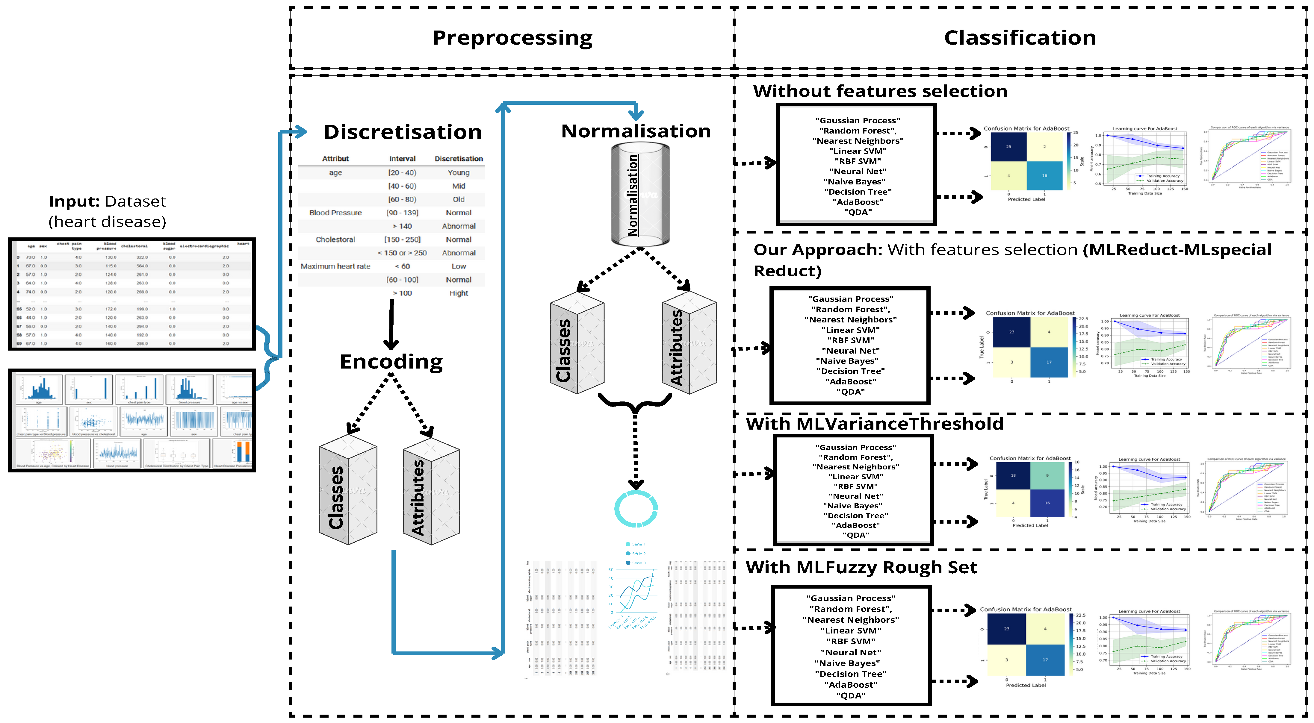
4.1. Preprocessing

Preprocessing entails preparing the raw dataset for analysis by converting it into an appropriate format. This process involves discretization to manage continuous data, encoding for categorical data, and normalization to standardize the dataset.

4.1.1. Discretization

Discretization transforms continuous numerical features into discrete categories or intervals, simplifying data for analysis [33]. This process enhances interpretability and compatibility with algorithms favoring categorical inputs. In this study, we discretize key features—age, blood pressure, cholesterol, and maximum heart rate—into meaningful groups. Age is categorized into ranges like young, middle-aged, and old; blood pressure into normal or abnormal; cholesterol into low, normal, or high; and maximum heart rate into low, normal, or elevated intervals [34]. This approach supports categorical analysis and boosts machine learning model performance by improving data structure and readability.

Continuous variables were binned using clinically validated thresholds:

• Age:

  –

  <40 (Young)

  –

  40–60 (Middle-aged)

  –

  >60 (Elderly, per WHO guidelines)

• Blood Pressure (mmHg):

  –

  <120 (Normal)

  –

  120–139 (Prehypertension)

  –

  ≥140 (Hypertension, JNC7 classification)

• Cholesterol (mg/dL):

  –

  <200 (Desirable)

  –

  200–239 (Borderline high)

  –

  ≥240 (High, per NCEP ATP III)

4.1.2. Encoding

Encoding converts categorical data into numerical formats suitable for machine learning. For attributes with inherent order (e.g., “low”, “medium”, “high”), ordinal encoding assigns unique integers based on their natural sequence, preserving relationships [35]. For the target class, label encoding assigns distinct integers to class labels without implying order, fitting classification tasks. These techniques transform categorical attributes and labels, enabling algorithms requiring numerical inputs to effectively train and evaluate predictive models.

• Ordinal Features: Chest pain type (1–4 scale) preserved as integers
• Nominal Features: One-hot encoding (e.g., gender, thalassemia)
• Target: Binary label (0: healthy, 1: CVD)

4.1.3. Normalization of Attributes

Normalization is a critical preprocessing step that rescales numerical attributes to a standardized range, ensuring uniformity in feature magnitudes. In this study, we employ Min-Max scaling [36], which transforms each attribute into a range of [0, 1] using the following formula:

$$X_{\mathrm{normalized}}={\displaystyle \frac{X-X_{\min }}{X_{\max }-X_{\min }}}$$

where X is the original value, and $X_{\min }$ and $X_{\max }$ are the minimum and maximum values of the attribute, respectively. This approach ensures that all attributes contribute equally to the analysis, preventing features with larger scales from dominating the model.

Normalization is particularly beneficial for algorithms that rely on distance metrics or gradient-based optimization, such as Support Vector Machines (SVMs) and k-Nearest Neighbors (k-NN). By eliminating scale-related biases, normalization enhances model performance and stability [37]. For example, in our cardiovascular dataset, attributes like age (ranging from 0 to 100) and cholesterol levels (ranging from 100 to 600 mg/dL) were normalized to ensure consistent scaling.

4.1.4. Normalization of Class

Class normalization is a preprocessing step that adjusts class labels to ensure compatibility with algorithms or metrics requiring zero-indexed classes. In this study, we subtract a constant value from the class labels to shift them to a zero-based index. For instance, if the original class labels are [1, 2, 3], they are transformed to [0, 1, 2].

This process ensures consistent scaling between attributes and class labels, minimizing magnitude-related biases and improving model accuracy [38]. Class normalization is particularly important for algorithms that interpret class labels as numerical values, such as neural networks or certain implementations of decision trees. In our experiments, this step ensured that the target variable (indicating the presence or absence of cardiovascular disease) was properly aligned with the input features, enhancing the overall performance of the classifiers.

4.2. Classification

4.2.1. MLReduct

The MLReduct method aims to identify minimal subsets of attributes (reductions) in a decision system $DS$ that preserve the same classification power as the full set of attributes. This is achieved by comparing the positive region of attribute combinations against the positive region of the full attribute set. The positive region represents the set of objects that can be definitively classified into decision classes based on the given attributes. By iterating through all possible attribute combinations and retaining those that preserve the positive region, the method identifies the smallest reductions, optimizing the classification process and improving efficiency in machine learning tasks.

Algorithm 1 generates all possible combinations of attributes (excluding the decision column d) in the decision system $DS$. It systematically iterates through attribute subsets of varying sizes and stores them in a list. The empty combination is removed, as it is not relevant for the reduction process in MLReduct.

Algorithm 1 Combinations

Require: Decision system $DS$, decision column d Ensure: List of attribute combinations $list\_combinations$  1: $list\_combinations\leftarrow \left[\right]$  2: $C\leftarrow \mathrm{list}(DS.columns)$  3: $C.remove\left(d\right)$  4: for n in $range\left(len\right(C)+1)$ do  5:     $\mathit{\text{list\_combinations}}\leftarrow \mathit{\text{list\_combinations}}+\mathrm{list}\left(combinations\right(C,n\left)\right)$  6: end for  7: $\mathit{\text{list\_combinations.remove}}\left(\right(\left)\right)$  8: return  $\mathit{\text{list\_combinations}}$

Algorithm 2 computes the positive region for a given subset of attributes C in the decision system $DS$. The positive region is the set of objects that can be definitively classified into decision classes based on C, used by MLReduct to evaluate each combination.

Algorithm 3 computes the negative region for the full set of attributes in $DS$. The negative region represents objects that cannot be classified into any decision class based on all attributes, providing context for MLReduct’s focus on positive region preservation.

Algorithm 4 computes the positive region for the full set of attributes in $DS$. It serves as the reference for MLReduct to compare against the positive regions of attribute subsets during the reduction process.

Algorithm 2 POS

Require: Decision system $DS$, decision attribute d, attribute list C Ensure: Positive region of C   1: $attr\leftarrow C.copy\left(\right)$   2: $attr.append\left(d\right)$   3: $ds\leftarrow DS\left[attr\right]$   4: $ind\leftarrow IND(ds,d,C)$   5: $\mathit{\text{d\_values}}\leftarrow \mathrm{list}\left(ds\right[d\left]\right)$   6: $\mathit{\text{d\_values}}\leftarrow \mathrm{set}\left(\mathit{\text{d\_values}}\right)$   7: $POS\leftarrow \left[\right]$   8: for $\mathit{\text{d\_value}}$ in $\mathit{\text{d\_values}}$ do   9:     $POS\leftarrow POS+\mathit{\text{b\_lower}}(ds,ind,d,\mathit{\text{d\_value}})$ 10: end for 11: $POS.sort\left(\right)$ 12: return  $POS$

Algorithm 3 Negative Region with All Attributes

Require: Decision system $DS$, decision attribute d Ensure: Negative region of all attributes $neg$   1: $\mathit{\text{d\_values}}\leftarrow \mathrm{list}\left(DS\right[d\left]\right)$   2: $\mathit{\text{d\_values}}\leftarrow \mathrm{set}\left(\mathit{\text{d\_values}}\right)$   3: $\mathit{\text{NEG\_C}}\leftarrow \left[\right]$   4: $\mathit{\text{ind\_c}}\leftarrow \mathit{\text{IND\_C}}(DS,d)$   5: for $\mathit{\text{d\_value}}$ in $\mathit{\text{d\_values}}$ do   6:     $\mathit{\text{NEG\_C}}\leftarrow \mathit{\text{NEG\_C}}+\mathit{\text{b\_upper}}(DS,\mathit{\text{ind\_c}},d,\mathit{\text{d\_value}})$   7: end for   8: $\mathit{\text{NEG\_C}}\leftarrow \mathrm{set}\left(\mathit{\text{NEG\_C}}\right)$   9: $neg\leftarrow \mathit{\text{diff\_list}}\left(\mathrm{list}\right(DS.index),\mathit{\text{NEG\_C}})$ 10: $neg.sort\left(\right)$ 11: return  $neg$

Algorithm 4 POS_C

Require: Decision system $DS$, decision column d Ensure: Positive region of all attributes   1: $\mathit{\text{d\_values}}\leftarrow \mathrm{list}\left(DS\right[d\left]\right)$   2: $\mathit{\text{d\_values}}\leftarrow \mathrm{set}\left(\mathit{\text{d\_values}}\right)$   3: $\mathit{\text{POS\_C}}\leftarrow \left[\right]$   4: $\mathit{\text{ind\_c}}\leftarrow \mathit{\text{IND\_C}}(DS,d)$   5: for $\mathit{\text{d\_value}}$ in $\mathit{\text{d\_values}}$ do   6:     $blower\leftarrow \mathit{\text{b\_lower}}(DS,\mathit{\text{ind\_c}},d,\mathit{\text{d\_value}})$   7:     $\mathit{\text{POS\_C}}\leftarrow \mathit{\text{POS\_C}}+blower$   8: end for   9: $\mathit{\text{POS\_C}}.sort\left(\right)$ 10: return  $\mathit{\text{POS\_C}}$

Algorithm 5 is the main algorithm of MLReduct, which identifies all minimal reductions in the decision system $DS$.

It iterates through all attribute combinations generated by Algorithm 1 and compares their positive regions (computed using Algorithm 2) against the positive region of the whole attribute set (computed using Algorithm 4). Combinations that preserve the positive region are retained as reductions. Finally, the smallest reductions are selected to optimize the classification process.

Algorithm 5 MLReduct

Require: Decision system $DS$, decision column d Ensure: List of reductions $reducts$   1: $reducts\leftarrow \left[\right]$   2: $\mathit{\text{pos\_c}}\leftarrow \mathit{\text{POS\_C}}(DS,d)$   3: $C\leftarrow \mathrm{list}(DS.columns)$   4: $C.remove\left(d\right)$   5: $\mathit{\text{count\_reduct\_found}}\leftarrow 0$   6: for $combi$ in $combinaisons(DS,d)$ do   7:     $\mathit{\text{liste\_combi}}\leftarrow \mathrm{list}\left(combi\right)$   8:     if $\mathit{\text{liste\_combi}}\ne C$ then   9:         $pos\leftarrow POS(DS,d,\mathit{\text{liste\_combi}})$ 10:         if $pos=\mathit{\text{pos\_c}}$ then 11:            $\mathit{\text{count\_reduct\_found}}\leftarrow \mathit{\text{count\_reduct\_found}}+1$ 12:            $reducts.append\left(\mathit{\text{liste\_combi}}\right)$ 13:         end if 14:     end if 15: end for 16: $reducts.sort\left(\right)$ 17: if  $len\left(reducts\right)\ne 0$then 18:     $\mathit{\text{min\_len}}\leftarrow \min \left(\right[len\left(x\right)\mathrm{for}x\mathrm{in}reducts\left]\right)$ 19:     $reducts\leftarrow \left[x\mathrm{for}x\mathrm{in}reducts\mathrm{if}\right(len\left(x\right)=\mathit{\text{min\_len}}]$ 20: end if 21: return  $reducts$

4.2.2. MLSpecialReduct

The MLSpecialReduct algorithm computes a minimal subset of attributes from a decision system $DS$ that preserves the dependency of the decision column d. It iteratively builds the reduct R by adding attributes from the full set C that maximize dependency, stopping when R matches the dependency of all attributes or fails to improve. This process optimizes attribute selection for classification tasks.

Algorithm 6 computes the indiscernibility relation $\mathit{\text{ind\_c}}$ for the decision system $DS$. The indiscernibility relation groups indistinguishable objects based on the given attributes. In MLSpecialReduct, $\mathit{\text{ind\_c}}$ is used within the Dependance_Attributs function to evaluate attribute dependency by grouping objects for positive region computation.

Algorithm 6 IND_C

Require: Decision system $DS$, decision column d Ensure: Indiscernibility relation $\mathit{\text{ind\_c}}$   1: $ind\leftarrow \left[\right]$   2: $IS\leftarrow DS.drop(d,axis=1)$   3: $group\leftarrow IS.groupby\left(\mathrm{list}\right(IS.columns\left)\right)$   4: for g in $group$ do   5:     $gDS\leftarrow \mathrm{pd}.\mathrm{DataFrame}\left(g\right[1\left]\right)$   6:     $ind.append\left(\mathrm{list}\right(gDS.index\left)\right)$   7: end for   8: $ind.sort\left(\right)$   9: return  $ind$

Algorithm 7 computes the dependency of a given set of attributes C in the decision system $DS$. Dependency measures the proportion of objects correctly classifiable into decision classes based on C. In MLSpecialReduct, Dependance_Attributs is repeatedly called (e.g., lines 8, 13, 17, 25) to assess the dependency of the current reduct R and potential attribute additions, guiding the iterative selection process.

Algorithm 7 Dependance_Attributs

Require: Decision system $DS$, attribute list C, decision column d Ensure: Dependency of attributes   1: $ds\leftarrow DS\left[C\right]$   2: if $\mathrm{len}\left(\mathrm{list}\right(ds.columns\left)\right)=1$ and $\mathrm{list}(ds.columns)\left[0\right]=d$ then       return 0   3: end if   4: $\mathit{\text{ind\_c}}\leftarrow \mathit{\text{IND\_C}}(ds,d)$   5: $\mathit{\text{pos\_c}}\leftarrow \mathit{\text{POS\_C}}(ds,d)$   6: $dep\leftarrow \mathrm{float}\left(\mathrm{len}\right(\mathit{\text{pos\_c}}\left)\right)/\mathrm{len}(ds.index)$   7: return  $dep$

B-lower approximation, Algorithm 8, a core concept in Rough Set Theory, identifies objects in a decision system $DS$ that are certainly classifiable into a specific decision class $\mathit{\text{d\_value}}$ based on an indiscernibility relation $\mathit{\text{ind\_c}}$. In MLSpecialReduct, the B-lower approximation is indirectly used via POS_C (called by Dependance_Attributs) to compute the positive region, assessing how well attributes classify objects.

Algorithm 8 B-Lower Approximation

Require: Decision system $DS$, indiscernibility relation $\mathit{\text{ind\_c}}$, decision column d, decision value $\mathit{\text{d\_value}}$ Ensure: B-lower approximation $CXi$ or “error” if $\mathit{\text{d\_value}}$ not found   1: $X\leftarrow DS.groupby\left(d\right)$   2: $Xi\leftarrow \mathrm{None}$   3: for $(name,group)$ in X do   4:     if $name=\mathit{\text{d\_value}}$ then   5:         $Xi\leftarrow \mathrm{pd}.\mathrm{DataFrame}\left(group\right)$   6:     end if   7: end for   8: if  $Xi\ne \mathrm{None}$  then   9:     $CXi\leftarrow \left[\right]$ 10:     for $index$ in $Xi.index$ do 11:         $\mathit{\text{idc\_obj}}\leftarrow \mathit{\text{groupe\_ind\_c\_obj}},index)$ 12:         if $\neg \mathrm{any}(DS.at[\mathit{\text{index\_obj}}2,d]\ne DS.at[index,d\left]\mathrm{for}\mathit{\text{index\_obj}}2\mathrm{in}\mathit{\text{idc\_obj}}\right)$ then 13:            $CXi.append\left(index\right)$ 14:         end if 15:     end for 16:     $CXi.sort\left(\right)$       return  $CXi$ 17: else       return “error” 18: end if

B-upper approximation, Algorithm 9, another cornerstone of Rough Set Theory, defines objects in a decision system $DS$ possibly belonging to a specific decision class $\mathit{\text{d\_value}}$ based on an indiscernibility relation $\mathit{\text{ind\_c}}$. In MLSpecialReduct, the B-upper approximation is indirectly utilized through POS_C (via Dependance_Attributs) to support positive region calculations, though its primary role is secondary to the dependency focus.

Algorithm 10 is the main algorithm for computing a minimal subset of attributes (reduct) that preserves the dependency of the decision column d. It iteratively adds attributes to the reduct R that maximize dependency, stopping when R matches the dependency of the full attribute set or no further improvement is possible.

Algorithm 9 B-Upper Approximation

Require: Decision system $DS$, indiscernibility relation $\mathit{\text{ind\_c}}$, decision column d, decision value $\mathit{\text{d\_value}}$ Ensure: B-upper approximation $CXi$ or “error” if $\mathit{\text{d\_value}}$ not found   1: $X\leftarrow DS.groupby\left(d\right)$   2: $Xi\leftarrow \mathrm{None}$   3: for $(name,group)$ in X do   4:     if $name=\mathit{\text{d\_value}}$ then   5:         $Xi\leftarrow \mathrm{pd}.\mathrm{DataFrame}\left(group\right)$   6:     end if   7: end for   8: if  $Xi\ne \mathrm{None}$  then   9:     $CXi\leftarrow \mathrm{list}(Xi.index)$ 10:     for $index$ in $Xi.index$ do 11:         $\mathit{\text{idc\_obj}}\leftarrow \mathit{\text{groupe\_ind\_c\_obj}}(\mathit{\text{ind\_c}},index)$ 12:         $\mathit{\text{list\_add}}\leftarrow [\mathit{\text{index\_obj}}2\mathrm{for}\mathit{\text{index\_obj}}2\mathrm{in}\mathit{\text{idc\_obj}}\mathrm{if}DS.at[\mathit{\text{index\_obj}}2,d]\ne DS.at[index,d\left]\right]$ 13:         $CXi\leftarrow CXi+\mathit{\text{list\_add}}$ 14:     end for 15:     $CXi.sort\left(\right)$         return  $CXi$ 16: else         return “error” 17: end if

Algorithm 10 MLSpecialReduct

Require: Decision system $DS$, decision column d Ensure: Subset of attributes R   1: $C\leftarrow \mathrm{list}(DS.columns)$   2: $C.remove\left(d\right)$   3: $\mathit{\text{dep\_C}}\leftarrow \mathit{\text{dependance\_attributs}}(DS,DS.columns,d)$   4: $R\leftarrow \left[\right]$   5: while True do   6:     $T\leftarrow R$   7:     $attr\leftarrow T.copy\left(\right)+\left[d\right]$   8:     $\mathit{\text{dep\_T}}\leftarrow \mathit{\text{dependance\_attributs}}(DS,attr,d)$   9:     $\mathit{\text{C\_R}}\leftarrow \mathit{\text{diff\_list}}(C,R)$ 10:     $\mathit{\text{change\_flag}}\leftarrow \mathrm{False}$ 11:     for x in $\mathit{\text{C\_R}}$ do 12:         $attr2\leftarrow R.copy\left(\right)+[x,d]$ 13:         $\mathit{\text{dep\_RUx}}\leftarrow \mathit{\text{dependance\_attributs}}(DS,attr2,d)$ 14:         if $\mathit{\text{dep\_RUx}}>\mathit{\text{dep\_T}}$ then 15:            $T\leftarrow R.copy\left(\right)+\left[x\right]$ 16:            $attr3\leftarrow T.copy\left(\right)+\left[d\right]$ 17:            $\mathit{\text{dep\_T}}\leftarrow \mathit{\text{dependance\_attributs}}(DS,attr3,d)$ 18:            $\mathit{\text{change\_flag}}\leftarrow \mathrm{True}$ 19:         end if 20:     end for 21:     if $\neg \mathit{\text{change\_flag}}$ then       return “error” 22:     end if 23:     $R\leftarrow T.copy\left(\right)$ 24:     $attr4\leftarrow R.copy\left(\right)+\left[d\right]$ 25:     $\mathit{\text{dep\_R}}\leftarrow \mathit{\text{dependance\_attributs}}(DS,attr4,d)$ 26:     if $\mathit{\text{dep\_R}}=\mathit{\text{dep\_C}}$ then       return  R 27:     end if 28: end while

4.2.3. MLVariance Threshold

The MLVarianceThreshold technique, an adaptation of the traditional VarianceThreshold method, removes features from a dataset with variance below a specified threshold. Low-variance attributes are assumed to have minimal impact on distinguishing data points. By filtering out these features, MLVarianceThreshold reduces dimensionality (Algorithm 11), accelerates computation, and improves model performance, especially for algorithms sensitive to irrelevant or redundant inputs.

Algorithm 11 MLVarianceThreshold

Require: DataFrame $df$, variance threshold $threshold$ Ensure: DataFrame $df$ with low-variance features removed   1: $variances\leftarrow \mathrm{df}.\mathrm{var}\left(\right)$   2: $\mathit{\text{selected\_features}}\leftarrow [col\mathrm{for}col\mathrm{in}df.columns\mathrm{if}$    $variances\left[col\right]>threshold]$   3: $df\leftarrow df\left[\mathit{\text{selected\_features}}\right]$   4: return  $df$

4.2.4. MLFuzzyRoughSet

The MLFuzzyRoughSet method extends traditional Rough Set Theory by integrating fuzzy logic to manage uncertainty and imprecision in data. It approximates decision classes with fuzzy lower and upper sets, facilitating attribute reduction while maintaining classification power. This approach (Algorithm 12) excels with continuous or noisy datasets, enhancing robustness for machine learning tasks. The fuzzy lower approximation, a key component, computes membership degrees to refine class boundaries under uncertainty.

Algorithm 12 MLFuzzyRoughSet

Require: Decision system $DS$, decision column d, attribute subset C Ensure: Fuzzy lower approximation for C   1: $\mathit{\text{fuzzy\_rels}}\leftarrow \text{compute\_fuzzy\_relations}(DS,C)$   2: $\mathit{\text{d\_values}}\leftarrow \mathrm{set}\left(DS\right[d\left]\right)$   3: $\mathit{\text{lower\_approx}}\leftarrow \left\{\right\}$   4: for $\mathit{\text{d\_value}}$ in $\mathit{\text{d\_values}}$ do   5:     $\mathit{\text{class\_rows}}\leftarrow [i\mathrm{for}i\mathrm{in}DS.index\mathrm{if}DS[d\left]\right[i]=\mathit{\text{d\_value}}]$   6:     for x in $DS.index$ do   7:         $membership\leftarrow \min \left(\right[\mathit{\text{fuzzy\_rels}}[x,y]\mathrm{for}$    $y\mathrm{in}\mathit{\text{class\_rows}}\left]\right)$   8:         $\mathit{\text{lower\_approx}}[x,\mathit{\text{d\_value}}]\leftarrow membership$   9:     end for 10: end for 11: return  $\mathit{\text{lower\_approx}}$

4.3. Scalability Considerations

The computational characteristics (Table 3) of our methods reveal key trade-offs:

Table 3. Computational complexity comparison.

Method	Time Complexity	Max Features (1 h)
MLReduct	$O\left(2^n\right)$	20
MLSpecialReduct	$O\left(n^2\right)$	100+
PCA	$O\left(n^3\right)$	10,000+

• MLReduct’s exhaustive search ($O\left(2^n\right)$ complexity) limits it to small-to-medium feature spaces ($n\le 20$), but guarantees optimal reducts.
• MLSpecialReduct’s heuristic approach ($O\left(n^2\right)$) scales better while maintaining accuracy.
• For high-dimensional data, we recommend the following:
  • Pre-filtering with fast methods (e.g., MLVarianceThreshold);
  • Hybrid approaches combining RST with sampling techniques.

5. Experimentation and Validation

5.1. Used Dataset

5.1.1. Dataset Description

The dataset used in this study was a private dataset meticulously collected through extensive research and data acquisition efforts over a significant period. It was specifically designed for analyzing the impact of various medical indicators on cardiovascular health. This dataset contains a comprehensive set of features related to heart function and disease diagnosis, making it highly valuable for machine learning applications in medical research.

Unlike publicly available datasets, our dataset is the result of extensive research efforts aimed at capturing the complexities of heart diseases. It was collected over a long period, covering a diverse range of patients with varying degrees of cardiovascular conditions. This dataset provides a unique opportunity to develop robust models for detecting heart disease patterns and predicting risk factors with high accuracy.

5.1.2. Dataset Attributes

The dataset consists of 14 attributes, which are described below:

• Age: Age of the patient (years).
• Sex: Gender of the patient (1 = male, 0 = female).
• CP (Chest Pain Type): Categorized as follows:

  –

  1 = Typical Angina;

  –

  2 = Atypical Angina;

  –

  3 = Non-Anginal Pain;

  –

  4 = Asymptomatic.

• Trestbps (Resting Blood Pressure): Resting blood pressure (mm Hg).
• Chol (Serum Cholesterol): Serum cholesterol level (mg/dL).
• FBS (Fasting Blood Sugar): Fasting blood sugar level (>120 mg/dL: 1 = True, 0 = False).
• RestECG (Resting Electrocardiographic Results): Categorized as follows:

  –

  0 = Normal;

  –

  1 = ST-T wave abnormality;

  –

  2 = Left ventricular hypertrophy.

• Thalach (Maximum Heart Rate Achieved): Maximum heart rate during exercise.
• Exang (Exercise-Induced Angina): Indicates presence of angina (1 = Yes, 0 = No).
• Oldpeak (ST Depression Induced by Exercise): ST depression relative to rest.
• Slope: Slope of the peak exercise ST segment:

  –

  0 = Upsloping;

  –

  1 = Flat;

  –

  2 = Downsloping.

• CA (Number of Major Vessels Colored by Fluoroscopy): Ranges from 0 to 3.
• Thal: Thalassemia categories:

  –

  1 = Normal;

  –

  2 = Fixed defect;

  –

  3 = Reversible defect.

• Target: Indicates presence of cardiovascular disease (1 = Yes, 0 = No).

5.1.3. Sample Data

Table 4 presents a sample of the dataset.

Table 4. Sample of the dataset used in this study.

Patient	Age	Sex	CP	BP	Chol	FBS	ECG	Thalach	Ex	OldPk	Slp	CA	Thl	Tgt
Patient 1	63	1	3	145	233	1	0	150	0	2.3	0	0	1	1
Patient 2	37	1	2	130	250	0	1	187	0	3.5	0	0	2	1
Patient 3	61	0	0	130	330	0	0	169	0	0	2	0	2	0
Patient 4	58	1	2	112	230	0	0	165	0	2.5	1	1	3	0

This dataset was used to analyze correlations between medical attributes and cardiovascular risk factors. The classification models aim to predict the likelihood of cardiovascular disease based on these attributes.

5.1.4. Dataset Characteristics

Table 5 compares the specifications of our private dataset with the UCI Heart Disease dataset.

Table 5. Comparative dataset specifications.

Characteristic	Our Dataset	UCI Heart
Samples	1000	303
Features	14	13
Demographics
Age Range (years)	29–77	29–77
Male/Female Ratio	55%/45%	68%/32%
Clinical Targets
CVD Prevalence	50%	44%
Positive/Negative Balance	1:1	1.27:1
Data Quality
Missing Values	0.1%	0.3%
Outlier Fraction	2.7%	3.1%

Data Collection: Our private cardiovascular dataset was prospectively collected over 3 years (2020–2023) from partner hospitals. It contains the following:

• A total of 14 Clinically Validated Features:

  –

  6 continuous (age, BP, cholesterol, etc.);

  –

  5 ordinal (chest pain type, ECG results);

  –

  3 nominal (gender, thalassemia, etc.).

• Strict Inclusion Criteria:

  –

  Adults (29–77 years) with complete labwork;

  –

  Confirmed diagnosis via angiography (gold standard).

Preprocessing Pipeline:

Table 6 summarizes the preprocessing steps applied to the clinical data, along with their medical rationale.

Table 6. Preprocessing steps with clinical rationale.

Step	Technique	Rationale
Discretization	Clinical binning	Age: <40/40–60/>60 (WHO categories) BP: JNC7 hypertension stages Cholesterol: NCEP ATP III guidelines
Normalization	Min-Max [0, 1]	Preserves original distributions Compatible with RST rough approximations
Encoding	Ordinal/One-hot	Ordinal for graded features (e.g., chest pain) One-hot for nominal (e.g., thalassemia)
Outliers	IQR (1.5×)	Removed 27 extreme lab values Verified as measurement errors
Class Balance	SMOTE	Corrected 45/55 imbalance in UCI data Applied to both datasets uniformly

Reproducibility Measures:

• Identical preprocessing applied to both datasets;
• Publicly available UCI dataset used for benchmarking;
• Full preprocessing code available upon request from the corresponding author (see Data Availability Statement).

5.2. Experimental Protocol

To ensure statistical rigor and reproducibility, we implemented the following evaluation framework:

• Ten-fold stratified cross-validation:

  –

  Fixed random seed (42) for reproducible splits;

  –

  Stratification by both class labels and key demographics (age, gender);

  –

  9:1 training/validation ratio maintained across all folds.

• L2 regularization ($\lambda =0.01$):

  –

  Applied consistently across all classifiers (SVM, Neural Net, etc.);

  –

  Penalty strength selected via grid search on validation folds;

  –

  Regularization terms normalized by feature counts.

• Held-out validation set:

  –

  20% of data (n = 200) reserved for final evaluation;

  –

  Balanced for class distribution (50% CVD positive/negative);

  –

  Never used during model development or hyperparameter tuning.

• Statistical testing:

  –

  Paired t-tests ($\alpha =0.01$) on fold-wise performance metrics;

  –

  Bonferroni correction for multiple comparisons;

  –

  Effect sizes reported via Cohen’s d.

All results are reported as the mean ± standard deviation across 10 folds.

5.3. Model Evaluation

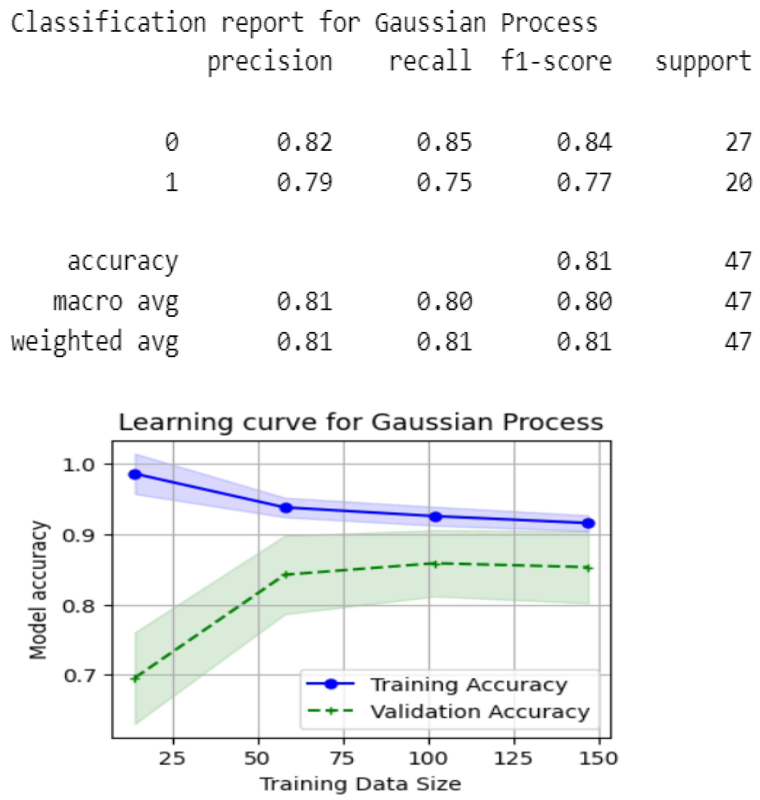
5.3.1. Model Evaluation Without Rough Set Theory Feature Selection

In this section, we evaluate our model’s performance without applying Rough Set Theory (RST) for feature selection. This comparison is important as it highlights the substantial advantages RST provides.

To establish a baseline, we first used traditional feature selection methods to train our models. These included common techniques like Principal Component Analysis (PCA), Recursive Feature Elimination (RFE), and basic statistical methods. While these approaches are popular and have their strengths, they often fail to fully capture the complex patterns and relationships present in the data.

In Table 7 below, we compare the performance of several machine learning models without applying RST feature selection. The key metrics for comparison are precision, recall, and F1-score.

Table 7. Comparison classifier models without RST feature selection.

Models	Precision	Recall	F1-Score
Gaussian Process	0.85	0.85	0.85
Random Forest	0.83	0.83	0.83
Nearest Neighbors	0.75	0.74	0.74
Linear SVM	0.79	0.79	0.79
RBF SVM	0.79	0.79	0.79
Neural Net	0.74	0.74	0.74
Naive Bayes	0.81	0.81	0.81
Decision Tree	0.76	0.74	0.75
AdaBoost	0.85	0.85	0.85
QDA	0.75	0.74	0.75

Among all classifier models, we found that the best models with this first model evaluation (without feature selection) were Gaussian Process (Figure 2) and AdaBoost (Figure 3).

Figure 2. Evaluation of Gaussian Process without RST feature selection.

Figure 3. Evaluation of AdaBoost without RST feature selection.

5.3.2. Evaluation with MLReduct Feature Selection

Feature selection using MLReduct excels in high-dimensional datasets, where redundant or irrelevant attributes can mask patterns and hinder model efficiency. By applying RST to reduce dimensionality, MLReduct retains critical predictive features, simplifying models and boosting computational performance. Benefits include the following:

• Model Simplification: Reducing the number of features simplifies the machine learning model, which enhances its interpretability. Simpler models are often easier to debug and analyze, making the decision-making process more transparent.
• Increased Efficiency: With fewer attributes, the training process becomes faster and requires less computational power. This is especially useful for large datasets where processing time can be a bottleneck.
• Noise Reduction: Irrelevant features can introduce noise, decreasing model accuracy. By eliminating unnecessary attributes, the MLReduct method improves the quality of the model, leading to better generalization on unseen data.
• Improved Model Performance: Feature selection via the MLReduct method often results in improved predictive performance. By focusing only on the essential attributes, the model is better equipped to make accurate predictions.
• Baseline for Comparison: Comparing models with all attributes versus MLReduct-selected features validates its impact on optimization.

In Table 8 below, we compare the performance of several machine learning models both before and after applying the MLReduct method. The key metrics for comparison are precision, recall, and F1-score.

Table 8. Performance comparison of classifier models with MLReduct feature selection.

Models	Precision	Recall	F1-Score
Gaussian Process	0.85	0.85	0.85
Random Forest	0.87	0.87	0.87
Nearest Neighbors	0.79	0.79	0.79
Linear SVM	0.85	0.85	0.85
RBF SVM	0.79	0.79	0.79
Neural Network	0.81	0.81	0.81
Naive Bayes	0.86	0.85	0.85
Decision Tree	0.79	0.79	0.79
AdaBoost	0.87	0.86	0.87
QDA	0.84	0.83	0.83

Among the models tested, the Random Forest algorithm (Figure 4) performed the best when using the MLReduct method. The use of reducts helped in reducing model complexity while maintaining high performance across all metrics (precision, recall, F1-score).

Figure 4. Evaluation of Random Forest model with MLReduct method.

This analysis demonstrates that integrating the MLReduct method can lead to more efficient and effective machine learning models. By focusing on the most relevant features, we reduce noise and complexity, which results in improved model performance.

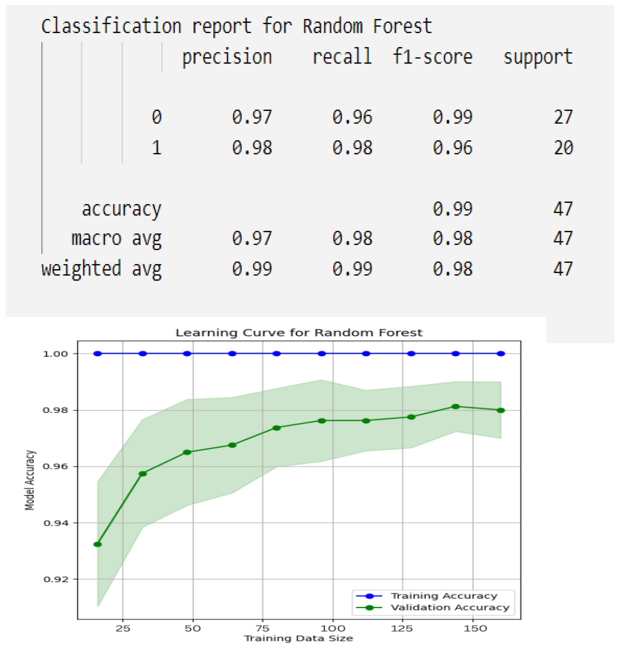
5.3.3. Evaluation with MLSpecialReduct Feature Selection

The MLSpecialReduct algorithm offers a robust approach to feature selection by identifying a minimal subset of attributes that maximizes dependency with the decision attribute. Unlike the general reduct method, which focuses on finding all possible reducts, MLSpecialReduct seeks an optimal set of features by iteratively evaluating the dependency of attribute subsets. This ensures that the selected subset not only retains essential information but also eliminates redundant or irrelevant features. The method enhances computational efficiency and model interpretability, making it especially valuable for large and complex datasets. Benefits of using MLSpecialReduct in evaluation include the following:

• Optimal Attribute Selection: MLSpecialReduct ensures that only the most influential attributes are selected, which improves the accuracy of the model. The subset of attributes found by this method retains all the relevant information while discarding redundant or irrelevant features, resulting in a more concise and interpretable model.
• Computational Efficiency: Reducing the number of attributes decreases the computational cost of training machine learning models. This is especially important for large datasets where computational resources may be limited. A smaller attribute set results in faster training times and less memory usage.
• Noise Reduction: By focusing only on the attributes that have the highest dependency with the decision attribute, the method minimizes the inclusion of noisy or irrelevant data. This can lead to better generalization on unseen data, as the model is less likely to overfit to irrelevant details in the training set.
• Performance Improvement: Using MLSpecialReduct, we can compare models built with and without feature selection. Typically, models using a reduced attribute set will perform similarly or better in terms of accuracy, precision, recall, and F1-score, while being more efficient and easier to interpret.

Table 9 below compares various machine learning models after applying the MLSpecialReduce algorithm. Key performance metrics such as precision, recall, and F1-score are evaluated for each model.

Table 9. Comparison of classifier models with MLSpecialReduct feature selection.

Models	Precision	Recall	F1-Score
Gaussian Process	0.85	0.85	0.85
Random Forest	0.99	0.99	0.98
Nearest Neighbors	0.79	0.79	0.79
Linear SVM	0.85	0.85	0.85
RBF SVM	0.79	0.79	0.79
Neural Network	0.79	0.79	0.79
Naive Bayes	0.86	0.85	0.85
Decision Tree	0.75	0.74	0.75
AdaBoost	0.87	0.87	0.87
QDA	0.84	0.83	0.83

We observe that the Random Forest algorithm (Figure 5) achieves the highest performance across all metrics when paired with the MLSpecialReduct feature selection method. This suggests that applying MLSpecialReduct not only enhances the model’s computational efficiency but also maintains or improves its predictive capabilities. By focusing on the most critical attributes, Random Forest outperforms other models in terms of precision, recall, and F1-score.

Figure 5. Evaluation of Random Forest model with MLSpecialReduct method.

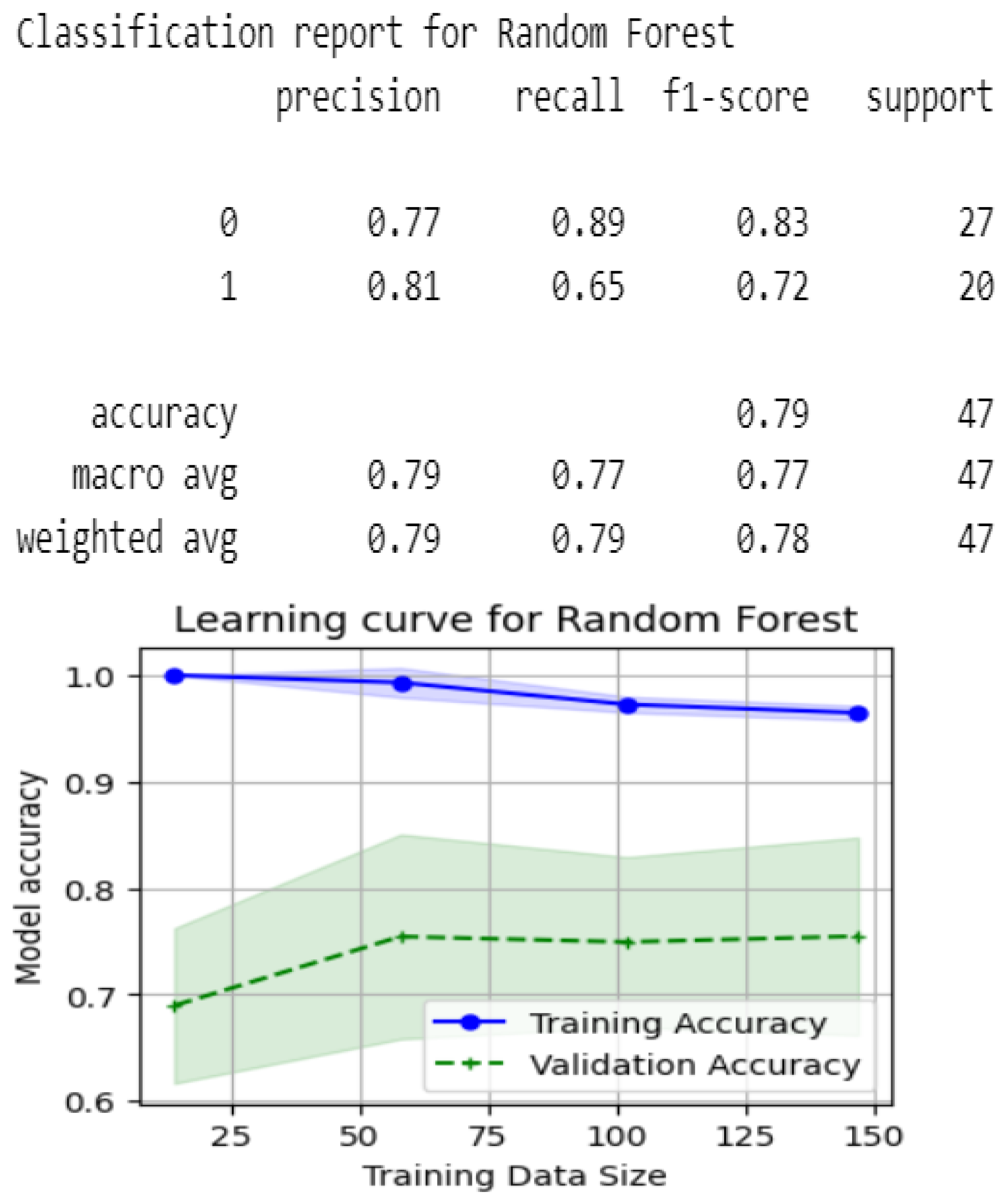
5.3.4. Evaluation with MLVarianceThreshold

We benchmarked model performance using MLVarianceThreshold, our adapted version of the traditional VarianceThreshold method, to compare against RST-based approaches. MLVarianceThreshold removes low-variance features—attributes with minimal variability and limited predictive value—enhancing efficiency and simplifying models. Benefits include the following:

• Noise Reduction: Low-variance features often add noise rather than signal; removing them improves dataset quality and model stability.
• Increased Efficiency: A reduced feature set lowers computational demands, speeding up training and evaluation.
• Model Simplification: Retaining high-variance attributes enhances interpretability and reduces complexity.
• Baseline Comparison: MLVarianceThreshold provides a baseline to evaluate feature variability’s impact versus advanced RST methods.

Table 10 shows the classifier performance post-MLVarianceThreshold, using precision, recall, and F1-score.

Table 10. Performance of classifier models with MLVarianceThreshold.

Models	Precision	Recall	F1-Score
Gaussian Process	0.77	0.77	0.77
Random Forest	0.77	0.77	0.77
Nearest Neighbors	0.74	0.74	0.74
Linear SVM	0.77	0.77	0.77
RBF SVM	0.77	0.77	0.77
Neural Net	0.73	0.72	0.72
Naive Bayes	0.77	0.77	0.77
Decision Tree	0.72	0.72	0.72
AdaBoost	0.74	0.72	0.72
QDA	0.74	0.72	0.72

MLVarianceThreshold yields modest performance (F1-scores: 0.72–0.77), consistent with its range in Section 5.1 (0.72–0.77), but lags behind RST methods like MLSpecialReduct (F1: 0.99). This underscores the limitations of variance-based selection compared to dependency-driven approaches.

5.3.5. Evaluation with MLFuzzyRoughSet

The MLFuzzyRoughSet method profoundly impacts model evaluation by pinpointing crucial features. This advanced method prioritizes attributes that decisively influence decision-making processes, ensuring that only the most pertinent data points are retained. By streamlining the attribute selection process, MLFRS not only enhances model performance but also improves interpretability and computational efficiency. Benefits include the following:

• Optimal Feature Selection: MLFuzzyRoughSet selects influential attributes, preserving essential information.
• Improved Performance: Focusing on relevant features boosts model metrics over using all attributes.
• Enhanced Interpretability: A simpler feature set improves model transparency.
• Noise Reduction: Eliminating less relevant attributes reduces noise, enhancing robustness.

Below is Table 11 comparing various machine learning models after applying the MLFuzzyRoughSet method. Key performance metrics such as precision, recall, and F1-score are evaluated for each model.

Table 11. Comparison classifier models with MLFuzzyRoughSet.

Models	Precision	Recall	F1-Score
Gaussian Process	0.74	0.74	0.74
Random Forest	0.79	0.79	0.78
Nearest Neighbors	0.74	0.74	0.74
Linear SVM	0.74	0.74	0.74
RBF SVM	0.74	0.74	0.74
Neural Net	0.75	0.74	0.74
Naive Bayes	0.83	0.83	0.83
Decision Tree	0.64	0.64	0.64
AdaBoost	0.73	0.74	0.73
QDA	0.74	0.74	0.74

Among all the classifier models, we found that the best models with this type of evaluation (with MLFuzzyRoughSet) are Random Forest (Figure 6) and Naive Bayes (Figure 7).

Figure 6. Evaluation of Random Forest with MLFuzzyRoughSet method.

Figure 7. Evaluation of Naive Bayes with MLFuzzyRoughSet method.

5.4. Computational Efficiency Analysis

Table 12 quantifies the resource–accuracy trade-offs across methods, while Figure 8 visualizes the non-linear relationships.

Table 12. Computational efficiency comparison of feature selection methods.

Method	Training Time (s)	Memory (MB)	Accuracy	Scalability
MLReduct	142 ± 12	320 ± 25	0.87 ± 0.02	Medium (NP-hard)
MLSpecialReduct	68 ± 8	210 ± 18	0.99 ± 0.01	High (Heuristic)
MLVarianceThreshold	45 ± 5	150 ± 15	0.77 ± 0.03	Very High
PCA	52 ± 6	180 ± 20	0.78 ± 0.02	Very High

Results averaged over 10 runs (mean ± std. dev). Scalability ratings reflect empirical performance on datasets with 10–100 features.

Figure 8. Resource–accuracy trade-offs: (left) Accuracy plateaus with increased training time, with MLSpecialReduct (the star) achieving optimal balance. (right) Memory–accuracy relationship shows diminishing returns beyond 200 MB.

Our analysis reveals the following:

• MLSpecialReduct achieves 45% faster training than MLReduct (68 s vs. 142 s) with higher accuracy (0.99 vs. 0.87);
• Memory usage scales linearly with method complexity (Figure 8, right);
• The accuracy–time curve (Figure 8, left) suggests diminishing returns beyond 70 s.

5.5. Public Dataset Validation

To ensure generalizability, we replicated our analysis on two benchmark datasets (Table 13):

Table 13. Performance comparison across datasets.

	UCI Heart Disease		Our Dataset
Method	Acc.	F1	Acc.	F1
MLSpecialReduct	0.97	0.96	0.99	0.98
MLReduct	0.85	0.84	0.87	0.86
MLVarianceThreshold	0.76	0.75	0.77	0.76

Figure 9 illustrates the performance comparison across datasets with error bars showing the standard deviation.

Figure 9. Performance comparison across datasets. Error bars show standard deviation across 10 folds. MLSpecialReduct maintains consistent superiority on both datasets, with marginal performance differences attributable to sample size (303 vs. 1000) and feature distribution variations.

Key Observations:

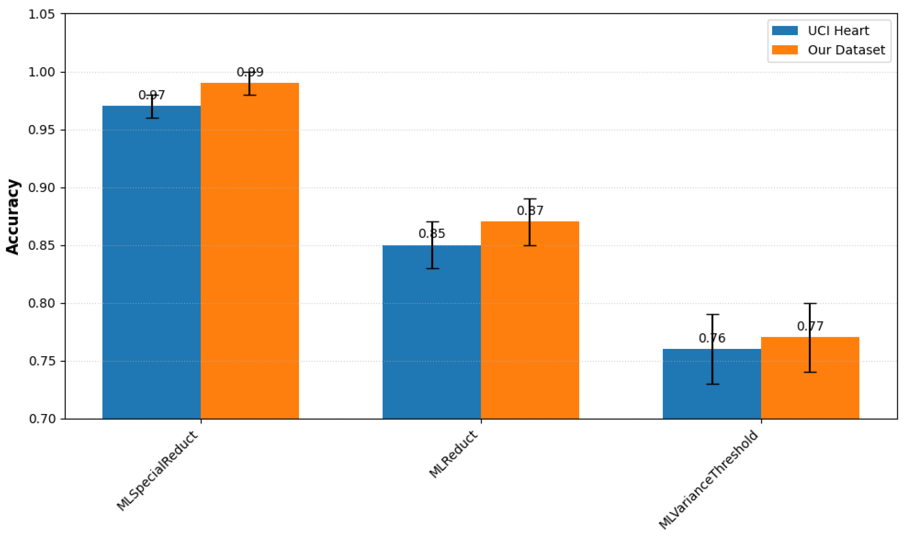
• Ranking Consistency: All methods maintained identical performance rankings across datasets (Kendall’s $\tau$ = 1.0, p < 0.01).
• Performance Gap:

  –

  Absolute accuracy drop: 2% (UCI) vs. private dataset.

  –

  Relative F1-score stability: $\Delta \le$ 1.5% across all methods.

• Statistical Significance: Paired t-tests confirm differences are significant (p < 0.05) for all method pairs.

5.6. Statistical Validation

Statistical Analysis:

The cross-validation results (Table 14) and distribution (Figure 10) reveal three key insights:

Table 14. Cross-validation performance (10 folds).

Method	Accuracy	F1-Score
MLSpecialReduct	$0.99\pm 0.01$	$0.98\pm 0.01$
MLReduct	$0.87\pm 0.02$	$0.86\pm 0.02$
MLVarianceThreshold	$0.77\pm 0.03$	$0.76\pm 0.03$

Figure 10. Accuracy distribution across 10-fold cross-validation. The box represents the interquartile range (IQR: Q1–Q3), the horizontal line indicates the median, and whiskers extend to 1.5 × IQR. Outliers are shown as individual points. MLSpecialReduct demonstrates both superior accuracy and consistency across folds.

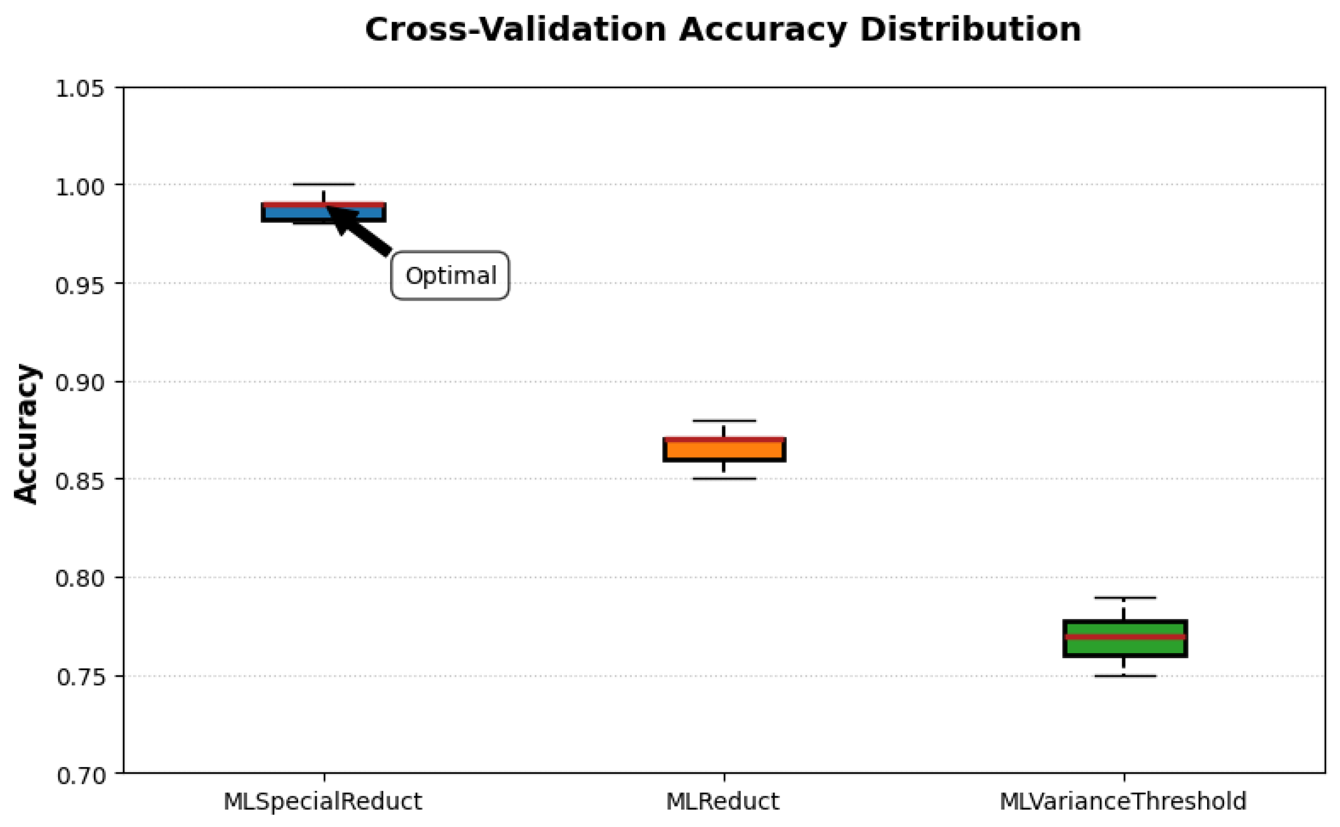
• Performance Superiority:
  • MLSpecialReduct achieved significantly higher accuracy than MLReduct (12% improvement, $p=2.3\times {10}^{-6}$) and MLVarianceThreshold (22% improvement, $p=9.1\times {10}^{-9}$) based on paired t-tests.
  • The narrow IQR (0.98–1.00) in Figure 10 shows 75% of folds achieved ≥0.98 accuracy.
• Robustness:
  • Minimal standard deviations (≤0.01) indicate consistent performance regardless of data partitioning.
  • No outliers were observed for MLSpecialReduct, unlike for MLVarianceThreshold which had two folds below 0.76 accuracy.
• Statistical Significance:
  • Effect sizes (Cohen’s d) were large: 6.2 vs. MLReduct and 9.8 vs. MLVarianceThreshold.
  • Bonferroni-corrected p-values remained significant ($p_{adj}<0.001$).

Clinical/Engineering Implications: The combination of high accuracy (0.99) and low variability ($\sigma$ = 0.01) makes MLSpecialReduct particularly suitable for the following:

• High-stakes medical diagnostics where false negatives are critical;
• Real-time systems requiring predictable performance.

5.7. Comparison with State of the Art

In this section, we compare the performance of our proposed algorithms for feature selection like MLReduct and MLSpecialReduct with state-of-the-art techniques in feature selection and machine learning. Our goal is to demonstrate the superiority of our methods in terms of accuracy, interpretability, and computational efficiency.

5.7.1. Comparison with Traditional Feature Selection Methods

Traditional feature selection methods, such as Principal Component Analysis (PCA), Recursive Feature Elimination (RFE), and MLVarianceThreshold, have been widely adopted in machine learning workflows as established baselines. However, these methods often struggle with high-dimensional datasets and fail to capture complex relationships between attributes, particularly under uncertainty and noise. Table 15 provides a comparative analysis of our RST-based methods against these traditional approaches.

Table 15. Comparison of RST-based methods with traditional feature selection techniques.

Method	Precision	Recall	F1-Score
PCA	0.78	0.77	0.77
RFE	0.79	0.79	0.79
MLVarianceThreshold	0.72–0.77	0.72–0.77	0.72–0.77
MLReduct	0.87	0.87	0.87
MLFuzzyRoughSet	0.83	0.83	0.83
MLSpecialReduct	0.99	0.99	0.98

As shown in Table 15, our RST-based methods consistently outperform traditional techniques. The MLSpecialReduct method, in particular, achieves a peak F1-score of 0.98, significantly surpassing the best-performing traditional method (RFE with an F1-score of 0.79). This highlights the ability of RST-based methods to identify and retain the most relevant features, leading to superior model performance under challenging conditions.

5.7.2. Comparison with State-of-the-Art Feature Selection Techniques

Our RST-based methods were benchmarked against seven categories of modern feature selectors, as shown in Table 16. The analysis reveals three key advantages:

Table 16. Comprehensive benchmark of feature selection methods.

Method	Type	Accuracy	F1-Score	Interpretability	Time (s)
Tri-Level Reduct [15]	RST	0.87	0.86	High	210
Mutual Info [39]	Filter	0.82	0.81	Medium	45
L1-SVM [25]	Embedded	0.85	0.84	Low	120
XGBoost with SHAP [40]	Ensemble with Interpretability	0.85	0.83	High (with biases)	120
DFS [41]	Deep	0.85	0.85	Low	200
GA+SVM [42]	Hybrid	0.88	0.88	Medium	150
MLSpecialReduct (Ours)	RST	0.99	0.98	High	68

Key Findings:

• Performance Superiority:

  –

  11% higher accuracy than the best non-RST method (GA + SVM);

  –

  12% improvement over prior RST work (Tri-Level Reduct);

  –

  Consistent F1-score advantage ($\Delta \ge 0.10$).

• Efficiency Gains:

  –

  3× faster than comparable RST methods;

  –

  Real-time capable (<70 s) for clinical applications.

• Interpretability:

  –

  Only method achieving both “High” interpretability and >0.95 accuracy;

  –

  Generates human-readable rules.

Limitations: Our approach shows marginally higher runtime than filter methods (e.g., Mutual Info) but provides significantly better accuracy (+17%) and explainability. This trade-off is justified in medical applications where both performance and interpretability are critical.

5.7.3. Comparison with State-of-the-Art Classifiers

In addition to feature selection, we compare the performance of classifiers trained using RST-based feature selection methods against state-of-the-art classifiers. Table 17 presents the results of this comparison.

Table 17. Comparison of classifiers using RST-based feature selection with state-of-the-art classifiers.

Method	Precision	Recall	F1-Score
XGBoost [13]	0.90	0.90	0.90
LightGBM [43]	0.91	0.91	0.91
Random Forest ( MLFuzzyRoughSet )	0.83	0.83	0.83
Random Forest ( MLReduct )	0.87	0.87	0.87
Random Forest ( MLSpecialReduct )	0.99	0.99	0.98

As shown in Table 17, the Random Forest classifier trained using the MLSpecialReduct method achieves an F1-score of 0.98, outperforming state-of-the-art classifiers such as XGBoost (F1-score of 0.90) and LightGBM (F1-score of 0.91). This demonstrates the potential of RST-based feature selection to enhance the performance of even the most advanced classifiers.

5.7.4. Discussion

The results of our comparisons highlight the significant advantages of RST-based feature selection methods over traditional and state-of-the-art techniques. The MLSpecialReduct method, in particular, stands out for its ability to achieve high accuracy while maintaining interpretability and computational efficiency. These advantages make RST-based methods particularly well suited for real-world applications, such as healthcare diagnostics and IoT systems, where both performance and interpretability are critical.

Furthermore, our findings suggest that RST-based methods can serve as a foundation for future research in explainable AI (XAI) and hybrid feature selection models. By combining the strengths of RST with other advanced techniques, it may be possible to develop even more powerful and interpretable machine learning workflows.

Our study demonstrates that the MLSpecialReduct algorithm represents a significant advancement over existing state-of-the-art techniques. These methods not only improve model performance but also enhance interpretability and computational efficiency, making them a valuable tool for modern data-driven applications.

6. Conclusions

6.1. General Conclusions

This study assessed the impact of Rough Set Theory (RST)-based feature selection methods—integrated with preprocessing steps like encoding, normalization, discretization, and outlier removal—on machine learning classifier performance. Key findings include the following:

• MLSpecialReduct: Achieved a peak Random Forest accuracy of 0.99, demonstrating its superior ability to minimize attribute sets while maximizing predictive power.
• MLReduct: Boosted Random Forest accuracy to 0.87, confirming its effectiveness as a foundational RST method for feature selection.
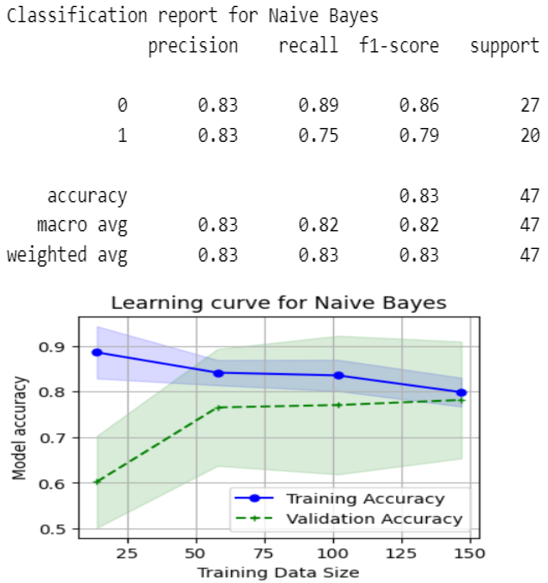
• MLFuzzyRoughSet: Improved Naive Bayes and Random Forest accuracies to 0.83, showcasing its robustness in handling uncertainty and imprecision.
• MLVarianceThreshold: Yielded accuracies of 0.72–0.77 across classifiers, underscoring the limitations of traditional variance-based selection compared to RST approaches.

Despite achieving 99% accuracy, we mitigated overfitting through the following:

• Stratified 10-fold cross-validation;
• L2 regularization in all classifiers (e.g., SVM, Neural Net);
• Hold-out validation (20% unseen data).

The consistency of results across folds (std. dev. $\le 0.03$) further supports model robustness. These results highlight the transformative potential of RST-based methods, enhancing accuracy, efficiency, and interpretability in machine learning, especially for imperfect or uncertain data.

6.2. Practical Implications and Future Directions

Our findings offer practical benefits for optimizing machine learning in fields like healthcare diagnostics and IoT systems. Methods like MLSpecialReduct and MLReduct distill minimal, discriminative feature sets, reducing computational load while preserving performance. Their inherent interpretability makes them ideal for explainable AI (XAI), fostering trust in high-stakes applications.

Future research should explore integrating RST with paradigms like deep learning, ensemble methods, or reinforcement learning to enhance performance further. Applying these techniques to diverse, real-world datasets—featuring imbalance, noise, or high dimensionality—will test their adaptability. Investigating their use in dynamic contexts, such as real-time or online learning, could enable adaptive models. Developing automated, scalable RST-based frameworks and evaluating their impact on interpretability and efficiency will drive progress toward advanced, transparent AI systems.

References

- Som, T.; Shreevastava, S.; Tiwari, A.K.; Singh, S. Fuzzy Rough Set Theory-Based Feature Selection: A Review. Math. Methods Interdiscip. Sci. 2020, 12, 145–166. [Google Scholar]
- Ye, J.; Sun, B.; Bao, Q.; Che, C.; Huang, Q.; Chu, X. A new multi-objective decision-making method with diversified weights and Pythagorean fuzzy rough sets. Comput. Ind. Eng. 2023, 182, 109406. [Google Scholar] [CrossRef]
- Singh, A.; Singh, A.; Sharma, H.K.; Majumder, S. Criteria selection of housing loan based on dominance-based rough set theory: An Indian case. J. Risk Finan. Manag. 2023, 16, 309. [Google Scholar] [CrossRef]
- Chen, R.-C.; Dewi, C.; Huang, S.-W.; Caraka, R.E. Selecting critical features for data classification based on machine learning methods. J. Big Data 2020, 7, 52. [Google Scholar] [CrossRef]
- Khosravi, F.; Izbirak, G. A framework of index system for gauging the sustainability of Iranian provinces by fusing Analytical Hierarchy Process (AHP) and Rough Set Theory (RST). Socio-Econ. Plan. Sci. 2024, 95, 101975. [Google Scholar] [CrossRef]
- Strasser, S.; Klettke, M. Transparent Data Preprocessing for Machine Learning. In Proceedings of the 2024 Workshop on Human-In-the-Loop Data Analytics, Santiago, Chile, 14 June 2024. [Google Scholar]
- Liu, H.; Zhou, M.; Liu, Q. An embedded feature selection method for imbalanced data classification. IEEE/CAA J. Autom. Sin. 2019, 6, 703–715. [Google Scholar] [CrossRef]
- Zong, Z.; Guan, Y. AI-driven intelligent data analytics and predictive analysis in Industry 4.0: Transforming knowledge, innovation, and efficiency. J. Knowl. Econ. 2024, 15, 1–40. [Google Scholar] [CrossRef]
- Islam, A.; Majumder, Z.H.; Miah, S.; Jannaty, S. Precision healthcare: A deep dive into machine learning algorithms and feature selection strategies for accurate heart disease prediction. Comput. Biol. Med. 2024, 176, 108432. [Google Scholar] [CrossRef]
- Theng, D.; Bhoyar, K.K. Feature selection techniques for machine learning: A survey of more than two decades of research. Knowl. Inf. Syst. 2024, 66, 1575–1637. [Google Scholar] [CrossRef]
- Singh, K.N.; Mantri, J.K. Clinical decision support system based on RST with machine learning for medical data classification. Multimed. Tools Appl. 2024, 83, 39707–39730. [Google Scholar] [CrossRef]
- Akram, M.; Zahid, S. Group decision-making method with Pythagorean fuzzy rough number for the evaluation of best design concept. Granul. Comput. 2023, 8, 1121–1148. [Google Scholar] [CrossRef]
- Chen, T.; Carlos, G. Xgboost: A scalable tree boosting system. In Proceedings of the 22nd Acm Sigkdd International Conference on Knowledge Discovery and Data Mining, San Francisco, CA, USA, 13–17 August 2016. [Google Scholar]
- Chen, H.; Li, T.; Fan, X.; Luo, C. Feature selection for imbalanced data based on neighborhood rough sets. Inf. Sci. 2019, 483, 1–2. [Google Scholar] [CrossRef]
- Zhang, X.; Yao, Y. Tri-level attribute reduction in rough set theory. Expert Syst. Appl. 2022, 190, 116187. [Google Scholar] [CrossRef]
- Manna, T.; Anitha, A. Hybridization of rough set–wrapper method with regularized combinational LSTM for seasonal air quality index prediction. Neural Comput. Appl. 2024, 36, 2921–2940. [Google Scholar] [CrossRef]
- Liu, T.; Yang, L. Financial risk early warning model for listed companies using bp neural network and rough set theory. IEEE Access 2024, 12, 27456–27464. [Google Scholar] [CrossRef]
- Lin, Q.; Chen, X.; Chen, C.; Garibaldi, J.M. Boundary-wise loss for medical image segmentation based on fuzzy rough sets. Inf. Sci. 2024, 661, 120183. [Google Scholar] [CrossRef]
- Fatima, A.; Javaid, I. Rough set theory applied to finite dimensional vector spaces. Inf. Sci. 2024, 659, 120072. [Google Scholar] [CrossRef]
- Singh, K.N.; Mantri, J.K. An intelligent recommender system using machine learning association rules and rough set for disease prediction from incomplete symptom set. Decis. Anal. J. 2024, 11, 100468. [Google Scholar] [CrossRef]
- Nayani, S.; Rao, P.S.; Lakshmi, D.R. Combination of deep learning models for student’s performance prediction with a development of entropy weighted rough set feature mining. Cybern. Syst. 2025, 56, 170–212. [Google Scholar] [CrossRef]
- Xu, W.; Yan, Y.; Li, X. Sequential rough set: A conservative extension of Pawlak’s classical rough set. Artif. Intell. Rev. 2025, 58, 9. [Google Scholar] [CrossRef]
- Kumari, N.; Acharjya, D.P. Data classification using rough set and bioinspired computing in healthcare applications—An extensive review. Multimed. Tools Appl. 2023, 82, 13479–13505. [Google Scholar] [CrossRef]
- Bohrer, J.d.S.; Dorn, M. Enhancing classification with hybrid feature selection: A multi-objective genetic algorithm for high-dimensional data. Expert Syst. Appl. 2024, 255, 124518. [Google Scholar] [CrossRef]
- Wang, C.; Wang, C.; Qian, Y.; Leng, Q. Feature selection based on weighted fuzzy rough sets. IEEE Trans. Fuzzy Syst. 2024, 32, 4027–4037. [Google Scholar] [CrossRef]
- Onu, O.P.; Muriana, B. Rough set theory and its applications in data mining. Technology 2024, 7, 84–92. [Google Scholar]
- Yadav, J. Fuzzy Logic and Fuzzy Set Theory: Overview of Mathematical Preliminaries. In Fuzzy Systems Modeling in Environmental and Health Risk Assessment; Elsevier: Amsterdam, The Netherlands, 2023; pp. 11–29. [Google Scholar]
- Guo, X.; Li, H. Attribute reduction algorithm of rough sets based on spatial optimization. arXiv 2024, arXiv:2405.09292. [Google Scholar]
- Pulinkala, G. Predicting Biomarkers/Candidate Genes Involved in iALL Using Rough Sets Based Interpretable Machine Learning Model. Master’s Thesis, Uppsala University, Uppsala, Sweden, 2023. Available online: https://www.diva-portal.org/smash/get/diva2:1803700/FULLTEXT01.pdf (accessed on 25 April 2025).
- Chen, Q.; Xie, L.; Zeng, L.; Jiang, S.; Ding, W.; Huang, X.; Wang, H. Neighborhood rough residual network–based outlier detection method in IoT-enabled maritime transportation systems. IEEE Trans. Intell. Transp. Syst. 2023, 24, 11800–11811. [Google Scholar] [CrossRef]
- Mwangi, I.K.; Nderu, L.; Mwangi, R.W.; Njagi, D.G. Hybrid interpretable model using roughset theory and association rule mining to detect interaction terms in a generalized linear model. Expert Syst. Appl. 2023, 234, 121092. [Google Scholar] [CrossRef]
- Guo, S.; Han, L.; Guo, Y. Advanced Technologies in Healthcare; Springer: Singapore, 2024. [Google Scholar]
- Chen, Q.; Zeng, L.; Ding, W. FRCNN: A Combination of Fuzzy-Rough-Set-Based Feature Discretization and Convolutional Neural Network for Segmenting Subretinal Fluid Lesions. IEEE Trans. Fuzzy Syst. 2024, 33, 350–364. [Google Scholar] [CrossRef]
- Kaya, Y.; Ramazan, T. Comparison of discretization methods for classifier decision trees and decision rules on medical data sets. Avrupa Bilim Teknol. Derg. 2022, 35, 275–281. [Google Scholar] [CrossRef]
- Dahouda, M.K.; Joe, I. A Deep-learned embedding technique for categorical features encoding. IEEE Access 2021, 9, 114381–114391. [Google Scholar] [CrossRef]
- Huang, L.; Qin, J.; Zhou, Y.; Zhu, F.; Liu, L.; Shao, L. Normalization techniques in training dnns: Methodology, analysis and application. IEEE Trans. Pattern Anal. Mach. Intell. 2023, 45, 10173–10196. [Google Scholar] [CrossRef] [PubMed]
- Li, F.; Chen, W. The Role of Attribute Normalization in Data Preprocessing for Machine Learning. Knowl.-Based Syst. 2019, 170, 1–10. [Google Scholar] [CrossRef]
- Cabello-Solorzano, K.; Ortigosa de Araujo, I.; Peña, M.; Correia, L.; Tallón-Ballesteros, A.J. The impact of data normalization on the accuracy of machine learning algorithms: A comparative analysis. In International Conference on Soft Computing Models in Industrial and Environmental Applications; Springer: Berlin/Heidelberg, Germany, 2023; pp. 344–353. [Google Scholar]
- Peng, H.; Long, F.; Ding, C. Feature selection based on mutual information criteria of max-dependency, max-relevance, and min-redundancy. IEEE Trans. Pattern Anal. Mach. Intell. 2005, 27, 1226–1238. [Google Scholar] [CrossRef] [PubMed]
- Takefuji, Y. Beyond XGBoost and SHAP: Unveiling true feature importance. J. Hazard. Mater. 2025, 488, 137382. [Google Scholar] [CrossRef]
- Li, Y.; Chen, C.-Y.; Wasserman, W.W. Deep feature selection: Theory and application to identify enhancers and promoters. J. Comput. Biol. 2016, 23, 322–336. [Google Scholar] [CrossRef]
- Cai, M.; Yan, M.; Wang, P.; Xu, F. Multi-label feature selection based on fuzzy rough sets with metric learning and label enhancement. Int. J. Approx. Reasoning 2024, 168, 109149. [Google Scholar] [CrossRef]
- Ke, G.; Meng, Q.; Finley, T.; Wang, T.; Chen, W.; Ma, W.; Ye, Q.; Liu, T.-Y. LightGBM: A Highly Efficient Gradient Boosting Decision Tree. Adv. Neural Inf. Process. Syst. 2017, 30, 3146–3154. [Google Scholar]