Abstract
Accurate characterization of subsurface geological structures, particularly those obscured by strong coal-seam reflections, is essential for hydrocarbon exploration in subtle reservoirs. Enhancing seismic resolution remains a pivotal technical challenge in addressing this demand. Here, we present a multitrace reflectivity inversion method guided by geological sparsity principles. This method establishes quantitative relationships between sparse inversion operators and the spatial positions of stratigraphic boundaries. Specifically, by integrating prior geological knowledge, such as stratigraphic boundaries and stable sedimentary structures, as constraint operators within the sparsity matrix, this method results in a geologically interpretable and robust inversion framework. Subsequently, we validated this method through synthetic data and field applications in a carbonate fracture–cavity reservoir in the Ordos Basin of western China. The enhanced seismic resolution demonstrates that our method effectively restores shielded reservoir reflections beneath coal seams. Clearer than conventional sparse inversion techniques, the coherence attribute of the enhanced seismic resolution reveals distinct fracture–cavity geometries. Moreover, integrated analyses of well logs, fracture–cavity characterization, and drilling production data further confirm the accuracy and reliability of the inversion results. In conclusion, this method effectively leverages accurate geological structural information to enhance localized seismic resolution, thereby providing robust support for the exploration of subtle hydrocarbon reservoirs.
1. Introduction
In the exploration of complex hydrocarbon reservoirs and subtle reservoirs, enhancing seismic resolution is essential [1]. This can be achieved through multiple approaches, including data acquisition, processing [2,3], and post-stack inversion techniques. As a core method for quantitative reservoir characterization, post-stack seismic inversion significantly improves thin-bed identification and reservoir prediction accuracy by transforming seismic data into physical property parameters such as impedance. With the development of multi-physics integrated exploration [4], interdisciplinary methods like gravity and electromagnetic inversion have become important supplements to seismic inversion [5].
Post-stack seismic inversion is inherently ill posed, requiring regularization constraints to stabilize the solution [6]. The selection of regularization terms should align with the desired characteristics of the inversion results. Specifically, L2-norm (minimizing the sum of squared values) regularization is suitable for Gaussian-distributed solutions; L1-norm (minimizing the sum of absolute values) [6,7] or Lp-norm [8,9] constraints apply to sparse signals; Tikhonov regularization [10] enforces smoothness; and total variation regularization [11] preserves blocky structures. Moreover, advanced techniques like maximum entropy and Cauchy constraints [6] can also be implemented based on geological requirements. However, these constraints primarily optimize vertical structures in single-trace inversion, which faces inherent limitations—a trade-off between sparsity weight and noise suppression: reduced weights enhance resolution but weaken noise attenuation, whereas stronger denoising causes signal oversmoothing. Furthermore, single-trace inversion may introduce spurious high-frequency components when layer thickness falls below one-quarter wavelength, necessitating spatial constraints to ensure solution reliability.
Multitrace inversion extends single-trace methods by adding lateral constraints, optimizing both vertical and horizontal structures through regularization, alongside data fidelity and sparsity constraints. Key developments include the following: Idier and Goussard [12] used Markov–Bernoulli fields for 2D reflectivity; Kaaresen and Taxt [13] combined sparse priors with seismic data in Bayesian deconvolution; and Heimer and Cohen [14] modeled trace correlations via Markov fields. Kazemi and Sacchi [15] introduced sparse blind deconvolution; Gholami [16] preserved blocky features with total variation. Pan [17] implemented frequency-domain sparse inversion. Wang [18] enhanced continuity with predictive filtering. Yuan [19] used block-sparse learning for reflectivity. Wu [20] improved accuracy with structural constraints. Du [21] and Xing [22] outperformed sparse spike inversion using data-driven constraints. Garabito [23] and Zhang [24] optimized reflectivity pulses via simulated annealing. Wang [25], Hamid [26], and Bruno [27] integrated dip and fault data. Aghamiry [28] and Chen [29] developed adaptive operators. Li [30] and Chen [31] employed deep learning for geological constraints in Bayesian inversion, reducing non-uniqueness while maintaining geological consistency.
Current multitrace structural-constrained inversion methods predominantly utilize spatial information solely for initial model construction [26]. Although the initial model inherently embodies lateral constraints, these constraints either remain inactive during inversion or merely prevent excessive deviation from the initial model, without effectively exploiting intertrace spatial relationships and structural features in seismic data [30]. Consequently, such approaches essentially remain single-trace inversions. Furthermore, existing multitrace methods that incorporate lateral constraints under specific assumptions predominantly formulate regularization terms from mathematical perspectives or seismic-derived features, yet fail to adequately integrate available geological characteristics. This may yield geologically implausible results, particularly when underlying assumptions significantly deviate from actual subsurface conditions.
In this paper, our objective is to develop geologically guided operators that are more closely aligned with actual subsurface conditions, based on prior geological knowledge. Firstly, we provide an in-depth analysis of multitrace sparse inversion, revealing that the sparse matrix in the inversion operator is related to the stratigraphic boundaries. Based on this insight, we propose a reflectivity inversion method guided by geological sparse criteria. This method innovatively incorporates geological guidance information into the sparse matrix, establishing a more accurate and stable structural constraint framework. Subsequently, we apply this method in the field data from a carbonate sedimentary environment in western China. The proposed method restores reflection signals under strong coal-bed reflections, significantly improving resolution and clarifying reservoir structures. Furthermore, through comprehensive quality control analysis, the accuracy and reliability of the interpretation results are verified. Therefore, this method provides robust technical support for the detailed interpretation of complex oil and gas reservoirs.
2. Methodology
This section systematically develops the proposed geologically guided sparse inversion framework through four key components. We first introduce the mathematical foundation of classical single-trace reflectivity sparse inversion. Subsequently, we analyze the spatial correlation between sparse vectors and reflection interfaces in single-trace inversion. Building on this, we extend the analysis to multitrace scenarios by investigating the structural characteristics of sparse matrices. Finally, we propose a novel geological-guided sparse matrix construction method that integrates spatial geological structural constraints to enhance inversion accuracy.
2.1. Principle of Reflectivity Sparse Inversion
Reflectivity is a parameter that represents the difference in the physical properties of two rock layers. It is presented in the form of a pulse sequence and has a wide-band frequency spectrum. The seismic data collected are influenced by Earth filtering, and the seismic wavelet is band-limited. Reflectivity inversion eliminates the effects of stratigraphic filtering and estimates the true spatial structure of the subsurface layers from seismic data, aiming to enhance the resolution of seismic data. Assuming that the seismic wavelet is stationary within a certain spatiotemporal range, a convolution model can be used in the time domain to represent it:
where denotes convolution operation, denotes the seismic record, represents the seismic wavelet, represents the impulse response, commonly referred to as the reflectivity, and denotes the noise. The equation can be rewritten in matrix form, involving matrix multiplication:
where represents the seismic record, represents the wavelet matrix, represents the reflectivity, and represents the noise. The wavelet matrix is formed by arranging seismic wavelets and reflects the inversion and time-shift processes in the convolution model Equation (1).
In seismic exploration, inversion is generally expressed as follows:
where is the inversion operator. For the noisy convolution model, there is an objective function:
where is the regularization parameter, which balances the weight between the data fitting term and the sparsity constraint term. is the norm order of the sparsity constraint, typically set as , and controls the sparsity of the reflectivity. The symbol denotes the Lp-norm, which measures the sparsity of the reflectivity vector. By adjusting these parameters, the inversion results can be optimized to better align with the prior knowledge of geological structures.
In the case of noisy data, based on the least squares method, the inversion reflectivity can be expressed as follows:
where is a sparse matrix. According to Equation (3), the least squares inversion operator for data can be expressed as follows:
Based on different solution algorithms, both the inversion operator and the inversion reflectivity will be iteratively updated continuously. In this paper, the alternating direction method of multipliers (ADMM) solution algorithm [32] is taken as an example. We introduce an auxiliary variable and rewrite the objective function as follows:
In this context, we formulate the Lagrangian equations to solve the aforementioned system of equations. The augmented Lagrangian function is defined as follows:
where is the Lagrange multiplier, and is the penalty parameter. After convergence, the closed-form solution for can be expressed in terms of , , and as follows:
2.2. Sparse Vector in Single-Trace Inversion
According to Equation (1), taking 1D reflection coefficient inversion as an example, Figure 1 illustrates the results of the inversion operator (Figure 1a), noisy data (Figure 1b) with 10% noise, and the inversion reflectivity (Figure 1c) after 100 iterations. After 100 iterations, the inversion operator exhibits two horizontally distributed values at the positions corresponding to the reflectivity (at positions 33 and 66), while the values at other positions converge to a mean value. It can be observed that there is a certain correlation between the inversion operator and the positions of the reflection coefficients.
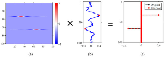
Figure 1.
Damped least squares schematic with noise (, , ). (a) Inversion matrix ; (b) noisy data with 10% noise; and (c) inversion reflectivity . This figure validates the noise-robust interface localization capability of single-trace sparse inversion, illustrating the spatial correlation between operator and reflectivity during iterative optimization.
According to Equation 6, as shown in Figure 2, the inversion operator (Figure 2c) is obtained by multiplying the inverse of (Figure 2a) with the transpose of the wavelet matrix (Figure 2b). Since is only related to the seismic wavelet, it can be inferred that the inverse of () determines the positions of the reflection coefficients.
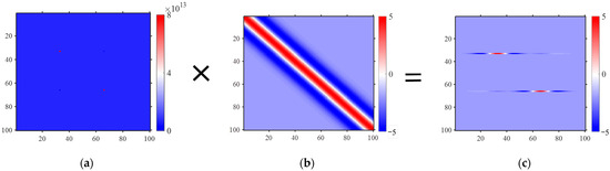
Figure 2.
Inversion matrix schematic (, , ). (a) The inverse matrix of ; (b) transposed wavelet matrix ; and (c) inversion matrix . This figure illustrates the mathematical construction of the inversion operator through the matrix decomposition process. It reveals how the inverse operation of governs the spatial distribution of reflectivity coefficients, independent of the wavelet matrix .
For further analysis, () is decomposed into (Figure 3a) and (Figure 3b) diagonal elements (representing spatial constraint intensity), which significantly exceed those of (reflecting wavelet autocorrelation energy). Since (λ)−1 dominates the matrix inversion process, the spatial resolution of inversion operator is determined by ’s constraint pattern: high diagonal elements in correspond to strong regularization zones (suppressing spurious reflections), while low elements indicate weak constraint regions (preserving true interfaces). Furthermore, the band-limited nature of provides limited positional information, whereas encodes prior spatial constraints of reflectivity through its diagonal distribution. This mathematical representation of geological information establishes as the primary carrier of positional information. Consequently, the significant dominance of ’s diagonal element magnitudes enables it to govern the positional information of reflectivity.
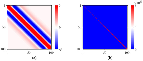
Figure 3.
Schematic of the decomposition of the inverse matrix of (, , ). (a) Matrix ; (b) matrix . The figure further reveals that the diagonal numerical superiority of the regularization sparse matrix dominates the spatial constraints of reflectivity coefficients.
We define the diagonal elements of the matrix as a vector :
Clearly, the vector in the aforementioned equation is influenced by various factors, such as sparsity assumptions, the number of iterations, and others. Through multiple tests, we have observed a stable relationship between the vector and the positions of the reflectivity. Taking the scenario with an Lp-norm of 0.8 as an example, Figure 3 illustrates the iterative process of the vector . During the first iteration, due to the influence of seismic data and mathematical sparsity assumptions, the distribution of is relatively uniform, with low values near both reflectivity positions (at time positions 33 and 66) and non-reflectivity positions (Figure 4a). As the iterations progress, the values of oscillate and change. By the 10th iteration, the distribution of undergoes a significant transformation (Figure 4b), maintaining low values near reflectivity positions while exhibiting higher values near non-reflectivity positions. By the 100th iteration, the distribution of shows two distinct minima, which correspond to the positions of the reflectivity (Figure 4c). Based on this, we can summarize the relationship between the sparse vector and the reflectivity positions: low values of appear at reflectivity positions, while high values appear at non-reflectivity positions.
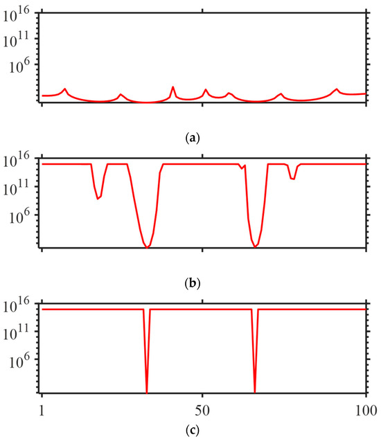
Figure 4.
Relationship between vector and reflectivity position under different iteration counts (, ). (a) Vector after 1 iteration; (b) vector after 10 iterations; and (c) vector after 100 iterations. The figure illustrates the evolution of sparse vector during iterative inversion: as iterations progress, develops stable minima at reflectivity positions (e.g., samples 33 and 66), demonstrating the spatial constraint stability of geological sparse criteria.
2.3. Sparse Matrix in Multitrace Inversion
In multitrace inversion, the sparse matrix is composed of the sparse vectors q from each trace, representing the vertical sparse expression of seismic data:
where represents the number of seismic traces, and the sparse matrix is jointly constrained by the seismic data and mathematical sparsity assumptions.
To analyze the characteristics of the sparse matrix , this section designs a 2D wedge-shaped reflectivity model (Figure 5a). Seismic data are synthesized by convolving the model with a 30 Hz Ricker wavelet (Figure 5b), and 10% random Gaussian white noise is added to each trace (Figure 5c).
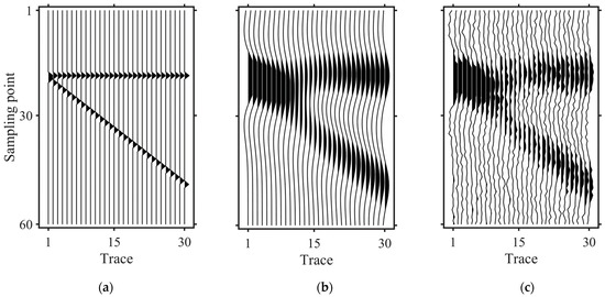
Figure 5.
The wedge model. (a) Reflectivity. (b) Synthetic seismic data. (c) Noisy seismic data with 10% random noise. The figure displays the designed wedge-shaped reflectivity model and its noisy seismic data, aiming to validate the adaptability of constraint operators to thin interbeds and noise under varying conditions.
Using the noisy seismic data for multitrace reflectivity inversion, and taking the Lp norm of 0.8 as an example, Figure 6 illustrates the changes in the sparse matrix and the inversion results at different iteration counts. During the first iteration, the positional information in (Figure 6a) resembles the boundaries of the seismic data, and the inversion result (Figure 6d) appears relatively blurred. By the 10th iteration, (Figure 6b) begins to exhibit wedge-shaped structural features, although the boundaries remain somewhat unclear, while the inversion result (Figure 6e) achieves a higher resolution. By the 100th iteration, (Figure 6c) demonstrates a sparse wedge-shaped structural characteristic, and as the precision of improves, the accuracy and resolution of the inversion reflectivity (Figure 6f) are significantly enhanced.
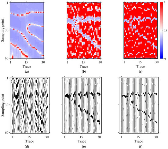
Figure 6.
Results of sparse matrix and inversion under different iteration counts (, ). (a) after 1 iteration; (b) after 10 iterations; (c) after 100 iterations; (d) inversion after 1 iteration; (e) inversion after 10 iterations; and (f) inversion after 100 iterations. The figure validates the progressive enhancement of geological constraints on reflectivity spatial distribution and resolution through iterative optimization, demonstrated by structural evolution of sparse matrix and corresponding inversion results.
Through the analysis in this subsection, it is found that the two-dimensional sparse matrix in multitrace inversion structurally aligns with the true reflectivity model, accurately resolving stratigraphic boundaries and lateral depositional continuity. The sparse vector exhibits a direct spatial correspondence with reflectivity positions, where its minima systematically coincide with reflection interfaces. This positional relationship extends to the composite sparse matrix , which quantifies the subsurface architecture through vertical impedance contrasts and lateral geological patterns.
2.4. Construction of the Geological-Guided Sparse Matrix
The analysis in the previous section on the relationship between the sparse matrix and the multitrace reflectivity inversion results provides guidance for optimizing these results. To this end, we gradually introduce geological structures, stratigraphic boundaries, and the internal information of geological bodies to construct a geological-guided sparse matrix . By integrating existing geological knowledge into the inversion process, the inversion results can be further improved.
First, the geological structure constraint matrix is introduced. This matrix does not have sparse requirements in the vertical direction, and maintains good continuity in the horizontal direction, which can reflect the approximate spatial distribution information of the subsurface [33]. The geological structure constraint matrix is as follows:
where represents the geological structure constraint matrix, which reflects the basic structural morphology underground. is the algorithm used to extract structural constraints, is the input seismic data, and is the length of the time window when extracting the structure. The algorithm for extracting structural constraints can determine the possible locations of reflectivity by inputting seismic data. The output range is larger than the actual range of reflectivity. The lower the value, the higher the likelihood of the presence of reflectivity. This is consistent with the relationship between the vector and the reflectivity position.
The extracted structures are dependent on the extraction radius . When is small, the wedge-shaped reflection structures exhibit strong discontinuities (Figure 7a); when is appropriate, the extracted structural information aligns well with the boundaries of the seismic data (Figure 7b); and when is excessively large, the structural information introduces artifacts at the boundaries, and the wedge-shaped reflection structures exhibit noticeable computational segmentation artifacts (Figure 7c).
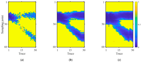
Figure 7.
Geological structure constraint matrix extracted from noisy data. (a) ; (b) ; and (c) . The figure demonstrates the impact of different extraction radius parameters on the structural characteristics of the constraint matrix .
Subsequently, stratigraphic boundary information is further introduced to enrich the geological information characterized in the matrix. These stratigraphic boundaries refer to the interfaces between different geological layers, marking the division of sedimentary or metamorphic events throughout geological history. We use prior information from well logs and mud logs to identify the exact locations of these stratigraphic boundaries, which are then incorporated as geological constraints during the inversion process. Afterwards, stratigraphic boundary information is incorporated into the geological structure constraint matrix, as follows:
where represents the number of seismic traces, and denotes the position of the stratigraphic boundaries. Figure 8b shows the constraint matrix adding stratigraphic boundaries (), where the black straight line indicates the added stratigraphic boundaries. Incorporating stratigraphic boundaries after structure extraction can, to some extent, mitigate the inaccuracies of the structure extraction algorithm. After adding the interface information, the multi-structural constraints become more comprehensive, which is beneficial for precise inversion.
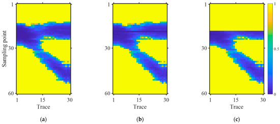
Figure 8.
Geological-guided sparse matrix extracted from noisy data (). (a) Structure-constrained matrix ; (b) with added stratigraphic boundary information; and (c) with added geological prior information. The figure illustrates the construction of the geologically guided sparse matrix by progressively incorporating structural constraints, stratigraphic boundaries, and internal geological body information. It demonstrates how geological priors optimize the spatial distribution of inversion results.
Finally, the internal geological body information is introduced. The equation for adding internal geological body information to the constraint matrix is as follows:
where also denotes the position range of the internal geological body. Figure 8c shows the geologically guided constraint matrix adding internal geological body information (). It can be observed that the geological information in is further clarified, and the constraints of the geological information become more pronounced.
2.5. Multitrace Reflectivity Inversion Based on Geologically Guided Sparse Criteria
Building upon the aforementioned analysis, the iterative inversion framework demonstrates that under the sparsity assumption of seismic data, the sparse reflection coefficient matrix progressively converges toward the true subsurface reflectivity model. Leveraging this mechanism, we propose a multitrace reflectivity inversion method based on the geologically guided sparsity criterion, which integrates data-driven sparsity regularization with geological prior knowledge to enhance the fidelity of subsurface parameter estimation. The specific inversion equation is as follows:
The geologically guided sparse matrix is expressed as follows:
where is the Kronecker product, and is the constructed geological steering matrix, which is used to adjust the extreme value distribution of the column vectors in the sparse matrix . Figure 9 shows the inversion results of the reflectivity for the noisy synthetic seismic data based on the geological-guided sparsity criterion and the geological-guided sparse matrix . Overall, denotes the original sparse matrix constructed without geological constraints, and represents the geologically guided sparse matrix obtained by applying structural constraints through the Kronecker product with .
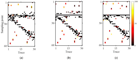
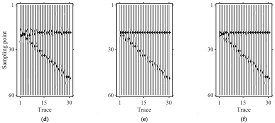
Figure 9.
Inversion of noisy data using structure constraint extracted from noisy data ( , , , ). (a) Structure-constrained matrix ; (b) stratigraphic boundary structure-constrained matrix ; (c) geological prior information structure-constrained matrix ; (d) inversion using structure-constrained matrix; (e) inversion using stratigraphic boundary structure-constrained matrix; and (f) inversion using geological prior information structure-constrained matrix. The figure demonstrates the progressive construction of geologically guided sparse matrix L through sequential incorporation of structural, stratigraphic, and geobody constraints. The corresponding inversion results validate the effectiveness of geological constraints in enhancing resolution and restoring subtle reservoir details.
In Figure 9a, structural information is incorporated into the matrix. In Figure 9b, =stratigraphic boundaries are added to the matrix at the position τ = 19, where the stratigraphic position consistently maintains low values. In Figure 9c, the internal features of the geological body are added to the matrix, effectively removing anomalies around the stratigraphic position at τ = 19. Comparing the geologically guided sparse matrix in Figure 9a–c with the sparse matrix , it is evident that the wedge-shaped features are more distinctly characterized in . Furthermore, as more specific prior geological information is added, the geological features in the matrix become more deterministic and clearer. Figure 9d shows the inversion result based on the matrix from Figure 9a, Figure 9e shows the inversion result based on the matrix from Figure 9b, and Figure 9f shows the inversion result based on the matrix from Figure 9c. With the inclusion of prior geological information, the resolution of the inversion results gradually improves, and the separability of the wedge-shaped strata progressively enhances. In Figure 9f, the wedge-shaped model becomes distinguishable at an interval of just 6 sampling points.
2.6. Methodology Flow and Data Description
In order to effectively enhance seismic resolution, this paper proposes multitrace reflectivity inversion based on geologically guided sparse criteria. The method flow is illustrated in Figure 10. For the raw seismic data from the study area, the geological constraint matrix is first constructed by extracting structural features and integrating stratigraphic boundaries and geobody information. Then, the reflectivity is solved via objective function construction and ADMM iteration, with convergence checks determining the final inversion result.
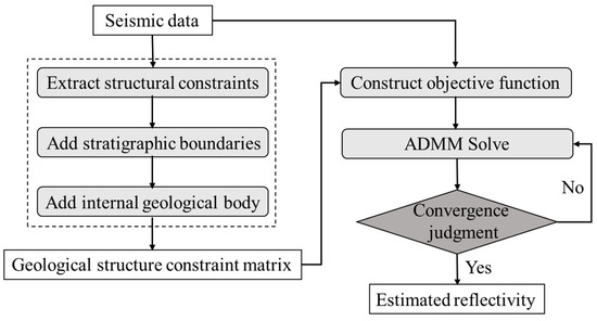
Figure 10.
The flowchart of multitrace reflectivity inversion based on geologically guided sparse criteria.
For the development, testing, and validation of the method, various types of data were collected to support the analysis. High-quality post-stack seismic data were first used to evaluate the improvement in seismic resolution provided by the proposed inversion method. In addition, lithological data from mud logging, wireline logging curves (including Gamma Ray, Density logs, and the reflectivity profiles calculated from the logging data), and well stratigraphy were integrated to define the spatial distribution of coal seams. These datasets served as geological constraints during the inversion process and were also used to validate the inversion results. Furthermore, production data from development wells, reflecting the performance of different well locations, were incorporated to cross-validate the geological reliability of the reservoir characterization outcomes.
3. Results
The study area of this field data is located in the Ordos Basin of western China, a major hydrocarbon-producing region characterized by a carbonate rock sedimentary environment. The primary lithology of the target reservoir is dolostone and limestone, which are of significant importance in hydrocarbon exploration due to their fracture porosity and cavernous structures. However, the target layer is overlaid by a coal seam approximately 10 m thick, which has a high acoustic impedance. The strong reflections from the overlying coal seams suppress and shield the effective reflection signals from the reservoir, interfering with the detection of the reservoir’s internal structures. The complex fracture–cavity geometries within the carbonate formation, coupled with the low resolution of seismic data, present significant challenges to accurately characterizing the reservoir.
Given the pronounced thickness, extensive lateral extension, and internal stability of coal seam, we integrate well-logging lithology data, petrophysical interpretation, and seismic horizon interpretation to precisely characterize the spatial distribution of coal seams within the stratigraphic framework. Building upon this foundation, by incorporating the coal-seam distribution as a geological steering matrix into the reflectivity inversion process, this method is expected to enhance resolution and effectively restore reservoir reflections affected by coal-seam reflection shielding effects.
Both our proposed reflectivity inversion method based on geologically guided sparse criteria and the conventional sparse reflectivity inversion method were tested on field data. To better align with field data processing scenarios, the inversion results were convolved with the seismic wavelet to synthesize high-resolution seismic data for comparison. Figure 11a shows the profile of inline 7710 from the observed seismic data, revealing the relatively low resolution of the original data (indicated by black arrows). Additionally, the reservoir (highlighted by the green dashed box) exhibits weak reflection signals due to shielding by the overlying coal seams. Figure 11b presents the high-resolution seismic data obtained after conventional sparse inversion processing. Compared to the original data, the resolution has improved, but the continuity of the strata remains poor, with some stratigraphic layers still overlapping along the same reflection axis, making it difficult to distinguish between them, especially at the reservoir location beneath the coal seam. In Figure 11c, we present the results after applying the geologically guided sparsity criteria inversion method. Compared to the conventional method, the resolution is significantly improved, with much clearer details of the strata. The continuity of the strata is notably enhanced, especially the reflection of the reservoir, which shows a marked improvement in clarity and allows for distinct differentiation of the reflection axes of the coal and reservoir layers.
Figure 11.
Comparison of inversion results from field data. (a) Observed seismic data profile; (b) high-resolution profile from sparse inversion; and (c) high-resolution profile from geologically guided sparse criteria inversion. The figure compares field seismic data, conventional sparse inversion, and geologically guided inversion to validate the method’s effectiveness in restoring shielded reservoir (green dashed box) reflections and enhancing stratigraphic resolution under coal-seam interference (indicated by arrows).
To further assess the effectiveness of the inversion methods, we zoomed in on the area around the coal seam and reservoir for detailed analysis. Figure 12 shows the seismic data, with the black line indicating the well position and the blue curve representing the gamma curve of the blind well. The yellow band marks the coal seam, while the red dashed box highlights the fracture–cavity reservoir primarily composed of limestone. Figure 12a presents the observed seismic data, where the strong reflection amplitude from the coal seam is evident, along with high gamma values. Below the coal seam, in the limestone reservoir section, the gamma values remain very low, and there is almost no visible stratigraphic information, with the seismic reflection signals being very weak. Figure 12b displays the high-resolution seismic data obtained after sparse inversion processing. Some new geological features below the coal seam emerge (as indicated by the green arrows), but their continuity is poor. Although some signal restoration occurs at the reservoir location, the resolution is insufficient to clearly distinguish the seismic reflection axes of the coal seam and the reservoir. In Figure 12c, we present the high-resolution seismic data obtained after applying the geologically guided sparsity criteria inversion method. Below the coal seam, continuous stratigraphic information is much clearer, demonstrating a significant improvement in resolution compared to the sparse inversion result (as shown by the green arrows). At the reservoir location, the sparse inversion method failed to effectively restore the signal, whereas our method successfully recovered the signals below the strong amplitude axis of the coal seam, clearly distinguishing the reservoir from the coal seam. This results in a well-defined lateral distribution of the restored geological body (as indicated by the black arrows in Figure 12c).
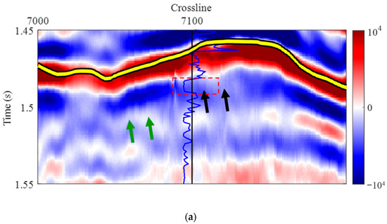
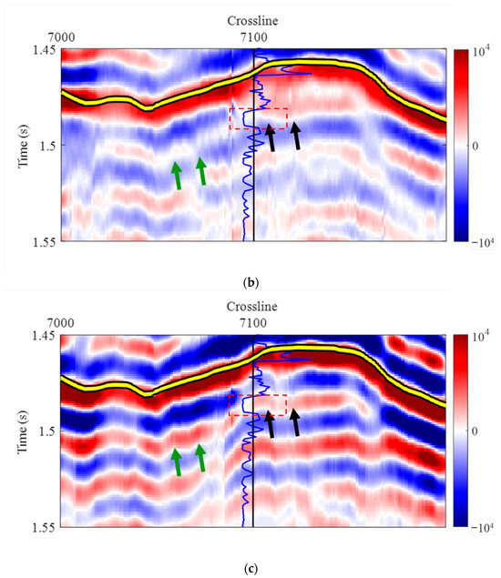
Figure 12.
Zoomed-in comparison of inversion results. (a) Observed seismic data profile; (b) high-resolution profile from sparse inversion; and (c) high-resolution profile from geologically guided sparse criteria inversion. The figure shows the seismic data, with the black line indicating the well position and the blue curve representing the gamma curve of the blind well. The yellow band marks the coal seam, while the red dashed box highlights the reservoir. The figure validates the effectiveness of the proposed method in restoring masked reservoir reflections beneath coal-seam interference (red dashed box) and enhancing stratigraphic resolution (indicated by arrows) through localized magnification of comparative profile sections.
For field data, the fidelity of the inversion is crucial for accurate geological interpretation. To validate the geologically guided sparsity criteria reflectivity inversion method, we conducted quality control using the blind well located at inline 7710 and crossline 7140, as shown in Figure 13. The left side of the profile represents the depth coordinate, while the right side shows the two-way travel time coordinate. The first column on the left displays the lithology, which includes five different lithologies; the black curve represents the well’s gamma curve, the blue curve corresponds to the RHOB (density) curve, and the red curve illustrates the reflectivity derived from the well data, filtered to match the seismic data bandwidth. The colored dashed lines represent the geological horizons T1 to T5, as interpreted from the well logs. A thick coal seam is located above T1, and the interval between T2 and T3 corresponds to a thick fractured–vuggy limestone reservoir, which is a key target for hydrocarbon exploration.
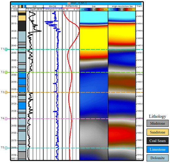
Figure 13.
Validation of inversion results using a blind well in the study area. The figure validates the reliability of the geologically guided sparse criteria inversion method through blind well quality control. It demonstrates restored reservoir reflections beneath coal seams with strong consistency between inversion results, well logs (lithology, gamma, and reflectivity), and interpreted horizons.
The profile on the left shows the observed seismic data, while the profile on the right displays the inversion results. Comparative analysis reveals that the observed seismic data exhibit a relatively low resolution due to the strong reflection interference from the coal seam. The amplitude masking effect leads to almost no distinct reflective signals in the reservoir interval (T2–T3). However, after applying the new inversion method, the overall resolution significantly improves, and the signals from the reservoir interval (T2–T3) are effectively restored. Additionally, the restored stratigraphic information aligns well with the lithology (limestone), gamma (low values), reflectivity (high values), and interpreted geological horizons (T2–T3), demonstrating that the results obtained by the new inversion method exhibit a high degree of credibility.
Building upon high-resolution processed seismic data, structural characterization of the target reservoir beneath the coal seam was conducted to further validate the accuracy of the inversion results. Figure 14a and Figure 14b display the coherence attribute horizon slices of the target layer before and after inversion, respectively. Comparative analysis demonstrates that the original coherence attributes (Figure 14a), affected by strong reflection shielding effects from overlying strata, exhibit poorly resolved geological features including faults and karst cavities. In contrast, the high-resolution coherence slice (Figure 14b) reveals enhanced geological details, clearly delineating multiple NE-SW-trending faults with associated secondary fracture systems. The spatial relationships between karstic voids and fault networks are markedly improved, with substantially elevated identification accuracy. Notably, high-productivity gas wells (marked by red circles) in this interval are preferentially distributed in areas with well-developed fracture–cave reservoirs. The gas productivity of these wells shows a strong correlation with interconnected dissolution channels and fracture networks, which constitute effective reservoir spaces. Validation confirms superior spatial correspondence between high-yield well locations and favorable fractured–vuggy reservoirs in the high-resolution coherence slice compared to the original data.
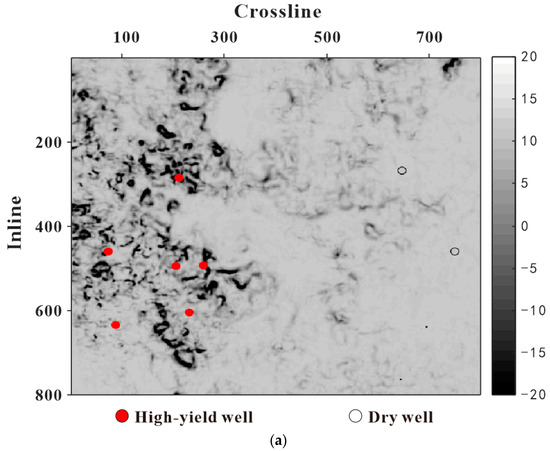
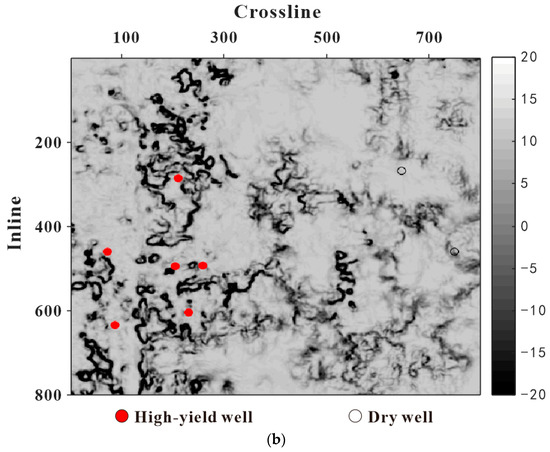
Figure 14.
Comparison of C3 coherence attribute slices of the target reservoir original data and inversion data: (a) C3 coherence attribute slice from original data; (b) C3 coherence attribute slice from inversion data. The figure demonstrates the enhanced reservoir characterization from inversion: the original coherence slice (a) shows obscured features under coal-seam interference, while the inversion result (b) clearly reveals fault and karst systems, validating the method’s effectiveness.
4. Discussion
The multitrace reflectivity inversion method based on geological sparsity criteria proposed in this paper demonstrates significant advantages in improving inversion accuracy and stability. By integrating geological guidance information into the sparse matrix, this method not only optimizes the inversion results but also achieves promising outcomes in practical data applications.
The inversion method proposed in this paper differs from conventional geological structural constraint methods. Conventional methods primarily derive structural information through mathematical or physical formulas, such as calculating total variation regularization [16,34] or using dip attributes [35,36]. And the extracted structural constraints are directly applied to the inversion objective function. Therefore, the structural information above may not align with the actual subsurface conditions. Moreover, as variables during the iterative process, the structural constraints are computationally unstable. In contrast, our geological-guided approach introduces prior geological knowledge and geological interpretation, providing guidance information. The prior geological information is directly incorporated into the inversion matrix. Here, known geological insights are quantitative, and they influence the iterative process but do not change during the process. This ensures greater stability of the prior geological information.
Despite these advantages, several limitations should be noted. First, the effectiveness of the geologically guided inversion largely depends on the availability, accuracy, and completeness of the prior geological knowledge ( matrix). In regions where geological interpretation is incomplete, uncertain, or incorrect, the inversion results may still be affected by artifacts or misinterpretations. Moreover, acquiring high-quality geological information requires extensive analysis and expertise, which may not always be feasible in every field area. Secondly, although the sparse matrix construction enhances seismic resolution, the performance of the inversion remains inherently limited by the choice of the initial sparse basis , particularly in highly heterogeneous geological environments. This is because the static sparse basis may not fully capture local complexity. Future work should focus on developing adaptive sparse representations and dynamically updated geological constraints to further improve the robustness and generalization of the inversion process.
In addition, for specific geological targets such as coal seam characterization, integrating targeted predictive techniques developed by other scholars [37,38] could provide more accurate geological priors. Combining such targeted geological prediction with the proposed geologically guided inversion framework represents a promising avenue for further improving inversion precision. Furthermore, the current study focuses solely on seismic data. Future research will prioritize multi-physics data integration, such as coupling seismic, electromagnetic, and gravity data within a joint inversion framework, to achieve more comprehensive and accurate characterization of complex geological structures and subtle hydrocarbon reservoirs.
5. Conclusions
The geologically guided sparse criteria-constrained multitrace reflectivity inversion method proposed in this study effectively addresses the resolution limitations in imaging subtle reservoirs obscured by strong coal-seam reflection shielding. Through systematic theoretical analysis and practical applications, the following key conclusions are drawn.
Theoretical analysis reveals an intrinsic correlation between the sparse matrix in the inversion algorithm and stratigraphic interface positions: minima in the sparse vector q systematically correspond to reflection interfaces, while the composite matrix quantitatively characterizes subsurface structural patterns through vertical impedance contrasts and lateral depositional continuity. This provides the theoretical foundation for integrating geological prior information into inversion operators.
The innovatively constructed geologically guided sparse matrix integrates three geological elements: (a) a macrostructural framework extracted from seismic data attributes, (b) interface spatial positions constrained by stratigraphic boundaries, and (c) internal distributions of geological bodies calibrated with well-log data. This comprehensive constraint framework achieves simultaneous optimization of data fidelity and geological plausibility.
Field application in a western carbonate fracture–cavity reservoir demonstrates significant improvements: outperforming conventional sparse inversion, this method notably enhances vertical resolution, thereby successfully restoring reservoir responses shielded by strong coal-seam reflections and achieving clear imaging of fracture–cavity geometries in inverted sections. Integrated analysis of drilling production data and inversion results confirms strong consistency between interpreted fracture–cavity spatial configurations and actual development dynamics, providing reliable support for precise characterization of subtle reservoirs.
This methodology establishes a new paradigm for interpretable geological model-driven multitrace seismic inversion. Future research should focus on three directions: (1) developing a multi-physics coupled inversion framework for anisotropic media, (2) integrating multivariate information and deep learning algorithms for the intelligent extraction and dynamic constraint of geological features, and (3) creating geological evolution inversion modules for time-lapse seismic data. Therefore, through continuous algorithmic optimization, this approach holds promising potential for broader applications in complex hydrocarbon reservoir exploration and development.
Author Contributions
S.C.: writing—original draft; Y.X.: methodology; J.F.: data curation; Y.Y.: formal analysis; S.Y.: supervision. All authors have read and agreed to the published version of the manuscript.
Funding
This work was supported in part by the National Key Research and Development Program of China (2018YFA0702504), and in part by the R&D Department of China National Petroleum Corporation (2022DQ0604-01).
Institutional Review Board Statement
Not applicable.
Informed Consent Statement
Not applicable.
Data Availability Statement
The original contributions presented in this study are included in the article. Further inquiries can be directed to the corresponding author.
Conflicts of Interest
All authors declare that the research was conducted in the absence of any commercial or financial relationships that could be construed as potential conflicts of interest. The funder was not involved in the study design, collection, analysis, interpretation of data, writing of this article, or decision to submit it for publication.
References
- Yilmaz, O. Seismic Data Analysis; Society of Exploration Geophysicists: Tulsa, OK, USA, 2001. [Google Scholar] [CrossRef]
- De Gori, P.; Cimini, G.B.; Chiarabba, C.; De Natale, G.; Troise, C.; Deschamps, A. Teleseismic Tomography of the Campanian Volcanic Area and Surrounding Apenninic Belt. J. Volcanol. Geotherm. Res. 2001, 109, 55–75. [Google Scholar] [CrossRef]
- Zollo, A.; Gasparini, P.; Virieux, J.; le Meur, H.; de Natale, G.; Biella, G.; Boschi, E.; Capuano, P.; de Franco, R.; Dell’Aversana, P.; et al. Seismic Evidence for a Low-Velocity Zone in the Upper Crust Beneath Mount Vesuvius. Science 1996, 274, 592–594. [Google Scholar] [CrossRef]
- Zollo, A.; D’Auria, L.; De Matteis, R.; Herrero, A.; Virieux, J.; Gasparini, P. Bayesian Estimation of 2-DP-Velocity Models from Active Seismic Arrival Time Data: Imaging of the Shallow Structure of Mt Vesuvius (Southern Italy). Geophys. J. Int. 2002, 151, 566–582. [Google Scholar] [CrossRef]
- Aiello, G.; Marsella, E. Marine Geophysics of the Naples Bay (Southern Tyrrhenian Sea, Italy): Principles, Applications and Emerging Technologies. Geophys. Princ. Appl. Emerg. Technol. 2016, 1, 61–121. [Google Scholar]
- Wang, Y. Seismic Inversion: Theory and Applications; Wiley-Blackwell: Hoboken, NJ, USA, 2017. [Google Scholar] [CrossRef]
- Wang, L.; Zhou, H.; Wang, Y.; Yu, B.; Zhang, Y.; Liu, W.; Chen, Y. Three-parameter prestack seismic inversion based on L1-2 minimization. Geophysics 2019, 84, R753–R766. [Google Scholar] [CrossRef]
- Peng, G.; Liu, Z. 3D inversion of gravity data using reformulated Lp-norm model regularization. J. Appl. Geophys. 2021, 191, 104378. [Google Scholar] [CrossRef]
- Xu, W.; Gao, J.; Wang, L.; Tian, Y.; Qiu, J.; Jiang, X.; Wang, D. Compact smoothness and relative sparsity algorithm for high-resolution wavelet and reflectivity inversion of seismic data. IEEE Trans. Geosci. Remote Sens. 2022, 60, 4513811. [Google Scholar] [CrossRef]
- Jahanjooy, S.; Riahi, M.A.; Ghanbarnejad Moghanloo, H. Blind inversion of multidimensional seismic data using sequential Tikhonov and total variation regularizations. Geophysics 2022, 87, R53–R61. [Google Scholar] [CrossRef]
- Gholami, A.; Sacchi, M.D. Fast 3D blind seismic deconvolution via constrained total variation and GCV. SIAM J. Imaging Sci. 2013, 6, 2350–2369. [Google Scholar] [CrossRef]
- Zhang, Y.; Zhou, H.; Wang, Y.; Zhang, M.; Feng, B.; Wu, W. A novel multichannel seismic deconvolution method via structure-oriented regularization. IEEE Trans. Geosci. Remote Sens. 2022, 60, 5910410. [Google Scholar] [CrossRef]
- Wang, Y.; Gao, X.; Zhang, G.; Zou, B.; Hu, G. Seismic multichannel deconvolution via 2-D K-SVD and MSD-OCSC. IEEE Trans. Geosci. Remote Sens. 2024, 62, 5904713. [Google Scholar] [CrossRef]
- Heimer, A.; Cohen, I. Multichannel seismic deconvolution using Markov-Bernoulli random-field modeling. IEEE Trans. Geosci. Remote Sens. 2009, 47, 2047–2058. [Google Scholar] [CrossRef]
- Kazemi, N.; Sacchi, M.D. Sparse multichannel blind deconvolution. Geophysics 2014, 79, V143–V152. [Google Scholar] [CrossRef]
- Gholami, A. Nonlinear multichannel impedance inversion by total-variation regularization. Geophysics 2015, 80, R217–R224. [Google Scholar] [CrossRef]
- Pan, X.; Zhang, D.; Zhang, P. Fracture detection from azimuth-dependent seismic inversion in joint time–frequency domain. Sci. Rep. 2021, 11, 1269. [Google Scholar] [CrossRef] [PubMed]
- Wang, R.; Wang, Y. Multichannel algorithms for seismic reflectivity inversion. J. Geophys. Eng. 2017, 14, 41–50. [Google Scholar] [CrossRef][Green Version]
- Yuan, C.; Su, M. Seismic spectral sparse reflectivity inversion based on SBL-EM: Experimental analysis and application. J. Geophys. Eng. 2019, 16, 1124–1138. [Google Scholar] [CrossRef]
- Wu, X. Structure-, stratigraphy-, and fault-guided regularization in geophysical inversion. Geophys. J. Int. 2017, 210, 184–195. [Google Scholar] [CrossRef]
- Du, X.; Li, G.; Zhang, M.; Li, H.; Yang, W.; Wang, W. Multichannel band-controlled deconvolution based on a data-driven structural regularization. Geophysics 2018, 83, R401–R411. [Google Scholar] [CrossRef]
- Xing, Q.; Chen, S.; Shen, J.; Hu, Z.; Wang, G. Multiparameter Inversion of Seismic Pre-Stack Amplitude Variation with Angle Based on a New Propagation Matrix Method. Appl. Sci. 2025, 15, 2636. [Google Scholar] [CrossRef]
- Garabito, G. Global optimization strategies for implementing 3D common-reflection-surface stack using the very fast simulated annealing algorithm: Application to real land data. Geophysics 2018, 83, V253–V261. [Google Scholar] [CrossRef]
- Zhang, R.; Sen, M.K.; Srinivasan, S. Multi-trace basis pursuit inversion with spatial regularization. J. Geophys. Eng. 2013, 10, 035012. [Google Scholar] [CrossRef]
- Wang, S.; Lin, C. The analysis of seismic data structure and oil and gas prediction. Appl. Geophys. 2004, 1, 75–82. [Google Scholar] [CrossRef]
- Hamid, H.; Pidlisecky, A. Structurally constrained impedance inversion. Interpretation 2016, 4, T577–T589. [Google Scholar] [CrossRef]
- Bruno, P.P.G. Seismic exploration methods for structural studies and for active fault characterization: A review. Appl. Sci. 2023, 13, 9473. [Google Scholar] [CrossRef]
- Aghamiry, H.S.; Gholami, A.; Operto, S. Full waveform inversion by proximal Newton method using adaptive regularization. Geophys. J. Int. 2020, 224, 169–180. [Google Scholar] [CrossRef]
- Chen, H.; Wang, L.; He, H.; Zhou, H. Adaptive multitrace seismic deconvolution via structural L1-2 minimization. IEEE Geosci. Remote Sens. Lett. 2024, 21, 7506805. [Google Scholar] [CrossRef]
- Li, M.; Cao, H.; Yang, Z.; Yu, Y.; Ge, Q.; Yuan, S. Intelligent prestack multitrace seismic inversion constrained by probabilistic geologic information. Geophysics 2025, 90, IM15–IM34. [Google Scholar] [CrossRef]
- Chen, H.; Sacchi, M.D.; Gao, J. Parametric convolutional dictionary learning and its applications to seismic data processing. IEEE Trans. Geosci. Remote Sens. 2023, 61, 5915815. [Google Scholar] [CrossRef]
- Ma, M.; Zhang, R.; Yuan, S. Multichannel impedance inversion for nonstationary seismic data based on the modified alternating direction method of multipliers. Geophysics 2019, 84, A1–A6. [Google Scholar] [CrossRef]
- Yuan, S.; Su, Y.; Wang, T.; Wang, J.; Wang, S. Geosteering phase attributes: A new detector for the discontinuities of seismic images. IEEE Geosci. Remote Sens. Lett. 2018, 16, 145–149. [Google Scholar] [CrossRef]
- Kazemi, N. Automatic blind deconvolution with Toeplitz-structured sparse total least squares. Geophysics 2018, 83, V345–V357. [Google Scholar] [CrossRef]
- Gülünay, N. Signal leakage in f-x deconvolution algorithms. Geophysics 2017, 82, W31–W45. [Google Scholar] [CrossRef]
- Porsani, M.J.; Ursin, B. Direct multichannel predictive deconvolution. Geophysics 2007, 72, H11–H27. [Google Scholar] [CrossRef]
- Ding, T.; Wu, Y.; Wang, L.; Nie, Z.; Zhang, L. A Case Study Comparing Methods for Coal Thickness Identification in Complex Geological Conditions. Appl. Sci. 2024, 14, 10381. [Google Scholar] [CrossRef]
- Guan, Z.; Liu, W. Multi-frequency GPR data fusion through a joint sliding window and wavelet transform-weighting method for top-coal structure detection. Appl. Sci. 2024, 14, 2721. [Google Scholar] [CrossRef]
Disclaimer/Publisher’s Note: The statements, opinions and data contained in all publications are solely those of the individual author(s) and contributor(s) and not of MDPI and/or the editor(s). MDPI and/or the editor(s) disclaim responsibility for any injury to people or property resulting from any ideas, methods, instructions or products referred to in the content. |
© 2025 by the authors. Licensee MDPI, Basel, Switzerland. This article is an open access article distributed under the terms and conditions of the Creative Commons Attribution (CC BY) license (https://creativecommons.org/licenses/by/4.0/).