Tilt-Induced Error Compensation with Vision-Based Method for Polarization Navigation

Abstract

To rectify significant heading calculation errors in polarized light navigation for unmanned aerial vehicles (UAVs) under tilted states, this paper proposes a method for compensating horizontal attitude angles based on horizon detection. First, a defogging enhancement algorithm that integrates Retinex theory with dark channel prior is adopted to improve image quality in low-illumination and hazy environments. Second, a dynamic threshold segmentation method in the HSV color space (Hue, Saturation, and Value) is proposed for robust horizon region extraction, combined with an improved adaptive bilateral filtering Canny operator for edge detection, aimed at balancing detail preservation and noise suppression. Then, the progressive probabilistic Hough transform is used to efficiently extract parameters of the horizon line. The calculated horizontal attitude angles are utilized to convert the body frame to the navigation frame, achieving compensation for polarization orientation errors. Onboard experiments demonstrate that the horizontal attitude angle estimation error remains within 0.3°, and the heading accuracy after compensation is improved by approximately 77.4% relative to uncompensated heading accuracy, thereby validating the effectiveness of the proposed algorithm.

1. Introduction

Following the discovery that insects like sand ants, locusts, and bees can navigate by capturing polarized light from the sky through their unique compound eye structures, the novel navigation method of bionic polarized light navigation has emerged [1,2]. Polarized light has emerged as a prominent study focused on navigation owing to its low sensitivity to environmental changes, information-dense characteristics, adaptability to special environments, and robust resistance to interference. However, in actuality, tilting happens in airborne vehicles, including drones, missiles, and rockets, while navigating three-dimensional space, as well as in ground-moving carriers like vehicles and robots operating on uneven terrain. This results in polarized light sensors deviating from the zenith, thereby introducing tilt errors into bionic polarized light-based heading calculations. In addition, UAVs are susceptible to pitch and roll disturbances caused by wind, with RMSEs reaching 9.9868° for pitch and 3.9183° for roll at wind speeds of approximately 10 knots, which can degrade navigation accuracy [3]. In these cases, the measurement of horizontal attitude angles becomes critical, as they describe the carrier’s tilt state and facilitate the transfer of sensor data from the body frame to the navigation frame. Therefore, there is an urgent need to develop a reliable attitude measurement method that can provide accurate attitude information for polarized light navigation systems to correct tilt-induced errors in polarized light measurements.

The attitude measurement of UAVs can be achieved by diverse approaches and technologies. Common attitude measurement approaches encompass: Inertial Navigation (IMU), Satellite Navigation (GPS), Geomagnetic Navigation, Celestial Navigation, and Visual Navigation. The IMU offers strong autonomy and comprehensive information; but, its navigation errors accumulate over time, requiring compensation through algorithms or supplementary sensors [4]. GPS provides global, all-weather positioning services in open areas; yet, in environments with signal obstructions, such as urban high-rise buildings or dense forests, GPS signals may experience loss or interference, leading to reduced positioning accuracy [5]. Geomagnetic navigation uses the properties of Earth’s magnetic field distribution for navigation without the need for signal transmission, offering good concealment. However, it is environmentally sensitive, has subpar performance in dynamic environments, and only provides heading angle reference [6]. Celestial navigation, based on the passive reception of celestial radiation, demonstrates high autonomy and strong anti-interference capabilities. Nevertheless, star trackers are costly, and star pattern-matching algorithms require extensive computational resources with poor real-time performance [7]. Visual attitude measurement methods employ visual sensors to capture environmental images, identifying feature points or targets within the imagery to deduce UAV position and orientation [8,9]. Visual sensors possess distinct benefits over conventional measurement techniques, including the capacity to capture rich environmental information, low power consumption, lightweight design, high cost-effectiveness, and strong adaptability [10]. Therefore, this study employs visual methods for horizontal attitude angle estimation and utilizes the estimated attitude angle information to correct tilt-induced errors in polarized light navigation.

Table 1. Analysis of Application Scenarios and Performance of Attitude Estimation Methods.

Method	Application Scenario	Advantages	Limitations
Inertial Navigation	Used for short periods	Autonomy, High-frequency updates	Error accumulation, High cost
Satellite Navigation	Outdoor open areas	Global coverage, Real-time performance	Reliant on signals, Susceptible to interference
Geomagnetic navigation	Magnetic field stability region	Low power consumption, Hidden susceptibility	Sensitive to environmental interference
Celestial Navigation	Open sky visibility, maritime, aerial navigation	High precision, no external dependence, long-lasting	Expensive, High computational complexity
Visual Navigation	Rich environmental scenarios	No reliance on signals, High mobility, Low cost	Affected by lighting changes, Vulnerable to optical distortions

provides a comparative overview of the aforementioned attitude estimation methods.

In the field of visual attitude measurement, prevalent methodologies encompass artificial marker-based approaches, natural feature-based methods, multi-view geometry techniques, and optical flow algorithms. Wang et al. [11] addressed the autonomous landing of multi-rotor UAVs on moving vehicles by introducing a novel landing pad design and its recognition algorithm, achieving relative pose estimation at elevated sampling rates. However, the landing accuracy of their method exhibited a mean error of approximately 40 cm. Jeong et al. [12] proposed a semantic segmentation-based horizon detection method, achieving horizon gradient errors around 1°. However, it demands high computational resources and time for training and inference. Zardoua et al. [13] developed an innovative horizon detector that employs RGB video streams, improving detection precision in low-contrast conditions; yet its accuracy is affected by temporal information accumulation. Campos et al. [14] presented a SLAM (Simultaneous Localization and Mapping) framework that accommodates monocular, stereo, and visual-inertial sensors, achieving high-precision attitude tracking through ORB (Oriented FAST and Rotated BRIEF) feature matching and Bundle Adjustment optimization, demonstrating sensitivity to texture-deficient environments. De Croon et al. [15] achieved attitude estimation without accelerometers using motion models and optical flow, but their algorithm’s roll and pitch angle variances were 1.24° and 0.84°, respectively, and performance degraded during hover or low-speed conditions. Liu et al. [16] employed GRU (Gated Recurrent Unit) neural networks to fuse MARG (Magnetic, Angular Rate, and Gravity) sensor data with optical flow measurements, enhancing the accuracy of 3D attitude estimation. The RMSE (Root Mean Square Error) of roll, pitch, and yaw angles are 1.51°, 2.07°, and 0.87°, respectively. Dai et al. [17] devised a novel straight-line detection method based on deep convolutional neural networks, which improves detection precision with an accuracy of 93.03% on the dataset, while incurring greater computational complexity. Shi et al. [18] proposed a minimal human interaction horizon detection approach with an average computational error within 2 pixels; nevertheless, its performance is vulnerable to image quality degradation and exhibits cumulative error characteristics. Flores et al. [19] enhanced optical flow sensors using a gimbal stabilization system, achieving robustness through sliding mode control at the cost of introducing high-frequency vibrations and demanding strict hardware stability requirements. While each of these solutions has distinct advantages, they all present significant limitations in practical deployment scenarios. In contrast, horizon detection methods establish an absolute horizontal reference for attitude estimation by recognizing the physical boundary between the sky and the ground. This approach inherently displays superior robustness against textureless environments and dynamic disturbances. Consequently, our study adopts this horizon-based methodology for the estimation of UAV horizontal attitude angles.

Early studies on polarized light navigation primarily concentrated on orientation under horizontal conditions, neglecting the impact of tilt on navigation accuracy [20]. The growing demand for dynamic navigation in mobile platforms like UAVs and ground robots has made tilt-induced polarization angle error correction a critical bottleneck limiting the practical application of polarized light navigation technology. Consequently, developing efficient and robust methods for rectifying tilt-induced errors in polarized light is crucial for enhancing the practicality and reliability of polarized light navigation systems. Gkanias et al. [21] addressed the solar meridian ambiguity problem by using a biologically constrained sensor array and introduced a gating function that compensates for tilt errors by receiving sensor tilt information and modulating the response of the solar layer. Under tilted conditions, this method reduced the overall average compass error from 65.78° to 10.47°. Wang et al. [22] utilized attitude angles from an inertial navigation system (INS) to determine the zenith direction during platform tilt in motion, achieving an RMSE of 1.58° in heading angle. However, this method exhibits linear error growth with distance, leading to significant cumulative positional inaccuracies. Han et al. [23] investigated the incident light path of a polarized light compass before and following a tilt, computing the sky polarization pattern using horizontal attitude angles and dynamically identifying the zenith region in the skylight image to extract the solar meridian. The advantage of this approach lies in its constant use of polarization information from the zenith region to calculate the vehicle’s heading. Under a tilt angle of 30°, this method achieved a heading estimation accuracy with an RMSE of 1.19°. Shen et al. [24] proposed an efficient extreme learning machine (EELM)-based method to model and compensate for tilt-induced heading errors in polarized compasses during practical applications. It has an improvement of the RMSE by 86% compared with prior arts. This method employs nonlinear fitting to accurately establish the relationship between tilt angle and heading error, hence improving orientation performance considerably. Zhao et al. [25] developed a novel method for modeling and compensating heading errors in polarized light compasses under attitude variations, using Gated Recurrent Unit (GRU) neural networks. The approach achieves a 64.09% reduction in heading error, contributing to improved navigation accuracy. Nevertheless, the complexity of the algorithm limits its deployment to upper computer platforms. Wu et al. [26] proposed a tilt-compensated polarization orientation scheme for sloped road conditions, which overcomes the field-of-view limitations of imaging polarization compasses through a visual modulation model. This method achieves a remarkable improvement, reducing the root-mean-square error (RMSE) by 82% compared to traditional polarization-based orientation approaches. However, this method still relies on inertial navigation systems (INS) for horizontal attitude angles, consequently inheriting their characteristic cumulative errors. Despite the application of techniques like inertial navigation and neural networks to improve the orientation accuracy under tilted conditions to some extent, these methods are hindered by cumulative errors and significant processing complexity. In this context, the incorporation of visual methods provides a new way for the rectification of polarized light tilt errors.

This paper proposes a dark channel defogging algorithm based on Retinex theory to boost the measurement accuracy of horizontal attitude angles, hence improving adaptability in low illumination and hazy conditions. Furthermore, leveraging the distinct color contrast between the sky and ground, we develop a dynamic HSV-based threshold segmentation method for horizon detection to increase extraction accuracy. The approach then employs an improved adaptive bilateral filtering Canny operator in conjunction with a progressive probabilistic Hough transform for precise horizon extraction, subsequently estimating the UAV’s horizontal attitude angles from these horizon parameters. Finally, the obtained horizontal attitude angles are utilized to compensate for heading calculation errors in polarized light navigation under tilted conditions.

The organizational structure of this paper is as follows: Section 1 presents the background and current research status of visual attitude estimate methods and the polarized light tilt error compensation. Section 2 introduces the fundamental principles and algorithmic steps of the proposed horizon detection method. Section 3 elaborates on the theoretical framework for polarized light heading compensation. Section 4 provides a comprehensive description of experiments conducted on UAV platforms to validate the effectiveness of the proposed approach. Finally, Section 5 concludes the paper with key findings and implications.

2. Principle of Visual Horizontal Attitude Angle Measurement

The position and angle of the horizon in the image are intricately connected to the attitude of the UAV. When the attitude of the UAV changes, the position and angle of the horizon in the image will correspondingly change. Therefore, by detecting the position and angle of the horizon in the image, the attitude variations of the UAV can be inferred. This procedure has two key issues: first, the precise extraction of the horizon from the image; second, the application of the extracted horizon for attitude estimation. The following sections of this paper will systematically elaborate on these two core tasks, with the specific technical approach illustrated in Figure 1.

2.1. Dark Channel Defogging Algorithm Based on Retinex Theory

To enhance the algorithm’s detection performance in low illumination and hazy circumstances, this paper proposes a dehazing-enhancement method that integrates the Retinex theory with the dark channel prior. The Retinex theory decomposes an observed image I(x) into two components: the reflectance component R(x) and the illumination component L(x), with R(x) representing the intrinsic color or reflectivity of objects, and L(x) corresponding to the intensity of ambient illumination [27]. Retinex theory posits that the original image I(x) can be mathematically expressed as the product of these two components:

$$I(x)=R(x)\cdot L(x)$$

(1)

where x denotes the pixel position in the image. By decomposing the image, we can independently enhance either the illumination or reflectance components, thereby improving image quality. A logarithmic transformation is applied to the image to achieve this decomposition:

$$\log (I(x))=\log (R(x))+\log (L(x))$$

(2)

The illumination component L(x) is assessed by image smoothing. Typically, this component can be obtained by applying Gaussian filtering to the input image:

$$L(x)=G(x,\sigma )\ast I(x)$$

(3)

where $G(x,\sigma )$ represents the Gaussian filter kernel, whereas $\sigma$ denotes the standard deviation that controls the scale of the filter. After obtaining the illumination component L(x), the reflectance component R(x) is derived by removing the illumination component from the original image:

$$R(x)=\exp \left(\log (I(x))-\log (L(x))\right)$$

(4)

Since the haze accumulation effect predominantly affects the illumination component, we apply the dark channel prior specifically to the illumination component for haze removal [28], thereby preserving critical texture details in the reflectance component. The dark channel computation is performed on the illumination component as follows:

$$J^{dark}(x)=\underset{y\in \mathsf{\Omega }(x)}{\min }(\underset{c\in \{r,g,b\}}{\min }{L}^c(y))\to 0$$

(5)

where $\Omega (x)$ is the local region centered at pixel x, and c denotes the RGB channel.

Next, the atmospheric light A is estimated by selecting the top 0.1% brightest pixels in $J^{dark}(x)$. This selection strategy ensures a robust estimation by avoiding noise from isolated bright pixels while still focusing on regions heavily influenced by atmospheric scattering [29]. These selected pixels correspond to regions in the original enhanced image $I_{enh}(x)$, from which we calculate the mean values across RGB channels to determine the atmospheric light components. Using the estimated atmospheric light A, the atmospheric transmission t(x) is then computed through:

$$t(x)=1-\omega \cdot \underset{c\in \{r,g,b\}}{\min }\left(\underset{y\in \mathsf{\Omega }(x)}{\min }{\displaystyle \frac{L^c(y)}{A^c}}\right)$$

(6)

where $\omega$ denotes the dehazing parameter, generally assigned a value of 0.95. By using the estimated atmospheric light A and transmission map t(x), we recover the haze-free illumination component through the following formulation:

$$L^{\prime }(x)={\displaystyle \frac{L^c(x)-A^c}{\max (t(x),t_0)}}+A^c$$

(7)

where $t_0$ denotes the lower bound of transmission (typically set to 0.1).

Subsequently, the reflectance component R(x) undergoes enhancement via histogram equalization to augment image contrast and brightness. The enhanced reflectance component R’(x) achieves greater detail prominence while compensating for illumination inhomogeneity. Finally, the enhanced reflectance component R’(x) and the dehazed illumination component L’(x) are multiplied to obtain the final dehazed-enhanced image:

$$I^{\prime }(x)=R^{\prime }(x)\cdot L^{\prime }(x)$$

(8)

The comparative analysis was conducted across three different scenes: individual Retinex enhancement, standalone dark channel prior, and the proposed integrated dehazing-enhancement algorithm. The results for each scene are shown in Figure 2.

To provide a comprehensive and objective evaluation of the defogging performance, three no-reference image quality metrics were adopted for comparison under Scene 1, as presented in

Table 2. Comparison of objective evaluation results of image defogging methods.

Metric	Hazy Input Image	Dark Channel Prior Dehazing	Retinex-Based Enhancement	Proposed
Entropy	6.4946	6.6792	6.9951	7.2518
PBM	0.0242	0.0375	0.0347	0.0543
NRPBM	568.7738	892.0183	893.1601	1509.7513

. Specifically, Entropy reflects the richness of image details, NRPBM assesses the perceptual clarity of dehazed images, and PBM evaluates the contrast and perceptual visibility. All three metrics follow a “higher is better” principle, enabling consistent and intuitive comparisons across different methods.

2.2. HSV-Based Dynamic Thresholding Image Segmentation Method

Following image dehazing, segmentation is performed on the processed images. Leveraging the inherent separation characteristics of hue and luminance in the HSV color space, which effectively distinguishes chromatic and brightness variations between sky and ground regions, we employ a dynamic HSV-based threshold segmentation method.

The HSV color space comprises three orthogonal components: Hue (H), Saturation (S), and Value (V) [30]. The image is initially converted from RGB to HSV space; the color space model is shown in Figure 3.

The conversion formula from RGB color space to HSV color space is

$$V=\max (R,G,B)$$

(9)

$$S=\left\{\begin{array}{l}0,\hspace{1em}V=0\\ {\displaystyle \frac{V-\min (R,G,B)}{V}},\hspace{1em}V\ne 0\end{array}\right.$$

(10)

$$H=\left\{\begin{array}{l}{0}^{\mathrm{o}},\hspace{1em}V=\min \\ {60}^{\circ }({\displaystyle \frac{G-B}{V-\min }}+0),\hspace{1em}V=R\\ {60}^{\circ }({\displaystyle \frac{B-R}{V-\min }}+2),\hspace{1em}V=G\\ {60}^{\circ }({\displaystyle \frac{R-G}{V-\min }}+2),\hspace{1em}V=B\end{array}\right.$$

(11)

where H, S, and V represent the numerical values of the same pixel in terms of hue, saturation, and value (brightness), respectively; max and min refer to the maximum and minimum values in the set {R, G, B}; where R, G, and B correspond to the red, green, and blue components of that pixel.

Target color regions are segmented by setting thresholds. Typically, due to the sky’s prevailing blue color, a specific hue range for blue can be selected to isolate the sky region. In this work, the hue range for the sky region was determined by analyzing the HSV histogram and identifying the distribution of target pixels. The threshold for the sky region was set to the hue range of [0.5, 0.7]. Depending on the screen’s brightness conditions, the precision of brightness extraction can be further improved by adjusting the saturation (S) and value (V). For the S channel, a fixed threshold range of [0.3, 1] was used to extract regions with higher saturation, which helps focus on areas with more vivid colors, such as the sky, and eliminate regions with low color intensity or grayish areas.

This paper introduces a dynamic threshold adjustment strategy specifically for the V channel to mitigate the problem of inadequate segmentation performance associated with fixed thresholds in the HSV color space. For the V channel, a sliding window (e.g., 15 × 15 pixels) traverses the image. The median brightness of the region within each window is calculated as the baseline local threshold. The threshold sensitivity is increased if substantial brightness variations exist inside the window, whereas it diminishes in more uniform regions. Finally, bilateral filtering is applied to smooth the thresholds between neighboring windows, ensuring seamless transitions and avoiding abrupt segmentation boundaries. This approach ensures stable segmentation results across diverse illumination conditions.

After threshold segmentation, a binary mask distinguishing the sky and ground regions is obtained. A morphological closing operation is applied to remove noise, fill holes, and smooth edges, ultimately yielding the dynamic threshold-based segmentation results in the HSV color space.

2.3. Horizon Extraction Method

Following the segmentation of the image, distinct boundaries are present, which can be detected using gradient-based algorithms. The traditional Canny edge detection algorithm primarily relies on gradient information to determine edge locations and detect detailed and weak edges. However, when images exhibit considerable noise or are affected by illumination variations, false detections or missed edges may occur [31]. This paper proposes an adaptive bilateral filtering-based Canny operator to overcome this issue. The initial phase of Canny edge detection involves the application of adaptive bilateral filtering on the image. The bilateral filtering formula is

$$f^{\prime }(x,y)={\displaystyle \frac{1}{W}}{\displaystyle \sum }_{q\in s}f(q)\cdot \omega (p,q)$$

(12)

where s represents the local neighborhood centered at pixel P; $f(q)$ denotes the pixel value at point q; $\omega (p,q)$ signifies the weight between p and q; and W is the normalization coefficient for the weights. The formula for $\omega (p,q)$ is as follows:

$$\omega (p,q)={\omega }_s(p,q)\cdot {\omega }_r(p,q)=\exp \left(-{\displaystyle \frac{\parallel p-q{\parallel }^2}{2{\sigma }_s^2}}\right)\cdot \exp \left(-{\displaystyle \frac{\parallel f(p)-f(q){\parallel }^2}{2{\sigma }_r^2}}\right)$$

(13)

where ${\omega }_s(p,q)$ represents the spatial weight between pixels p and q, where ${\sigma }_s$ is the standard deviation of the spatial Gaussian kernel; ${\omega }_r(p,q)$ denotes the pixel weight between pixels p and q, where ${\sigma }_r$ is the standard deviation of the pixel-value Gaussian kernel.

The improved Canny operator effectively detects the edge of the image, mitigates interference from non-edge regions, identifies detailed edges, and effectively suppresses noise. The designed Canny operator can be expressed as

$$E(x,y)=\left\{\begin{array}{l}-1,G(x,y)<T_l\\ 1,G(x,y)>T_h\\ 0,T_l<G(x,y)<T_h\end{array}\right.$$

(14)

where $E(x,y)$ is the final binary image; $G(x,y)$ is the gradient of the image; T_l and T_h signify the low and high thresholds, respectively.

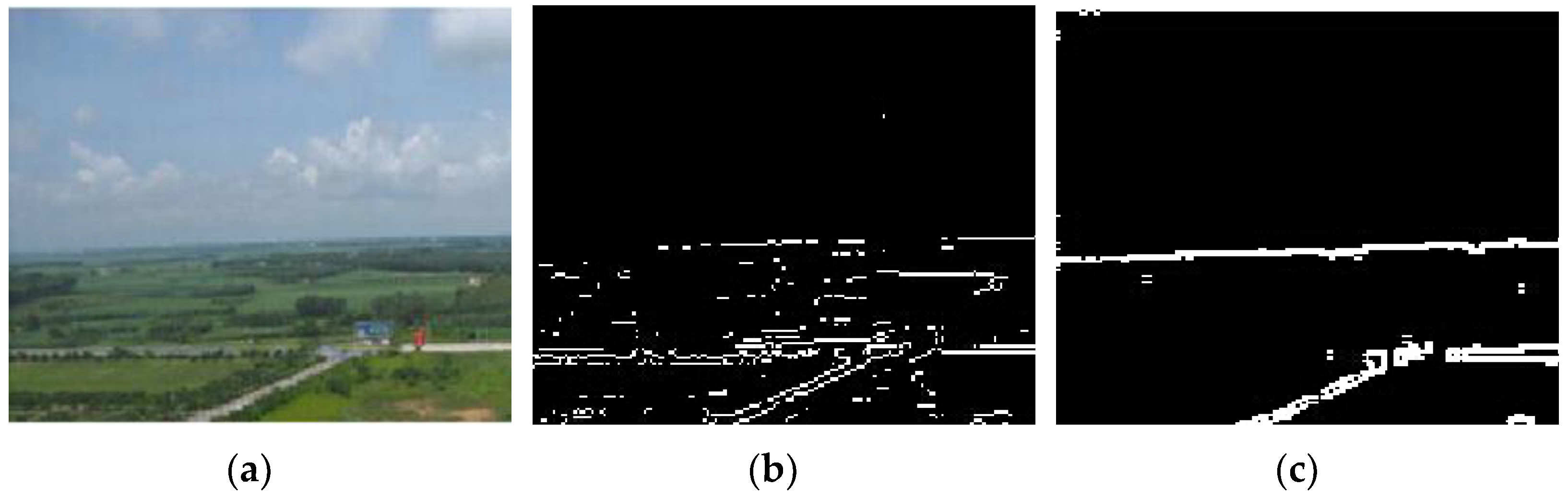
Figure 4 presents a comparative analysis of the edge detection results using the basic and improved versions of the Canny algorithm. The result obtained using the basic Canny algorithm shows blurred edges, missed weak edges, and noticeable noise. In contrast, the improved Canny algorithm produces clearer and more continuous edges while significantly reducing noise. This comparison highlights the advantages of the improved algorithm in terms of edge clarity and noise suppression, validating the effectiveness of the proposed enhancement.

After the edge detection of the image, the image containing the horizon edge is obtained. In order to obtain accurate horizon parameters, it is necessary to extract the line from the image after edge detection. The traditional Hough transform achieves line detection by mapping image edge points to parameter space; nevertheless, it requires traversing all edge points (totaling M), which leads to large computation and high storage costs. Therefore, the progressive probabilistic Hough transform is adopted in this paper to calculate a subset of the edge points (the number is m, and the number is satisfied $m<M$), thus significantly reducing operational complexity and storage requirements [32]. In addition, the method can directly detect the two endpoints of the line, enabling accurate line positioning without relying on post-processing.

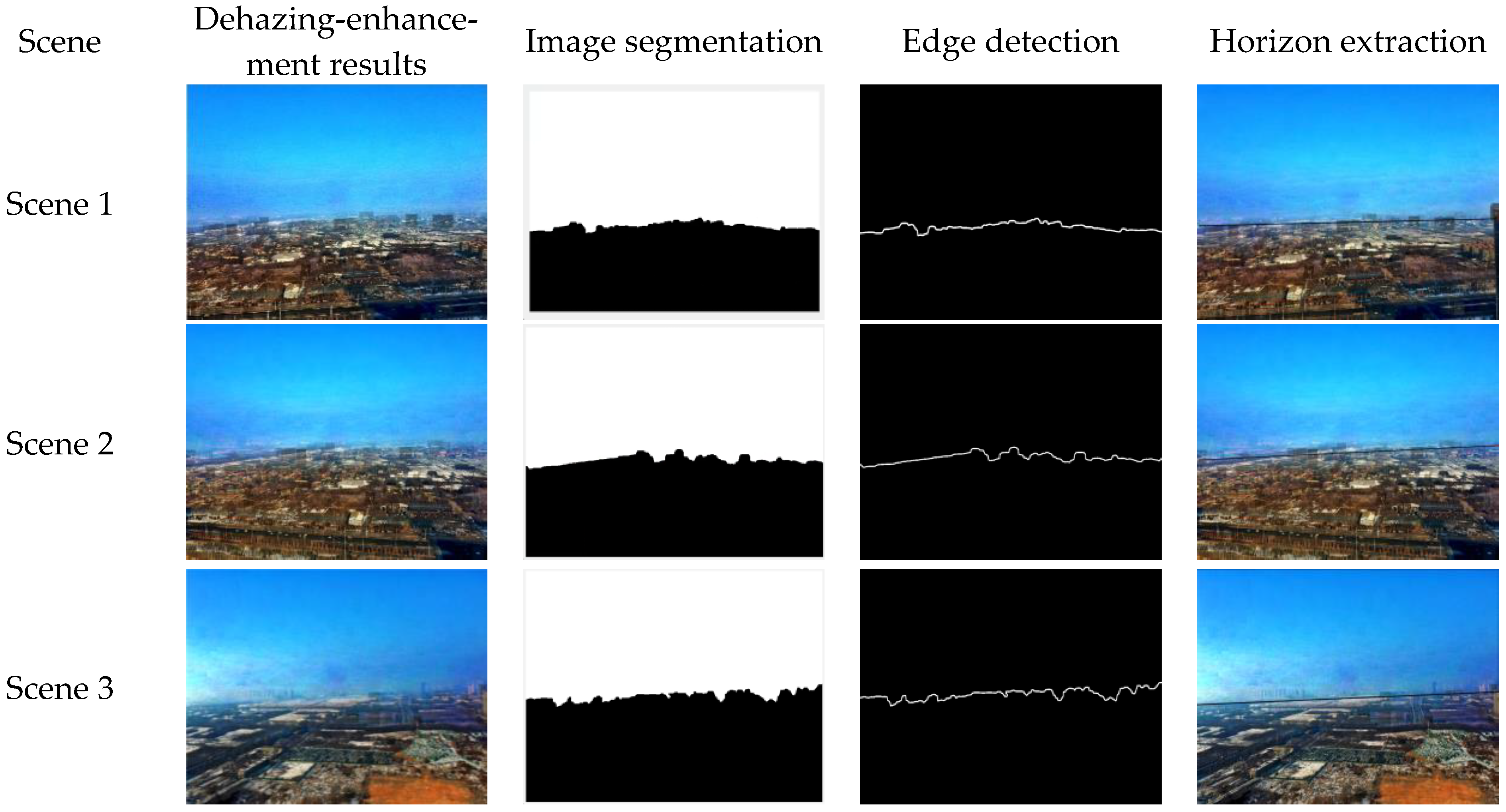
To evaluate the robustness and consistency of the proposed horizon line detection algorithm, Figure 5 presents the processing results for three representative image frames. These frames were selected to include variations in viewpoint and scene composition. As illustrated, the algorithm accurately identifies the horizon line in each case, demonstrating its stable performance across different inputs. This confirms the method’s potential for reliable application in real-world UAV visual attitude estimation tasks.

2.4. Attitude Estimation Algorithm Based on Horizon

According to the horizon projection model shown in Figure 6, the world coordinate system, the body coordinate system and the image coordinate system are established. The camera is fixed on the head of the UAV, with the camera coordinate system overlapped with the body coordinate system.

Let p_w represent any point on the horizon whose coordinate in the world coordinate system is $p_w=\left(x_w,0,0\right)$, then the coordinates of the projection point p’ in the pixel coordinate system can be obtained by the following formula:

$$s{p}_u=AR(R_0{\mathrm{p}}_w+T)$$

(15)

where s is the scale factor, A is the internal reference matrix, and R is the rotation matrix, $R=R_1{R}_2{R}_3$, with R₁, R₂, and R₃ corresponding to the rotation matrices obtained around the three axes, respectively. R₀ denotes the rotation matrix of the UAV at its initial position. Assuming that the center point o_w of the world coordinate system is located on the yoz plane, the position of o_w in the camera coordinate system is $T={\left(0,t_y,t_z\right)}^T$, and the yaw angle is 0. The following expansion of Equation (15) can be obtained:

$$s\left[\begin{array}{c}u\\ v\\ 1\end{array}\right]=\left[\begin{array}{c}{f}_x[x_w\cos \varphi -\sin \varphi (t_y\cos \theta -t_z\sin \theta )]+u_0(t_y\sin \theta +t_z\cos \theta )\\ f_y[x_w\sin \varphi +\cos \varphi \left(t_y\cos \theta -t_z\sin \theta \right)]+v_0(t_y\sin \theta +t_z\cos \theta )\\ t_y\sin \theta +t_z\cos \theta \end{array}\right]$$

(16)

Since the horizon is infinitely distant from the ground, that is, $t_z\to +\infty$, when $\varphi \ne \pi /2$, the variables are brought into the formula and x_w is eliminated. The simplification can be achieved:

$$v=({\displaystyle \frac{f_y}{f_x}}\tan \varphi )(u-u_0)-{\displaystyle \frac{f_y}{\cos \varphi }}\tan \theta +v_0$$

(17)

where f_x, f_y, u_0, and v₀ represent the focal lengths and principal point coordinates in the internal parameter matrix A, respectively. These parameters were obtained via camera calibration, yielding f_x = 417.4831, f_y = 417.5472, u₀ = 327.8796, v₀ = 214.3221. If we assume that the slope of the straight line is k and the intercept is b, then:

$$\left\{\begin{array}{l}\varphi =\arctan (k{\displaystyle \frac{f_x}{f_y}})\\ \theta =\arctan \left[{\displaystyle \frac{(v_0-k{u}_0-b)\cos \varphi }{f_y}}\right]\end{array}\right.$$

(18)

When the roll angle $\varphi =\pm \pi /2$, the horizon in the pixel coordinate system is perpendicular to the u-axis at the point up, then the horizon equation is $u=u_p$ and the pitch angle can be obtained as

$$\theta =\arctan ({\displaystyle \frac{u_p-u_0}{f_x}})$$

(19)

From the above analysis, as long as the horizon in the UAV-captured image can be accurately and reliably extracted, and its linear parameters determined, the roll angle and pitch angles of the UAV can be calculated using the formula.

3. Polarization Orientation Error Compensation Method

Early people found that bees, sand ants, and other animals possess remarkable navigation abilities [33,34]. Subsequent research revealed that these animals use detected sky polarization information to navigate. The skylight polarization forms a macroscopically stable distribution pattern containing rich directional information, including the degree of polarization (DoP) and the angle of polarization (AoP). The polarization degree and the polarization Angle represent the polarization degree of light and the direction of light vibration (E vector direction), respectively. Polarized light can be described by the Stokes vector. The Stokes vector comprises four components, which is $S=[I,Q,U,V]$. I represents the total light intensity. Q and U are two mutually perpendicular linearly polarized components, while V represents circularly polarized light. Given that the sky predominantly exhibits linear polarization, V is typically a value of zero. The formula for calculating the polarization angle and degree is

$$AoLP={\displaystyle \frac{1}{2}}\arctan \left({\displaystyle \frac{U}{Q}}\right)$$

(20)

$$DoLP={\displaystyle \frac{\sqrt{Q^2+U^2}}{I}}$$

(21)

In the polarized light navigation system, the navigation frame and the body frame meet the following conversion relationship:

$$S_b^p=C_n^b{S}_n$$

(22)

where $S_b^p$ is the projection of the solar vector within the body frame, $C_n^b$ is the transfer matrix, and $S_n$ indicates the sun’s position within the navigation frame. When the observed direction aligns with the solar direction, the polarization angle in the body frame can be expressed as

$${\phi }_p^b\left(x_p,y_p\right)={\tan }^{-1}\left(t{\varphi }_s^b\right)$$

(23)

where $(x_p,y_p)$ is the observation point, and ${\varphi }_s^b$ is the solar azimuth in the body frame:

$${\varphi }_s^b={\tan }^{-1}({\displaystyle \frac{S_b^p(2)}{S_b^p(1)}})$$

(24)

The transfer matrix from the navigation frame to the body frame can be expressed as

$$C_n^b=\left[\begin{array}{ccc}\cos \theta \cos \psi & \cos \theta \sin \psi & -\sin \theta \\ \sin \varphi \sin \theta \cos \psi -\cos \varphi \sin \psi & \sin \varphi \sin \theta \sin \psi +\cos \varphi \cos \psi & \sin \varphi \cos \theta \\ \cos \varphi \sin \theta \cos \psi +\sin \varphi \sin \psi & \cos \varphi \sin \theta \sin \psi -\sin \varphi \cos \psi & \cos \varphi \cos \theta \end{array}\right]$$

(25)

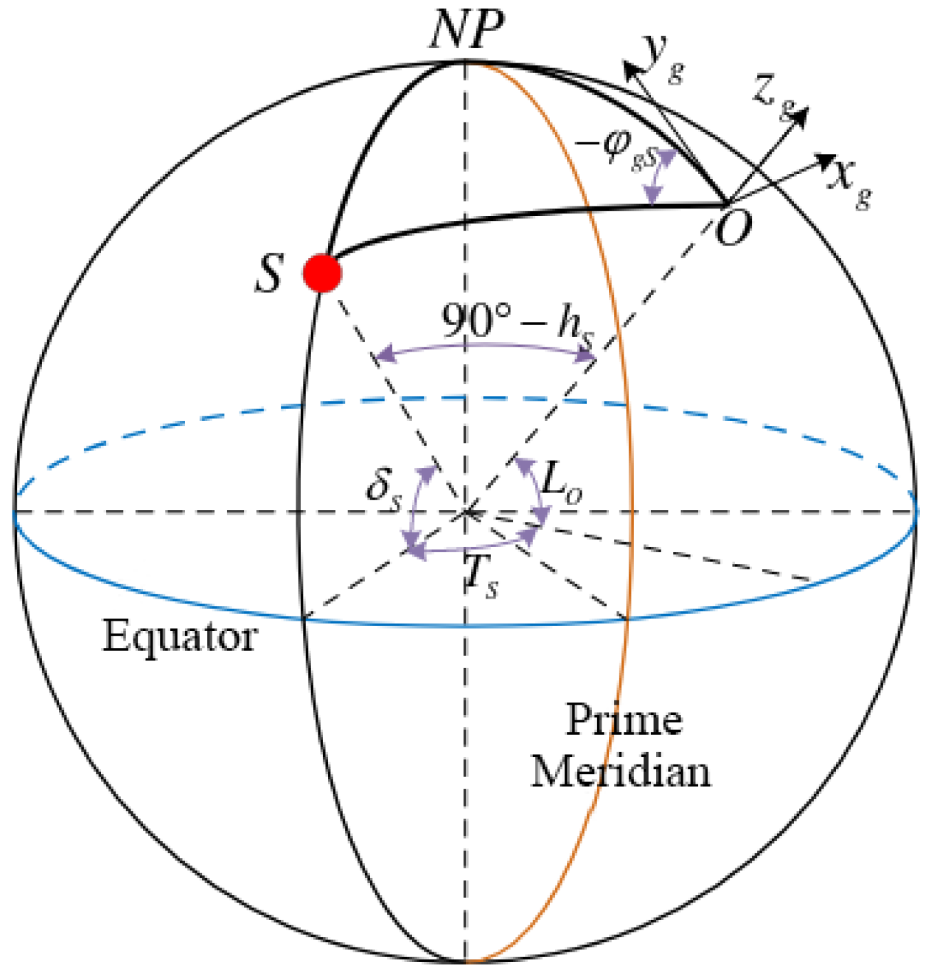
The position of the sun can be solved according to the declination angle of the sun ${\delta }_s$, the solar hour angle $T_S$, and the latitude of the observation site $L_o$, as per the pertinent astronomical theories. By solving the spherical triangle $S-O-NP$ in Figure 7, the sun altitude angle $h_s\in [0^{\circ },{90}^{\circ }]$ and the sun azimuth angle ${\phi }_{gS}\in [0^{\circ },{360}^{\circ }]$ in the east, north, and up (ENU) geographic coordinate system can be obtained.

In Figure 7, the red dot S represents the sun, O represents the observation site, NP represents the North Pole, ${\delta }_s$ signifies the sun’s declination angle, $T_S$ is the sun hour angle, $L_o$ is the latitude of the observation site, $h_s$ is the sun altitude angle, and ${\phi }_{gS}$ is the sun azimuth in the east, north, and up (ENU) geographic coordinate system $o{x}_g{y}_g{z}_g$. The following model can be established in Figure 7:

$$\left\{\begin{array}{l}\sin h_s=\sin {\delta }_s\sin L+\cos {\delta }_s\cos L\cos T_s\\ \cos {\phi }_{gS}={\displaystyle \frac{\sin {\delta }_s-\sin h_s\sin L}{{\cosh }_s\cos L}}\end{array}\right.$$

(26)

To solve the inverse trigonometric function of Equation (26) and perform quadrant judgment, we can obtain the following:

$$h_s=\arcsin \left(\sin {\delta }_s\sin L+\cos {\delta }_s\cos L\cos T_s\right)$$

(27)

$${\phi }_{gS}=\arccos \left({\displaystyle \frac{\sin {\delta }_s-\sin h_s\sin L}{\cos h_s\cos L}}\right)$$

(28)

Among them, the calculation formula of the sun’s declination angle ${\delta }_s$ is as follows:

$$\begin{array}{l}{\delta }_s=0.3723+23.2567\sin {\sigma }_s+0.1149\sin 2{\sigma }_s-0.1712\sin 3{\sigma }_s\\ \hspace{0.33em}\hspace{0.33em}\hspace{0.33em}\hspace{0.33em}-0.758\cos {\sigma }_s+0.3656\cos 2{\sigma }_s+0.0201\cos 3{\sigma }_s\end{array}$$

(29)

where ${\sigma }_s=2\pi (D-D_0)/365.2422$ is the day angle, D is the day of year, and since 1985, the vernal equinox time D₀ expressed in days is

$$D_0=79.6764+0.2422\times \left(Y-1985\right)-\mathrm{INT}\left[\left(Y-1985\right)/4\right]$$

(30)

where Y represents the year and INT represents rounding to zero.

The solar hour angle $T_S$ of the observation site O is calculated as follows, where the local time S_d of the observation site is

$$S_d=S_Z+\left\{F_Z-4\left[120°-\left(Lo{n}_D+Lo{n}_F\right)\right]\right\}/60$$

(31)

where S_Z and F_Z represent the hour and minutes of local Beijing time, whereas Lon_D and Lon_F represent the longitude and latitude.

The calculation formula of the time difference E_t is as follows:

$$E_t=0.0028-1.9857\sin {\sigma }_s+9.9059\sin 2{\sigma }_s-7.0924\cos {\sigma }_s-0.6882\cos 2{\sigma }_s$$

(32)

Using E_t to modify S_d to get true solar time S_t:

$$S_t=S_d+E_t/60$$

(33)

To solve the local solar hour angle $T_S$ according to S_t:

$$T_S=\left(\begin{array}{c}{S}_t-12\end{array}\right)\times {15}^{\circ }$$

(34)

Through the above formulas and solving steps, the solar altitude angle $h_s$ and solar azimuth angle ${\phi }_{gS}$ can be calculated finally. Solar position can be expressed by solar altitude angle and solar azimuth angle as

$$S_n=[\cos h_s\cos {\phi }_{gS},\cos h_s\sin {\phi }_{gS},\sin h_s]$$

(35)

Thus, all remaining variables in Equation (22) have been solved. Substituting the acquired horizontal attitude angle into Equation (22) allows for the compensation of the polarized light heading information.

4. Discussion

4.1. Validation of Horizon Attitude Estimation Algorithm

In order to verify the validity and reliability of the horizon attitude estimation method proposed in this paper, an airborne experiment was carried out with a UAV equipped with a high-resolution camera and a polarization camera. In total, 2278 image frames were collected during the flight for analysis and validation. In addition, the IMU-KVH1750 integrated navigation system, with high-precision fiber/satellite, serves as a reference, offering pitch and roll angle accuracy of 0.015° and heading angle accuracy of 0.035°. The experimental equipment is shown in Figure 8, and the camera parameters are shown in

Table 3. Camera parameters.

Variable	Parameter
Resolution	1280 × 720
Focus distance (mm)	3.24
Sensor format (inch)	1/2.5
Field of view (°)	90

.

This UAV platform was selected due to its stable flight performance and sufficient payload capacity, allowing for the effective integration of the necessary sensors. Furthermore, its ability to execute diverse tilt maneuvers made it well-suited for testing the proposed tilt-induced error compensation method under realistic dynamic conditions. However, one limitation of this platform is its moderate resistance to environmental disturbances, such as wind gusts, which may introduce additional motion noise.

The proposed horizon attitude estimation algorithm in this paper is compared with the following methods: traditional horizon attitude estimation approaches, optical flow-based attitude estimation algorithms, isomorphic matrix attitude estimation methods based on SIFT feature points, and reference data. After the UAV completes its flight mission, the attitude estimation results and error curves for all methods are generated using MATLAB R2020a software. Figure 9 and Figure 10, respectively, display the pitch angle and roll angle estimations obtained by each algorithm. Figure 11 presents the error curves for pitch and roll angles for all compared methods.

The pitch and roll angle attitude estimation results indicate that the isomorphic matrix attitude estimation method based on SIFT feature points exhibits significant systematic bias in both pitch and roll angle calculations, along with pronounced numerical fluctuations. The optical flow-based method displays reduced error fluctuations and superior overall stability compared to the SIFT-based isomorphic matrix approach, though periodic oscillations persist under motion blur interference. The traditional horizon attitude estimation algorithm shows substantial attitude angle deviations at three sampling nodes (609, 1296, and 1668) due to hazy conditions. In contrast, the proposed horizon attitude estimation method achieves optimal accuracy in both pitch and roll angle calculations, with enhanced overall stability, thereby validating the effectiveness of the proposed algorithm.

Table 4. Pitch angle error comparison table of different attitude estimation methods.

Performance Metric	SIFT	Optical Flow	Traditional Horizon	Proposed
RMSE (°)	0.8107	0.4831	0.3957	0.2568
STD (°)	0.7392	0.3704	0.3256	0.2284

and

Table 5. Roll angle error comparison table of different attitude estimation methods.

Performance Metric	SIFT	Optical Flow	Traditional Horizon	Proposed
RMSE (°)	0.7499	0.4390	0.2995	0.2383
STD (°)	0.6739	0.3872	0.2956	0.2366

present a comprehensive performance analysis by detailing the Root Mean Square Error (RMSE) and Standard Deviation (STD) of pitch and roll angle estimation errors for each algorithm. As shown in the tables, the proposed attitude estimation method outperforms the other methods in both error metrics.

4.2. Verification of Polarization Orientation Error Compensation Method

In this experiment, the UAV is equipped with a polarized light sensor to obtain polarized light information at various tilt degrees, aiming to verify the feasibility and accuracy of using a horizontal attitude angle to compensate for the polarized light heading under inclined conditions. The heading data before and after compensation were compared with the real heading data obtained by the high-precision benchmark, and the experimental results are shown in Figure 12 and Figure 13.

Figure 12 illustrates the comparison results between the heading angle of the polarized light and the reference prior to and following compensation. The figure demonstrates how the raw polarized light data exhibit substantial fluctuations and deviation from the reference due to the tilt factor affecting the measurements. This deviation is particularly noticeable at certain sample points, where the angle reaches significant extremes. After compensation, the heading angle of the polarized light aligns more closely with the reference, showing a marked reduction in error. The results clearly highlight that the compensation method substantially reduces the misalignment, confirming the effectiveness of the horizontal attitude angle in correcting heading errors. Figure 13 illustrates the comparison of the heading error in polarized light before and after compensation. The pre-compensation error, represented by the gray dashed line, shows high variability and spikes, which suggests significant inaccuracies in the heading calculation. This is primarily due to the effects of tilt and environmental factors. After compensation (red line), the error is significantly reduced, with a marked decrease in error amplitude and frequency. The post-compensation curve shows a much more stable and smaller range of error, further confirming that the proposed compensation method effectively minimizes heading errors, improving overall heading accuracy.

Table 6. Comparison table of error before and after heading compensation.

Method	RMSE (°)	STD (°)	Mean (°)
pre-compensation	5.0869	5.0633	0.5005
post-compensation	1.1485	1.1441	−0.1039

provides a quantitative comparison of the heading error before and after the application of the compensation method. It lists the root-mean-square error (RMSE), standard deviation (STD), and mean heading error for both the pre-compensation and post-compensation cases. The results show a substantial improvement in all metrics post-compensation: The RMSE decreases from 5.0869° to 1.1485°, a reduction of approximately 77.4%, indicating a significant reduction in the overall heading error. The standard deviation (STD) also decreases, from 5.0633° to 1.1441°, showing that the compensation method not only reduces the average error but also stabilizes the data, making the measurements more consistent. The mean heading error shifts from a positive value of 0.5005° (indicating a slight overestimation) to a negative value of -0.1039°, indicating a slight underestimation post-compensation. This shift suggests that the compensation method helps to bring the heading angle closer to the true value.

5. Conclusions

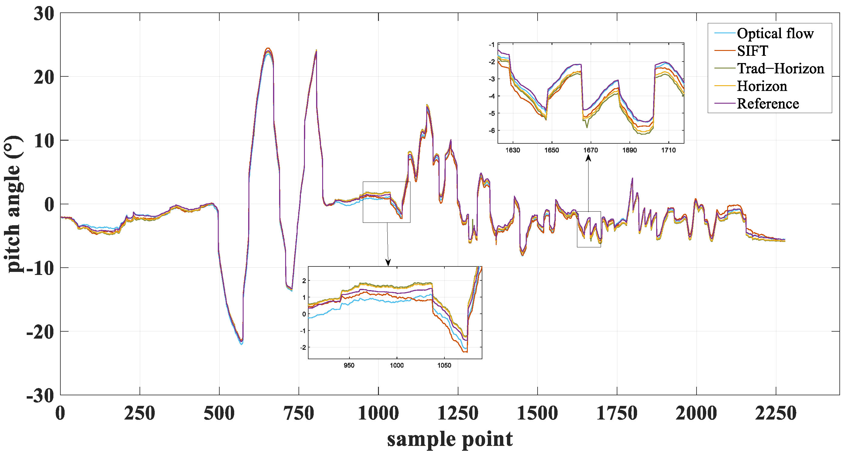
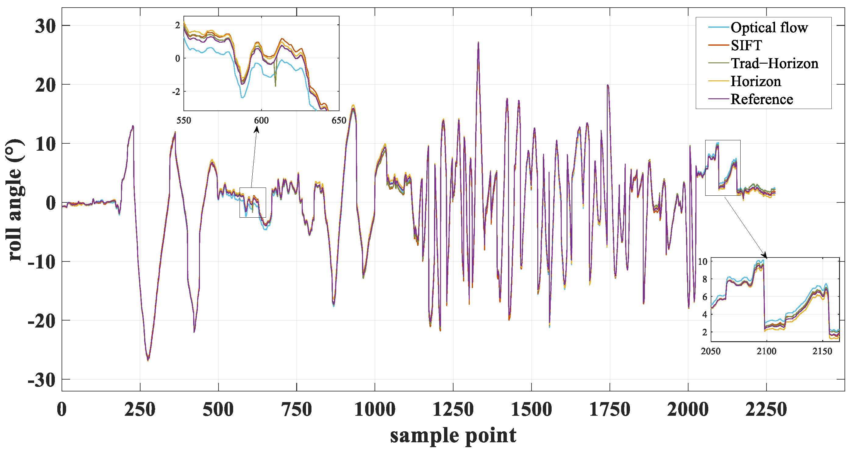
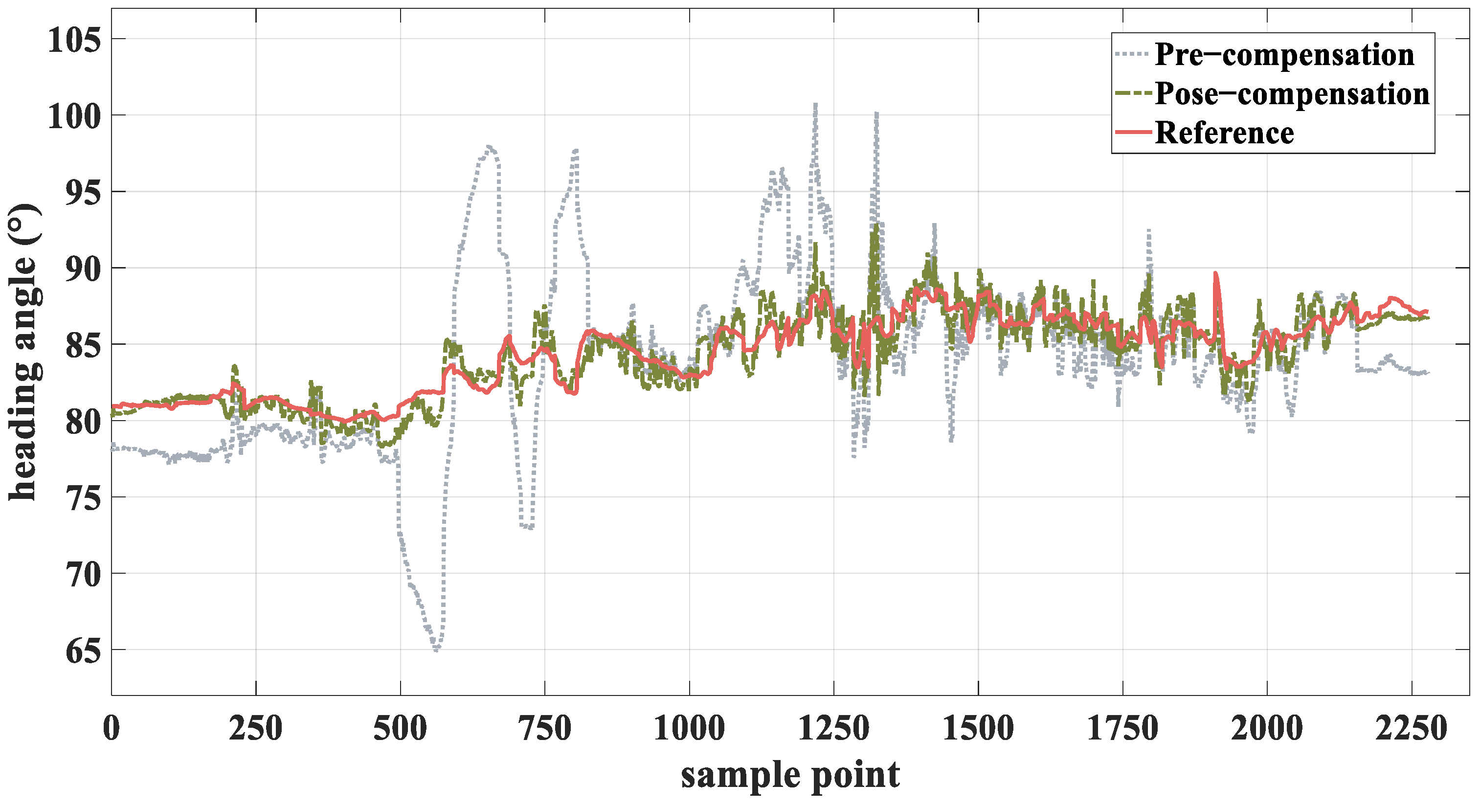
This paper proposes a method to estimate the UAV’s horizontal attitude angle using horizon computation, aiming to compensate for significant heading errors in polarized light navigation under tilted conditions. Firstly, a dehazing-enhancement method integrating Retinex theory and dark channel prior is proposed, improving the algorithm’s adaptability under low illumination and hazy conditions. Secondly, an HSV-based dynamic threshold image segmentation method is developed, significantly enhancing the robustness of horizon extraction. Then, an improved adaptive bilateral filtering Canny operator is employed for edge detection, which not only detects fine edges but also effectively suppresses noise. Finally, the progressive probabilistic Hough transform is employed for line extraction, substantially reducing computational complexity and memory requirements. Subsequent to horizon extraction, the horizontal attitude angle of the UAV is calculated from the horizon parameters. Sensor measurements are converted from the body frame to the navigation frame using coordinate transformation, thereby compensating for polarized light heading errors. Airborne experiments are conducted to validate the efficacy of the suggested method. The experimental results show that the horizontal attitude angle estimation method based on the horizon in this paper has high accuracy. Furthermore, the implementation of the polarization orientation error compensation method proposed in this paper substantially improves the course accuracy and effectively mitigates errors.

While the proposed algorithm achieves high accuracy, it possesses specific limitations. Firstly, in urban or densely forested areas, the horizon is often occluded, causing failure in vision-based horizontal attitude angle estimation. Secondly, horizon detection relies on computationally intensive image processing algorithms, complicating the fulfillment of real-time requirements. Additionally, when the UAV undergoes large roll or pitch angles, errors in the polarized light heading compensation model increase significantly, degrading compensation performance. Future research might involve multi-source sensor fusion for attitude estimation to reduce reliance on single-source visual information while optimizing image processing algorithms to enhance real-time performance. Additionally, the polarized light heading compensation model requires refinement to improve stability under large-angle conditions.