Online Prediction of Concrete Temperature During the Construction of an Arch Dam Based on a Sparrow Search Algorithm–Incremental Support Vector Regression Model

Abstract

The accurate prediction of concrete temperature during arch dam construction is essential for crack prevention. The internal temperature of the poured blocks is influenced by dynamic factors such as material properties, age, heat dissipation conditions, and temperature control measures, which are highly time-varying. Conventional temperature prediction models, which rely on offline data training, struggle to capture these time-varying dynamics, resulting in insufficient prediction accuracy. To overcome these limitations, this study constructed a sparrow search algorithm–incremental support vector regression (SSA-ISVR) model for online concrete temperature prediction. First, the SSA was employed to optimize the penalty and kernel coefficients of the ISVR algorithm, minimizing errors between predicted and measured temperatures to establish a pretrained initial temperature prediction model. Second, untrained samples were dynamically monitored and incorporated using the Karush–Kuhn–Tucker (KKT) conditions to identify unlearned information, prompting model updates. Additionally, redundant samples were removed based on sample similarity and error-driven criteria to enhance training efficiency. Finally, the model’s accuracy and reliability were validated through actual case studies and compared to the LSTM, BP, and ISVR models. The results indicate that the SSA-ISVR model outperforms the aforementioned models, effectively capturing the temperature changes and accurately predicting the variations, with a mean absolute error of 0.14 °C.

1. Introduction

Temperature control and crack prevention in concrete during the construction of arch dams have long been challenging issues in the engineering field [1,2]. Cracks directly impact the load-bearing capacity and durability of the structure, and temperature stress is one of the primary causes of concrete cracking during the construction period [3]. In the actual construction process of arch dams, the pouring block serves as the smallest temperature control unit. Typically, temperature control strategies for each block are formulated based on the monitored temperature within that block. However, concrete temperature is influenced by various time-varying factors, including material properties, age, heat dissipation conditions, and temperature control measures [4,5,6]. Engineers often find it difficult to quantitatively determine temperature control parameters and their effectiveness based on real-time monitoring data, which frequently results in temperature control quality indicators exceeding standards, posing potential risks for concrete cracking. Therefore, constructing a rapid and accurate temperature prediction model and investigating the influence patterns of concrete temperature factors are crucial for crack prevention in dam concrete during construction.

Currently, the methods for predicting the temperature of dam concrete can be broadly categorized into two types: mechanism-driven and data-driven approaches. The former primarily relies on rigorous mathematical derivations and employs numerical methods, such as the finite element method (FEM), to simulate the mechanisms of cement hydration heat release, water pipe cooling, surface heat dissipation, and other factors to obtain the concrete temperature variations over time [7,8,9,10]. This method exhibits strong interpretability, enabling the quantitative analysis of the relationship between various influencing factors and concrete temperature. However, this approach faces bottlenecks such as extensive computational demands and challenges in dynamic parameter calibration under complex scenarios like dam sites [11,12,13], often falling short of meeting the requirements for efficient temperature prediction.

In recent years, advancements in information technology have significantly enriched the empirical data available for data-driven prediction methods. This progress has catalyzed extensive research in dam structural health monitoring, yielding promising outcomes [14,15,16]. In the context of concrete dam temperature prediction, Zhou et al. [17,18,19,20] selected pour temperature, pipe spacing, water flow rate, water temperature, and ambient air temperature at the construction site as input vectors, with the maximum temperature as the output vector, to establish a rapid predictive model for the maximum temperature of concrete in blocks using various neural networks, including a random forest, BP, and the radial basis function. The average mean absolute error ($MAE$) of the predicted results was 0.32 °C. Kang [21] proposed a model incorporating the Java optimizer, the salp swarm algorithm, and the least squares support vector machine to simulate temperature effects in dam health monitoring. Song [22] introduced an interval prediction method for concrete temperature fields based on a hybrid kernel relevance vector machine (HK-RVM) and an improved grasshopper optimization algorithm (IGOA). Li [2] developed a short-term predictive model for concrete during dam construction using ANN, with an average root mean square error ($RMSE$) of 0.15 °C for prediction accuracy.

The instantaneous temperature field of concrete during the construction of arch dams is the result of the combined effects of various dynamic factors, including environmental conditions, cement hydration, and construction techniques. Offline models typically treat these dynamic factors as static, making it difficult for such models to capture the evolving characteristics of the temperature field [23]. In the realm of machine learning, this issue is referred to as concept drift, which describes the phenomenon in which the relationship between the data distribution or the target variable and features changes over time [24,25,26]. This change can lead to a decline in the performance of offline models, as they struggle to adapt to new data patterns [27]. It is worth noting that although the use of an offline update strategy with periodic addition of new samples can partially alleviate the problem of concept drift, the rapidly increasing volume of data may significantly increase the model training time. Moreover, the dominance of historical samples may dilute the current prevailing patterns, potentially obscuring true concept drift signals and reducing prediction accuracy.

To address the limitations of existing studies in concrete temperature prediction, this study aims to develop an online prediction model—SSA-ISVR—by integrating incremental support vector regression (ISVR) with the sparrow search algorithm (SSA) for real-time temperature prediction of concrete during arch dam construction. The proposed method incorporates sample selection, an online learning mechanism, and swarm intelligence optimization techniques, with a focus on addressing the following key issues: (1) improving prediction accuracy, (2) enhancing training efficiency, and (3) enabling adaptive learning of the concrete temperature prediction model. By achieving these objectives, this study seeks to effectively forecast temperature variations in concrete and thereby improve the precision of crack prevention and control during arch dam construction.

Figure 1 illustrates the overall framework of the modeling approach. The structure of this paper is as follows: Section 2 presents the data collection process and the SSA-ISVR modeling method. Section 3 provides a detailed description of the modeling procedures in the case study. Section 4 provides an analysis and discussion of the case study results. Conclusions are drawn in Section 5.

Figure 1. The framework of the online prediction model of concrete temperature for arch dams.

2. Methodology

This section introduces the construction method of the SSA-ISVR model for online concrete temperature prediction. The methodology primarily consists of two parts: data collection and model development. The model’s development includes three key components. First, considering the sensitivity of ISVR performance to hyperparameter settings, the sparrow search algorithm (SSA) is employed to optimize the penalty parameter and kernel coefficient, enhancing prediction accuracy. Second, to ensure the model effectively adapts to changing construction and environmental conditions, the Karush–Kuhn–Tucker (KKT) conditions are introduced to identify previously unseen information [28], which triggers model updates. Moreover, redundant samples are eliminated based on similarity and error-driven criteria to improve training efficiency. This approach enables continuous model adaptation while reducing unnecessary computations. The detailed methodology is described as follows.

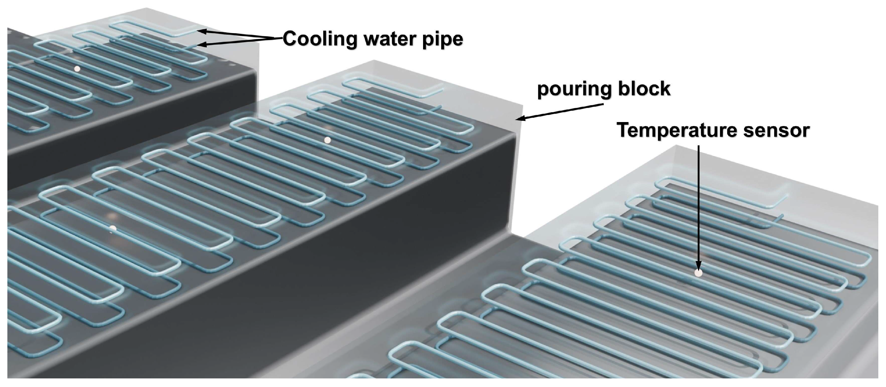
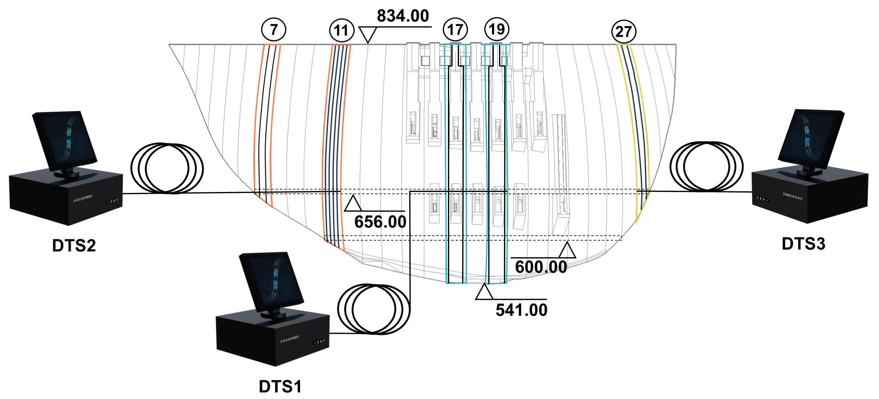
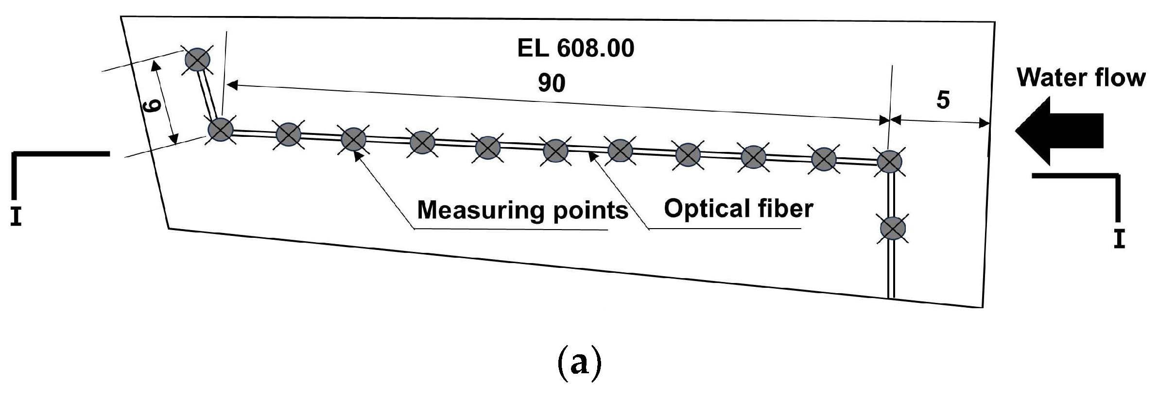
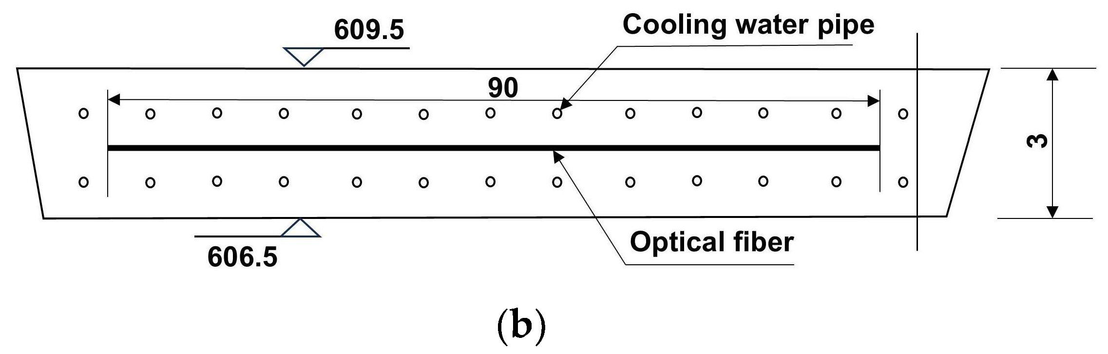
2.1. Data Collection Method

To improve heat dissipation and stress distribution in the dam body, arch dams typically employ a block-segmentation construction technique, dividing the dam along its axis into blocks with lengths of 20–25 m and thicknesses of 1.5–4.5 m. These blocks, as the smallest control units for temperature regulation and crack prevention in concrete dams, are cast in a staggered sequence, resulting in a jagged surface profile between adjacent blocks during dam construction. Firstly, such a construction method leads to varying heat dissipation conditions for the blocks at various stages. Secondly, the interior of the blocks generally contains cooling water pipes, allowing engineers to regulate internal temperatures by adjusting the cooling water’s temperature and flow rate. Additionally, the exothermic process of cement hydration in concrete is also influenced by environmental conditions and construction practices. These time-varying factors result in significant temporal characteristics in the temperature evolution patterns of the pouring blocks. To obtain the temperature of the pouring blocks, engineers typically embed temperature sensors between two layers of cooling water pipes within them to conduct dynamic temperature monitoring. Figure 2 provides a schematic diagram of the arrangement of cooling water pipes and temperature sensors within a block. Several temperature sensors, such as thermocouple temperature sensors, fiber optics, etc., are usually installed in a block, and the frequency of temperature data collection is set according to the size and construction requirements of the dam. Moreover, data such as air temperature and cooling parameters of the water pipes, including water temperature and flow rate, can be obtained according to on-site monitoring and construction records.

Figure 2. Temperature collection within pouring blocks.

2.2. A Concrete Temperature Prediction Model Based on SSA-ISVR

2.2.1. Feature Selection for Model Inputs

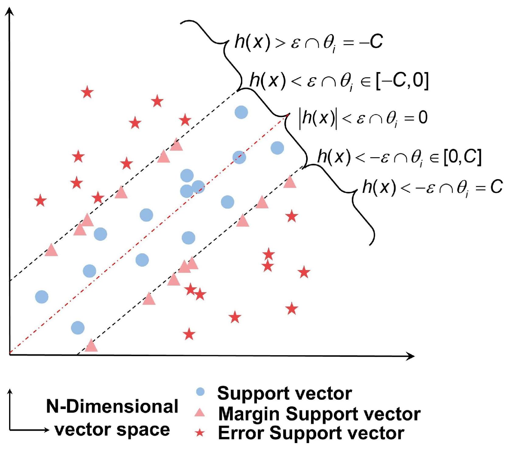
The basis of machine learning predictive models is to construct a system that does not require explicit human-provided features and rules but instead predicts unknown data by learning hidden patterns and rules within the data [29]. Unlike statistical predictive models, machine learning models focus on the data input into the model and the model’s hyperparameters, requiring little to no feature engineering to uncover the relationships between features and targets. Although these relationships often cannot be quantitatively characterized, their accuracy is well recognized.

According to Section 2, the temperature evolution of the blocks is the result of heat generation and transfer. Factors such as the heat of cement hydration, ambient air temperature, water pipe cooling, heat dissipation conditions, and construction practices all influence the block temperature. In summary, this study models the temperature variation process in the casting blocks of a concrete arch dam using a machine learning algorithm (SSA-ISVR), taking into account the multiple influencing factors. Many factors have been validated to exhibit strong correlations with concrete temperature according to long-term research results in the field of concrete temperature control by the authors’ team [2,5,10,12,17,18,19,20,30], primarily including

T = {Concrete age ($A_t$, t), initial temperature ($T_0$, t), ambient temperature ($T_a$, t), cooling inlet water temperature ($T_w$, t), cooling water flow rate ($F_w$, t), heat dissipation area of the block ($C_a$, t), concrete grade ($L_c$, t), height of the block ($H_c$, t), and intermittent time of the block ($R_c$, t)}.

This section may be divided by subheadings. It should provide a concise and precise description of the experimental results, their interpretation, as well as the experimental conclusions that can be drawn.

2.2.2. SVR Theory

It is often challenging to acquire substantial sample data during the early stages of construction. Compared to other models, the support vector regression (SVR) model can construct accurate models with minimal training samples while maintaining insensitivity to outliers. Therefore, this study employed SVR for predictive modeling.

SVR is a regression algorithm based on support vector machines (SVMs), and its core principle involves identifying an optimal hyperplane to partition the data. This hyperplane is used to fit the data points so that all training samples reside within a certain distance, denoted as $\epsilon$ [31], which determines the model’s accuracy and generalization capability. If the difference between a sample’s predicted value and its actual value is less than $\epsilon$, the sample is regarded as correctly predicted. Furthermore, SVR introduces slack variables to allow certain points to violate the $\epsilon$-region constraint, thereby enhancing the model’s robustness. SVR can be formulated as a quadratic programming problem with linear constraints, as shown in Equations (1) and (2):

$$\underset{w,b,{\xi }_i,{\widehat{\xi }}_i}{\min }={\displaystyle \frac{1}{2}}{‖w‖}^2+C{\displaystyle \sum _{i=1}^m\left({\xi }_i,{\widehat{\xi }}_i\right)}$$

(1)

$$s.t.\left\{\begin{array}{l}f\left(x_i\right)-y_i\le \epsilon +{\xi }_i\\ y_i-f\left(x_i\right)\le \epsilon +{\widehat{\xi }}_i\\ {\xi }_i\ge 0,{\widehat{\xi }}_i\ge 0,i=1,2,\cdots ,m\end{array}\right.$$

(2)

Using the Lagrange multiplier method, the constraints in Equation (1) can be transformed into equality conditions, and a kernel function is introduced to represent the mapping from a lower-dimensional space to a higher one. This ultimately converts the linearly constrained quadratic programming problem into a dual optimization problem [32], as depicted in Equations (3) and (4):

$$\underset{a,a^{*}}{\min }={\displaystyle \frac{1}{2}}{\displaystyle \sum _{i=1}^n{\displaystyle \sum _{j=1}^n{Q}_{ij}(a_i-a_j*)(a_j-a_j*)+{\displaystyle \sum _{i=1}^n\epsilon (a_i+a_i*)}}}-{\displaystyle \sum _{i=1}^n{y}_i(a_i-a_i*)}$$

(3)

$$s.t.0\le a_i,a_i^{*}\le C,{\displaystyle \sum _{i=1}^n(a_i-a_i^{*})=0,i=1,\dots ,n}$$

(4)

Since the objective function of the dual optimization is convex, it ensures that a global optimal solution can be found. Additionally, by employing various kernel functions (such as linear kernels, polynomial kernels, and radial basis function kernels), the data can be mapped to a higher-dimensional space, facilitating the identification of linear relationships in this space, which is particularly useful for handling nonlinear regression problems. Moreover, SVR exhibits some tolerance to noise, as it defines parameters like allowable error and slack variables, making the model insensitive to small errors. Consequently, SVR is highly suitable for the requirements of the temperature prediction of pouring blocks with significant time-varying characteristics.

2.2.3. SSA Optimization Algorithm Theory

Additionally, the SVR model’s performance largely depends on the training samples and model parameters. To achieve more accurate results, the SSA optimization algorithm was utilized for the selection of SVR parameters.

The SSA [33] is an emerging swarm intelligence optimization algorithm proposed by Xue et al. in 2020. This algorithm simulates sparrows’ foraging and anti-predation behaviors to update and optimize their positions. Compared to other optimization algorithms, SSA features a simple structure, fast convergence speed, and outstanding performance in escaping local optima [34]. It only requires the configuration of basic parameters such as population size and maximum iterations, thereby reducing the workload of parameter tuning and enhancing the algorithm’s applicability and stability.

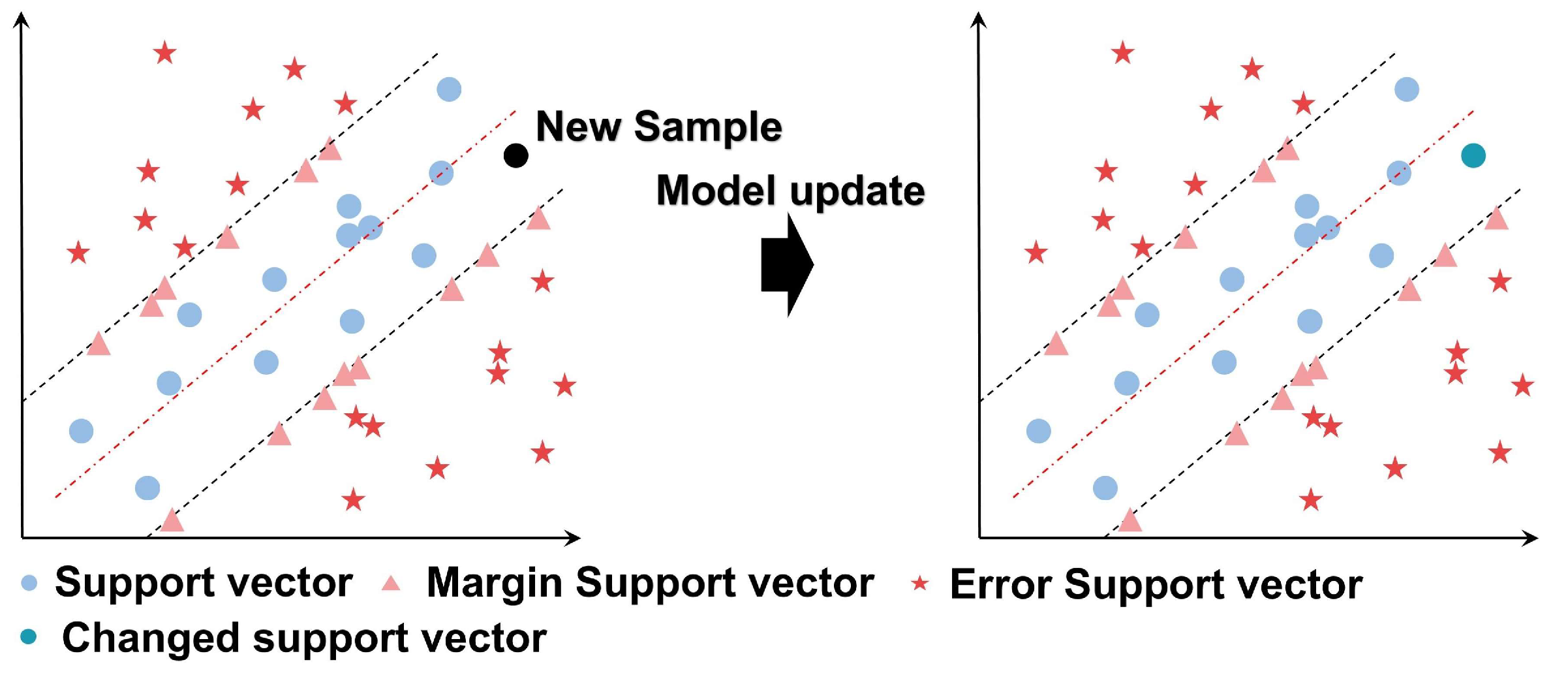
2.3. Sample Augmentation and Reduction Methods

As new monitoring samples accumulate, simply incorporating all new samples into incremental learning models can degrade training efficiency and even hinder the accurate capture of dynamic temperature variations in concrete. Given this, implementing a dynamic sample selection mechanism is essential for online learning. To efficiently adapt the model to the changes in construction and environmental conditions, it is necessary to precisely identify the unlearned information in samples and promptly include it in the training sample set. Meanwhile, considering the rapid growth of sample size, redundant samples should be removed in a timely manner. The specific sample selection methods will be elaborated below.

2.3.1. KKT Condition Examination for New Samples

In the optimization framework of support vector regression (SVR), the KKT conditions serve as both sufficient and necessary conditions for convex optimization problems [35]. Examining whether the Lagrange multipliers are zero can determine whether samples are support vectors, thereby identifying under-learned sample information in the SVR model. This provides a basis for sample updates in incremental learning [36].

For the optimal solution $a=\left[a_1,a_2,\cdots ,a_i\right]$ in the dual problem discussed in Section 3.1, each sample satisfies the KKT conditions for the optimal solution of the optimization problem:

$$\left\{\begin{array}{l}E=\{i\left|\left|{\theta }_i\right|=\right.C,\left|h(x_i)\right|>\epsilon \}\\ S=\{i\left|0<\left|{\theta }_i\right|<C,\left|h(x_i)\right|\right.=\epsilon \}\\ R=\left\{i\left|{\theta }_i=0,\left|h(x_i)\right|<\epsilon \right.\right\}\end{array}\right.$$

(5)

Based on the model, the error of the sample coefficient can be defined as ${\theta }_i=a_i-a_i^{*}$, and the boundary function is denoted as $h(x_i)=f(x_i)-y_i$. In this context, samples in set $\left|{\theta }_i\right|=C$ are distributed outside the $\epsilon$-region, while samples in set $0<\left|{\theta }_i\right|<C$ lie on the boundary of $\epsilon$, and samples in set $\left|{\theta }_i\right|=0$ are distributed inside the $\epsilon$-region.

Figure 3 illustrates the sample set division, where the error support vector is in set $E$, the margin support vector is in set $S$, and the support vector is in set $R$.

Figure 3. Sample set division. Black dashed lines represent the supporting hyperplanes, while red dashed lines denote the optimal separating hyperplane.

If $\{x_{new},y_{new}\}$ represents a new sample, its KKT condition can be expressed as either $\left|h(x_{new})\right|>\epsilon$ or $\left|h(x_{new})\right|<\epsilon$. When $\left|h(x_{new})\right|>\epsilon$, it indicates that the new sample does not satisfy the KKT conditions (as shown in Figure 4), suggesting that the original support vectors do not contain this information and that the model’s prediction error is significant. Therefore, it is necessary to learn from the new sample. Conversely, when $\left|h(x_{new})\right|<\epsilon$, it implies that the new sample satisfies the KKT conditions (as shown in Figure 5), indicating that the information is already included in the current support vectors, and thus, the new sample can be discarded.

Figure 4. The new sample violates the KKT conditions.

Figure 5. The new sample meets the KKT conditions.

2.3.2. Selective Elimination Strategy Based on Sample Similarity

In online learning, the most common approach to handle redundant samples is to employ a sliding window to discard the oldest samples. However, the evolution of concrete temperature is closely related to its prior thermal history, meaning older samples may not entirely lose their representation of current temperature characteristics. Therefore, this study introduces Euclidean and cosine distances to accurately quantify the differences between samples to compute inter-sample similarity [37,38,39]. The similarity reflects the degree of divergence between the sample information. That is, a higher similarity indicates smaller informational differences between samples. The similarity is calculated as follows:

$$S_i=\beta d(x_i,x_{new})+\left(1-\beta \right)\cos \theta (x_i,x_{new})$$

(6)

$$\left\{\begin{array}{l}d(x_i,x_{new})={‖{\displaystyle \frac{x_i-x_{new}}{S}}‖}_2\\ \cos \theta (x_i,x_{new})=\mathrm{arc}\cos \theta ({\displaystyle \frac{x_i^T{x}_{new}}{{‖x_i‖}_2\cdot {‖x_{new}‖}_2}})\end{array}\right.$$

(7)

where $\beta$ is the coefficient, $d(x_i,x_{new})$ is the Euclidean distance, $\cos \theta (x_i,x_{new})$ is the cosine similarity, and $x_{new}$ is the new sample.

When the inclusion of new samples exceeds the maximum storage capacity, Equations (6) and (7) are employed to calculate the similarity between existing and new samples, after which the existing sample showing the lowest similarity to the latest samples is eliminated.

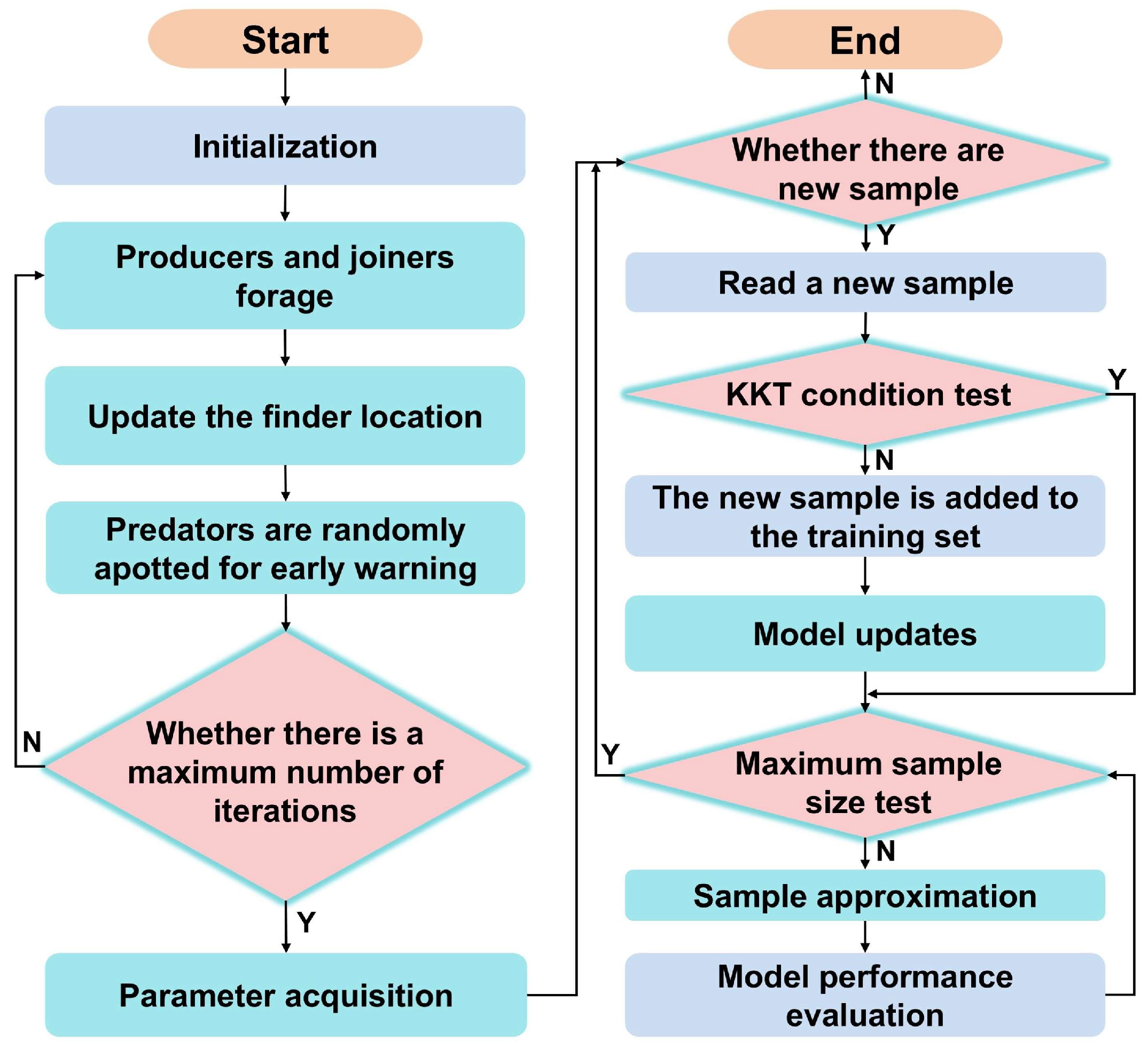
2.4. Online Modeling Method for Temperature Prediction in Arch Dams Based on SSA-ISVR

The online modeling process used in this study is as follows:

Step 1: Data Collection and Preprocessing: this step primarily involves handling missing and abnormal values by using methods such as nearest neighbor imputation and sample screening.

Step 2: this step includes setting different parameter ranges for the SSA, pretraining the ISVR model, and determining the initial SSA-ISVR model parameters to obtain a reliable teacher model.

Step 3: Sequentially acquire new samples, perform the KKT condition test, update the model, and evaluate model performance. Sequentially acquired new samples are inputted through the KKT condition test, based on which the model is updated accordingly. Then, the model’s performance is evaluated.

Step 4: The number of samples is checked to determine whether it exceeds the maximum capacity. If the number surpasses this threshold, a reduction is carried out based on the similarity of the samples and an error-driven analysis.

Step 5: the prediction results are generated, and the model error is evaluated.

This modeling process is illustrated in the flowchart in Figure 6.

Figure 6. Online modeling process. Y stands for Yes and N stands for No.

3. Case Study

3.1. Project Overview

This section focuses on a specific arch dam, which was a concrete double-curvature arch dam consisting of 31 segments. The dam had a maximum height of 289 m, a crest arc length of 709 m, a crest thickness of 14 m, a maximum arch-end thickness of 83.91 m, and a maximum thickness of 95 m, including the expanded foundation. The total concrete volume was approximately 8 million m³. The construction of the dam did not include longitudinal joints; instead, it employed a monolithic casting method with large concrete volumes and high construction continuity, which considerably increased the difficulty of temperature control during construction. Additionally, the dam is located in the subtropical monsoon region, where the average annual temperature is 21.95 °C. The average temperature in January, the coldest month, is 12.4 °C, while in July, the hottest month, the temperature reaches 26.5 °C, with extreme temperatures ranging from a maximum of 42.7 °C to a minimum of −0.3 °C. The climatic conditions are characterized by distinct wet and dry seasons, strong sunlight, dry winters, hot and rainy summers, and sharp temperature fluctuations, all of which further complicate concrete temperature management. Therefore, both the dam’s specifications and the environmental conditions presented significant challenges for controlling the concrete temperature.

For temperature monitoring, the dam employed distributed fiber optic temperature sensing (DTS) to collect real-time internal temperature data from typical dam segments and special locations, including segments 17 and 19 on the riverbed, segments 7 and 27 on the abutments, and segment 11 as a transition section.

In this study, the fiber-optic temperature sensor was calibrated using constant-temperature water baths. The temperature resolution of the fiber-optic temperature measurement system is 0.05 °C, with a measurement accuracy of 0.1 °C and a spatial resolution of 1.02 m, ensuring reliable monitoring with high resolution across the entire measurement range [40].

Figure 7 shows the layout of the fiber optics within the dam segments and the distribution of the DTS temperature monitoring units.

Figure 7. Distribution of fiber burial locations. Numbers in circles dam section numbers. Lines in different colors denote optical fibers connected to different DTS hosts.

Figure 8a illustrates the arrangement of the fiber optics on the surface of a block, and Figure 8b the cross-sectional view along line I-I.

Figure 8. Fiber embedding scheme: (a) fiber embedding method in 11-008; (b) cross-sectional view on I-I.

3.2. Modeling Preparation

Based on the input feature variables identified in Section 2.2.1, the dataset needs to cover various scenarios, such as multiple strength grades of concrete, different pouring seasons, and various temperature control strategies, to ensure the model’s generalization ability [41,42,43,44,45]. Dam section 7 is in the abutment area, while sections 11 and 17 are in the central region. A dataset comprising 36 blocks from these sections was selected to develop the concrete temperature prediction model. These blocks included different materials (C40, C35, and C30 cement), seasonal variations in pouring time throughout the year (hot season from September to October and cold season from December to January), dynamic temperature control strategies (cooling water temperatures of 10–12 °C and 14–16 °C in the hot and cold seasons, respectively), and seasonal maintenance measures (thicker insulation in the cold season, spray moisturization, and water flow conservation in the hot season).

The temperature data were preprocessed to construct a time-series database with a sampling interval of 0.5 days, covering the entire cooling period (0–120 days). Of the 8640 data points processed, missing values and outliers accounted for about 0.05% of the total data.

Data from 28 pouring blocks were randomly selected as the model’s training set, while the remaining 8 were designated as the test set (ratio of about 8:2). Table 1 shows the statistical properties of the different feature variables of the dataset, which ensures the consistency of the statistical properties among them.

Table 1. Statistics of the dataset.

Input	Statistics
	Training Datasets			Test Datasets
	Average Value	Standard Deviation	Median	Average Value	Standard Deviation	Median
Concrete age (d)	59.75	34.64	59.75	59.72	34.63	59.50
Initial temperature (°C)	20.85	1.96	20.90	20.77	2.02	20.90
Cooling inlet water temperature (°C)	14.60	5.46	14.35	14.10	5.62	13.94
Cooling water flow rate (L/min)	6.24	8.85	6.13	6.36	8.88	6.41
Ambient temperature (°C)	22.97	5.87	23.27	22.93	5.89	23.25
Concrete grade	36.66	2.68	35.00	36.94	2.70	35.00
Height of the block (m)	2.95	0.26	3.00	3.01	0.55	3.00
Intermittent time of the block (d)	13.02	5.73	12.35	12.54	5.40	12.10
Heat dissipation area of the block (m2)	254.59	521.36	0.00	239.87	502.47	0.00

During the modeling process, sample data were normalized between 0 and 1, and the output results were denormalized.

Data preparation was carried out using a database, and model construction and prediction were performed in Python 3.11.0. The computational core used for this study was an R5-5600H CPU at 3.3 GHz with 16 GB of RAM.

Previous studies have demonstrated that the radial basis function (RBF) kernel is one of the most commonly used and widely validated kernel functions for modeling nonlinear data with small sample sizes [46,47]. During the model training process, the RBF kernel provided a favorable balance between computational efficiency and prediction accuracy. Therefore, the RBF kernel function was chosen.

The ISVR model’s hyperparameter ranges were determined as c ∈ [1, 20] and γ ∈ [0.01, 10] based on similar works and multiple tests in this study [48]. The hyperparameters c and γ of the ISVR model were optimized using SSA. The SSA fitness function is the mean absolute error (MAE) between the predicted and measured values. The control parameters include the population size (pop) and the maximum number of iterations (mit), which are set to pop = 100 and mit = 20, respectively. The SSA is designed to be robust and efficient, and the maximum number of iterations is set to c and γ. The final optimized values of c and γ in the initial model were set to 4.722 and 0.062, respectively.

In the online update of the model, the KKT condition was configured with a sample size limit of 1000 and a prediction error threshold of 0.5 °C for new samples to balance computational efficiency and accuracy.

Table 2 compares the impact of different values of the similarity weighting coefficient $\beta$ on the model’s prediction accuracy.

Table 2. Prediction accuracy for various values of the weight coefficient.

Item	β = 0	β = 0.1	β = 0.2	β = 0.3	β = 0.4	β = 0.5	β = 0.6	β = 0.7	β = 0.8	β = 0.9	β = 1
RMSE	0.263	0.262	0.263	0.28	0.269	0.269	0.27	0.272	0.269	0.275	0.27
MAE	0.176	0.174	0.175	0.183	0.179	0.178	0.178	0.181	0.178	0.182	0.186

Comparing the sensitivity of multiple $\beta$ values within the range of 0–1 to the model’s performance, the model showed the optimal accuracy when $\beta$ was 0.1. Therefore, in this article, $\beta$ was set to 0.1.

During the KKT condition test, the time required for a single test was approximately 1 s, while the average time for the model update computation was approximately 48 s.

Additionally, the ISVR, BP, and LSTM models were introduced for performance comparison. Two comparison strategies were employed: (1) comparing the unoptimized BP, LSTM, and ISVR models and (2) comparing the unoptimized ISVR model with the SSA-ISVR model optimized via SSA. The BP and LSTM models utilized well-established modeling mechanisms, where network weights were automatically optimized and can obtain relatively optimal parameters during training through backpropagation. ISVR and BP hyperparameter tuning were performed through cross-validation, while the LSTM model was determined using an early stopping strategy.

All model configurations and training parameters are summarized in Table 3.

Table 3. Model architectures and training parameters.

Model	Hidden Layers	Neurons/Units	Activation Function	Optimizer	Learning Rate	Iterations/Epochs	Other Settings
BP	1	100	Hyperbolic tangent function (Tanh)	Adam	0.01	1000	Training function: Levenberg–Marquardt; early stopping: error < 1 × 10−4 or validation fail > 20
LSTM	1 (LSTM layer)	200	Rectified linear unit (ReLU)	Adam	0.01 (initial)	100	Input steps: 5; output steps: 1; regularization: 0.01; LR decay every 30 epochs by 0.2
ISVR	–	–	RBF kernel	–	–	–	c and γ via grid search: c ∈ [1, 20] and γ ∈ [0.01, 10]; 5-fold CV
SSA-ISVR	–	–	RBF kernel	SSA	–	20 (SSA iterations)	c ∈ [1, 20] and γ ∈ [0.01, 10]; population size: 100; fitness: CV MAE

“– “ indicates none. “Neurons/Units” refers to the number of neurons in the hidden layer (BP) or LSTM units. The ISVR and SSA-ISVR models use support vector regression with radial basis function (RBF) kernels. CV means cross-validation.

3.3. Evaluation Metrics

This study evaluated the model performance using $RMSE$, $MAE$, and the regression coefficient ($R^2$). The calculation formula is as follows:

$$RMSE=\sqrt{{\displaystyle \frac{1}{m}}\ast {\displaystyle \sum _{i=1}^m{(y^{(i)}-{\widehat{y}}^{(i)})}^2}}$$

(8)

$$MAE={\displaystyle \frac{1}{m}}\ast {\displaystyle \sum _{i=1}^m\left|y^{(i)}-{\widehat{y}}^{(i)}\right|}$$

(9)

$$R^2=1-{\displaystyle \frac{{\displaystyle \sum _{i=1}^m{(y^{(i)}-{\widehat{y}}^{(i)})}^2}}{{\displaystyle \sum _{i=1}^m{(y^{(i)}-\overline{y})}^2}}}$$

(10)

where $m$ is the number of samples and $i=1,2,3,\dots ,m$.

4. Results and Discussion

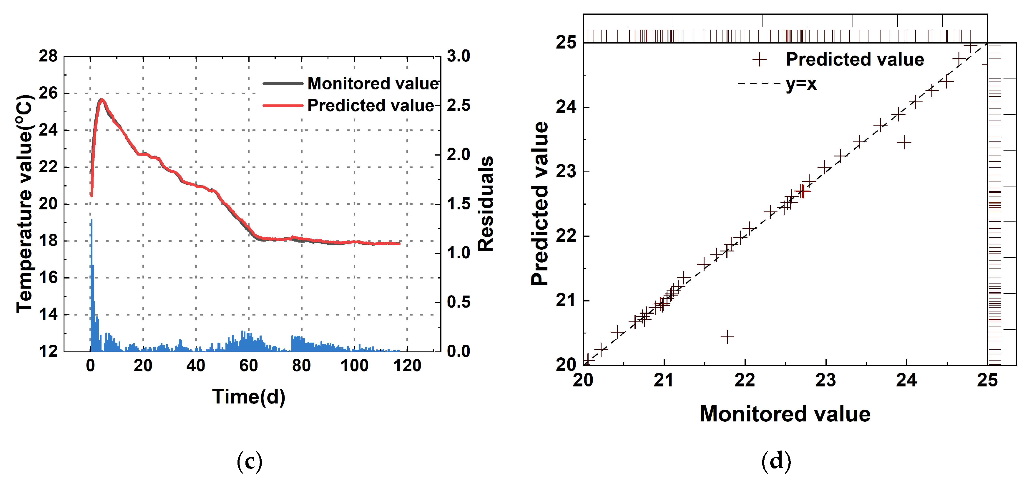
4.1. SSA-ISVR-Based Prediction Results

Based on the online predictions, the temperature prediction evaluation metrics, including $RMSE$, $MAE$, and $R^2$, for multiple blocks were obtained, as shown in Table 4. Figure 9, Figure 10 and Figure 11 illustrate the predicted concrete temperatures for blocks 7, 11, and 17.

Table 4. Evaluation of SSA-ISVR.

Monitoring Point	Offline Training Samples			Online Testing Samples
	RMSE	MAE	R2	RMSE	MAE	R2
7#-026	0.175	0.082	0.996	0.123	0.077	0.996
7#-030	0.155	0.093	0.998	0.112	0.065	0.987
11#-001	0.217	0.104	0.990	0.221	0.139	0.989
11#-012	0.213	0.099	0.989	0.184	0.112	0.995
17#-078	0.195	0.082	0.992	0.170	0.100	0.995
17#-079	0.183	0.071	0.997	0.221	0.090	0.991

Figure 9. Monitoring point in 7: (a) temperature of 7#-026; (b) the regression results of the SSA-ISVR model in 7#-026; (c) temperature of 7#-030; (d) the regression results of the SSA-ISVR model in 7#-030. In subfigures (b,d), color gradient: yellow = high data density, red = Medium density, black = low density, the same below.

Figure 10. Monitoring point in 11: (a) temperature of 11#-001; (b) the regression results of the SSA-ISVR model in 11#-001; (c) temperature of 11#-012; (d) the regression results of the SSA-ISVR model in 11#-012.

Figure 11. Monitoring point in 17: (a) temperature of 17#-078; (b) the regression results of the SSA-ISVR model in 17#-078; (c) temperature of 17#-079; (d) the regression results of the SSA-ISVR model in 17#-079.

From the perspective of the overall model performance, SSA-ISVR achieved excellent predictive accuracy. As shown in Table 2 and Figure 9, Figure 10 and Figure 11, during the pre-training phase, the model yielded an average $RMSE$ of 0.189, an average $MAE$ of 0.08 °C, and an average $R^2$ of 0.994. During the prediction phase, the average evaluation metrics across multiple pouring blocks for SSA-ISVR were $R^2$ = 0.992, $RMSE$ = 0.172, and $MAE$ = 0.097 °C.

In the temperature prediction for a single concrete pour, the prediction error of the SSA-ISVR model (see Figure 9, Figure 10 and Figure 11) was more pronounced during the rapid temperature change phase of the concrete. This was due to the highly exothermic hydration during the early stage of cement. Furthermore, the hydration process was influenced by various construction conditions (such as ambient temperature and temperature control measures), which exacerbated the dynamic temperature variations, causing more prediction errors in contrast to the more stable temperature change phase.

In summary, despite these challenges, the predictive accuracy of SSA-ISVR remains sufficient to meet the requirements of specific engineering applications.

4.2. Comparative Analysis of Different Models

To comprehensively evaluate the performance of the proposed model, this section first analyzes the prediction results presented in Section 4.1, focusing on two aspects: the stability of prediction performance and the prediction errors during different cooling phases. Additionally, an expanded dataset beyond the original training and testing sets was introduced for further validation. This additional dataset covered various system conditions, aiming to extensively assess the generalization and adaptability of the proposed model.

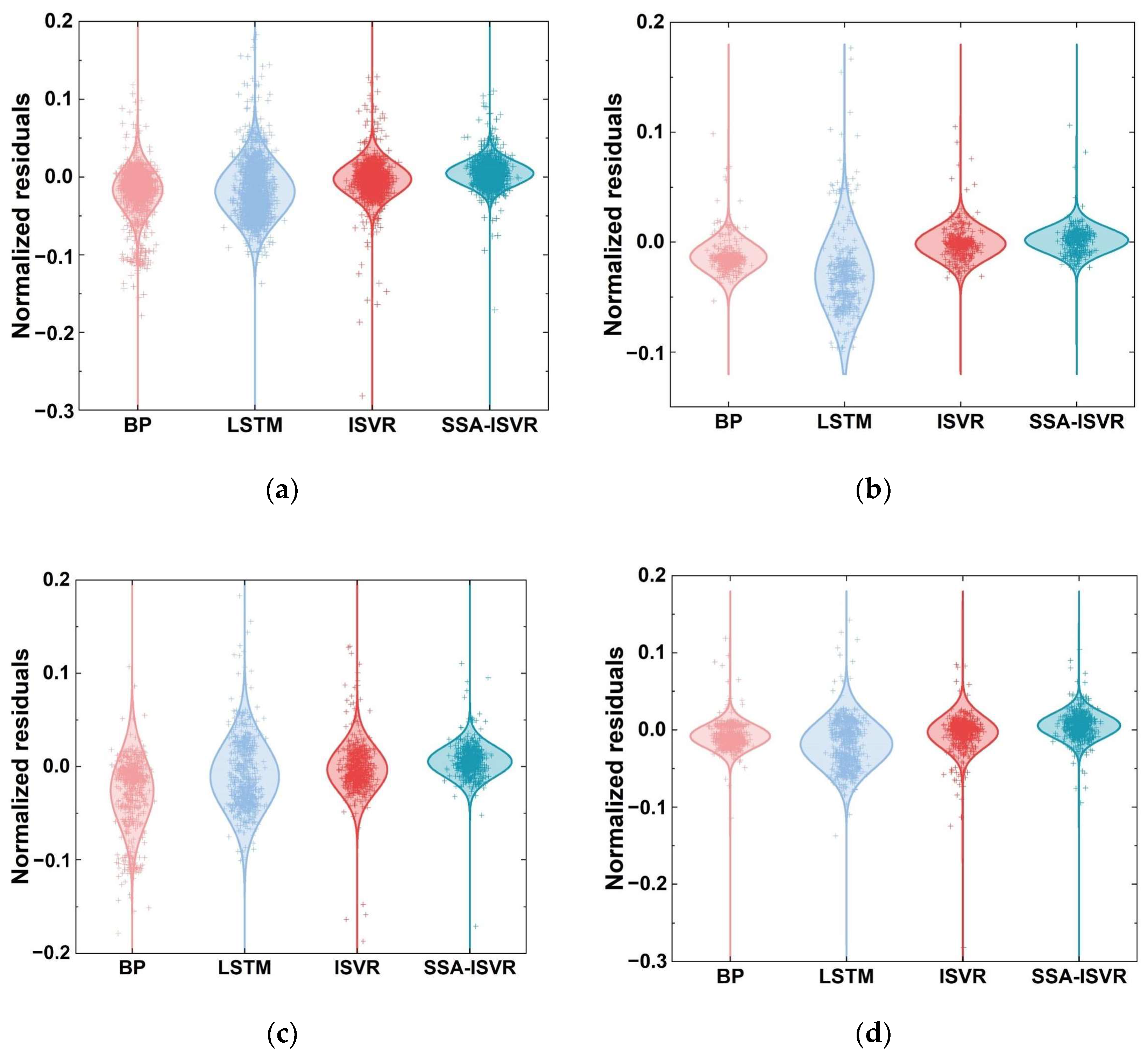
4.2.1. Stability of Prediction Performance

Based on the analysis in Section 4.1, the model exhibited relatively large errors during the 0–21-day period. To further analyze the prediction accuracy of the model, this study compares the performance of the BP, LSTM, ISVR, and SSA-ISVR models in modeling the concrete temperature of several pouring blocks. Table 5 and Figure 12 present the mean and standard deviation of prediction errors for each model.

Table 5. Statistical values of absolute prediction errors.

Statistical Value	Models	Total Test Set	Monitoring Point in 7	Monitoring Point in 11	Monitoring Point in 17
Mean	BP	0.016	0.013	0.026	0.008
	LSTM	0.019	0.031	0.011	0.018
	ISVR	0.005	0.002	0.003	0.004
	SSA-ISVR	0.003	0.002	0.005	0.004
Standard deviation	BP	0.026	0.014	0.036	0.016
	LSTM	0.036	0.036	0.037	0.031
	ISVR	0.021	0.014	0.025	0.021
	SSA-ISVR	0.015	0.012	0.016	0.016

Figure 12. Error distribution of different algorithms: (a) error distribution of the entire test set; (b) error distribution for the monitoring point in 7; (c) error distribution for the monitoring point in 11; (d) error distribution for the monitoring point in 17.

Figure 12 presents the residual statistics and symmetrical normal distribution curves for various concrete temperature prediction models across the entire test set and specific blocks, including segments 7, 11, and 17.

As shown in Table 5 and Figure 12, SSA-ISVR consistently yields the lowest mean absolute error, approximately 0.003, with a standard deviation around 0.014, outperforming the other models. This indicates that SSA-ISVR exhibits lower prediction errors and more concentrated error distribution during the 0–21-day period.

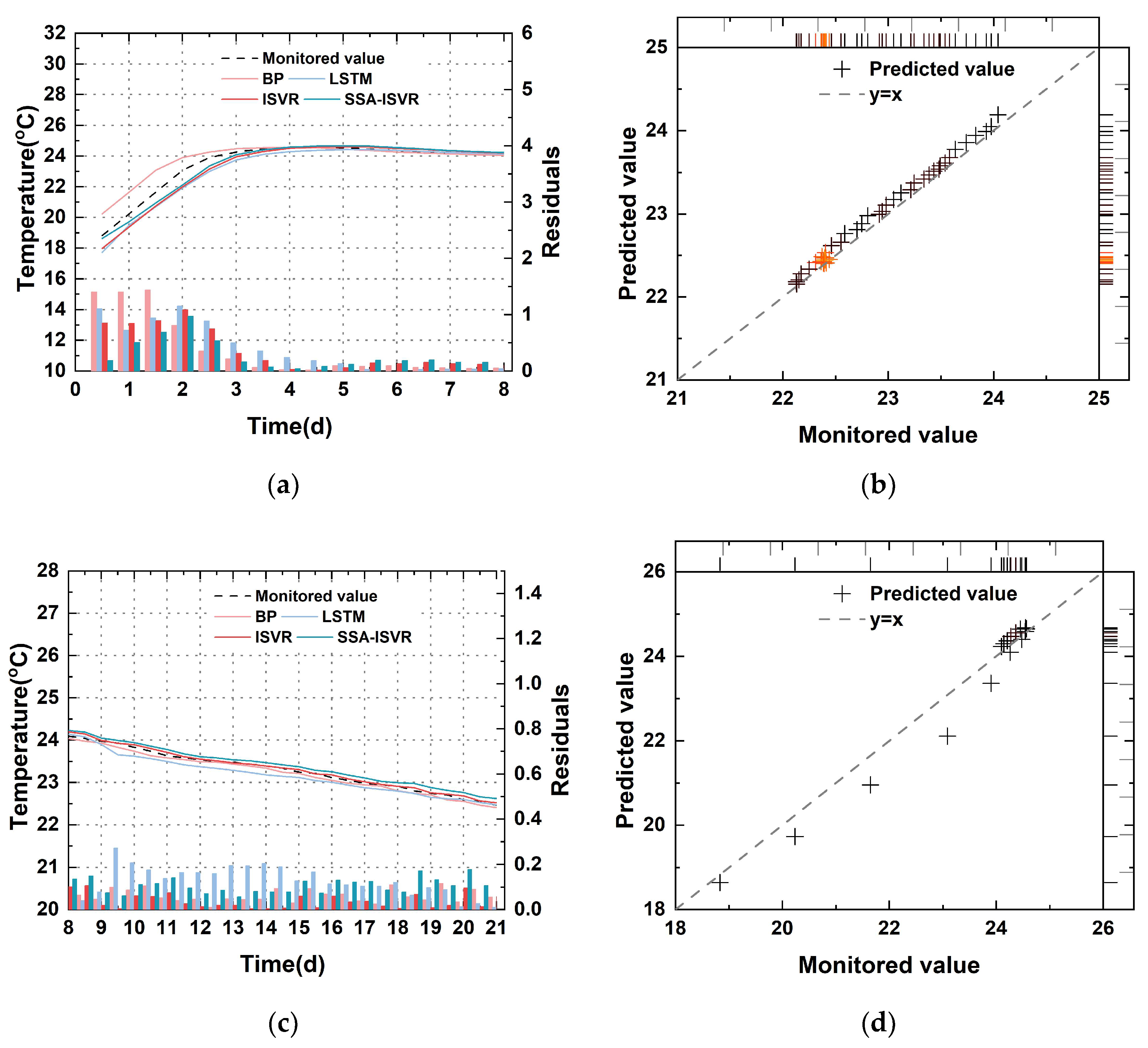
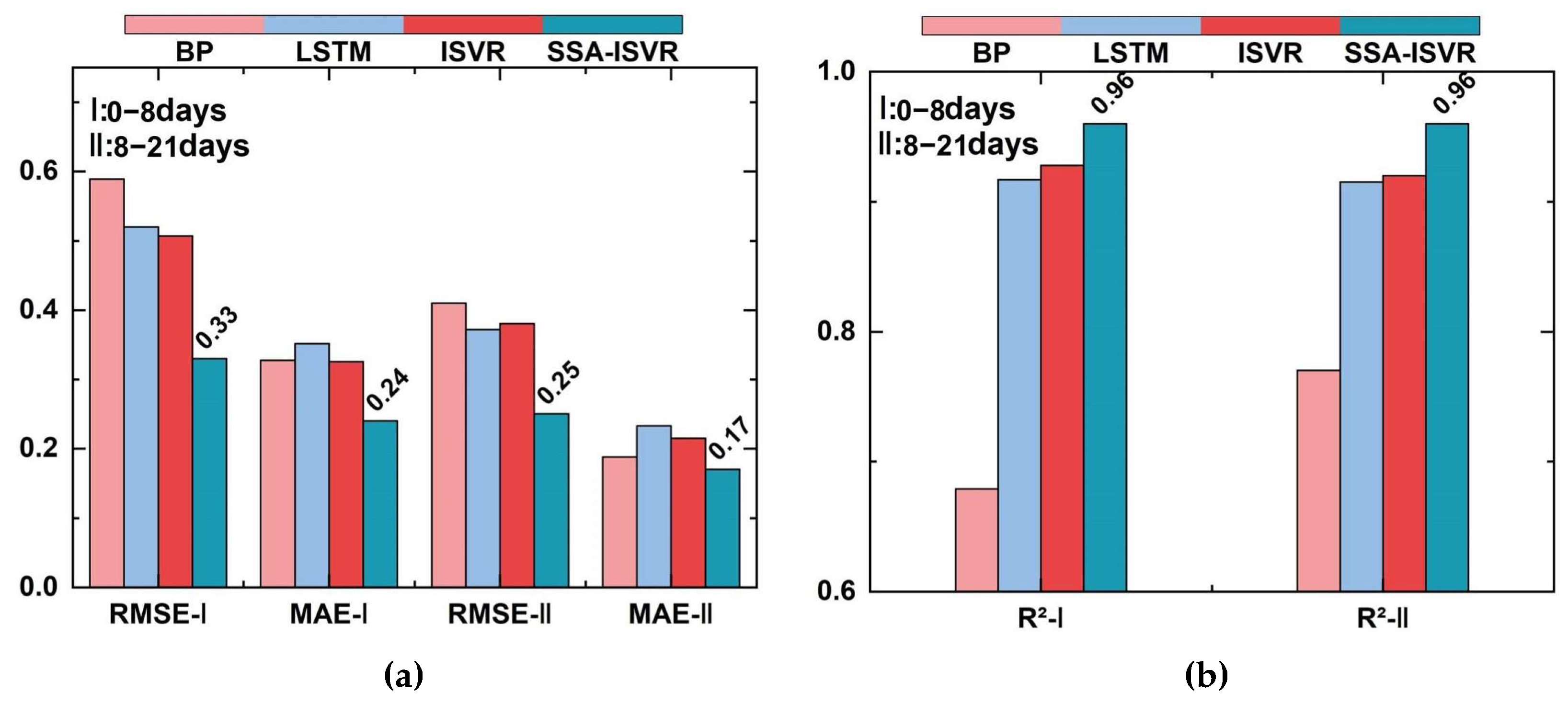
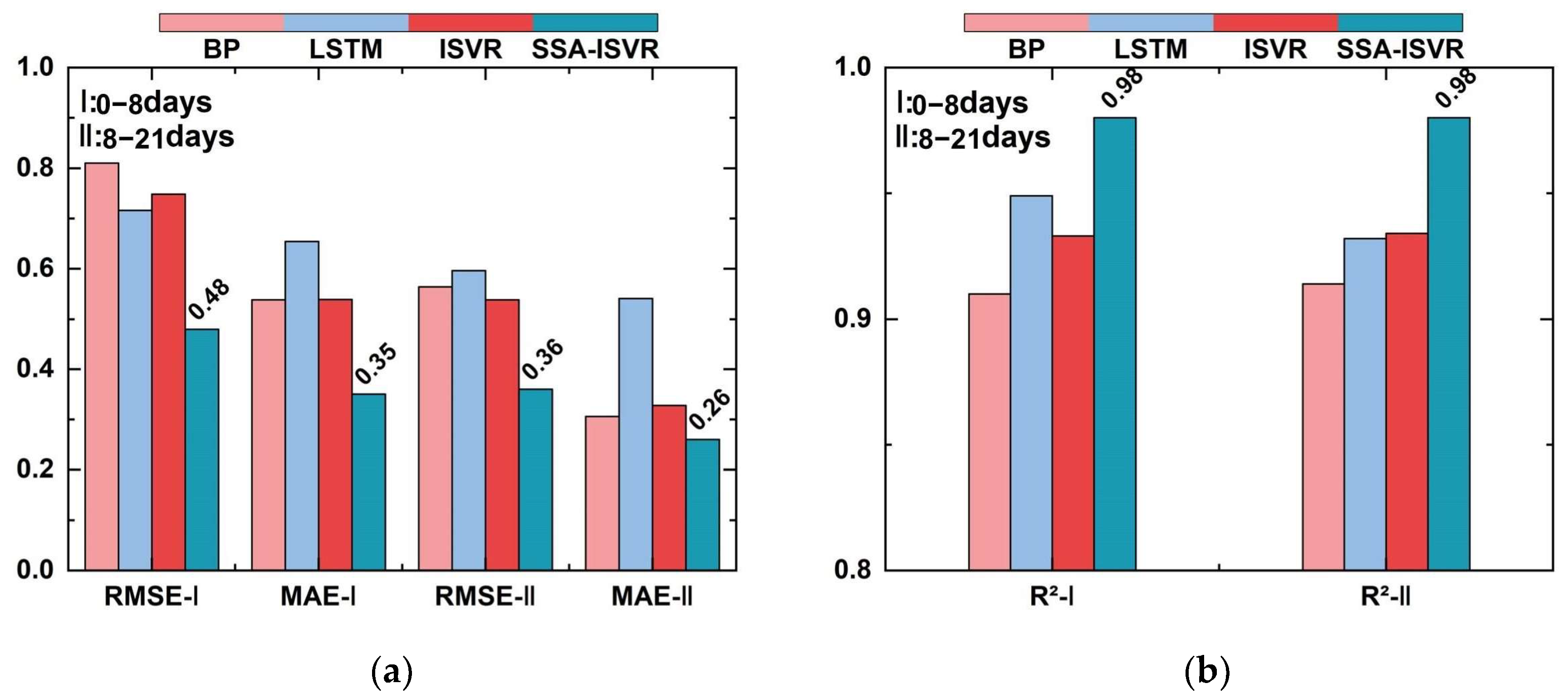
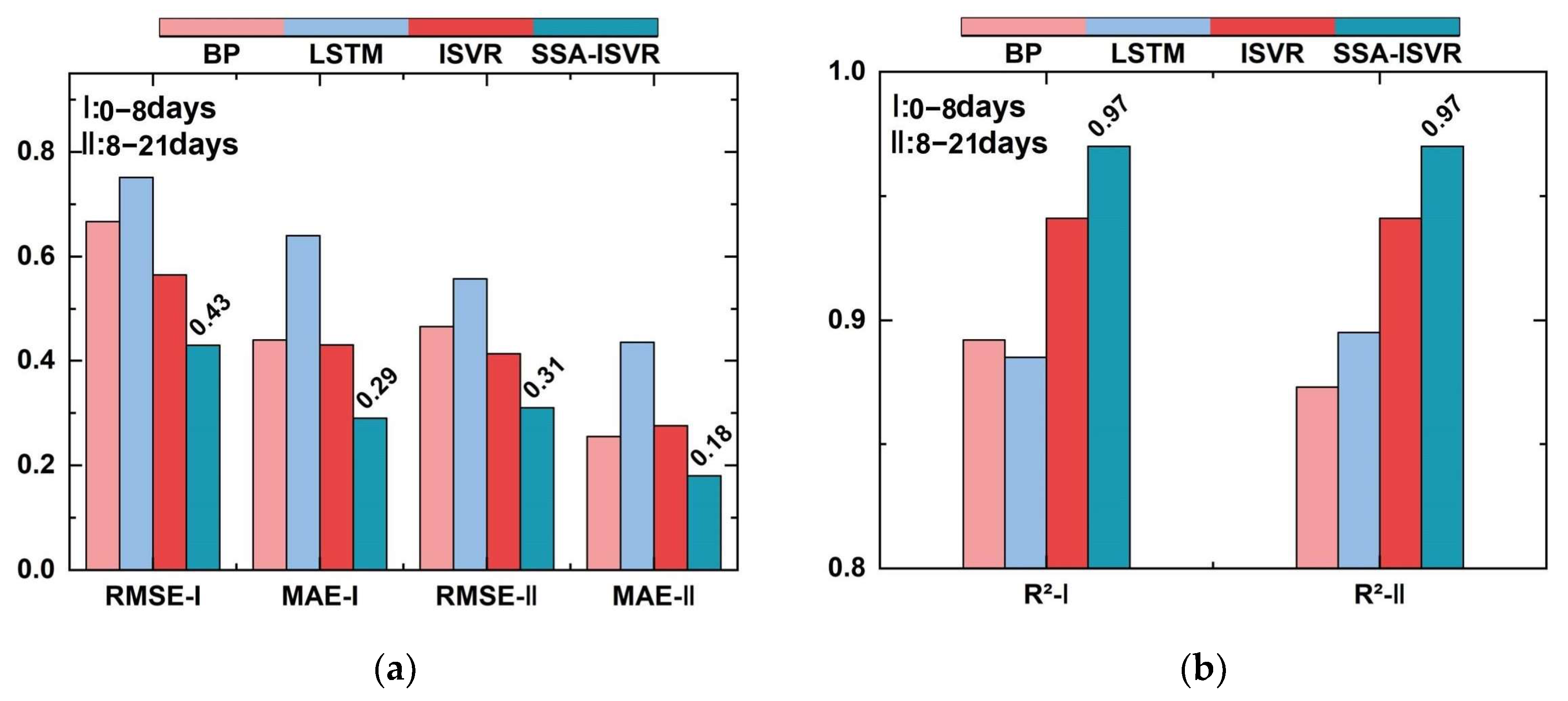
4.2.2. Comparison of Prediction Errors at Different Cooling Stages

Error analysis was conducted by dividing the 0–21-day period into two phases based on the intensity of the cement hydration reaction: the temperature rise period (0–8 days), characterized by an enhancement in hydration, and the temperature decline period (8–21 days), marked by a reduction in hydration activity. BP and LSTM are offline-trained models, whereas ISVR and SSA-ISVR are online-trained models.

Figure 13, Figure 14 and Figure 15 show the prediction results for typical pouring blocks across three dam segments.

Figure 13. Prediction results of models for the monitoring area in 7#-030: (a) temperature of the test set at 0–8 days; (b) the regression results of the SSA-ISVR model at 0–8 days; (c) temperature of the test set at 8–21 days; (d) the regression results of the SSA-ISVR model at 8–21 days.

Figure 14. Prediction results of models for the monitoring area in 11#-012: (a) temperature of the test set at 0–8 days; (b) the regression results of the SSA-ISVR model at 0–8 days; (c) temperature of the test set at 8–21 days; (d) the regression results of the SSA-ISVR model at 8–21 days.

Figure 15. Prediction results of models for the monitoring area in 17#-079: (a) temperature of the test set at 0–8 days; (b) the regression results of the SSA-ISVR model at 0–8 days; (c) temperature of the test set at 8–21 days; (d) the regression results of the SSA-ISVR model at 8–21 days.

The error evaluation metrics for training and predictions across different blocks using multiple models are detailed in Table 6, Table 7, Table 8 and Table 9 and illustrated in Figure 16, Figure 17 and Figure 18.

Table 6. Evaluation of different model training.

Train Sample Set	Algorithm	Training
		RMSE	MAE	R2
0–120 days	BP	0.137	0.070	0.995
	LSTM	0.231	0.139	0.985
	ISVR	0.161	0.109	0.990
	SSA-ISVR	0.189	0.080	0.994

Table 7. Evaluation of different model test samples in 7#-030.

Test Sample Set	Algorithm	Test
		RMSE	MAE	R2
0–8 days	BP	0.589	0.328	0.779
	LSTM	0.520	0.352	0.917
	ISVR	0.507	0.326	0.928
	SSA-ISVR	0.339	0.241	0.960
8–21 days	BP	0.410	0.188	0.870
	LSTM	0.372	0.233	0.915
	ISVR	0.381	0.215	0.920
	SSA-ISVR	0.248	0.173	0.958

Table 8. Evaluation of different model test samples in 11#-012.

Test Sample Set	Algorithm	Test
		RMSE	MAE	R2
0–8 days	BP	0.810	0.538	0.910
	LSTM	0.716	0.654	0.949
	ISVR	0.748	0.539	0.933
	SSA-ISVR	0.486	0.353	0.981
8–21 days	BP	0.564	0.306	0.914
	LSTM	0.596	0.541	0.932
	ISVR	0.538	0.328	0.934
	SSA-ISVR	0.361	0.263	0.980

Table 9. Evaluation of different model test samples in 17#-079.

Test Sample Set	Algorithm	Test
		RMSE	MAE	R2
0–8 days	BP	0.667	0.440	0.873
	LSTM	0.751	0.640	0.895
	ISVR	0.565	0.431	0.941
	SSA-ISVR	0.435	0.298	0.965
8–21 days	BP	0.466	0.255	0.892
	LSTM	0.557	0.436	0.885
	ISVR	0.414	0.276	0.941
	SSA-ISVR	0.307	0.179	0.966

Figure 16. Model evaluation in 7#-030: (a) RMSE and MAE of different models in two tests and (b) R² of different models in two tests.

Figure 17. Model evaluation in 11#-012: (a) RMSE and MAE of different models in two tests and (b) R² of different models in two tests.

Figure 18. Model evaluation in 17#-079: (a) RMSE and MAE of different models in two tests and (b) R² of different models in two tests.

According to results in Table 6, Table 7, Table 8 and Table 9, the pretrained model in this study achieved an $RMSE$ of 0.19 and an $MAE$ of 0.08 °C, making it slightly less effective than the BP model. The higher performance index on the training set comes from the fact that the training samples adequately reflect the overall distribution of the data. There is a significant statistical relationship between the variables, indicating that the model used has good fitting ability.

However, there are differences in the generalization performance of different models. In the 0–8-day and 8–21-day stages, the SSA-ISVR model achieved an average $RMSE$ of 0.20 and an average $MAE$ of 0.14 °C for temperature predictions across multiple blocks, yielding the best prediction accuracy across all tested sections. As demonstrated in Figure 13, Figure 14 and Figure 15, the online models generally exhibited smaller prediction errors. Figure 16, Figure 17 and Figure 18 illustrate the prediction results for blocks 17-079, 11-012, and 7-030, respectively, where I denotes the 0–8-day stage and II denotes the 8–21-day stage. Comparatively, the model developed in this study reduced the average $MAE$ by 31%, 44%, and 31% and the average $RMSE$ by 39%, 36%, and 30% in the 0–8-day stage, compared to the BP, LSTM, and ISVR models, respectively. During the 8–21-day stage, the average $MAE$ was reduced by 17%, 45%, and 25% and the average $RMSE$ by 37%, 39%, and 31%, compared to the BP, LSTM, and ISVR models, respectively. Furthermore, a paired t-test (p = 0.05) was conducted on the error indicators, and the results were all less than 0.05, suggesting that the differences between models are statistically significant.

During the 0–8-day period, it was difficult to accurately predict the true internal temperature of the concrete because of the intense cement hydration, resulting in generally large prediction errors across all models. During the 8–21-day period, as the hydration weakened, its influence on concrete temperature decreased, reducing the complexity of model features from a machine-learning perspective. This made it easier for the models to learn the process, thereby improving prediction accuracy and modeling efficiency.

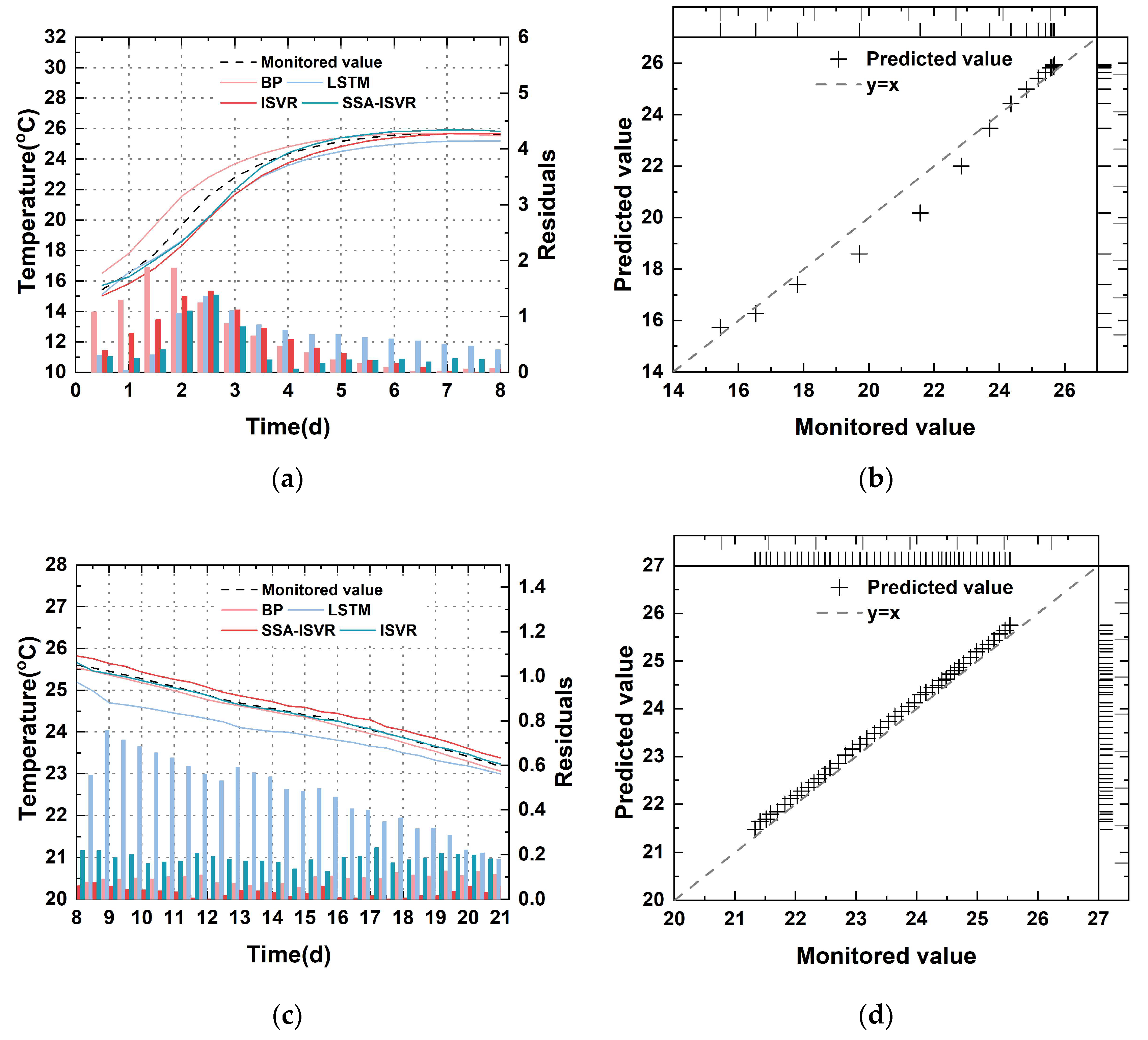
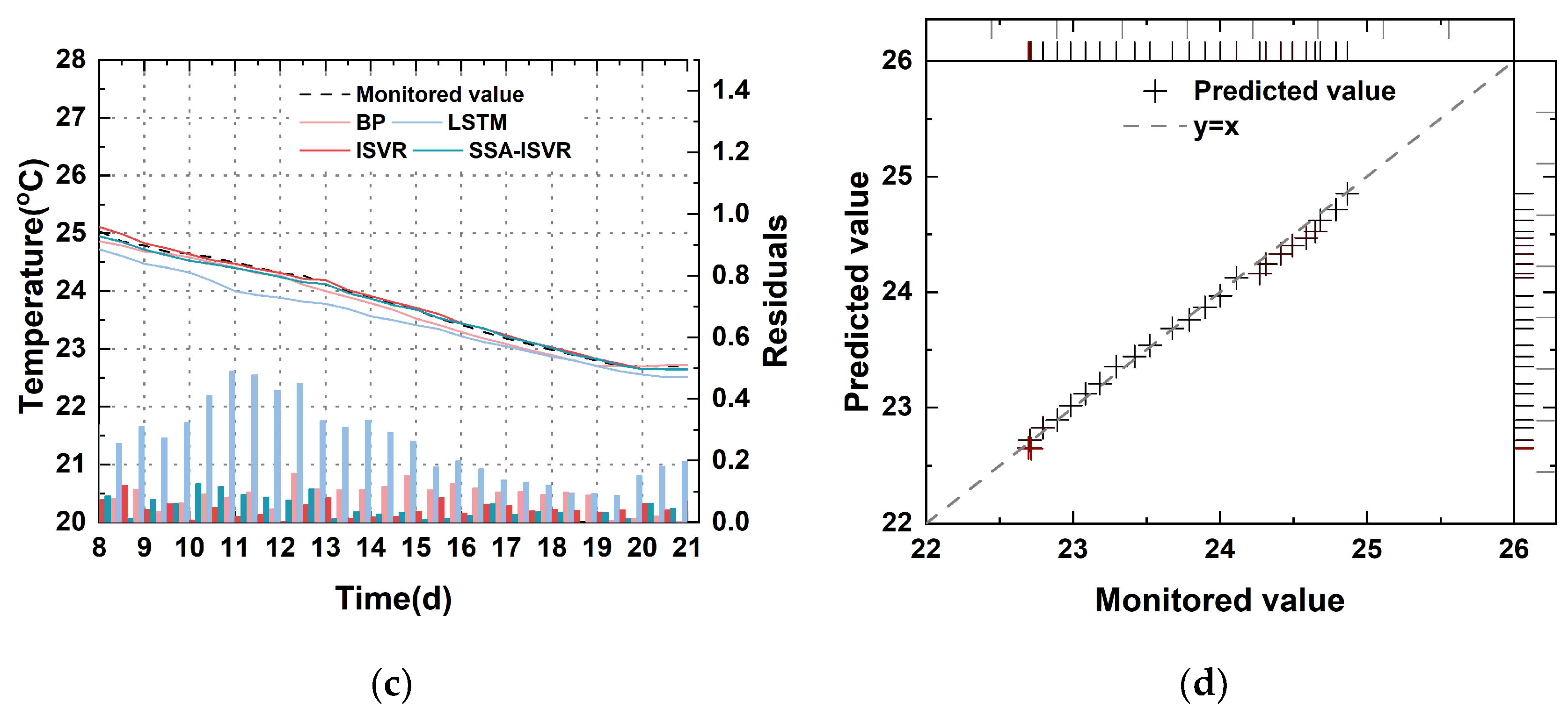
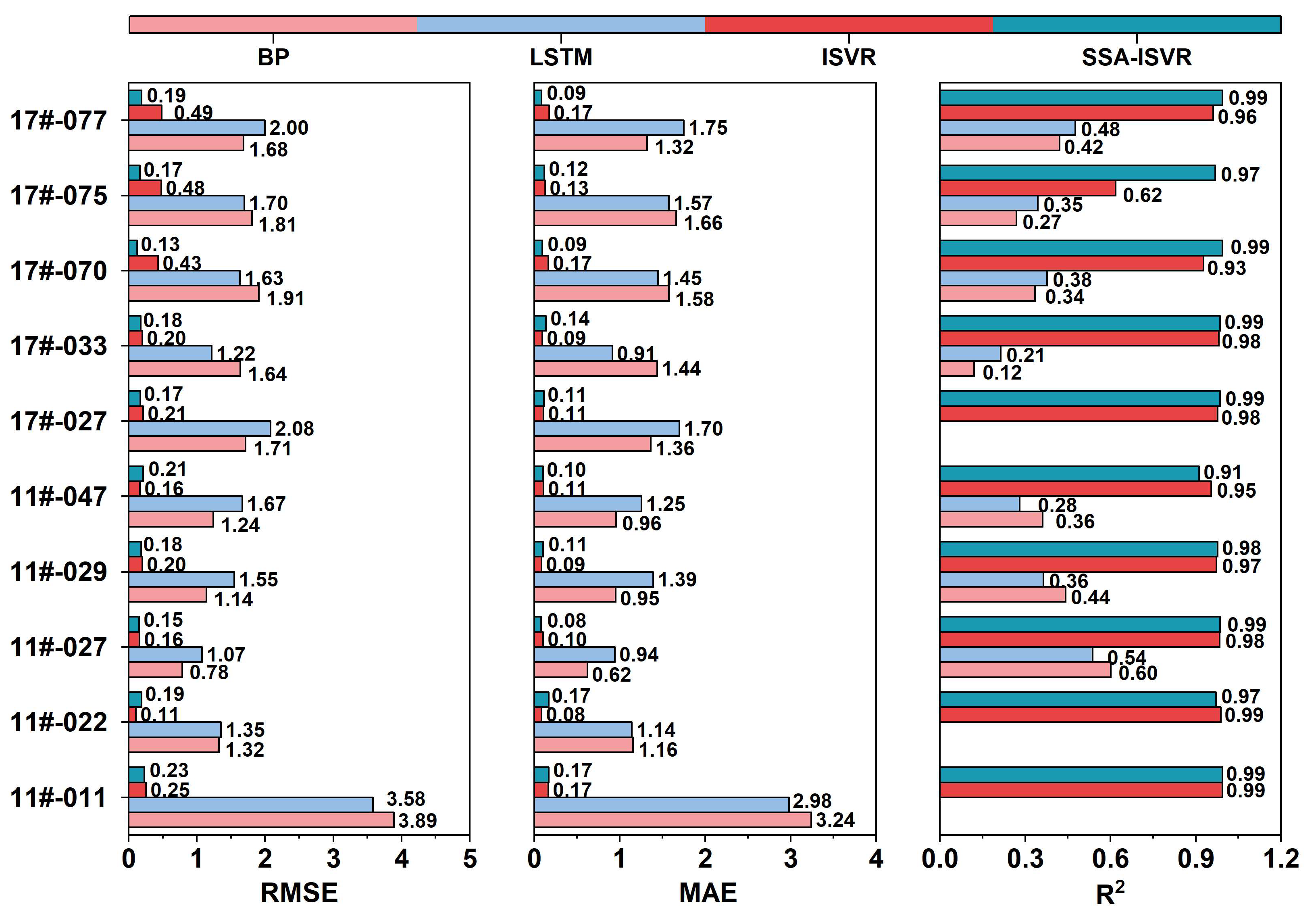
4.2.3. Evaluation of Model Generalization Using an Application Dataset

Section 4.2.1 and Section 4.2.2 demonstrate the accuracy and efficacy of our methodology, though the test set represents only a subset of scenarios. The trained framework was deployed to predict 120-day temperatures for 10 additional pouring blocks under varying operational conditions, including diverse materials, pouring timelines, and temperature control strategies, to further evaluate the proposed model’s generalization capability. Comparative analyses with the established models were conducted to compare their performances.

Quantitative comparisons of prediction accuracy between the proposed model and the other models (BP, LSTM, ISV, and SSA-ISVR) using this extended dataset are detailed in Figure 19.

Figure 19. Model evaluation in the extended application set.

The results indicate that the BP model achieved average $RMSE$ and $MAE$ values of 1.71 and 1.42 °C, respectively, with negative $R^2$ values for the three blocks. Negative $R^2$ values typically indicate severe underfitting or poor compatibility with the data characteristics; thus, negative values were set to zero in this study. The LSTM model demonstrated similar limitations, yielding an average $RMSE$ of 1.78, an average $MAE$ of 1.42 °C, and negative $R^2$ values for the same blocks. By contrast, the ISVR model significantly improved prediction accuracy, achieving an average $RMSE$ and $MAE$ of 0.27 and 0.13 °C, respectively, and an average $R^2$ of 0.93. The proposed SSA-ISVR model further enhanced prediction performance, achieving an average $RMSE$ of 0.17, an average $MAE$ of 0.10 °C, and an average $R^2$ of 0.97. These results demonstrate that offline models with fixed parameters possess limited predictive capability for concrete blocks, whereas the SSA-ISVR online model significantly improves prediction accuracy and better captures complex data characteristics.

4.3. Discussion

In arch dam construction, thermal stress due to improper temperature control is a significant cause of concrete cracking. Although recent advancements in dam temperature control technology based on real-time monitoring have effectively mitigated harmful thermal stress, such techniques lack predictive capability. This deficiency limits the accurate provision of control parameters, thereby increasing the potential risk of cracking. To address this issue, this study developed a rapid and precise online temperature prediction model (SSA-ISVR). The model was validated through practical engineering applications.

Section 4.2.1 and Section 4.2.2 present detailed comparisons between offline and online models under various operating conditions. The results indicate that the proposed SSA-ISVR online model achieves superior prediction accuracy and generalization capability. It successfully captures time-varying system characteristics and employs sample selection mechanisms (Section 2.3) to regulate sample capacity during online learning. Consequently, the model maintains strong generalization and reduces redundant features or efficiency loss. Through data-driven methods, the model provides precise predictions of future system states, thereby optimizing decision-making, enhancing efficiency, and reducing risks. Thus, it shows broad potential applications in engineering control, transportation scheduling, and other dynamic system identification fields.

This study has several limitations that warrant discussion:

(1)

The SSA optimization method was exclusively applied to the ISVR model. Although the ISVR model without SSA optimization demonstrated satisfactory performance in experiments, the efficacy of SSA optimization for other models remains to be validated.

(2)

While SSA parameter settings are relatively straightforward and can be informed by prior research, the methodology for selecting optimal parameters has not been thoroughly explored.

(3)

The impact of sample size on model performance requires additional examination. Substantial sample sizes may introduce redundancy and reduce modeling efficiency, whereas insufficient sample sizes could affect the model’s generalization capability.

Future research should focus on extending the SSA optimization framework to multiple machine learning models and verifying its generality through quantitative comparisons. It should also focus on adaptive optimization of optimizer parameters and sample sizes to reduce dependency. Adaptive control strategies and reinforcement learning mechanisms can be introduced to reduce the dependence on SSA initial parameter settings and SSA sample selection.

5. Conclusions

During arch dam construction, concrete temperature is subject to complex time-varying factors, making it challenging to achieve fast and accurate predictions. This study validated the rapid and precise predictive performance of the SSA-ISVR-based online prediction model for temperature forecasting during arch dam construction. Using the measured temperature data, the key parameters of the ISVR model are optimized with SSA, and the model is updated online according to the prediction error feedback to take the effect of time-varying factors into account with the online update of the model. The experimental results indicated the following:

• The proposed model achieved an average $RMSE$ of 0.20 and an $MAE$ of 0.14 °C between predicted and measured values across multiple blocks. This result suggested that during the initial cooling phase of concrete in arch dam construction, the SSA-ISVR model provided more accurate predictions than the BP, LSTM, and ISVR models.
• Across the two cooling phases of concrete within multiple blocks, the SSA-ISVR model reduced the average $MAE$ by 28% and the average $RMSE$ by 30%. This result demonstrated that the online temperature prediction model developed for arch dam construction exhibited greater generalizability than the offline models of BP and LSTM. The offline models struggled to adapt to new data patterns because of the cumulative effects of time-varying factors, which failed to decrease average prediction errors over time. In contrast, the online model was able to learn from model updates, thereby reducing prediction errors.
• Although numerical experiments demonstrated that the proposed model is a promising and effective approach for temperature prediction during concrete arch dam construction, some limitations may arise in practical applications. Given the complex construction conditions of concrete, additional features may be required to develop a temperature prediction model with higher adaptability. Future research could explore incorporating additional features to enhance the model’s learning capacity.

References

- Lin, P.; Ning, Z.; Shi, J.; Liu, C.; Chen, W.; Tan, Y. Study On the Gallery Structure Cracking Mechanisms and Cracking Control in Dam Construction Site. Eng. Fail. Anal. 2021, 121, 105135. [Google Scholar] [CrossRef]
- Li, M.; Lin, P.; Chen, D.; Li, Z.; Liu, K.; Tan, Y. An Ann-Based Short-Term Temperature Forecast Model for Mass Concrete Cooling Control. Tsinghua Sci. Technol. 2023, 28, 511–524. [Google Scholar] [CrossRef]
- Liu, J.; Wang, F.; Wang, X.; Hu, Z.; Liang, C. Temperature Monitoring and Cracking Risk Analysis of Corridor Top Arch of Baihetan Arch Dam During Construction Period. Eng. Fail. Anal. 2025, 167, 108903. [Google Scholar] [CrossRef]
- Nandhini, K.; Karthikeyan, J. The Early-Age Prediction of Concrete Strength Using Maturity Models: A Review. J. Build. Pathol. Rehabilit. 2021, 6, 7. [Google Scholar] [CrossRef]
- Zhu, Z.; Liu, Y.; Fan, Z.; Qiang, S.; Xie, Z.; Chen, W.; Wu, C. Improved Buried Pipe Element Method for Temperature-Field Calculation of Mass Concrete with Cooling Pipes. Eng. Comput. 2020, 37, 2619–2640. [Google Scholar] [CrossRef]
- Gao, X.; Li, Q.; Liu, Z.; Zheng, J.; Wei, K.; Tan, Y.; Yang, N.; Liu, C.; Lu, Y.; Hu, Y. Modelling the Strength and Fracture Parameters of Dam Gallery Concrete Considering Ambient Temperature and Humidity. Buildings 2022, 12, 168. [Google Scholar] [CrossRef]
- Chen, H.; Liu, Z. Temperature Control and Thermal-Induced Stress Field Analysis of Gongguoqiao Rcc Dam. J. Therm. Anal. Calorim. 2019, 135, 2019–2029. [Google Scholar] [CrossRef]
- Zhang, M.; Yao, X.; Guan, J.; Li, L. Study On Temperature Field Massive Concrete in Early Age Based On Temperature Influence Factor. Adv. Civ. Eng. 2020, 2020, 8878974. [Google Scholar] [CrossRef]
- Wang, F.; Zhang, A.; Fan, Y.; Zhou, Y.; Chen, J.; Tan, T. Temperature Monitoring Experiment and Numerical Simulation of the Orifice Structure in an Arch Dam Considering Solar Radiation Effects. J. Civ. Struct. Health Monit. 2023, 13, 523–545. [Google Scholar] [CrossRef]
- Žvanut, P.; Turk, G.; Kryžanowski, A. Thermal Analysis of a Concrete Dam Taking Into Account Insolation, Shading, Water Level and Spillover. Appl. Sci. 2021, 11, 705. [Google Scholar] [CrossRef]
- Hu, Y.; Bao, T.; Ge, P.; Tang, F.; Zhu, Z.; Gong, J. Intelligent Inversion Analysis of Thermal Parameters for Distributed Monitoring Data. J. Build. Eng. 2023, 68, 106200. [Google Scholar] [CrossRef]
- Bo, C.; Qingyi, W.; Weinan, C.; Hao, G. Optimized Inversion Method for Thermal Parameters of Concrete Dam Under the Insulated Condition. Eng. Appl. Artif. Intell. 2023, 126, 106898. [Google Scholar] [CrossRef]
- Wang, F.; Song, R.; Yu, H.; Zhang, A.; Wang, L.; Chen, X. Thermal Parameter Inversion of Low-Heat Cement Concrete for Baihetan Arch Dam. Eng. Appl. Artif. Intell. 2024, 131, 107823. [Google Scholar] [CrossRef]
- Mata, J. Interpretation of Concrete Dam Behaviour with Artificial Neural Network and Multiple Linear Regression Models. Eng. Struct. 2011, 33, 903–910. [Google Scholar] [CrossRef]
- Ranković, V.; Grujović, N.; Divac, D.; Milivojević, N. Development of Support Vector Regression Identification Model for Prediction of Dam Structural Behaviour. Struct. Saf. 2014, 48, 33–39. [Google Scholar] [CrossRef]
- Kang, F.; Liu, J.; Li, J.; Li, S. Concrete Dam Deformation Prediction Model for Health Monitoring Based On Extreme Learning Machine. Struct. Control Health Monit. 2017, 24, e1997. [Google Scholar] [CrossRef]
- Zhou, J.; Wang, Y.; He, X.; Huang, Y. Aasim, Rapid Prediction of the Highest Temperature of Concrete Block. Water Power 2013, 39, 46–48. [Google Scholar] [CrossRef]
- Zou, H.; Zhou, Y.; Wang, L.; Zhang, Z. Aasim, Prediction of the Maximum Temperature of the Concrete Pouring Bin of the Ultra-High Arch Dam Based On the Rbf-Bp Combined Neural Network Model. Water Resour. Power 2016, 34, 67–69. [Google Scholar] [CrossRef]
- Zhou, J.; Fan, S.; Fang, C.; Huang, Y.; Liu, F. Aasim, Prediction of the Maximum Temperature Inside the Concrete Pouring Bin Based On Random Forest Algorithm. Water Resour. Power 2024, 9, 84–87. [Google Scholar] [CrossRef]
- Wang, L.; Zhou, Y. Aasim, Application of Rbf Neural Network in the Prediction of the Maximum Temperature of the Concrete Pouring Chamber of the Extra-High Arch Dam. Water Resour. Power 2015, 33, 68–70. [Google Scholar] [CrossRef]
- Kang, F.; Li, J.; Dai, J. Prediction of Long-Term Temperature Effect in Structural Health Monitoring of Concrete Dams Using Support Vector Machines with Jaya Optimizer and Salp Swarm Algorithms. Adv. Eng. Softw. 2019, 131, 60–76. [Google Scholar] [CrossRef]
- Song, W.; Guan, T.; Ren, B.; Yu, J.; Wang, J.; Wu, B. Real-Time Construction Simulation Coupling a Concrete Temperature Field Interval Prediction Model with Optimized Hybrid-Kernel Rvm for Arch Dams. Energies 2020, 13, 4487. [Google Scholar] [CrossRef]
- Zhao, J.; Lv, Y.; Zeng, Q.; Wan, L. Online Policy Learning-Based Output-Feedback Optimal Control of Continuous-Time Systems. IEEE Trans. Circuits Syst. II Express Briefs 2024, 71, 652–656. [Google Scholar] [CrossRef]
- Fekri, M.N.; Patel, H.; Grolinger, K.; Sharma, V. Deep Learning for Load Forecasting with Smart Meter Data: Online Adaptive Recurrent Neural Network. Appl. Energ. 2021, 282, 116177. [Google Scholar] [CrossRef]
- Bayram, F.; Ahmed, B.S.; Kassler, A. From Concept Drift to Model Degradation: An Overview On Performance-Aware Drift Detectors. Knowl.-Based Syst. 2022, 245, 108632. [Google Scholar] [CrossRef]
- Malialis, K.; Panayiotou, C.G.; Polycarpou, M.M. Online Learning with Adaptive Rebalancing in Nonstationary Environments. IEEE Trans. Neural Netw. Learn. Syst. 2021, 32, 4445–4459. [Google Scholar] [CrossRef]
- Wassermann, S.; Cuvelier, T.; Mulinka, P.; Casas, P. Adaptive and Reinforcement Learning Approaches for Online Network Monitoring and Analysis. IEEE Trans. Netw. Serv. Manag. 2021, 18, 1832–1849. [Google Scholar] [CrossRef]
- Ma, J.; Theiler, J.; Perkins, S. Accurate On-Line Support Vector Regression. Neural. Comput. 2003, 15, 2683–2703. [Google Scholar] [CrossRef]
- Fan, J.; Xu, J.; Wen, X.; Sun, L.; Xiu, Y.; Zhang, Z.; Liu, T.; Zhang, D.; Wang, P.; Xing, D. The Future of Bone Regeneration: Artificial Intelligence in Biomaterials Discovery. Mater. Today Commun. 2024, 40, 109982. [Google Scholar] [CrossRef]
- Aniskin, N.; Trong, C.; Quoc, L. Influence of Size and Construction Schedule of Massive Concrete Structures On its Temperature Regime. MATEC Web Conf. 2018, 251, 02014. [Google Scholar] [CrossRef]
- Feng, W.; Wang, J.; Chen, H. A fast SVR incremental learning algorithm. J. Chin. Comput. Syst. 2015, 36, 162–166. [Google Scholar] [CrossRef]
- Li, G.; Jiang, Y.; Fan, L.; Xiao, X.; Wang, D.; Zhang, X. Constitutive Model of 25Crmo4 Steel Based On Ipso-Svr and its Application in Finite Element Simulation. Mater. Today Commun. 2023, 35, 106338. [Google Scholar]
- Xue, J.; Shen, B. A Novel Swarm Intelligence Optimization Approach: Sparrow Search Algorithm. Syst. Sci. Control Eng. 2020, 8, 22–34. [Google Scholar] [CrossRef]
- Fan, Y.; Zhang, Y.; Guo, B.; Luo, X.; Peng, Q.; Jin, Z. A Hybrid Sparrow Search Algorithm of the Hyperparameter Optimization in Deep Learning. Mathematics 2022, 10, 3019. [Google Scholar] [CrossRef]
- Laskov, P.; Gehl, C.; Krüger, S.; Müller, K.R.; Bennett, K.P.; Parrado-Hernández, E. Incremental Support Vector Learning: Analysis, Implementation and Applications. J. Mach. Learn. Res. 2006, 7, 1909–1936. [Google Scholar]
- Carmichael, I.; Marron, J.S. Geometric Insights Into Support Vector Machine Behavior Using the KKT Conditions. arXiv 2017, arXiv:1704.00767. [Google Scholar] [CrossRef]
- Zhou, W.; Zhang, L.; Jiao, L. Aasim, An Analysis of Svms Generalization Performance. Acta Electron. Sin. 2001, 29, 590–594. [Google Scholar] [CrossRef]
- Pan, T.; Li, S. Generalised Predictive Control for Non-Linear Process Systems Based On Lazy Learning. Int. J. Model. Identif. Control 2006, 1, 230–238. [Google Scholar] [CrossRef]
- Cheng, C.; Chiu, M. A New Data-Based Methodology for Nonlinear Process Modeling. Chem. Eng. Sci. 2004, 59, 2801–2810. [Google Scholar] [CrossRef]
- Liang, Z.; Zhao, C.; Zhou, H.; Liu, Q.; Zhou, Y. Error Correction of Temperature Measurement Data Obtained From an Embedded Bifilar Optical Fiber Network in Concrete Dams. Measurement 2019, 148, 106903. [Google Scholar] [CrossRef]
- Abbas, Z.H.; Majdi, H.S. Study of Heat of Hydration of Portland Cement Used in Iraq. Case Stud. Constr. Mat. 2017, 7, 154–162. [Google Scholar] [CrossRef]
- Zhang, Z.; Scherer, G.W.; Bauer, A. Morphology of Cementitious Material During Early Hydration. Cem. Concr. Res. 2018, 107, 85–100. [Google Scholar] [CrossRef]
- Scrivener, K.; Ouzia, A.; Juilland, P.; Kunhi Mohamed, A. Advances in Understanding Cement Hydration Mechanisms. Cem. Concr. Res. 2019, 124, 105823. [Google Scholar] [CrossRef]
- Qiang, S.; Xie, Z.; Zhong, R. A P-Version Embedded Model for Simulation of Concrete Temperature Fields with Cooling Pipes. Water Sci. Eng. 2015, 8, 248–256. [Google Scholar] [CrossRef]
- Pouya, M.R.; Sohrabi-Gilani, M.; Ghaemian, M. Thermal Analysis of Rcc Dams During Construction Considering Different Ambient Boundary Conditions at the Upstream and Downstream Faces. J. Civ. Struct. Health Monit. 2022, 12, 487–500. [Google Scholar] [CrossRef]
- Han, S.; Qubo, C.; Meng, H. Parameter Selection in SVM with RBF Kernel Function; World Automation Congress: Puerto Vallarta, Mexico, 2012. [Google Scholar]
- Achirul Nanda, M.; Boro Seminar, K.; Nandika, D.; Maddu, A. A Comparison Study of Kernel Functions in the Support Vector Machine and its Application for Termite Detection. Information 2018, 9, 5. [Google Scholar] [CrossRef]
- Liu, D.; Zhang, W.; Tang, Y.; Jian, Y. Prediction of Hydration Heat of Mass Concrete Based On the SVR Model. IEEE Access 2021, 9, 62935–62945. [Google Scholar] [CrossRef]
Disclaimer/Publisher’s Note: The statements, opinions and data contained in all publications are solely those of the individual author(s) and contributor(s) and not of MDPI and/or the editor(s). MDPI and/or the editor(s) disclaim responsibility for any injury to people or property resulting from any ideas, methods, instructions or products referred to in the content. |
© 2025 by the authors. Licensee MDPI, Basel, Switzerland. This article is an open access article distributed under the terms and conditions of the Creative Commons Attribution (CC BY) license (https://creativecommons.org/licenses/by/4.0/).