Demonstration of an Advanced Rectification Strategy on a Linear Generator for Better Electricity Quality

Abstract

This paper focuses on the challenges of the free-piston internal combustion linear power generation system, which is characterized by a wide frequency and amplitude variation range of output electric power and difficulties in rectification. The study delves into the power generation characteristics during the system’s stable operation and explores strategies for rectifying three-phase electric power. A mathematical model of the power generation system has been established. The model of the linear motor has been verified, and an in-depth analysis of the electric power output characteristics has been carried out. On this basis, this paper proposes several rectification schemes, including uncontrolled rectification, PWM rectification based on a PI control strategy, and compound control based on model predictive sliding mode control. In terms of control strategy, a model predictive sliding mode compound control algorithm is introduced to optimize traditional PWM rectification. By comparing and analyzing the electric power output effects under different rectification schemes, this paper aims to explore the rectification strategy most suitable for the system. Simulation results indicate that while uncontrolled rectification can achieve power conversion, it leads to further phase current distortion on the linear motor side. This paper examines the last two types of rectification strategies in terms of robustness, accuracy, and responsiveness. It is found that model predictive sliding mode compound control performs better than PI control. It can stably regulate the output voltage, and the phase current on the linear motor side will not be distorted. It is more suitable for power processing in this system.

1. Introduction

The free-piston linear power generation system (FPLG) [1,2,3] differs from conventional rotary reciprocating internal combustion engines by eliminating the crank-connecting rod mechanism. It uses controlled alternate firing of the opposed-free piston engine [4,5] to drive the pistons’ reciprocating motion, moving the linear motor’s mover to cut magnetic flux lines and generate electromotive force, as shown in Figure 1. The FPLG has a more compact structure with high power density. Its modular design suits distributed drive. It also has a flexibly adjustable compression ratio, multi-fuel adaptability [6,7], and can operate in various combustion modes. However, in actual operation, the lack of a crank-connecting rod structure complicates the piston motion, and this uncertainty becomes a technical bottleneck. It also makes the linear motor’s electrical output characteristics [8] differ from those of conventional rotary motors. The composition of the FPLG system and the overall structure of the rectification control strategy adopted in this paper are shown in Figure 1.

The research on Free-Piston Linear Generators (FPLG) primarily focuses on fuel adaptability, system operating characteristics, and stability control [9,10,11]. These studies are often based on piston motion, structural design, and material selection for the linear generator. However, there has been limited research on the power consumption systems at the backend and their impact on system performance and matching. Additionally, thermodynamic or combustion characteristics related to FPLG have been investigated to simplify the design of the backend load. Pure resistive loads are commonly used to dissipate electrical energy, and the output power [12,13,14,15] at the load terminal is considered as the system’s output power. To enhance system stability and reduce failures, researchers often choose to control the current to achieve precise piston trajectories or maintain the piston at the dead center within the generator [16]. This strategy typically aims at piston stability or precise trajectory control to manage the generator’s output characteristics.

As research on FPLG operating characteristics progresses, some scholars have found that the system can operate continuously with minimal intervention [17]. This finding accelerates the viability of FPLG in hybrid vehicles and highlights the need to consider the generator system’s output characteristics. The adaptability of FPLG to different operating conditions and energy consumption profiles must be carefully matched.

Uncontrolled rectification can convert the three-phase AC from the linear motor into pulsating DC. Its advantages are a simple structure and no need for complex control strategies. However, the quality of the output DC needs improvement. Three-phase controlled rectification, or Pulse Width Modulation Control (PWMC) [18,19,20], regulates the AC voltage and current by controlling the switching of three-phase bridge arms. It uses PI-based dual closed-loop control [21,22] for voltage and current. This method can stabilize and adjust the DC voltage but has a complex control structure. The system’s response speed and anti-interference ability are also weak.

To address these issues, this paper designs a model predictive control (MPC) controller [23,24] for the FPLG system. It reduces algorithm optimization steps and improves steady-state performance. An integral sliding mode control algorithm replaces the traditional PI control in the voltage outer loop, forming the Model Predictive Sliding Mode Control (MPSMC) [25,26,27,28,29]. This compound control simplifies controller parameter tuning, enhances anti-interference and adaptability, and makes the output voltage and frequency highly controllable, better matching the FPLG system’s working characteristics.

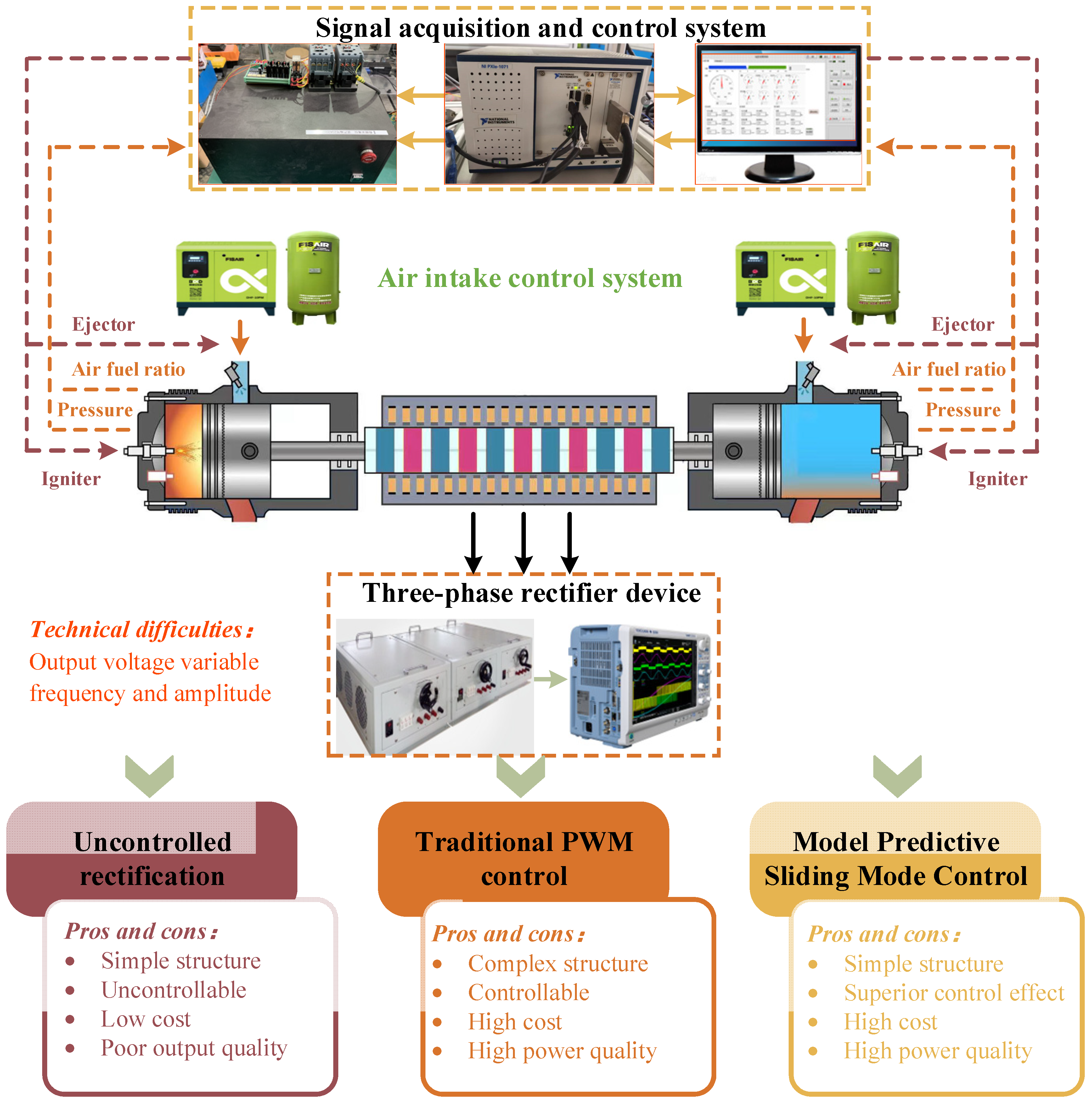
2. Analysis of the FPLG System Working Process

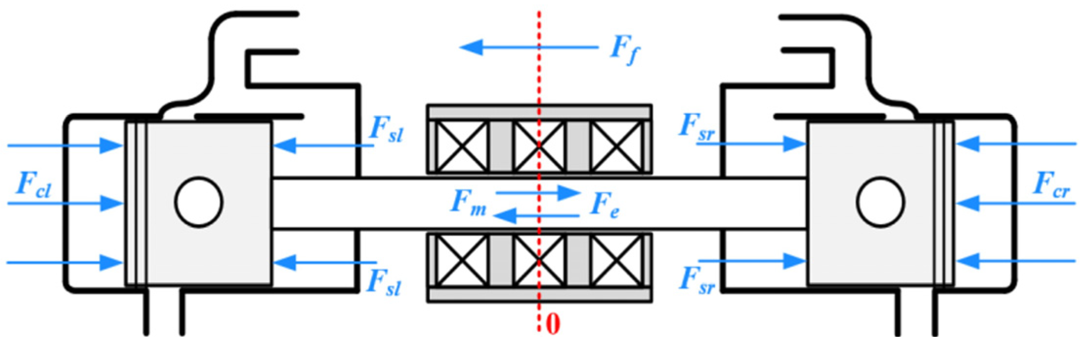
2.1. Working Principle of the Power Generation System

The free-piston linear internal combustion power generation system comprises an intake system, an FPLG prototype, a power conversion device, and a signal acquisition and control system, as shown in Figure 1. The FPLG prototype consists of two opposed free-piston engines and a linear motor, with the motor’s mover connected to the pistons via a connecting rod. The system operates in two modes: cold start and stable power generation. During the cold start phase, the linear motor functions as a driver, using its moving part to move the pistons. This compresses the fuel-air mixture in the cylinders. Once ignition conditions are met, the engine ignites and transitions to stable power generation. Here, the linear motor acts as a generator.

2.2. Linear Motor Modeling

In this paper, the chosen linear motor is a cylindrical three—phase permanent magnet synchronous one. To precisely describe its power generation output characteristics, it’s essential to conduct mathematical modeling and analysis. The voltage equation of the linear motor in the three—phase stationary ABC coordinate system is as follows:

$$\left\{\begin{array}{c}{u}_a=R_s·i_a+L_s·{\displaystyle \frac{{di}_{sa}}{dt}}+e_a\\ u_b=R_s·i_b+L_s·{\displaystyle \frac{{di}_{sb}}{dt}}+e_b\\ u_c=R_s·i_c+L_s·{\displaystyle \frac{{di}_{sc}}{dt}}+e_c\end{array}\right.$$

(1)

In the formula, $u_a$, $u_b$, and $u_c$ are the phase voltages of the linear motor, $R_s$ is the phase resistance of each phase winding, $L_s$ is the phase inductance of each phase winding, and $e_a$, $e_b$, and $e_c$ are the back electromotive forces. Their magnitude is directly correlated with the position of rotor, motion speed, and magnetic flux. Its mathematical expression is:

$$\left\{\begin{array}{l}{e}_a=-{\psi }_f\times {\displaystyle \frac{\pi \times v}{\tau }}\times \mathit{sin}(\theta +{\theta }_0)\\ e_b=-{\psi }_f\times {\displaystyle \frac{\pi \times v}{\tau }}\times \mathit{sin}(\theta +{\theta }_0-{\displaystyle \frac{2}{3}}\pi )\\ e_c=-{\psi }_f\times {\displaystyle \frac{\pi \times v}{\tau }}\times \mathit{sin}(\theta +{\theta }_0+{\displaystyle \frac{2}{3}}\pi )\end{array}\right.$$

(2)

In the formula, ${\psi }_f$ is the peak magnetic flux of the permanent magnet, $v$ is the velocity of the rotor motion $\theta$ From an electrical perspective ${\theta }_0$ is the initial electrical angle.

The core difference between linear and rotary motors lies in the mover’s motion type. To compare them equivalently, ensure that within the same operating cycle, the linear motor’s mover and the rotary motor’s rotor travel the same displacement length. The conversion relationship is as follows:

$$\left\{\begin{array}{l}{\displaystyle \frac{\theta \times r}{2p\pi \times r}}={\displaystyle \frac{x}{2p\tau }}\\ x={\displaystyle \frac{\theta \times \tau }{\pi }}\end{array}\right.$$

(3)

In the formula, $p$ is the number of pole pairs of the linear motor $\tau$ for polar distance $\omega$ To induce the angle of electromotive force. The rotating motor scans $p$ pairs of permanent magnets every time it rotates, which is equivalent to the displacement of $p$ pairs of permanent magnet pole distances by the linear motor moving in one direction. Similarly, the conversion relationship between the speed of the linear motor rotor and the equivalent rotational speed is:

$$v={\displaystyle \frac{\omega \times \tau }{\pi }}$$

(4)

Therefore, the general expression for the thrust of a linear motor is:

$$F_e={\displaystyle \frac{3}{2}}\times {\displaystyle \frac{\pi }{\tau }}\times {\displaystyle \frac{\pi }{r}}\times \left({\phi }_d{i}_q-{\phi }_q{i}_d\right)$$

(5)

Linear motors generally adopt a control strategy with rotor flux orientation $i_d=0$, so that the electromagnetic thrust of the motor is only proportional to the amplitude of the stator current:

$$F_e={\displaystyle \frac{3}{2}}\times {\displaystyle \frac{\pi }{\tau }}\times {\displaystyle \frac{\pi }{r}}\times {\phi }_d{i}_q=K_f{i}_q$$

(6)

In the formula, $k_f$ is the electromagnetic thrust coefficient of the motor.

The coupled dynamic model involved in the entire working process of the system exhibits nonlinear characteristics. During the motion of the piston mover assembly, various forms of energy flow through this assembly within the system, facilitating the transfer and conversion of energy. These energies collectively drive the piston mover assembly to perform cyclic motion. The structure and motion form of the linear motor are shown in Figure 2.

Since the structure is not constrained by a crank-connecting rod mechanism, its motion is governed solely by the resultant force acting on the piston and mover. The piston mover assembly is subjected to the forces from the gas pressure in the two cylinders, frictional forces, and the thrust of the linear motor. The dynamic equation of the piston mover assembly is as follows:

$$m{\displaystyle \frac{d^{2}x}{d^{2}t}}=F_{cl}+F_{cr}+F_f+F_e$$

(7)

In the formula, $F_{cl}$ is the gas pressure of the right cylinder, $F_{cr}$ is the gas pressure of the right cylinder, $F_f$ is the frictional force generated by the movement of mechanical components, $F_e$ is the electromagnetic resistance in linear motors.

In the preceding text, the construction of subsystem models within the system was detailed. Now, parameter matching for these models is conducted. The key structural parameters of the system are presented in

Table 1. System Parameter Matching Design.

Design Parameters	Parameter	Design Parameters	Parameter
Mass of moving sub component/kg	3.75	Maximum travel distance/mm	80
Cylinder diameter/m	0.051	Cylinder depth/m	0.029
Line resistance/Ohm	10.16	Line inductance/mH	12.78
Motor thrust constant/N/A	78.9	Permanent magnet magnetic flux	0.24

.

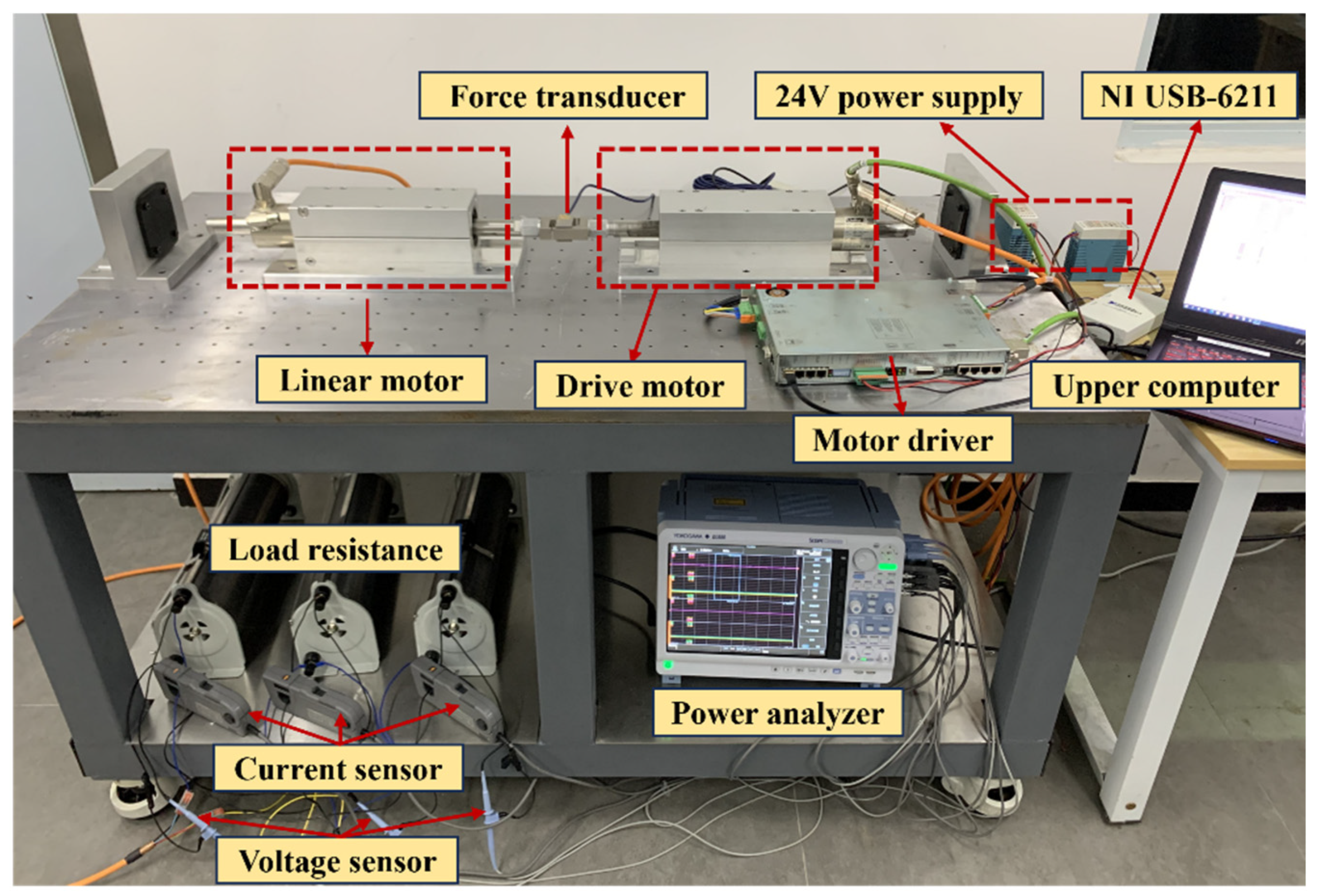
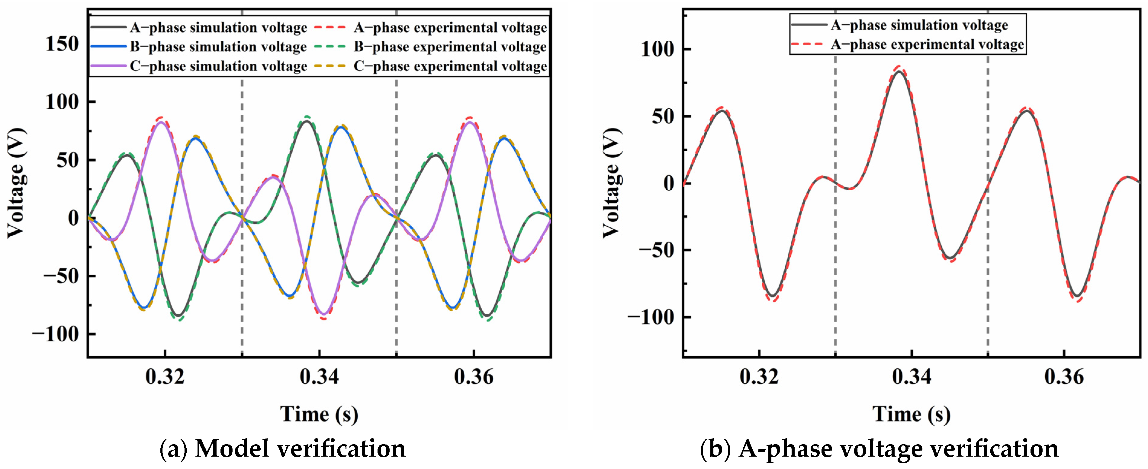
2.3. Linear Motor Model Verification

Model validation of the linear motor is conducted on an existing linear motor test bench, illustrated in Figure 3. The setup includes two linear motors (one as a motor and the other as a generator), a motor driver, a power supply, host computer software, three sliding rheostats, and a power analyzer. During the experiment, the host computer software generates displacement profiles with specified frequency and stroke. The motor driver ensures the motor drives the generator’s mover to follow the reference profile. Once stable operation is achieved, an external three-phase resistor is connected. The power analyzer measures the terminal voltage across the resistor, the three-phase current in the circuit, and the output power at the load. The collected data is then imported into data processing software for analysis. The parameters of each component on the test bench are listed in

Table 2. Experimental Bench Instrument Models.

Equipment	Type	Parameter
Drive motor	P10 series	Peak force: 1600 N; Peak speed: 6.5 m/s; Peak current: 20 A; $\pm$20 μm
Motor driver	E1400 series	32 bit; 3 $\times$ 400/480 VAC; Supply voltage: 24 V
Power analyzer	Yokogawa DL950	200 MS/s Sampling rate; 14 bit; 10 GE Data transmission rate; 8 G Point memory
Current sensor	Yokogawa probes	$\pm$150 Arms; 10 MHz; 1% Accuracy
Voltage sensor	Yokogawa probes	±1000 Vpeak; 60 MHz; 10: 1
Electromagnetic force sensor	HBM S9N	1 kN; 0.02%FS; 2 MV/V
Data acquisition instrument	NI USB-6211	250 kS/s; 16 bit

.

This test examines the power generation characteristics under an external linear load. The motor mover’s displacement reference profile is a standard sine wave, with a stroke of 50 mm and a frequency of 10 Hz. The external load is 50 Ω. Figure 4 a compares the experimental and simulated load—end voltages under these conditions. It shows the voltage in phases A, B, and C (Figure 4). Within one motor operation cycle, the simulated and experimental load—end voltages closely match in peak value and phase. The peak voltage error is 2.1 V, an error rate of about 2.56%.

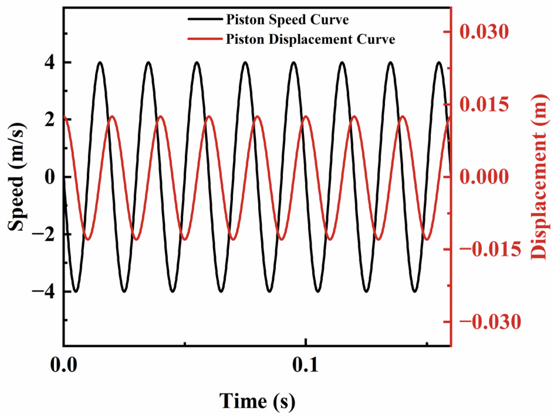
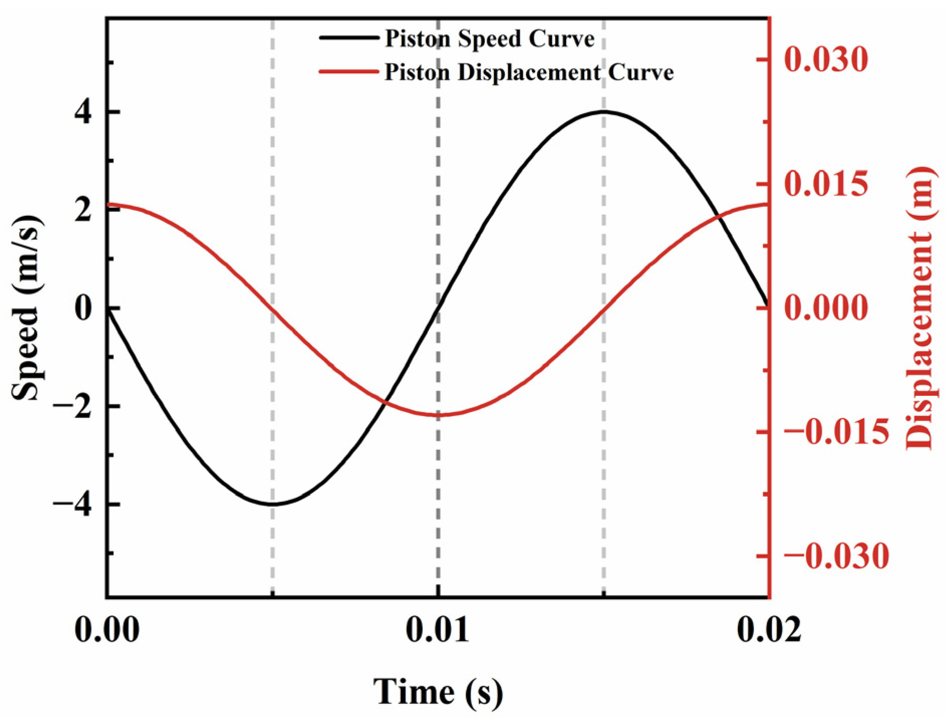
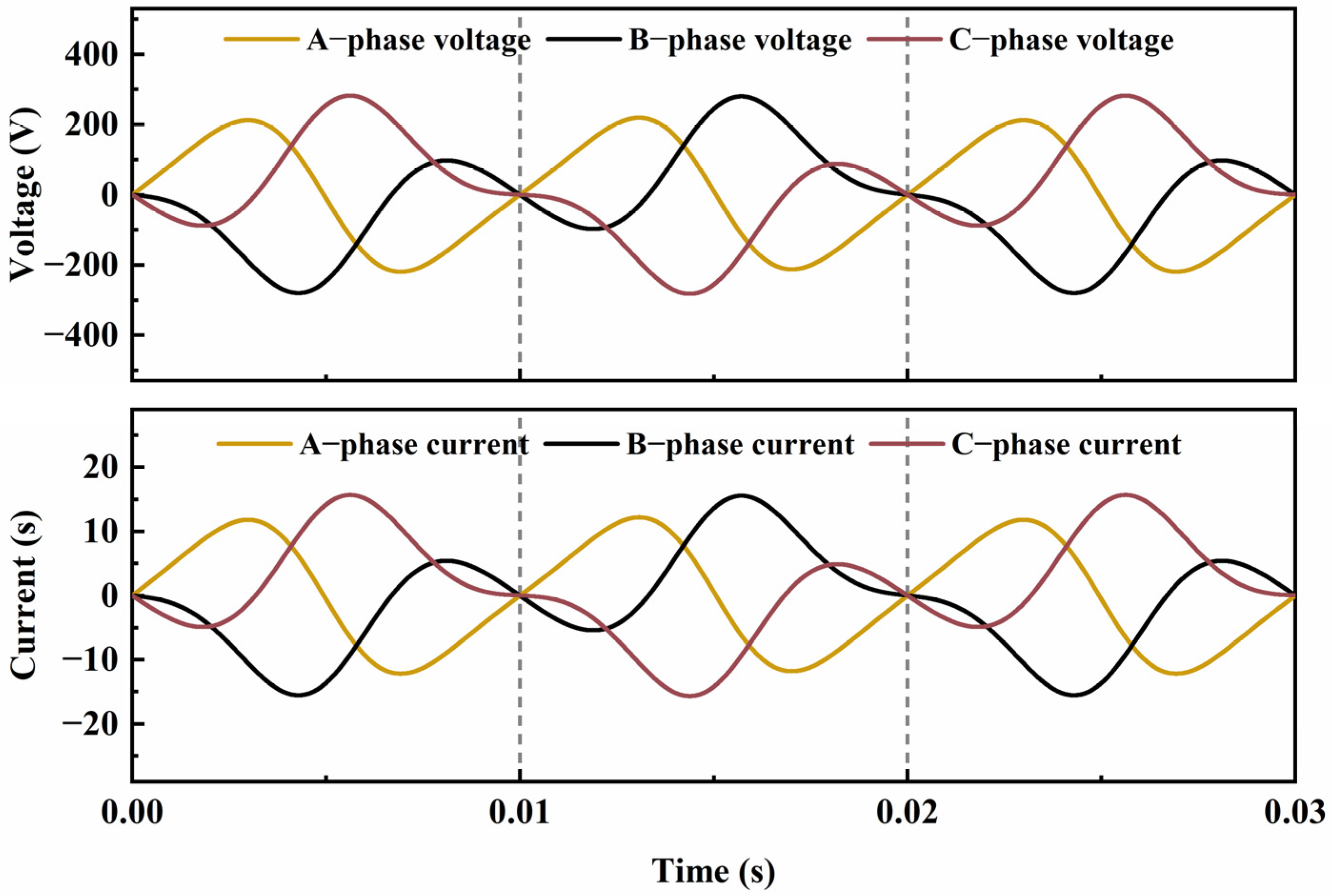
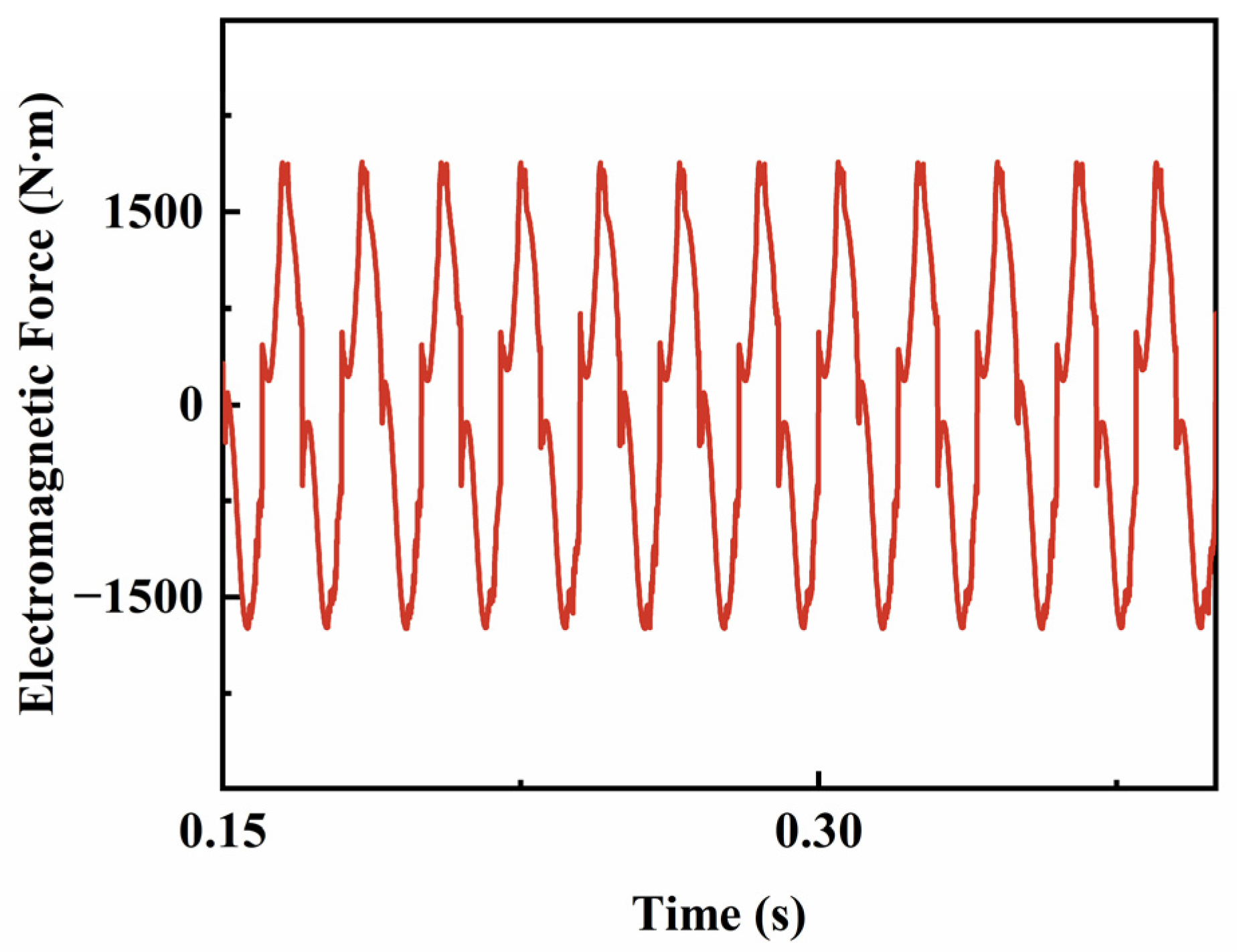
2.4. Analysis of Linear Motor Output Characteristics

Based on the modeling and analysis of the linear motor, a mathematical model of the permanent magnet synchronous linear motor was developed in Matlab/Simulink (2022b). This model uses the position and velocity of the motor mover as inputs. Combining data on the mover’s velocity, position, and the peak value of flux linkage, it calculates the three-phase induced electromotive force in the motor. After passing through the motor’s coils, this induced electromotive force is output as corresponding phase voltages and currents.

The system’s input signals are shown in Figure 5. The mover has a stroke of 25 mm and operates at a frequency of 50 Hz. Its velocity and displacement changes over a single cycle are depicted in Figure 6. The three-phase voltage and current curves output by the linear motor under these conditions are shown in Figure 7. While the voltage shows periodic changes, it differs from the traditional sine curve. When the motor reaches the top and bottom dead centers and changes direction, the phase sequence of the generated voltage alters, and all three phases converge at zero. This is because at the phase—changing points, the mover doesn’t cut the magnetic flux, resulting in zero induced electromotive force in the circuit. When the motor isn’t at the dead centers and the mover moves in one direction, its motion resembles that of a rotary motor, producing a waveform similar to a sine curve. The electrical angles of each phase differ by 120°, except when the linear motor’s velocity is zero. At any moment, the phase voltages are symmetrical. The electromagnetic thrust of the motor under these conditions is shown in Figure 8, with a peak value of 2000 N·m.

3. Optimization of Controllable Rectification Based on Advanced Control Strategies

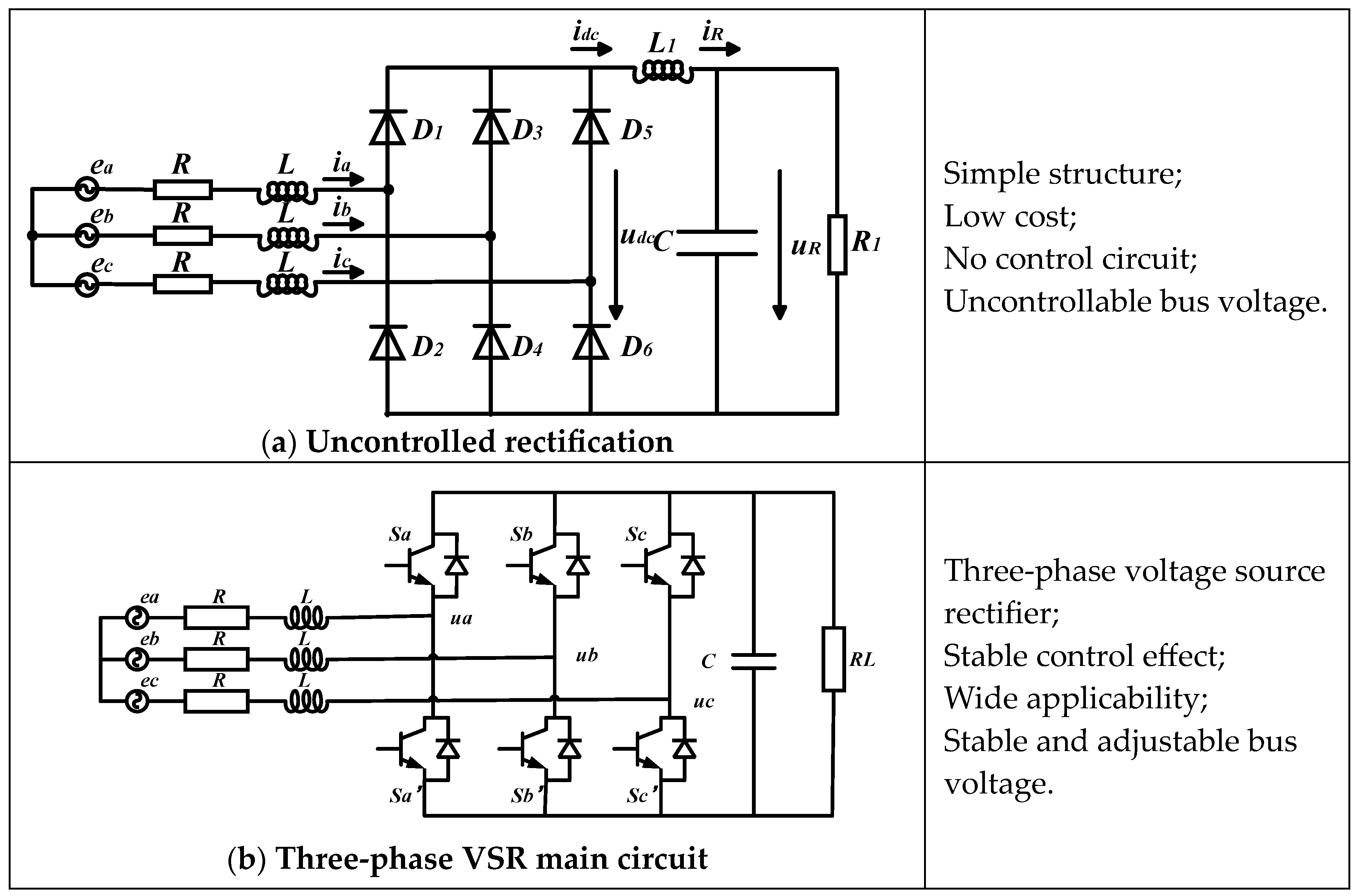
3.1. Uncontrolled Rectification

As illustrated in Figure 9, a comparison is made between the topological structures of three-phase uncontrolled rectification and three-phase VSR-based controlled rectification. The three-phase electric power generated by the FPLG system, after processing by rectification diodes, can output DC power in an open-loop control manner, with the bus voltage magnitude determined by the DC terminal resistance. In contrast, the three-phase VSR-based controlled rectification employs a dual closed-loop control strategy to achieve a stable and adjustable bus voltage.

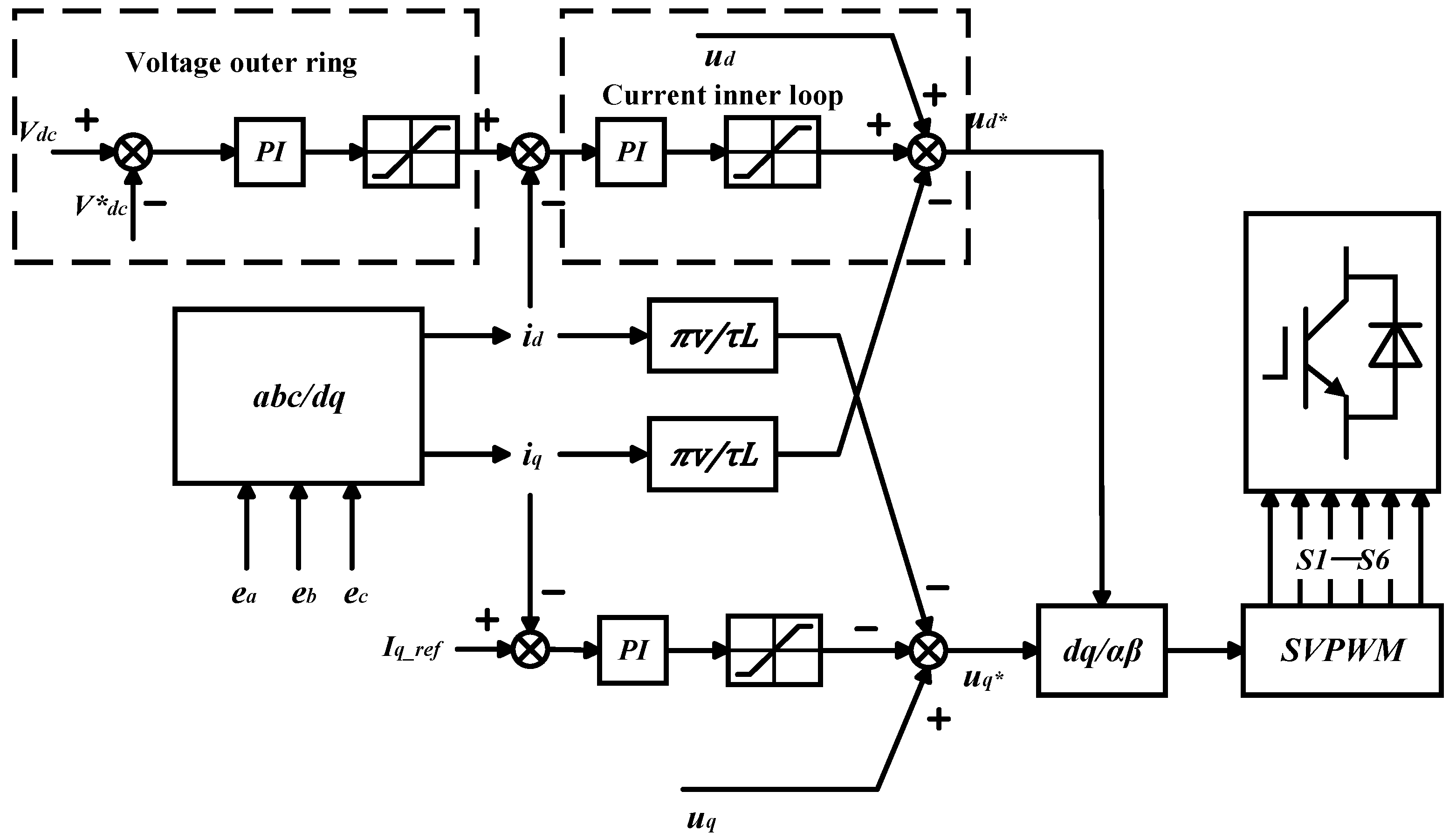
3.2. PWMC Rectification Control Strategy

In the free-piston internal combustion linear power generation system, the free piston’s motion curve is sine-like. Consequently, the mover’s velocity in the linear motor and the resulting three-phase voltage and current can be approximated as sine waves. This allows the electric power output from the linear motor to be processed using PWMC, which also regulates the electromagnetic force in the linear motor, enhancing the system’s stability and reliability.

PWMC rectification strategies are categorized into three-phase voltage-source rectification (VSR) and current-source rectification (CSR) based on the main circuit type. Compared to CSR, VSR is more straightforward and offers highly controllable output voltage and frequency, making it more adaptable to the linear generator’s varying amplitude and frequency characteristics. Hence, this study adopts the three-phase VSR strategy for motor power rectification.

The dual-loop control block diagram of the system is shown in Figure 10. The rectification system adopts a dual-loop control structure, which is formed by a voltage outer loop and a current inner loop based on PI control. The voltage outer loop is used to regulate the DC bus capacitance voltage to stabilize it at the target value. The output of the voltage outer loop control compensator serves as the reference value for the current inner loop. By adjusting the machine-side current, the current inner loop ensures that the voltage and current phases are the same and that the machine-side current stably follows the reference current. This enables the rectifier to operate stably.

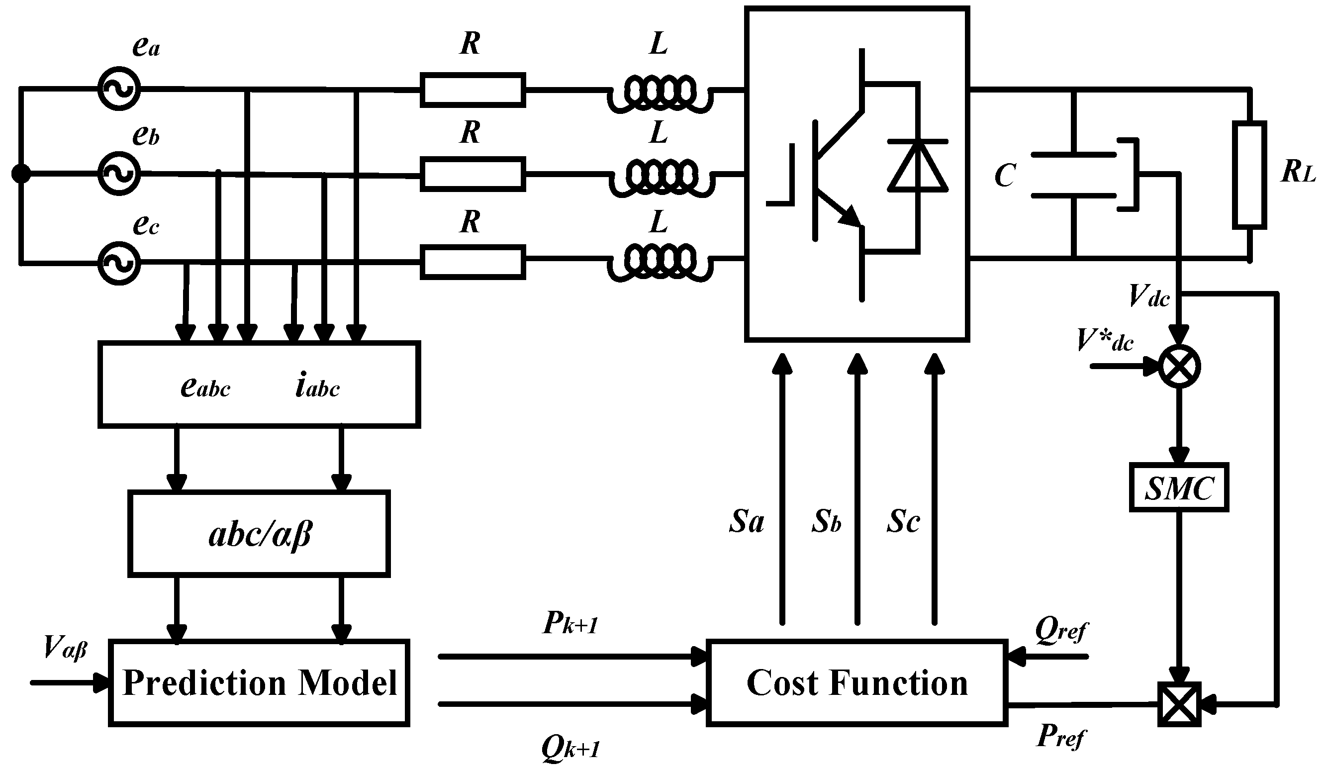
3.3. MPSMC Control Strategy

Traditional PWMC dual-loop control has drawbacks such as slow dynamic response, weak anti-interference capability, and complex parameter tuning. To address these issues, this paper proposes a model predictive sliding mode compound control strategy. Model predictive control (MPC), a discrete sampling control method, uses rolling optimization to mitigate the impact of uncertainties like model mismatch, distortion, and disturbances. This ensures better control performance. However, MPC has limitations, including computationally intensive algorithms and slow dynamic response due to PI control in the outer loop. To enhance system robustness, a sliding mode controller replaces the PI control in the voltage outer loop, reducing the algorithm’s optimization iterations.

The current inner loop employs MPC with online rolling optimization to minimize the impact of uncertainties, achieving better control performance. The voltage outer loop uses a sliding mode controller instead of PI control to shorten the optimization process and improve robustness. This compound control strategy effectively combines the strengths of MPC and sliding mode control, offering enhanced dynamic response and anti-interference capability while maintaining stable voltage regulation.

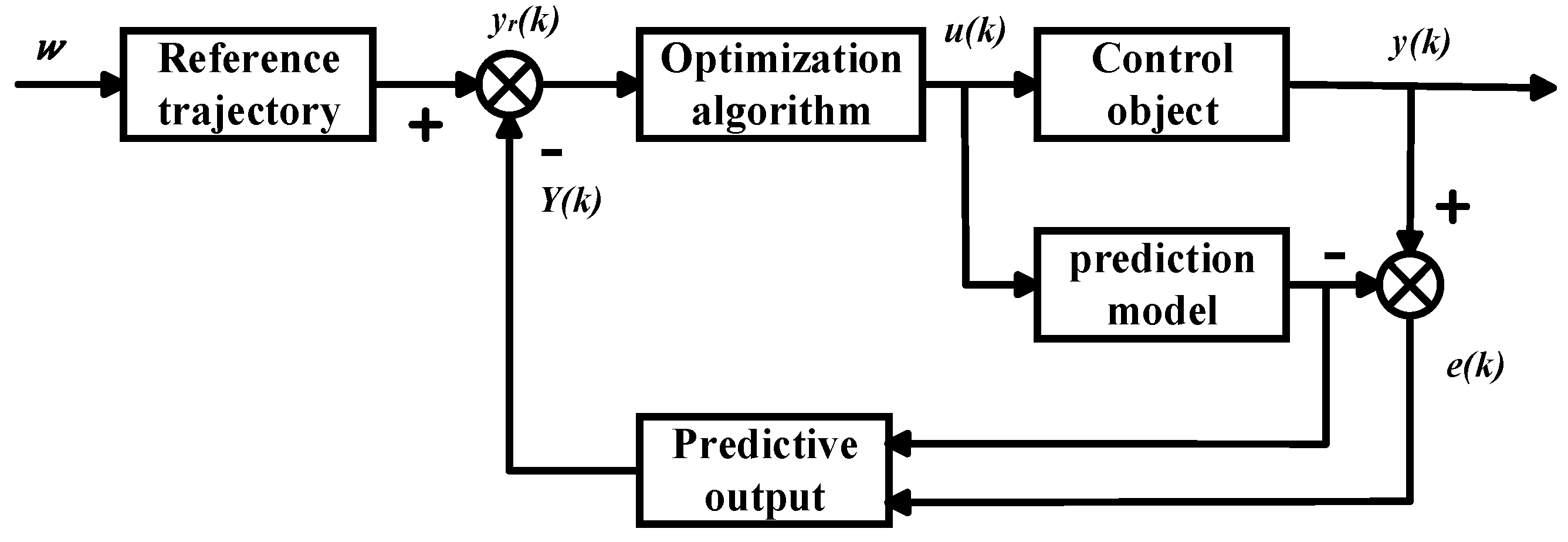
3.3.1. Design of Model Predictive Controller

The principle of model predictive control is shown in Figure 11, and its basic process is:

(1)

Establish a predictive model. Establish a predictive model based on the current system model and predict the future state of the system based on its current state.

(2)

Perform rolling optimization. Build a suitable cost function to determine the best control quantity for upcoming systems.

(3)

System feedback correction. Model predictive control can provide feedback correction for errors based on the current state of system.

The model predictive control-based rectification strategy’s main process is shown in Figure 12.

In the control strategy of three-phase controlled rectification, coupling occurs between the d-axis current and q-axis current. To better design the model predictive control loop, the mathematical equations of the current loop need to be rewritten as follows:

$$\left\{\begin{array}{c}{\displaystyle \frac{d{i}_d}{dt}}=-{\displaystyle \frac{R}{L}}{i}_d+{\displaystyle \frac{U_d}{L}}\\ {\displaystyle \frac{d{i}_q}{dt}}=-{\displaystyle \frac{R}{L}}{i}_q+{\displaystyle \frac{U_q}{L}}\end{array}\right.$$

(8)

In the formula, $R$ is the resistance of the coil in the linear motor, $L$ is the inductance in the linear motor, assuming a sampling period of $T_s$,

Among them, $U_d$ and $U_q$ are the voltage drops on the $dq$ axis of the linear motor coil, which can be expressed as:

$$\left\{\begin{array}{c}{U}_d=e_d-V_d+\omega L{i}_q\\ U_q=e_q-V_q-\omega L{i}_d\end{array}\right.$$

(9)

In the formula, $V_d$ and $V_q$ represent the components along the $dq$ axis on the AC side of the linear motor, which can be expressed as:

$$\left\{\begin{array}{c}{V}_d=U_{dc}\cdot S_d\\ V_q=U_{dc}\cdot S_q\end{array}\right.$$

(10)

Based on the above analysis, the above equation is rewritten into discrete form.

$$\left\{\begin{array}{c}{i}_d\left(k+1\right)=\left(1-R{\displaystyle \frac{T_S}{L}}\right)i_d\left(k\right)+{\displaystyle \frac{T_S}{L}}{U}_d\left(k\right)\\ i_q\left(k+1\right)=\left(1-R{\displaystyle \frac{T_S}{L}}\right)i_q\left(k\right)+{\displaystyle \frac{T_S}{L}}{U}_q\left(k\right)\end{array}\right.$$

(11)

Given a prediction interval length of $L_P$, taking the $I_d$ component as an example, the current expression within the prediction interval is:

$$\left[\begin{array}{c}{\widehat{i}}_d\left(k+1\right)\\ {\widehat{i}}_d\left(k+2\right)\\ ⋮\\ {\widehat{i}}_d\left(k+L_p\right)\end{array}\right]=\left[\begin{array}{c}1-{\displaystyle \frac{R{T}_s}{L}}\\ {\left(1-{\displaystyle \frac{R{T}_s}{L}}\right)}^2\\ ⋮\\ {\left(1-{\displaystyle \frac{R{T}_s}{L}}\right)}^{L_p}\end{array}\right]i_d\left(k\right)+\left[\begin{array}{cccc}{\displaystyle \frac{T_s}{L}}& 0& \cdots & 0\\ \left(1-{\displaystyle \frac{R{T}_s}{L}}\right){\displaystyle \frac{T_s}{L}}& {\displaystyle \frac{T_s}{L}}& \cdots & 0\\ ⋮& ⋮& \ddots & ⋮\\ {\left(1-{\displaystyle \frac{R{T}_s}{L}}\right)}^{i-1}{\displaystyle \frac{T_s}{L}}& {\left(1-{\displaystyle \frac{R{T}_s}{L}}\right)}^{i-2}{\displaystyle \frac{T_s}{L}}& \cdots & {\displaystyle \frac{T_s}{L}}\end{array}\right]\left[\begin{array}{c}{U}_d\left(k\right)\\ U_d\left(k+1\right)\\ ⋮\\ U_d\left(k+L_p-2\right)\end{array}\right]$$

(12)

To ensure stable and adjustable output voltage while maintaining good system control performance, model predictive control must incorporate output constraints. Consequently, its cost function is formulated as follows:

$$J=\sum {\left[y\left(k+i\right)-\omega \left(k+i\right)\right]}^{2}Q\left(i\right)+\sum {\left[u\left(k+j-1\right)\right]}^2\lambda \left(j\right)$$

(13)

In the formula, $Q_i$ and ${\lambda }_j$ represent error weighting coefficients and control weighting coefficients respectively; $Y_i$ and ${\omega }_i$ represent the actual input and expected input of the controller respectively; $L_u$ represents the length of the control interval, $J$ is the cost function, and is the optimization objective function of the MPSMC algorithm. The relevant switch vector is found and applied to the rectifier bridge by using the cost function’s minimization as the goal to obtain a precise control effect.

Rewrite the above equation into a matrix expression as follows:

$$J={\left(Y-W\right)}^T\overline{Q}\left(Y-W\right)+U^T\overline{R}U$$

(14)

In the formula, $W$ is the expected input vector of the controller; $Y$ is the actual input vector of the controller; $U$ is the output vector of the controller; $Q$ and $R$ are control matrices, respectively. The specific components can be represented as follows:

$$\left\{\begin{array}{l}W={\left(\begin{array}{cccc}{i}_{dref}\left(k+1\right)& i_{dref}\left(k+2\right)& \dots & i_{dref}\left(k+L_p\right)\end{array}\right)}^T\\ Y={\left(\begin{array}{cccc}{i}_d\left(k+1\right)& i_d\left(k+2\right)& \dots & i_d\left(k+L_p\right)\end{array}\right)}^T\\ U={\left(\begin{array}{cccc}{i}_q\left(k+1\right)& i_q\left(k+2\right)& \dots & i_q\left(k+L_p\right)\end{array}\right)}^T\end{array}\right.$$

(15)

In model predictive control of the current inner loop, sampling time is chosen based on system requirements and computational capability. For the fast—response system in this paper, the prediction horizon is set to 2–3 sampling periods to balance prediction accuracy and computational complexity. Control gain is adjusted and optimized via simulation to achieve desired overshoot and settling time. The weighting matrix is determined by assigning weights to different terms in the objective function, with reasonable values obtained through simulation analysis to ensure optimal control performance.

Based on the aforementioned analysis, the design of the model predictive control current loop can be accomplished. The current loop is designed to regulate the machine-side current, ensuring that the voltage and current on the machine side are in phase. Additionally, it stabilizes the current value at the desired level.

3.3.2. Design of Sliding Mode Controller

Traditional control systems depend on PI controllers for setting active power references in the outer loop, employing linear control strategies. Nevertheless, when system parameters or operating conditions vary, the control effectiveness under such strategies is subpar. In comparison, sliding mode control is better equipped to handle nonlinear systems. Once the controller attains the sliding surface, its sensitivity to system parameters diminishes. Hence, to significantly enhance control effectiveness, the outer-loop controller is substituted with a sliding mode controller.

According to the law of conservation of energy, the input power of a rectifier should equal its output power. For simplicity, this paper ignores any power loss during rectifier operation.

$$P=V_{\mathrm{dc}}{i}_{\mathrm{dc}}=C{V}_{\mathrm{dc}}{\displaystyle \frac{d}{dt}}{V}_{\mathrm{dc}}+{\displaystyle \frac{1}{R_L}}{V}_{\mathrm{dc}}^2$$

(16)

In order to achieve precise tracking of the output voltage to the expected voltage value, a tracking error $e$ will be defined, which is used to measure the deviation between the output voltage and the expected voltage.

$$e=V_{\mathrm{dc}}^{*}-V_{\mathrm{dc}}$$

(17)

To achieve zero steady-state error, a proportional-integral sliding surface for voltage error is designed using the sliding mode variable structure control principle.

$$s=c_{1}e+c_2\int edt$$

(18)

In the formula, c₁ > 0, c₂ > 0, taking the derivative of the sliding surface, is obtained by substituting the above formula.

$$\dot{s}=-c_1\left({\displaystyle \frac{P}{C{V}_{\mathrm{dc}}}}-{\displaystyle \frac{V_{\mathrm{dc}}}{R_{L}C}}\right)+c_2\left(V_{\mathrm{dc}}^{*}-V_{\mathrm{dc}}\right)$$

(19)

To enhance the efficiency and performance of the system in reaching the sliding mode, a fast power reaching law was employed in the design of the voltage outer-loop controller.

$$\dot{s}=-k_{1}s-k_2|s{|}^{\alpha }\mathit{sgn}(s)$$

(20)

In the formula, k₁ > 0, k₂ > 0, 0 < α, the sgn is a signed function passed through α. It is ensured that when the system state moves away from the sliding mode surface, it can swiftly approach the sliding mode to accelerate the convergence speed by using a fast power-law approach law. As the system state gradually approaches the sliding mode surface, reducing the control gain can effectively reduce the chattering phenomenon and achieve a smoother transition.

By combining the above equations, we can obtain:

$$\begin{array}{c}{k}_{1}s+k_2|s{|}^{\alpha }\mathit{sgn}(s)-c_1{\displaystyle \frac{P}{C{V}_{\mathrm{dc}}}}+c_1{\displaystyle \frac{V_{\mathrm{dc}}}{R_{L}C}}+\\ c_2\left(V_{\mathrm{dc}}^{*}-V_{\mathrm{dc}}\right)=0\end{array}$$

(21)

Further conversion:

$$P_{\mathrm{ref}}={\displaystyle \frac{C{V}_{\mathrm{dc}}}{c_1}}\left(k_{1}s+k_2|s{|}^{\alpha }\mathit{sgn}(s)+{\displaystyle \frac{c_1{V}_{\mathrm{dc}}}{R_{L}C}}+c_{2}e\right)$$

(22)

The control law and reference power Pref of the sliding mode controller were obtained using the above formula. Given the complex operating conditions that three-phase rectifiers may face in actual operation, in order to reduce chattering, the saturation function $sat (s)$ was adopted to replace the discontinuous sign function $sgn (s)$.

Replacing the sign function $sgn (s)$ with a saturation function $sat (s)$ can significantly reduce chattering in sliding mode control, thereby enhancing system stability. This substitution introduces a boundary layer to smooth the control input, avoiding the abrupt changes that occur when the sign function switches.

$$sat(s)=\left\{\begin{array}{c}\begin{array}{cc}1& s>\mathsf{\Delta }\end{array}\\ \begin{array}{cc}{\displaystyle \frac{s}{\mathsf{\Delta }}}& |s|\ge \mathsf{\Delta }\end{array}\\ \begin{array}{cc}-1& s<-\mathsf{\Delta }\end{array}\end{array}\right.$$

(23)

In the formula, Δ is the thickness of the boundary layer and Δ > 0. After replacing the switch function, the above equation can be rewritten as:

$$P_{\mathrm{ref}}={\displaystyle \frac{C{V}_{\mathrm{dc}}}{c_1}}\left(k_{1}s+k_2|s{|}^{\alpha }sat(s)+{\displaystyle \frac{c_1{V}_{\mathrm{dc}}}{R_{L}C}}+c_{2}e\right)$$

(24)

To enhance system responsiveness and ensure an adjustment time within 0.2, appropriate sliding—mode controller parameters must be calculated. This requires considering system characteristics and control objectives. In this paper, a suitable sliding surface is constructed. The Lyapunov method is used for control effect analysis to determine parameter ranges. Also, the impact of disturbances and uncertainties is considered. Afterward, parameters are optimized.

A necessary precondition for constructing sliding mode control is the existence of the sliding mode. We must rigorously verify the existence conditions of its sliding mode in order to guarantee that the trajectory points near the sliding surface can successfully reach the sliding surface in a finite amount of time.

Select the Lyapunov function as:

$$V={\displaystyle \frac{1}{2}}{s}^2$$

(25)

By performing deformation treatment on the above equation, it can be concluded that:

$$\dot{V}=s\dot{s}=-k_1{s}^2-k_{2}s|s{|}^{\alpha }sat(s)$$

(26)

If the arrival point is in a positive position within the field of the created switch surface, s > 0. There are:

$$sat(s)=\left\{\begin{array}{c}\begin{array}{cc}1& s>\mathsf{\Delta }\end{array}\\ \begin{array}{cc}{\displaystyle \frac{s}{\mathsf{\Delta }}}& |s|\le \mathsf{\Delta }\end{array}\end{array}\right.$$

(27)

$$\dot{V}=-k_1{s}^2-k_{2}s|s{|}^{\alpha }sat(s)<-k_{2}s|s{|}^{\alpha }sat(s)<0$$

(28)

If the arrival point is in a negative position within the field of the created switch surface, i.e., s < 0. There are:

$$sat(s)=\left\{\begin{array}{c}\begin{array}{cc}{\displaystyle \frac{s}{\mathsf{\Delta }}}& |s|\ge \mathsf{\Delta }\end{array}\\ \begin{array}{cc}-1& s<-\mathsf{\Delta }\end{array}\end{array}\right.$$

(29)

$$\dot{V}=-k_1{s}^2-k_{2}s|s{|}^{\alpha }sat(s)<k_{2}s|s{|}^{\alpha }<0$$

(30)

From the above analysis, it can be concluded that the existing sliding mode condition is satisfied.

The final control block diagram of the Model Predictive Sliding Mode Control (MPSMC) is shown in Figure 13, where the voltage outer loop employs a sliding mode controller, while the current inner loop utilizes a model predictive controller.

4. Evaluation of Electric Energy Output Quality

This paper compares and examines the robustness, accuracy, and responsiveness of the three rectification methods after finishing the theoretical modeling analysis previously indicated. The comparison’s outcomes are displayed below.

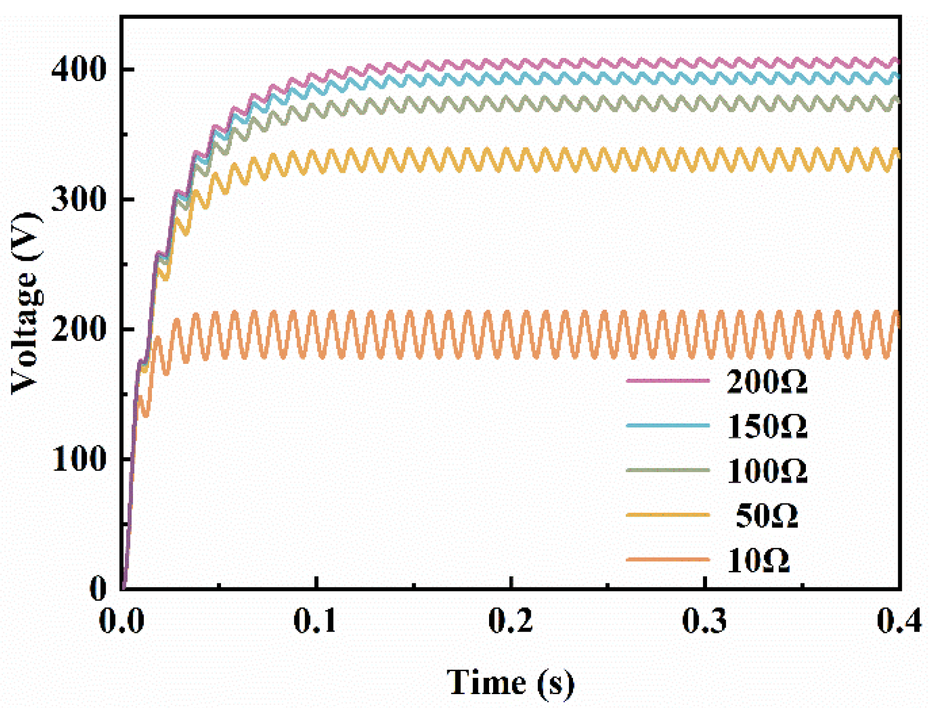
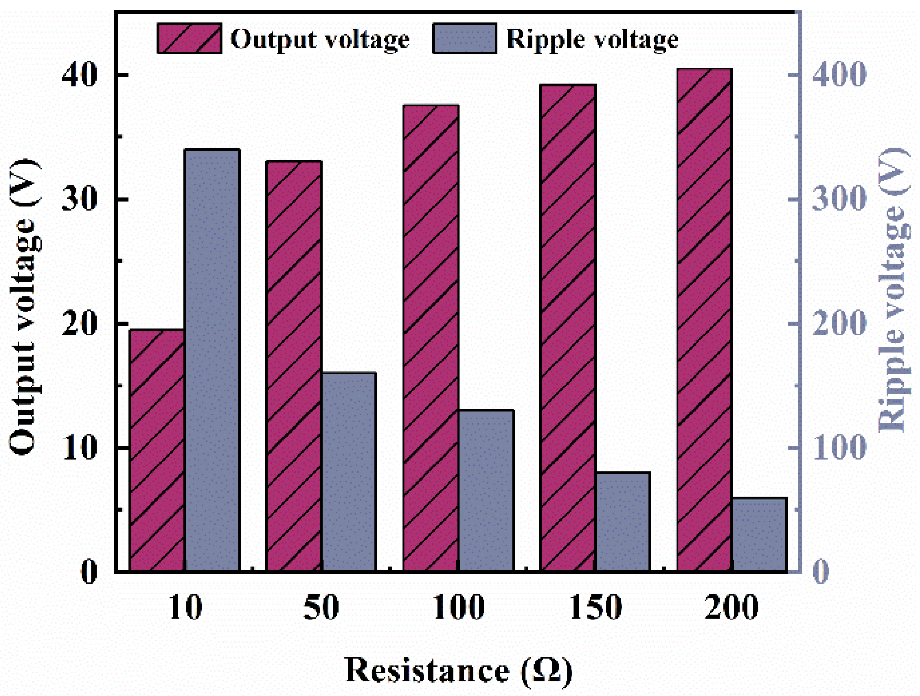
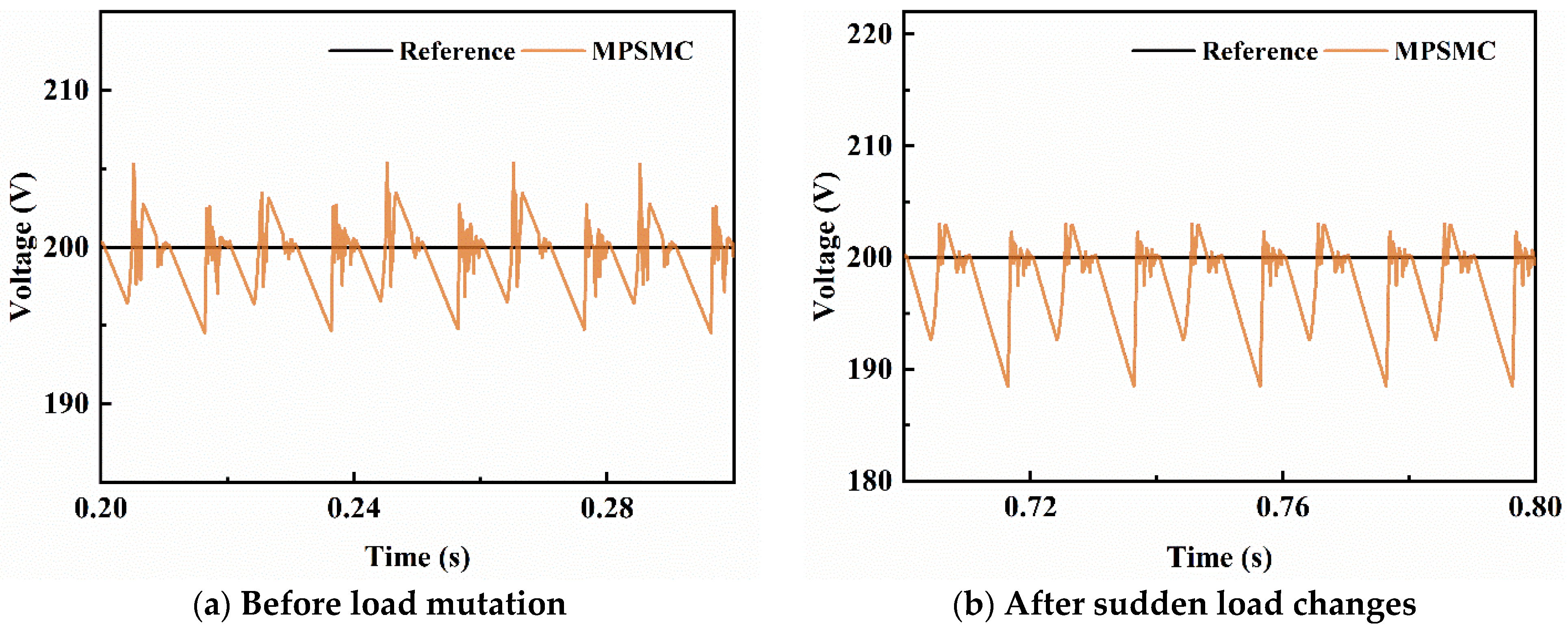
4.1. Robustness Analysis

(1)

Uncontrolled rectification

Under the uncontrolled rectification strategy, the entire circuit uses open-loop control. The output voltage at the load end is entirely determined by the load characteristics, as the three-phase electric power is processed solely by the unidirectional conductivity of diodes. In this paper, an uncontrolled rectification model is established based on the aforementioned analysis of three-phase uncontrolled rectification. Simulation tests are conducted under different load resistance values (10 Ω, 50 Ω, 100 Ω, 150 Ω, and 200 Ω). The test results are shown in Figure 14. Figure 15 shows that the output voltage at the load end increases with growing load resistance, but the rate of increase slows down. Once the resistance reaches a certain level, the output voltage stabilizes and ceases to rise. This is attributed to the limitations of the linear motor’s stroke and frequency, which prevent the output voltage from rising indefinitely.

Under identical motor parameters, electrical parameters of the main circuit, connection methods, and load characteristics, a load mutation test was performed on the rectification system. The linear motor operated at 50 Hz with an 80 mm mover stroke. The load resistance mutated from 150 Ω to 75 Ω at 0.5 s. Simulation results are shown in Figure 16. At startup, the load-end output voltage was about 390 V and stabilized in approximately 0.15 s. Upon load mutation, the FPLG system exhibited prolonged fluctuations, taking around 0.4 s to restabilize. The output voltage fluctuated significantly. At 75 Ω, the output voltage was about 340 V. The uncontrolled rectification scheme caused substantial voltage fluctuations, indicating room for improvement in power quality.

Using the uncontrolled rectification strategy can cause serious current disruptions in the three-phase current output from the linear motor. Figure 17 shows the three-phase current data of the linear motor collected during the simulation. In the three-phase rectifier circuit, each phase current on the AC side undergoes two conduction processes within a half-cycle, resulting in discontinuous and continuous phase currents. Under uncontrolled rectification, the current periodic work time ratio is only about 50%, which significantly reduces the motor’s output efficiency.

(2)

Robustness analysis of PWMC rectification and MPSMC rectification results

This paper has presented the rectification principle based on MPSMC control, investigated the feasibility of applying the model predictive control strategy to the linear internal combustion power generation system, and established a simulation platform using Matlab/Simulink. Given that the sampling period, control horizon, and prediction horizon all influence control performance, the sampling period was set at 0.0002 s. The simulation results are as follows:

A load mutation test was carried out on the MPSMC controller designed in this study while keeping the motor parameters, main—circuit electrical parameters, circuit connections, and load characteristics identical. The load voltage was maintained at 200 V. At 0.5 s, the load resistance was stepped down from 100 Ω to 50 Ω. The simulation results for the load voltage and current waveforms are presented in Figure 18, Figure 19 and Figure 20.

Figure 18 shows that under MPSMC control, the load voltage stabilizes at the reference value in just 35 ms. After a load mutation at 0.5 s, the system responds in only 80 ms, highlighting the controller’s robustness. As depicted in Figure 19, the output voltage remains stable near the reference value with a 20 ms system response time and a 7% overshoot, indicating minimal voltage fluctuation. The DC-end current control effectiveness is also verified. Ohm’s law suggests the load current should step from 2 A to 4 A, and the simulation results in Figure 20 confirm this, showing minimal current fluctuation. Overall, the MPSMC control strategy demonstrates excellent performance under voltage mutations.

The following figure illustrates the dynamic response of the system under MPSMC control and PWMC control. As depicted in Figure 21 and Figure 22, when the reference voltage changes at 0.5 s, both control strategies eventually stabilize the output voltage at the desired value. This indicates that both strategies exhibit good dynamic response and that the system can accommodate a wide range of load variations. While the PWMC-controlled system stabilizes approximately 0.25 s after the load mutation, the MPSMC-controlled system reaches stability in only 0.08 s after the load mutation. This demonstrates the superior performance of MPSMC control compared to PWMC control.

As can be seen from the simulation results of the two control methods, the peak time and rise time of the DC bus voltage under both MPSMC and PWMC control are similar. However, the MPSMC controller shows a significant reduction in maximum overshoot and settling time. This indicates that the MPSMC controller has better responsiveness and robustness.

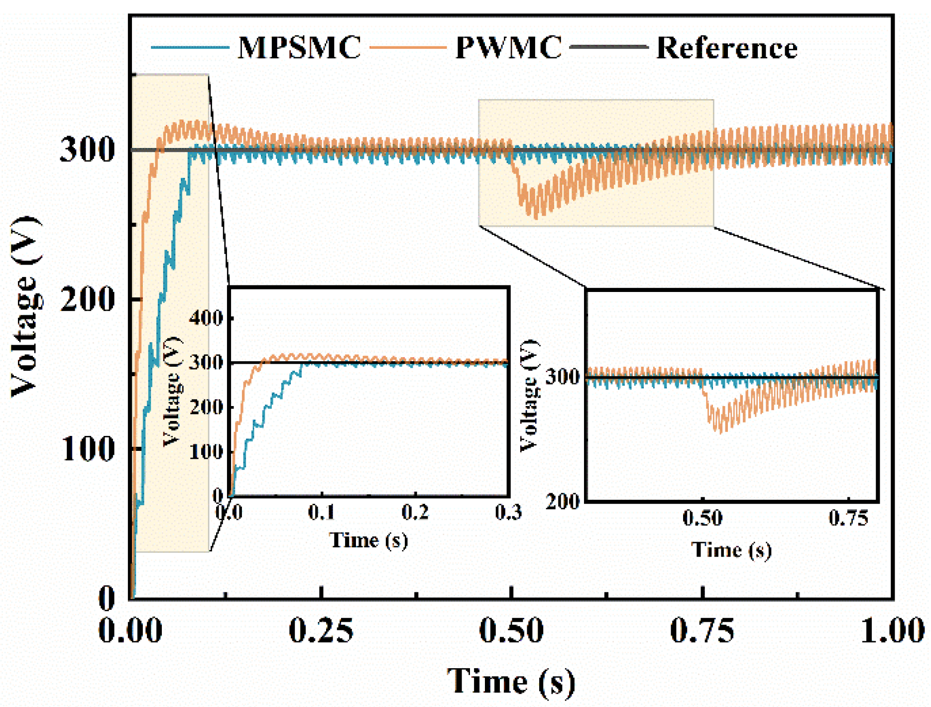
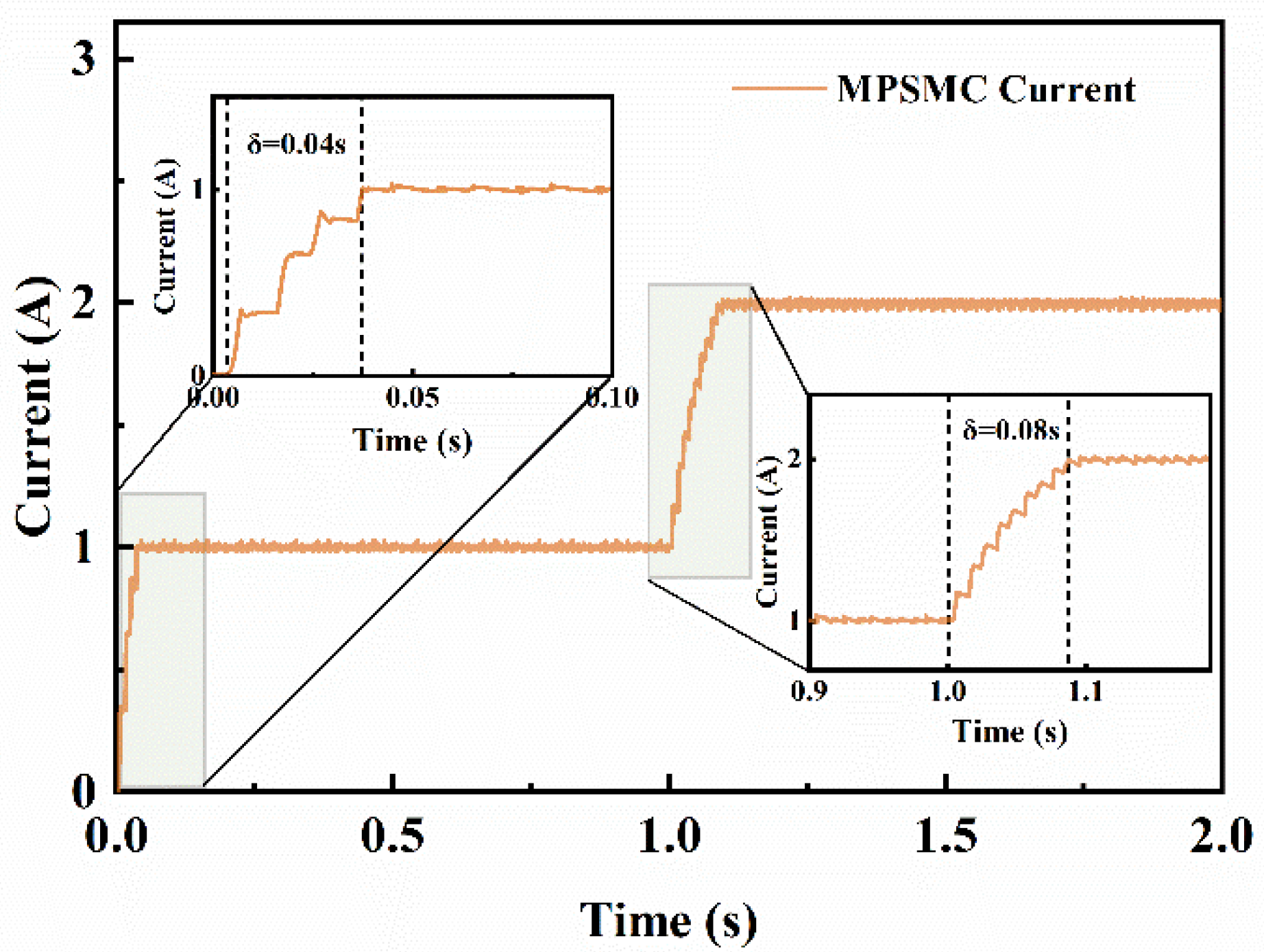
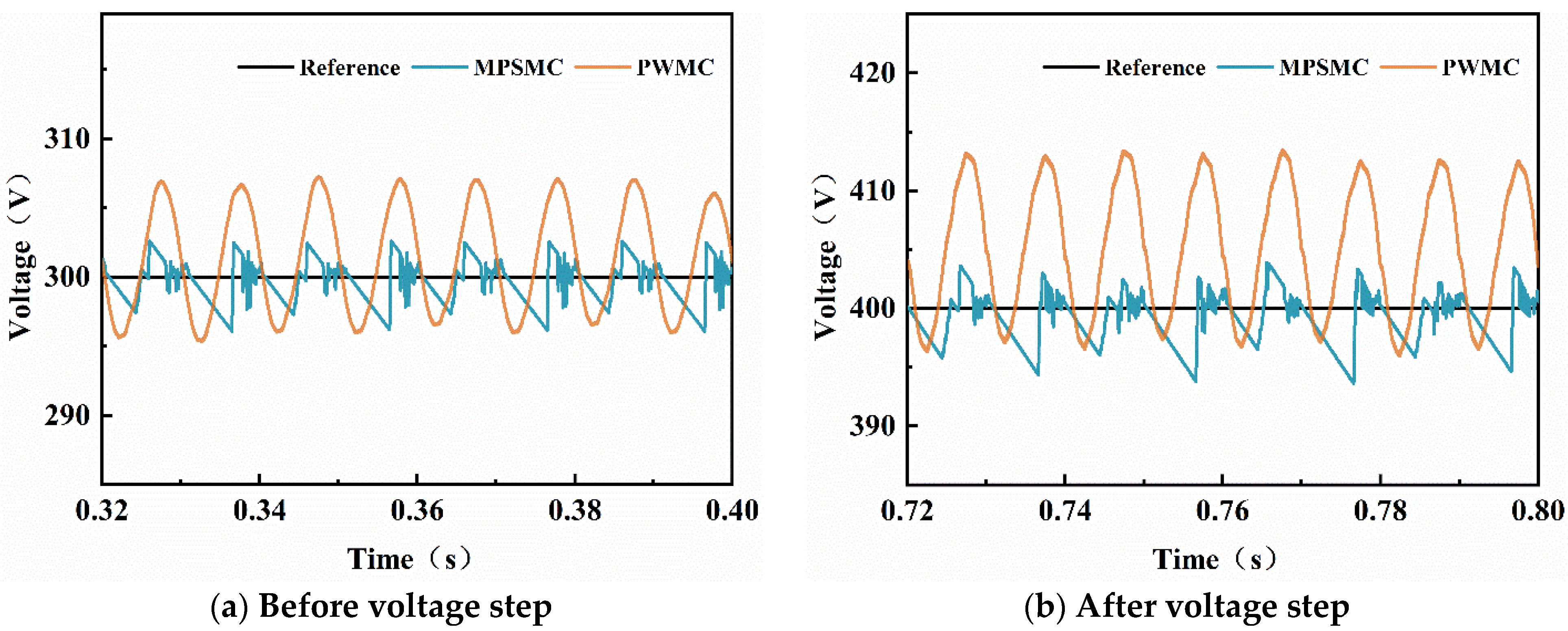
4.2. Analysis of Responsiveness and Accuracy

The designed MPSMC controller was tested via a voltage step test under identical motor parameters, main—circuit electrical parameters, circuit connections, and load characteristics. Load resistance was 200 Ω, and the bus voltage stepped from 200 V to 400 V at 1 s. Simulation yielded load—end voltage and current waveforms as shown in Figure 23.

As indicated in Figure 23, the load-end bus voltage remains stable at the set value under MPSMC control, highlighting the effectiveness of the voltage outer loop in the control strategy.When a step signal is issued at 1s, the system responds promptly with a response time of only 80 ms, demonstrating the controller’s robustness. Under MPSMC control, when the set voltage is 200 V, the peak voltage at the DC terminal reaches approximately 205 V, resulting in an overshoot of about 3.5%. This indicates that the output voltage remains relatively stable. The MPSMC controller exhibits strong anti-interference capabilities, effectively reducing voltage impacts on system components and ensuring stable FPLG system operation. Moreover, the control strategy effectively regulates the current at the DC terminal. As shown in Figure 24, when the voltage steps from 200 V to 400 V under purely resistive load conditions with a resistance of 200 Ω, the current at the load end is expected to step from 1 A to 2 A. Comparing the simulation results with the expected values confirms the accuracy of the control strategy and shows that the output current remains stable with minimal fluctuations. This further underscores the MPSMC control strategy’s effectiveness in maintaining system stability during voltage mutations.

This paper compares the control effectiveness of MPSMC and PWMC and assesses their dynamic responses through voltage step tests. At 0.5 s, the output voltage steps from 300 V to 400 V. Simulation results in Figure 25 and Figure 26 show that both strategies stabilize the output voltage quickly. Under PWMC, the output voltage initially overshoots to about 330 V and stabilizes in 120 ms. In contrast, the MPSMC-controlled system stabilizes in just 70 ms with less voltage fluctuation, highlighting its superior robustness.

When the voltage step occurs at 0.5 s, both strategies quickly restabilize the output voltage near the set value. However, the MPSMC-controlled system achieves stability more rapidly. The output voltage under MPSMC has a peak of 303 V with a 4.3% overshoot, compared to 308 V and a 10% overshoot under PWMC. This demonstrates that MPSMC effectively reduces bus voltage peaks and minimizes the impact of voltage fluctuations on electrical components. The output voltage waveform under MPSMC is also smoother, indicating higher power quality. Additionally, under the same conditions, the DC bus voltage ripple is lower with MPSMC control than with PWMC control.

5. Conclusions

This paper explores rectification strategies with different control algorithms for the free-piston internal combustion linear power generation system. Aiming to handle the output characteristics of the linear motor within the system, it delves into three strategies: uncontrolled rectification, PWM rectification with PI control, and a compound strategy combining model predictive control and sliding mode control. The key conclusions are as follows:

(1)

Uncontrolled rectification can convert three-phase AC to DC, but due to open-loop control, the output DC voltage is uncontrollable and fluctuates greatly, influenced by the linear motor’s characteristics.

(2)

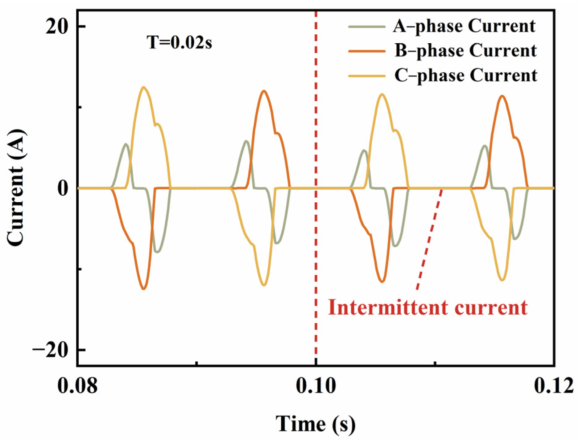
Uncontrolled rectification will cause serious current disruption in the linear motor side of the system.

(3)

Model predictive sliding mode compound control enhances the system’s anti-interference capability. Compared to traditional PWM rectification, it offers faster response, better robustness, lower bus voltage ripple, and superior power quality.

(4)

Model predictive control and sliding mode control are nonlinear control methods. They adapt better in nonlinear settings like free-piston internal combustion linear power generation systems.

References

1. Leick, M.T.; Moses, R.W. Experimental Evaluation of the Free Piston Engine-Linear Alternator (FPLA); Sandia National Lab: Albuquerque, NM, USA, 2015.
2. Zheng, J.; Chen, J.; Zheng, P.; Wu, H.; Tong, C. Research on control strategy of free piston Stirling power generating system. Energies 2017, 10, 1609. [Google Scholar] [CrossRef]
3. Li, J.; Zuo, Z.; Liu, W.; Jia, B.; Feng, H.; Wang, W.; Smallbone, A.; Roskilly, A.P. Generating performance of a tubular permanent magnet linear generator for application on free-piston engine generator prototype with wide-ranging operating parameters. Energy 2023, 278, 127851. [Google Scholar] [CrossRef]
4. Chen, J.; Liao, Y.; Zhang, C.; Jiang, Z. Design and analysis of a permanent magnet linear generator for a free-piston energy converter. In Proceedings of the 2014 9th IEEE Conference on Industrial Electronics and Applications, Hangzhou, China, 9–11 June 2014; pp. 1719–1723. [Google Scholar]
5. Gong, X.; Zaseck, K.; Kolmanovsky, I.; Chen, H. Modeling and predictive control of free piston engine generator. In Proceedings of the 2015 American Control Conference (ACC), Chicago, IL, USA, 1–3 July 2015; pp. 4735–4740. [Google Scholar]
6. Moriya, K.; Goto, S.; Akita, T.; Kosaka, H.; Hotta, Y.; Nakakita, K. Development of Free Piston Engine Linear Generator System Part3-Novel Control Method of Linear Generator for to Improve Efficiency and Stability; SAE Technical Paper; SAE: Warrendale, PA, USA, 2016. [Google Scholar]
7. Lin, J.; Xu, Z.; Chang, S.; Yan, H. Finite-time thermodynamic modeling and analysis of an irreversible Miller cycle working on a four-stroke engine. Int. Commun. Heat Mass Transf. 2014, 54, 54–59. [Google Scholar] [CrossRef]
8. Kock, F.; Haag, J.; Friedrich, H.E. The Free Piston Linear Generator-Development of an Innovative, Compact, Highly Efficient Range-Extender Module; SAE Technical Paper; SAE: Warrendale, PA, USA, 2013. [Google Scholar]
9. Raheem, A.T.; Aziz, A.R.A.; Zulkiffi, S.A.; Rahem, A.T.; Ayandotun, W.B. A review of free piston engine control literature—Taxonomy and techniques. Alex. Eng. J. 2022, 61, 7877–7916. [Google Scholar] [CrossRef]
10. Chen, C.; Tong, C.; Liu, B.; Zheng, P.; Jing, S. Trajectory-Regulation-Based Segmented Control for Dead Center Positions Tracking of Free-Piston Linear Generator. IEEE Trans. Ind. Electron. 2022, 70, 3426–3436. [Google Scholar] [CrossRef]
11. Vu, D.N.; Lim, O. Piston motion control for a dual free piston linear generator: Predictive-fuzzy logic control approach. J. Mech. Sci. Technol. 2020, 34, 4785–4795. [Google Scholar] [CrossRef]
12. Raheem, A.T.; Aziz, A.R.A.; Zulkiffi, S.A.; Baharom, M.B.; Rahem, A.T.; Ayandotun, W.B. Optimisation of operating parameters on the performance characteristics of a free piston engine linear generator fuelled by CNG–H2 blends using the response surface methodology (RSM). Int. J. Hydrogen Energy 2022, 47, 1996–2016. [Google Scholar] [CrossRef]
13. Ayandotun, W.B.; Aziz, A.R.A.; Karim, Z.A.A.; Mohammed, S.E.; Raheem, A.T.; Ismael, M.A. Investigation on the combustion and performance characteristics of a DI free piston linear generator engine fuelled with CNG-CO2 blend. Appl. Therm. Eng. 2021, 198, 117441. [Google Scholar] [CrossRef]
14. Zhang, F.; Chen, G.; Wu, D.; Li, T.; Zhang, Z.; Wang, N. Characteristics of ammonia/ hydrogen premixed combustion in a novel Linear Engine Generator. Multidiscip. Digit. Publ. Inst. Proc. 2020, 58, 2. [Google Scholar]
15. Ismael, M.A.; Aziz, A.R.A.; Mohammed, S.E.; Baharom, M.B.; Ibrahim, M.H.; Sahalan, M.; Qawiy, A. Effect of aspect ratio on frequency and power generation of a free-piston linear generator. Appl. Therm. Eng. 2021, 192, 116944. [Google Scholar]
16. Sato, M.; Naganuma, K.; Nirei, M.; Yamanaka, Y.; Suzuki, T.; Goto, T.; Bu, Y.; Mizuno, T. Improving the constant-volume degree of combustion considering generatable range at low speed in a free-piston engine linear generator system. IEEJ Trans. Electr. Electron. Eng. 2019, 14, 1703–1710. [Google Scholar] [CrossRef]
17. Feng, H.; Zhang, Z.; Jia, B.; Zuo, Z.; Smallbone, A.; Roskilly, A.P. Investigation of the optimum operating condition of a dual piston type free piston engine generator during engine cold start-up process. Appl. Therm. Eng. 2021, 182, 116124. [Google Scholar] [CrossRef]
18. Li, X.; Sun, Y.; Wang, H.; Su, M.; Huang, S. A hybrid control scheme for three-phase Vienna rectifiers. IEEE Trans. Power Electron. 2017, 33, 629–640. [Google Scholar] [CrossRef]
19. Tai, L.; Lin, M.; Li, H.; Li, Y. A novel three-vector-based model predictive direct power control for three-phase PWM rectifier. Electronics 2021, 10, 2579. [Google Scholar] [CrossRef]
20. Fu, C.; Zhang, C.; Zhang, G.; Song, J.; Zhang, C.; Duan, B. Disturbance observer-based finite-time control for three-phase AC–DC converter. IEEE Trans. Ind. Electron. 2021, 69, 5637–5647. [Google Scholar] [CrossRef]
21. Wang, W.; Yin, H.; Guan, L. Parameter setting for double closed-loop vector control of voltage source PWM rectifier. Trans. China Electrotech. Soc. 2010, 25, 67–72. [Google Scholar]
22. Kim, J.S.; Kim, D.H.; Lee, J.H.; Lee, J.S. Smooth pulse number transition strategy considering time delay in synchronized SVPWM. IEEE Trans. Power Electron. 2022, 38, 2252–2261. [Google Scholar] [CrossRef]
23. He, H.; Si, T.; Sun, L.; Liu, B.; Li, Z. Linear active disturbance rejection control for three-phase voltage-source PWM rectifier. IEEE Access 2020, 8, 45050–45060. [Google Scholar] [CrossRef]
24. Li, J.; Wang, M.; Wang, J.; Zhang, Y.; Yang, D.; Wang, J.; Zhao, Y. Passivity-based control with active disturbance rejection control of Vienna rectifier under unbalanced grid conditions. IEEE Access 2020, 8, 76082–76092. [Google Scholar] [CrossRef]
25. Eskandari, B.; Yousefpour, A.; Ayati, M.; Kyyra, J.; Pouresmaeil, E. Finite-time disturbance-observer-based integral terminal sliding mode controller for three-phase synchronous rectifier. IEEE Access 2020, 8, 152116–152130. [Google Scholar] [CrossRef]
26. Barzegar-Kalashani, M.; Tousi, B.; Mahmud, M.A.; Farhadi-Kangarlu, M. Non-linear integral higher-order sliding mode controller design for islanded operations of T-type three-phase inverter-interfaced distributed energy resources. IET Gener. Transm. Distrib. 2020, 14, 53–61. [Google Scholar] [CrossRef]
27. Wenrui, J.; Zhicong, Z. Predictive Direct Power Control of Three-phase Pulse Width Modulation Rectifiers. Inf. Control. 2021, 50, 754–760. [Google Scholar]
28. Ma, H.; Zhao, J.; Yang, M.; Lu, Y. Predictive Direct Power control for Three-phase Vienna Rectifier with Simplied SVM. In Proceedings of the 2018 IEEE International Power Electronics and Application Conference and Exposition (PEAC), Shenzhen, China, 4–7 November 2018; pp. 1–5. [Google Scholar]
29. Yan, X.; Zhao, S.; Dong, Q.; Wang, L.; Liu, Z.; Bai, S. Comprehensive evaluation of electric vehicle charger performance. Power Syst. Prot. Control 2020, 48, 164–171. [Google Scholar]
Figure 1. FPLG system composition.
Applsci 15 05044 g001
Figure 2. Linear motor mechanism and motion form.
Applsci 15 05044 g002
Figure 3. Experimental Bench.
Applsci 15 05044 g003
Figure 4. Verification of output voltage of linear motor.
Applsci 15 05044 g004aApplsci 15 05044 g004b
Figure 5. Input signal of linear motor.
Applsci 15 05044 g005
Figure 6. Single-cycle linear motor input signal.
Applsci 15 05044 g006
Figure 7. Three phase voltage and current of linear motor.
Applsci 15 05044 g007
Figure 8. Electromagnetic thrust of linear motor.
Applsci 15 05044 g008
Figure 9. Rectifier bridge topology.
Applsci 15 05044 g009
Figure 10. System double closed loop control block diagram.
Applsci 15 05044 g010
Figure 11. Model Predictive Control Structure.
Applsci 15 05044 g011
Figure 12. Model predictive control flow chart.
Applsci 15 05044 g012
Figure 13. Control flowchart of model prediction.
Applsci 15 05044 g013
Figure 14. Output voltage under different resistance values.
Applsci 15 05044 g014
Figure 15. Changes in voltage and ripple under different resistance values.
Applsci 15 05044 g015
Figure 16. Output results of uncontrolled rectification under sudden load changes.
Applsci 15 05044 g016
Figure 17. Linear motor phase current.
Applsci 15 05044 g017
Figure 18. Control effect of MPSMC under sudden load changes.
Applsci 15 05044 g018
Figure 19. Fluctuations in bus voltage before and after sudden load changes.
Applsci 15 05044 g019
Figure 20. Load mutation bus current.
Applsci 15 05044 g020
Figure 21. Comparison of Two Control Strategies under Sudden Load Changes.
Applsci 15 05044 g021
Figure 22. Comparison of Bus Voltage Fluctuations Before and After Load Sudden Changes.
Applsci 15 05044 g022
Figure 23. MPSMC Control Bus Voltage under Voltage Step.
Applsci 15 05044 g023
Figure 24. MPSMC Control Bus Current under Voltage Step.
Applsci 15 05044 g024
Figure 25. Two control strategies for bus output voltage under voltage step.
Applsci 15 05044 g025
Figure 26. Fluctuations in Bus Voltage Before and After Voltage Steps.
Applsci 15 05044 g026