On the Optimum Linear Soft Fusion of Classifiers

Abstract

We present new analytical developments that contribute to a better understanding of the (soft) fusion of classifiers. To this end, we propose an optimal linear combiner based on a minimum mean-square-error class estimation approach. This solution allows us to define a post-fusion mean-square-error improvement factor relative to the best fused classifier. Key elements for this improvement factor are the number of classifiers, their pairwise correlations, the imbalance between their performances, and the bias. Furthermore, we consider exponential models for the class-conditional probability densities to establish the relationship between the classifier’s error probability and the mean square error of the class estimate. This allows us to predict the reduction in the post-fusion error probability relative to that of the best classifier. These theoretical findings are contrasted in a biosignal application for the detection of arousals during sleep from EEG signals. The results obtained are reasonably consistent with the theoretical conclusions.

1. Introduction

Soft fusion of classifiers [1,2,3,4,5] consists in combining the individual scores assigned to each class by a set of classifiers, to obtain a single score for each of the classes involved. The combination or fusion of the individual scores is performed with the hope that there is a certain complementarity of the different classifiers that allows improving the estimation of the correct class. Soft fusion of classifiers is a late fusion, which presents significant advantages with respect to the early fusion of features [6,7,8,9,10]. It does not suffer from the problem of increased dimensionality; it allows weighted combination according to the quality of each classifier and it simplifies the problems of synchronization in case different modalities are to be fused. On the other hand, the so-called hard or decision fusion [2,11] is also a late fusion in which the decisions made by the individual classifiers are combined to make a final decision. While allowing very simple combination rules (for example, majority voting), hard fusion entails a loss of information that prevents the full exploitation of the complementarity between the individual classifiers.

Soft fusion of classifiers can be part of complex information fusion systems, such as multimodality fusion [12,13,14,15], sensory data fusion [16,17], or image fusion [18,19]. Although soft fusion is considered a consolidated procedure, it presents certain controversies. For example, if we combine a good classifier with weak classifiers, will we improve or worsen the performance of the good classifier? Or, more generally, what level of improvement can be expected after the fusion, based on certain properties of the individual classifiers? These and other similar questions have been attempted to be answered through essentially experimental studies in specific models and/or applications [20,21,22,23,24,25,26]. Thus, the generalization of the conclusions to environments other than those used in the experiments is questionable. In short, there is a significant lack of theoretical foundations that can only be reached through mathematical developments. This is a problem that usually appears in the field of machine learning, since mathematical analysis can be very complex and it is tempting to directly carry out experimental verifications, given the current high availability of data and computational resources.

The main objective of this work is to make analytical contributions toward a better understanding of the soft fusion of classifiers. These contributions are, however, contrasted with the real data from a biomedical application. We focused on linear fusion and the two-class problem, as it is the most analytically tractable environment and leads to closed-form solutions. In any case, it must be taken into account that linear fusion marks a lower bound on the performance that could eventually be achieved through non-linear solutions [27]. On the other hand, the two-class problem is a significant starting point for the extension to the multi-class problem [28], which can be the subject of further work. Therefore, the conclusions may be of general interest.

Regarding the optimal linear combiner that we propose, it presents a novelty with respect to other similar approaches: the cost function is expressed in terms of the mean square error (MSE) of the estimation of the discrete variable that defines the classes, which is decomposed as the sum of the conditional MSEs for each class. Thus, we show that the MSE after fusion can be expressed in terms of the individual MSEs. The latter facilitates the determination of the parameters that influence the potential improvement of the fusion with respect to the best individual classifier. Furthermore, we consider exponential models for the class-conditional probability densities to establish the relationship between the classifier’s error probability and the MSE of the class estimate. This allows us to predict the reduction in the post-fusion error probability relative to that of the best classifier. These theoretical findings are contrasted in a biosignal application for the detection of arousals during sleep from EEG signals. The results obtained are reasonably consistent with the theoretical conclusions.

2. The Optimal Linear Combiner

Let us call $0\le s_d\le 1$ to the score assigned by the individual classifier $d$ to class $c_1$. Considering $s_d$ as a the posterior probability of $c_1$, the score assigned to $c_0$ should be $1-s_d$. Soft fusion of classifiers consists of generating a score, $s_f$, assigned to class $c_1$ (and so $1-s_f$ to class $c_0$) by combining the scores $s_{d}d=1\dots D$, respectively, provided by $D$ individual classifiers, as indicated in Figure 1.

We then make an estimation approach. The fused score, $s_f$, can be interpreted as an estimate of the binary random variable, $u$, from the “observations” $s_{d}d=1\dots D$. It is $u=1$ when the true class is $c_1$ and $u=0$ when the true class is $c_0$. Conditional to $c_1$, $s_f$ should have values close to 1, and conditional to $c_0$, it should be close to 0. It is well-known that the optimal estimate of $u$ minimizing the MSE is the conditional mean $E\left[u/s_1\dots s_D\right]$, which is, in general, a complex non-linear function, not expressible in close form. Therefore, we consider the optimal linear combination of scores. On the other hand, it is quite important to relate the MSE of the estimate $s_f$ with the MSE’s of the individual estimates $s_{d}d=1\dots D$. This facilitates the analysis of the expected improvement due to the fusion, which is the essential objective of this work. Thus, given the set of coefficients, we can write

$$s_f={\displaystyle \sum _{d=1}^D{w}_d{s}_d},$$

(1)

but, we can express the MSE of the estimate $s_f$ as

$$\begin{array}{l}MS{E}_f=E\left[{\left(u-s_f\right)}^2\right]=P_0\cdot E\left[{\left(u-s_f\right)}^2/u=0\right]+P_1\cdot E\left[{\left(u-s_f\right)}^2/u=1\right]=\\ =P_0\cdot \left({\nu }_{f/0}+b_{f/0}^2\right)+P_1\cdot \left({\nu }_{f/1}+b_{f/1}^2\right)\end{array},$$

(2)

where $P_i,{\nu }_{f/i},b_{f/i}$, respectively, are the prior, the conditional variance, and the conditional bias corresponding to class $c_i$. Let us define the vectors $s={\left[s_1\dots s_D\right]}^{T}w={\left[w_1\dots w_D\right]}^T$, so that $s_f=w^{T}s$. We can compute the conditional variances and bias as follows:

$$\begin{array}{l}{v}_{f/i}=E\left[s_{f/i}^2\right]-E^2\left[s_{f/i}\right]=E\left[{\left(w^{T}s\right)}^2/u=i\right]-E^2\left[w^{T}s/u=i\right]=\\ =w^{T}E\left[s{s}^T/u=i\right]w-w^{T}E\left[s/u=i\right]E^T\left[s/u=i\right]w=w^T\left(R_{s/i}-E\left[s/u=i\right]E^T\left[s/u=i\right]\right)w=\\ =w^T{C}_{s/i}w\\ b_{f/i}=E\left[s_{f/i}\right]-i={\displaystyle \sum _{d=1}^D{w}_{d}E\left[s_{d/i}\right]}-i{\displaystyle \sum _{d=1}^D{w}_d}={\displaystyle \sum _{d=1}^D{w}_d{b}_{d/i}}=w^T{b}_{s/i}{b}_{s/i}={\left[b_{1/i}\dots b_{D/i}\right]}^T\end{array},$$

(3)

where $R_{s/i}$ and $C_{s/i}$ are, respectively, the correlation and covariance matrices of the score vector conditional to $u=i$, and where we assumed ${\displaystyle \sum _{d=1}^D{w}_d}=1$. The latter is a regularization condition to allow for a non-trivial solution in the following and avoid an anomalous increase in bias in the fused score. Considering (3) in (2):

$$MS{E}_f=\left(w^T{C}_{s/0}w+w^T{b}_{s/0}{b}_{s/0}^{T}w\right)P_0+\left(w^T{C}_{s/1}w+w^T{b}_{s/1}{b}_{s/1}^{T}w\right)P_1=w^T{M}_{s}w,$$

(4)

where

$$M_s=\left(C_{s/0}+b_{s/0}{b}_{/s0}^T\right)P_0+\left(C_{s/1}+b_{s/1}{b}_{s/1}^T\right)P_1.$$

(5)

We next obtain the coefficients that minimize $MS{E}_f$ under the constraint ${\displaystyle \sum _{d=1}^D{w}_d}=w^{T}1=1$, where $1$ is defined as a D-dimensional vector of 1. Notice that $w_d\ge 0d=1\dots D$; this is a sufficient condition to ensure that $0\le s_f\le 1$. We do not explicitly impose in the following $w_d\ge 0d=1\dots D$, since this would prevent reaching a close-form solution. Therefore, eventually, some fused scores can be out of the interval range (0,1). This is not critical as we finally must make a decision by comparing $s_f$ with a threshold in the interval (0,1) so we can simply round down to 1, in case $s_f>1$, and round up to 0, in case $s_f<0$, thus not affecting the final decision. We used the method of Lagrange multipliers, i.e.,

$$\begin{array}{l}J=w^T{M}_{s}w+\lambda \left(1-w^{T}1\right)\\ \left.\begin{array}{l}{\displaystyle \frac{\delta J}{\delta w}}=2M_{s}w-\lambda 1=0\Rightarrow w_{LLMSE}={\displaystyle \frac{\lambda }{2}}{M}_s^{-1}1\\ w_{LLMSE}^{T}1={\displaystyle \frac{\lambda }{2}}{1}^T{M}_s^{-1}1=1\Rightarrow \lambda ={\displaystyle \frac{2}{1^T{M}_s^{-1}1}}\end{array}\right\}\Rightarrow w_{LLMSE}={\displaystyle \frac{M_s^{-1}1}{1^T{M}_s^{-1}1}}\end{array}.$$

(6)

The corresponding linear least-mean-square-error (LLMSE) solution thus obtained is (to ease the notation we simply indicate $MS{E}_f$ instead of $LLMS{E}_f$)

$$MS{E}_f=w_{LLMSE}^T{M}_s{w}_{LLMSE}={\displaystyle \frac{1^T{M}_s^{-1}}{1^T{M}_s^{-1}1}}{M}_s{\displaystyle \frac{M_s^{-1}1}{1^T{M}_s^{-1}1}}={\displaystyle \frac{1}{1^T{M}_s^{-1}1}}.$$

(7)

Notice that the MSE corresponding to every individual classifier can be written similar to (2). They are the entries to the main diagonal of $M_s$, i.e.,

$$MS{E}_d=E\left[{\left(u-s_d\right)}^2\right]=\left({\nu }_{d/0}+b_{d/0}^2\right)P_0+\left({\nu }_{d/1}+b_{d/1}^2\right)P_1=M_s\left(d,d\right)d=1\dots D.$$

(8)

So, in conclusion we derived the expression of the LLMSE estimator ${\widehat{u}}_{LLMSE}=w_{LLMSE}^{T}s={\displaystyle \frac{1^T{M}_s^{-1}s}{1^T{M}_s^{-1}1}}$ in such a way that $w^{T}1=1$, and that the provided MSE is expressed in terms of the matrix, $M_s$, whose main diagonal entries are the MSEs provided by the individual classifiers. As we will see in the next section, all this will allow us to analyze the expected improvements due to the fusion of classifiers.

3. The Improvement Factor

For notation convenience, let us consider that $MS{E}_1\ge MS{E}_2\ge \dots \ge MS{E}_D$ so that $\min \left(MS{E}_d\right)=MS{E}_D$. The improvement in terms of MSE can be computed by comparing $MS{E}_f$ with the MSE provided by the best of all the individual classifiers. So, let us define the MSE improvement factor $I_f={\displaystyle \frac{MS{E}_D}{MS{E}_f}}$. It can be demonstrated by reduction ad absurdum that $I_f\ge 1$: if $I_f$ was smaller than 1, then there would be a solution to (6), namely $w_1=0w_2=0\dots w_{D-1}=0w_D=1$ providing a mean square error $MS{E}_D<MS{E}_f$, but by definition, $MS{E}_f$ is the minimum achievable mean square error. Therefore, the first conclusion is that the optimal linear fusion of classifiers, as previously defined, will be at least as good (in the MSE sense) as the best of the individual classifiers. Furthermore, the specific value of $I_f$ depends exclusively on $M_s$. Hence, we can obtain sets of scores from previously trained individual classifiers, so that we can use (5) to obtain a sample estimate, ${\widehat{M}}_s$, from sample estimates of the covariance matrices, the bias vectors, and the priors: ${\widehat{C}}_{s/1},{\widehat{b}}_{s/1},{\widehat{C}}_{s/0},{\widehat{b}}_{s/0},{\widehat{P}}_0,{\widehat{P}}_1$. Then, $I_f$ can be estimated from (7).

$${\widehat{I}}_f={\displaystyle \frac{M\widehat{S}{E}_D}{M\widehat{S}{E}_f}}={\widehat{M}}_s\left(D,D\right)\cdot 1^T{\widehat{M}}_s^{-1}1.$$

(9)

With the intention of achieving a better understanding of the essential elements that affect $I_f$, we now consider some simple yet relevant models, by considering simplified forms of $M_s$.

3.1. Fusion of Equally Operated Classifiers (EOCs)

Let us consider the case where all individual classifiers have equal variances, equal pairwise covariances, and equal bias. We call this situation “equally operated classifiers” (EOCs). Although, in practice, this may not strictly be the case, it is representative of what might be expected when all classifiers have a similar individual performance and similar dependence on each other. More formally, this corresponds to

$$C_{s/i}=\left(\begin{array}{ccc}{\nu }_{/i}& {\rho }_i{\nu }_{/i}& {\rho }_i{\nu }_{/i}\\ {\rho }_i{\nu }_{/i}& \ddots & {\rho }_i{\nu }_{/i}\\ {\rho }_i\nu & {\rho }_i{\nu }_{/i}& {\nu }_{D/i}\end{array}\right);b_{s/i}=\left[\begin{array}{c}{b}_{/i}\\ ⋮\\ b_{/i}\end{array}\right]i=0,1,$$

(10)

where $0\le {\rho }_i<1$ is the covariance coefficient. For simplicity, we consider the same models for both classes, i.e., ${\nu }_{/0}={\nu }_{/1}=\nu ;{\rho }_0={\rho }_1=\rho ;b_{/0}=b_{/1}=b$, so that $C_{s/0}=C_{s/1}=C_s;b_{s/0}=b_{s/1}=b_s$. Then, considering (5) and that $P_0+P_1=1$, matrix $M_s$ can be written in the form:

$$\begin{array}{l}{M}_s=C_s+b_s{b}_s^T=\left(\begin{array}{ccc}\nu & \rho \nu & \rho \nu \\ \rho \nu & \ddots & \rho \nu \\ \rho \nu & \rho \nu & \nu \end{array}\right)+\left(\begin{array}{ccc}{b}^2& b^2& b^2\\ b^2& \ddots & b^2\\ b^2& b^2& b^2\end{array}\right)=\\ =\left(1-\rho \right)\nu \left(\begin{array}{ccc}1& 0& 0\\ 0& \ddots & 0\\ 0& 0& 1\end{array}\right)+\rho \nu \left(\begin{array}{ccc}1& 1& 1\\ 1& \ddots & 1\\ 1& 1& 1\end{array}\right)+b^2\left(\begin{array}{ccc}1& 1& 1\\ 1& \ddots & 1\\ 1& 1& 1\end{array}\right)=\left(1-\rho \right)\nu I+\left(\rho \nu +b^2\right)11^T\end{array}.$$

(11)

Let us define $G=\left(1-\rho \right)\nu I,H=\left(\rho \nu +b^2\right)11^T$, where the rank of $H$ is 1 and $G$ is nonsingular. We can apply Miller’s lemma to compute the inverse:

$$\begin{array}{l}{M}_s^{-1}={\left(G+H\right)}^{-1}=G^{-1}-{\displaystyle \frac{1}{1+trace\left(H{G}^{-1}\right)}}{G}^{-1}H{G}^{-1}=\\ ={\displaystyle \frac{1}{\left(1-\rho \right)\nu }}I-{\displaystyle \frac{1}{\left(1+\frac{D\left(\rho \nu +b^2\right)}{\left(1-\rho \right)\nu }\right)}}{\displaystyle \frac{\rho \nu +b^2}{{\left(1-\rho \right)}^2{\nu }^2}}11^T={\displaystyle \frac{1}{\left(1-\rho \right)\nu }}\left(I-{\displaystyle \frac{\rho \nu +b^2}{\left(1-\rho \right)\nu +D\left(\rho \nu +b^2\right)}}11^T\right)\end{array}.$$

(12)

From (6) and (12), we can write:

$$\begin{array}{l}MS{E}_f={\displaystyle \frac{1}{1^T{M}_s^{-1}1}}={\displaystyle \frac{1}{1^T\frac{1}{\left(1-\rho \right)\nu }\left(I-\frac{\rho \nu +b^2}{\left(1-\rho \right)\nu +D\left(\rho \nu +b^2\right)}11^T\right)1}}=\\ ={\displaystyle \frac{\left(1-\rho \right)\nu }{D-\frac{\rho \nu +b^2}{\left(1-\rho \right)\nu +D\left(\rho \nu +b^2\right)}{D}^2}}={\displaystyle \frac{\left(1-\rho \right)\nu /D}{1-\frac{\rho \nu +b^2}{\left(1-\rho \right)\nu +D\left(\rho \nu +b^2\right)}D}}=\\ ={\displaystyle \frac{\left(1-\rho \right)\nu /D}{\frac{\left(1-\rho \right)\nu +D\left(\rho \nu +b^2\right)-\left(\rho \nu +b^2\right)D}{\left(1-\rho \right)\nu +D\left(\rho \nu +b^2\right)}}}={\displaystyle \frac{\left(1-\rho \right)\nu +D\left(\rho \nu +b^2\right)}{D}}\end{array}.$$

(13)

Finally, considering that, in this case, $MS{E}_D=M_s\left(D,D\right)=\nu +b^2$, we may write the expression of the improvement factor as:

$$I_f={\displaystyle \frac{MS{E}_D}{MS{E}_f}}=D{\displaystyle \frac{\nu +b^2}{\left(1-\rho \right)\nu +D\left(\rho \nu +b^2\right)}}={\displaystyle \frac{D\nu +D{b}^2}{\left(\rho \left(D-1\right)+1\right)\nu +D{b}^2}}.$$

(14)

Notice that $\rho \left(D-1\right)+1\le D\Rightarrow I_f\ge 1$, as it should be. For $b$ and $D$, the maximum reduction is achieved if the individual scores are uncorrelated

$$\rho =0\Rightarrow I_f={\displaystyle \frac{D\nu +D{b}^2}{\nu +D{b}^2}},$$

(15)

which in turn reaches its maximum value of $I_f=D$, if $b=0$. Thus, bias is a limiting factor for the reduction in the MSE. Actually, we demonstrate below that, in EOCs, it is $w_{LMMSE}={\displaystyle \frac{1}{D}}1$, so from (3), the fused score, $s_f$, has the same bias, $b$, as the individual scores, $s_{d}d=1\dots D$. Therefore, the fusion improvement is essentially due to the reduction in the variance. Other interesting conclusions can be derived from (14). For example, if $\rho =1\Rightarrow I_f=1$, that is, when the scores are fully correlated, the set of individual classifiers actually behaves like a single classifier. Equation (14) is also consistent when fusion is not implemented, i.e., $D=1\Rightarrow I_f=1$.

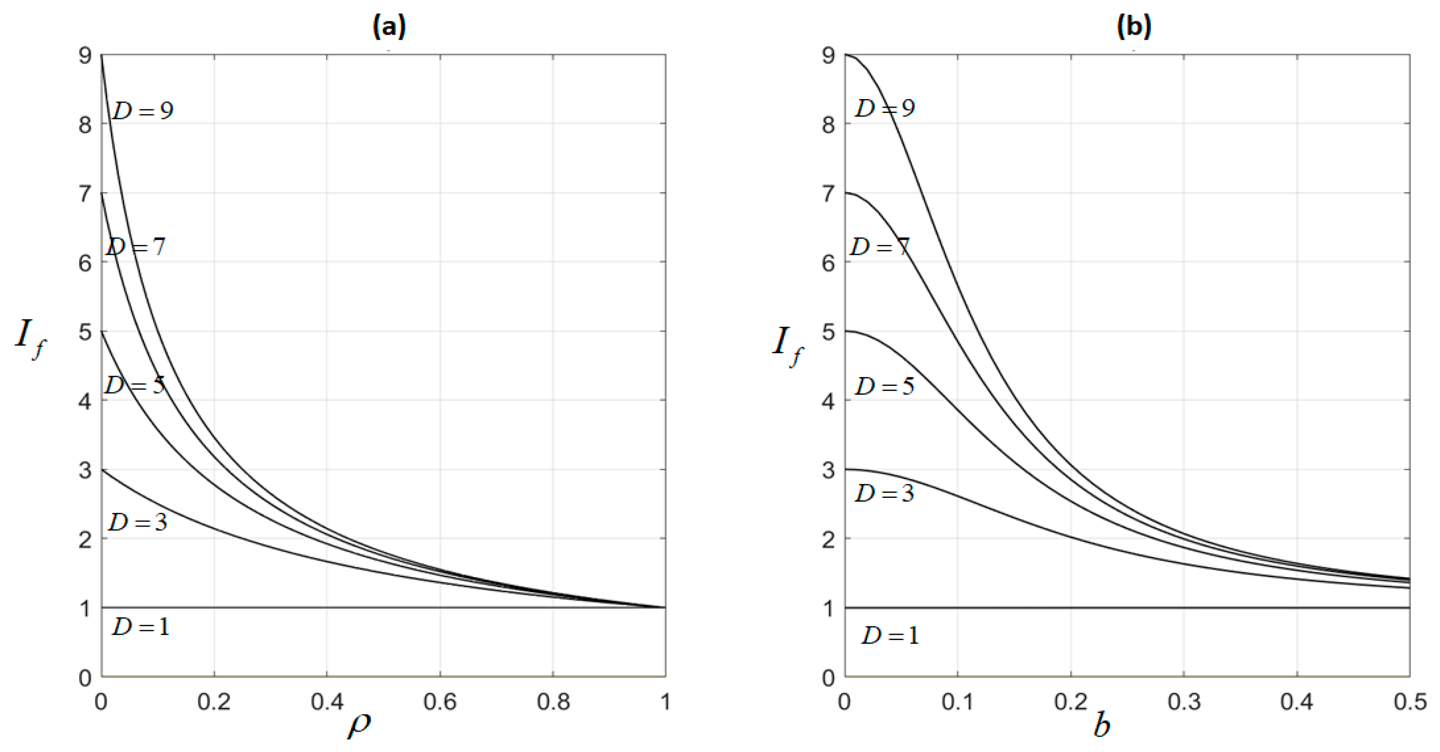
We showed that, in the EOC case, the parameters affecting the improvement factor, $I_f$, are the number of classifiers, $D$; the pairwise correlation, $\rho$; and the bias, $b$. This is illustrated in Figure 2. Thus, in Figure 2a, we show $I_f$ as a function of $\rho$ for different values of $D$; bias $b$ was assumed to be 0. We see that $I_f$ increases with $D$, but decreases with $\rho$ from a maximum value of $I_f=D$ for $\rho =0$ to a minimum value of $I_f=1$ for $\rho =1$. Similarly, in Figure 2b, we show $I_f$ as a function of $b$ for different values of $D$; correlation $\rho$ was assumed to be 0. Again, $I_f$ increases with $D$, but, as expected, decreases for an increasing bias.

Let us finally compute the optimum coefficient vector, $w$, corresponding to the EOCs.

$$\begin{array}{l}{w}_{LLMSE}={\displaystyle \frac{M_s^{-1}1}{1^T{M}_s^{-1}1}}={\displaystyle \frac{\left(1-\rho \right)\nu +D\left(\rho \nu +b^2\right)}{D}}{\displaystyle \frac{1}{\left(1-\rho \right)\nu }}\left(I-{\displaystyle \frac{\rho \nu +b^2}{\left(1-\rho \right)\nu +D\left(\rho \nu +b^2\right)}}11^T\right)1=\\ ={\displaystyle \frac{\left(1-\rho \right)\nu +D\left(\rho \nu +b^2\right)}{D}}{\displaystyle \frac{1}{\left(1-\rho \right)\nu }}\left(1-{\displaystyle \frac{\left(\rho \nu +b^2\right)D}{\left(1-\rho \right)\nu +D\left(\rho \nu +b^2\right)}}\right)1={\displaystyle \frac{1}{D}}{\displaystyle \frac{1}{\left(1-\rho \right)\nu }}\left(\left(1-\rho \right)\nu \right)1={\displaystyle \frac{1}{D}}1\end{array}.$$

(16)

Thus, as expected, the mean of the scores is the LLMSE solution in the case of EOCs, always achieving an improvement factor of $1\le I_f\le D$.

3.2. Fusion of Non-Equally Operated Classifiers (NEOCs)

Notice that, in the case of individual classifiers with disparate performances, it is reasonable to consider that the scores they provide are uncorrelated. This simplifies an analysis that would otherwise be intractable. Furthermore, as for the EOCs, we assume for simplicity that the covariance–bias model is the same for both classes; then:

$$C_s=C_{s/0}=C_{s/1}=\left(\begin{array}{ccc}{\nu }_1& 0& 0\\ 0& \ddots & 0\\ 0& 0& {\nu }_D\end{array}\right)={\Lambda }_s; b_s=b_{s/0}=b_{s/1}=\left[\begin{array}{c}{b}_1\\ ⋮\\ b_D\end{array}\right],$$

(17)

Let us use Miller’s lemma again to calculate the inverse of $M_s={\Lambda }_s+b_s{b}_s^T$:

$$M_s^{-1}={\left({\Lambda }_s+b_s{b}_s^T\right)}^{-1}={\Lambda }_s^{-1}-{\displaystyle \frac{1}{1+trace\left(b_s{b}_s^T{\Lambda }_s^{-1}\right)}}{\Lambda }_s^{-1}{b}_s{b}_s^T{\Lambda }_s^{-1}.$$

(18)

Then:

$$\begin{array}{l}MS{E}_f={\displaystyle \frac{1}{1^T{M}_s^{-1}1}}={\displaystyle \frac{1}{1^T\left({\Lambda }_s^{-1}-\frac{1}{1+trace\left(b_s{b}_s^T{\Lambda }_s^{-1}\right)}{\Lambda }_s^{-1}{b}_s{b}_s^T{\Lambda }_s^{-1}\right)1}}=\\ ={\displaystyle \frac{1}{{\displaystyle \sum _{d=1}^D\frac{1}{v_d}-\frac{1}{1+{\displaystyle \sum _{d=1}^D\frac{b_d^2}{v_d}}}{\left({\displaystyle \sum _{d=1}^D\frac{b_d}{v_d}}\right)}^2}}}\end{array}.$$

(19)

And, finally:

$$I_f={\displaystyle \frac{MS{E}_D}{MS{E}_f}}=\left(v_D+b_D^2\right)\left({\displaystyle \sum _{d=1}^D\frac{1}{v_d}-\frac{1}{1+{\displaystyle \sum _{d=1}^D\frac{b_d^2}{v_d}}}{\left({\displaystyle \sum _{d=1}^D\frac{b_d}{v_d}}\right)}^2}\right).$$

(20)

This is a complicated expression due to the arbitrary combinations of bias and variance in each individual classifier. However, we can impose some simplification to gain insights into the expected improvement. Thus, we may consider that all the individual scores have the same bias, $b_1=b_2=\dots =b_D=b$. Then, we can write:

$$\begin{array}{l}{I}_f={\displaystyle \frac{MS{E}_D}{MS{E}_f}}=\left(v_D+b^2\right)\left({\displaystyle \sum _{d=1}^D\frac{1}{v_d}-\frac{1}{1+b^2{\displaystyle \sum _{d=1}^D\frac{1}{v_d}}}{b}^2{\left({\displaystyle \sum _{d=1}^D\frac{1}{v_d}}\right)}^2}\right)=\left(v_D+b^2\right){\displaystyle \frac{{\displaystyle \sum _{d=1}^D\frac{1}{v_d}}}{1+b^2{\displaystyle \sum _{d=1}^D\frac{1}{v_d}}}}=\\ ={\displaystyle \frac{v_D{\displaystyle \sum _{d=1}^D\frac{v_D}{v_d}+b^2{\displaystyle \sum _{d=1}^D\frac{v_D}{v_d}}}}{v_D+b^2{\displaystyle \sum _{d=1}^D\frac{v_D}{v_d}}}}={\displaystyle \frac{C{v}_D+C{b}^2}{v_D+C{b}^2}}\end{array},$$

(21)

where, $C={\displaystyle \sum _{d=1}^D\frac{v_D}{v_d}}$. Considering that $0\le {\displaystyle \frac{v_D}{v_d}}\le 1d=1\dots D-1$, $1\le C\le D$. If $v_D\ll v_d ,d=1\dots D-1$, we have a very unbalanced scenario; then, $C=1\Rightarrow I_f=1$, i.e., if the best classifier is “much better” than the rest, little improvement can be expected from the fusion. In the opposite case, we have a totally balanced situation if $v_D=v_d=1,d=1\dots D-1$, and then $C=D$. Moreover, $I_f$ reaches its maximum ${\displaystyle \frac{D{v}_D+D{b}^2}{v_D+D{b}^2}}$, which consistently coincides with (15) (this is actually the EOC case with uncorrelated classifiers). In general, every classifier contributes ${\displaystyle \frac{v_D}{v_d}}$ to increase $I_f$. Let us define the unbalanced factor $U={\displaystyle \frac{D-C}{D-1}} D>1$ such that $0\le U\le 1$, being $U=0$ in the totally balanced case ($C=D$), and $U=1$ for the very unbalanced case ($C=1$).

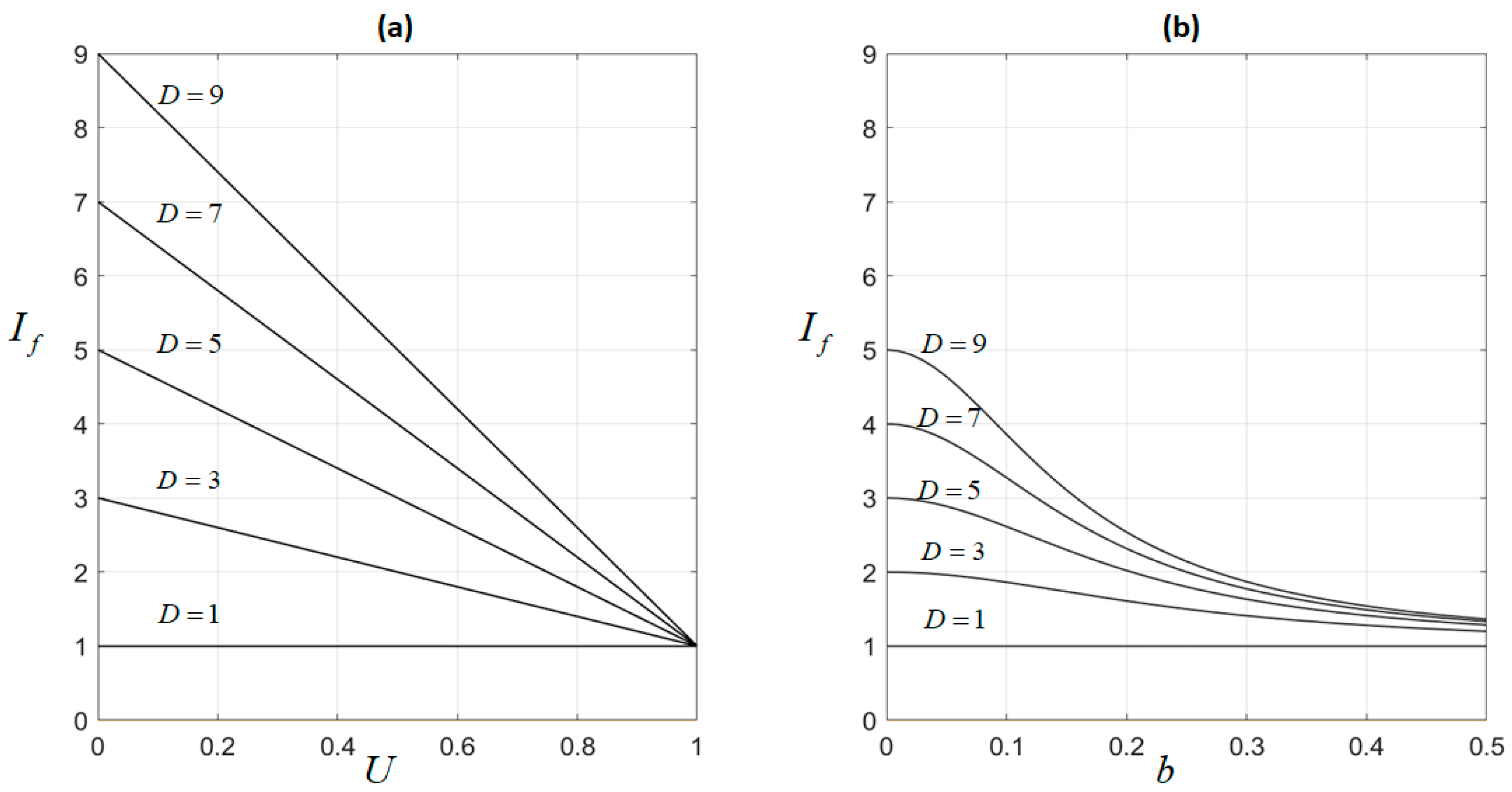
We showed that, in NEOCs, the parameters affecting the improvement factor, $I_f$, are the number of classifiers, $D$; the unbalance factor, $U$; and the bias, $b$. This is illustrated in Figure 3. Thus, in Figure 3a, we show $I_f$ as a function of $U$ for different values of $D$; bias was assumed to be 0. According to (21), this implies that $I_f=C=-U\left(D-1\right)+D$, explaining the decreasing straight line varying from a maximum value of $I_f=D$ for $U=0$ to a the minimum value of $I_f=1$ for $U=1$. Similarly, in Figure 3b, we show $I_f$ as a function of $b$ for different values of $D$; the unbalance factor $U$ was assumed to be $U=0.5$. Again, $I_f$ decreases for the increasing bias. Moreover, notice that Figure 2b and Figure 3b show similar curves, but in the first case, $U=0$ (all classifiers show an equal performance), while $U=0.5$ is assumed in the second case; then, $I_f$ suffers a certain degradation, reaching the maximum value of $I_f=C=-0.5\left(D-1\right)+D=0.5\left(D+1\right)$ for $b=0$.

Let us finally compute the optimum coefficient vector, $w$, corresponding to the NEOCs. Thus:

$$\begin{array}{l}{w}_{LLMSE}={\displaystyle \frac{M_s^{-1}1}{1^T{M}_s^{-1}1}}=MS{E}_f{M}_s^{-1}1=MS{E}_f\left({\Lambda }_s^{-1}-{\displaystyle \frac{1}{1+trace\left(b_s{b}_s^T{\Lambda }_s^{-1}\right)}}{\Lambda }_s^{-1}{b}_s{b}_s^T{\Lambda }_s^{-1}\right)1=\\ =MS{E}_f\left(I-{\displaystyle \frac{1}{1+trace\left(b_s{b}_s^T{\Lambda }_s^{-1}\right)}}{\Lambda }_s^{-1}{b}_s{b}_s^T\right){\Lambda }_s^{-1}1\end{array}.$$

(22)

We see that the optimum linear combiner is the vector ${\Lambda }_s^{-1}1={\left[{\displaystyle \frac{1}{{\nu }_1}}\dots {\displaystyle \frac{1}{{\nu }_D}}\right]}^T$, which gives more relevance to the classifiers having a smaller variance, minus the linear transformation of this vector, which depends on the bias contributions. Actually, $b_s=0\Rightarrow w_{LLMSE}={\left[{\displaystyle \frac{1}{{\nu }_1}}\dots {\displaystyle \frac{1}{{\nu }_D}}\right]}^T$.

4. From Mean Square Error to Probability of Error

Given a score, $s$, we have to decide between $c_0$ and $c_1$. Interpreting $s$ as the posterior probability of $c_1$, we implement the MAP test:

$$s\begin{array}{c}\stackrel{c_1}{>}\\ \underset{c_0}{<}\end{array}{\displaystyle \frac{1}{2}}.$$

(23)

Then, the performance of the classifier can be evaluated by the probability of error, $P_{\epsilon }$. Obviously, the lower the $MSE$, the lower $P_{\epsilon }$ should be. However, this is not demonstrable in a general case, as both the $MSE$ and $P_{\epsilon }$ are quite different integrals of the class-conditional probability density functions (pdfs), namely:

$$\begin{array}{l}MSE=E\left[{\left(u-s\right)}^2\right]=P_0\cdot E\left[{\left(u-s\right)}^2/c_0\right]+P_1\cdot E\left[{\left(u-s\right)}^2/c_1\right]=\\ =P_0{\displaystyle {\int }_0^1{\left(0-s\right)}^2}p\left(s/c_0\right)ds+P_1{\displaystyle {\int }_0^1{\left(1-s\right)}^2}p\left(s/c_1\right)ds\\ P_{\epsilon }=P_0\cdot {\displaystyle {\int }_{\frac{1}{2}}^{1}p\left(s/c_0\right)ds}+P_1\cdot {\displaystyle {\int }_0^{\frac{1}{2}}p\left(s/c_1\right)ds}\end{array}.$$

(24)

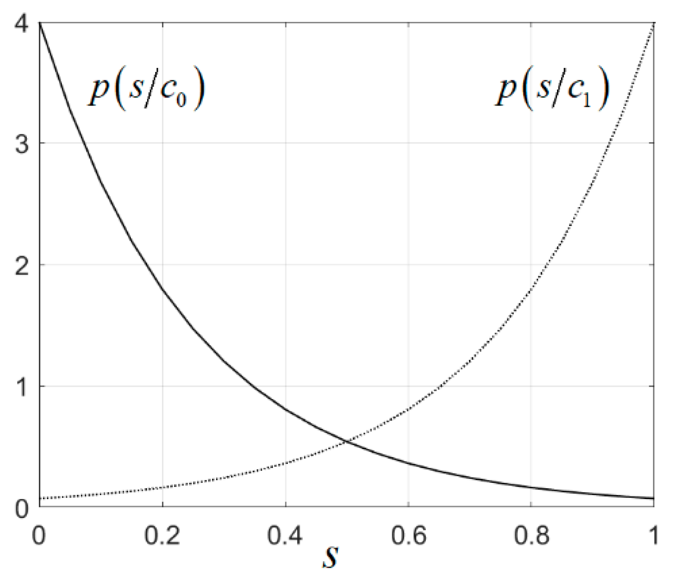
For this reason, we now assume a simple but representative model of the conditional pdfs. Let us consider that $p\left(s/c_1\right)$ and $p\left(s/c_0\right)$ are exponential pdfs in the interval $\left(0,1\right)$, i.e.,

$$p\left(s/c_0\right)={\lambda }_0{e}^{-{\lambda }_{0}s}u\left(s\right)p\left(s/c_1\right)={\lambda }_1{e}^{-{\lambda }_1\left(1-s\right)}u\left(1-s\right).$$

(25)

where $u\left(s\right)$ is the unit step function. In (25), we assumed that ${\lambda }_0$ and ${\lambda }_1$ are large enough so that ${\lambda }_0{e}^{-{\lambda }_{0}s}\simeq 0s>1{\lambda }_1{e}^{-{\lambda }_1\left(1-s\right)}\simeq 0s<0$, and so the exponentials are appropriate pdfs for scores. We show in Figure 4 two exponential class-conditional pdfs for ${\lambda }_0={\lambda }_1=4$.

We can express $P_{\epsilon }$ is (24) as the combination of the probability of false-positives, $P_{\epsilon I}$ (type I error), and the probability of false negatives, $P_{\epsilon II}$ (type II error), and considering (23) and the exponential models (25), we have:

$$\begin{array}{l}{P}_{\epsilon }=P_0\cdot P_{{\epsilon }_I}+P_1\cdot P_{{\epsilon }_{II}}\\ P_{{\epsilon }_I}={\displaystyle {\int }_{\frac{1}{2}}^{1}p\left(s/c_0\right)ds}=P_0\cdot {\displaystyle {\int }_{\frac{1}{2}}^1{\lambda }_0{e}^{-{\lambda }_{0}s}ds}\simeq P_0\cdot {\displaystyle {\int }_{\frac{1}{2}}^{\infty }{\lambda }_0{e}^{-{\lambda }_{0}s}ds}=e^{-{\displaystyle \frac{{\lambda }_0}{2}}}\\ P_{{\epsilon }_{II}}={\displaystyle {\int }_0^{\frac{1}{2}}p\left(s/c_1\right)ds}={\displaystyle {\int }_0^{\frac{1}{2}}{\lambda }_1{e}^{-{\lambda }_1\left(1-s\right)}ds=}{\displaystyle {\int }_{\frac{1}{2}}^1{\lambda }_1{e}^{-{\lambda }_{1}s\prime }ds\prime }\simeq {\displaystyle {\int }_{\frac{1}{2}}^{\infty }{\lambda }_1{e}^{-{\lambda }_{1}s\prime }ds\prime }=e^{-{\displaystyle \frac{{\lambda }_1}{2}}}\end{array}.$$

(26)

In general, as we did in (2) for the fused score, we can express the MSE as the combination of the MSEs conditional to every possible value of the random variable, $u$.

$$\begin{array}{l}MSE=E\left[{\left(u-s\right)}^2\right]=P_0\cdot MS{E}_I+P_1\cdot MS{E}_{II}\\ MS{E}_I={\left(0-E\left[s/c_0\right]\right)}^2+\mathrm{var}\left[s/c_0\right]={\left({\displaystyle \frac{1}{{\lambda }_0}}\right)}^2+{\displaystyle \frac{1}{{\lambda }_0^2}}={\displaystyle \frac{2}{{\lambda }_0^2}}\\ MS{E}_{II}={\left(1-E\left[s/c_1\right]\right)}^2+\mathrm{var}\left[s/c_1\right]={\left(1-\left(1-{\displaystyle \frac{1}{{\lambda }_1}}\right)\right)}^2+{\displaystyle \frac{1}{{\lambda }_1^2}}={\displaystyle \frac{2}{{\lambda }_1^2}}\end{array}.$$

(27)

Solving for ${\lambda }_0$ and ${\lambda }_1$ in (27) and substituting in (26), we arrive at:

$$P_{\epsilon }=P_0\cdot e^{-{\displaystyle \frac{1}{\sqrt{2MS{E}_I}}}}+P_1\cdot e^{-{\displaystyle \frac{1}{\sqrt{2MS{E}_{II}}}}}.$$

(28)

Thus, in (28), we see the definite impact that the minimization of the MSE has on the minimization of the probability of error. Hence, it is of great interest to relate the improvement factor previously defined with the expected improvement of $P_{\epsilon f}$ with respect to $P_{\epsilon D}$. This is straigthforward in the case that ${\lambda }_0={\lambda }_1\Rightarrow MS{E}_I=MS{E}_{II}$:

$$P_{\epsilon f}=e^{-{\displaystyle \frac{1}{\sqrt{2MS{E}_f}}}}=e^{-{\displaystyle \frac{\sqrt{I_f}}{\sqrt{2MS{E}_D}}}}={\left(P_{\epsilon D}\right)}^{\sqrt{I_f}},$$

(29)

But, in general, we need to define a separate improvement factor for every type of error:

$I_{fI}={\displaystyle \frac{MS{E}_{DI}}{MS{E}_{fI}}},I_{fII}={\displaystyle \frac{MS{E}_{DII}}{MS{E}_{fII}}}$, so that

$$P_{\epsilon f}=P_0\cdot P_{\epsilon DI}{}^{\sqrt{I_{fI}}}+P_1\cdot P_{\epsilon DII}{}^{\sqrt{I_{fII}}}.$$

(30)

Let us show some illustrative examples for the above. We consider, for simplicity, the case ${\lambda }_0={\lambda }_1$. Let us define the theoretical accuracy $A=1-P_{\epsilon }$. Using (29), we represent in Figure 5a the post-fusion accuracy, $A_f$, as a function of the accuracy, $A_D$, of the best classifier for different values of $I_f$. The significant increase in accuracy with the increase in $I_f$ is notable. Thus, for example, a value of $A_D=0.70$ increases to $A_f=0.87$ for $I_f=3$. From the previous analysis, we know that 3 uncorrelated and unbiased classifiers would be enough to provide such an improvement factor. Furthermore, we represent in Figure 5b the accuracy, $A_f$, as a function of $I_f$ for different values of $A_D$. Once again, the significant accuracy improvement that can be achieved with improvement factors that are not excessively high is notable. This is especially true for weak classifiers that provide relatively low accuracy.

5. Real Data Experiments

In this section, we consider some experiments with real data. This involves the automatic classification of sleep stages based on the information provided by different biosignals (polysomnograms). This classification is usually performed manually by a medical expert, resulting in a slow and tedious procedure. In particular, we consider the detection of very-short periods of wakefulness [29,30] (also called arousals) as their frequency is related to the presence of apnea and epilepsy. The objective is by no means to present the most-precise method for solving this complex problem, among the myriad of options and variants available. Rather, it is to verify in a real-life context how the fusion of several classifiers achieves results consistent with the theory outlined above. The data were obtained from the public database Physionet [31]. Ten patients were considered. Every patient was monitored during sleep, thus obtaining the corresponding polysomnogram. In this experiment, we considered the electroencephalograms (EEGs). Then, 8 EEG features were obtained in non-overlapping intervals of 30 sec (epochs) from every EEG recording. The number of epochs varied for every patient, ranging from 749 (6 h and 14 min) to 925 (7 h and 42 min). The 8 features were: Powers in the frequency bands delta (0–4 Hz), theta (5–7 Hz), alpha (8–12 Hz), sigma (13–15 Hz), and beta (16–30 Hz), and 3 Hjorth parameters: activity, mobility, and complexity. These features are routinely used in the analysis of EEG signals [32,33].

As we were interested in the detection of arousals, a two-class problem was considered, where class 1 corresponded to arousal and class 0 corresponded to any of the other possible sleep stage. This is in concordance with the two-class scenario assumed in the previous theoretical analysis.

Five classifiers were considered: Gaussian Bayes, Gaussian Naïve Bayes, Nearest Mean, Linear Discriminant, and Logistic Regression.

Table 1. Score computation method and required training.

Method	Score	Training
Gaussian Bayes	$s_d={\displaystyle \frac{e^{-\frac{1}{2}\left({\left(x-{\mu }_1\right)}^T{C}_1^{-1}\left(x-{\mu }_1\right)\right)}}{e^{-\frac{1}{2}\left({\left(x-{\mu }_1\right)}^T{C}_1^{-1}\left(x-{\mu }_1\right)\right)}+e^{-\frac{1}{2}\left({\left(x-{\mu }_0\right)}^T{C}_0^{-1}\left(x-{\mu }_0\right)\right)}}}$	${\widehat{\mu }}_1,{\widehat{\mu }}_0,{\widehat{C}}_1,{\widehat{C}}_0$ (ML sample estimates)
Gaussian Naïve Bayes	$s_d={\displaystyle \frac{e^{-\frac{1}{2{\sigma }_1^2}\left({\left(x-{\mu }_1\right)}^T\left(x-{\mu }_1\right)\right)}}{e^{-\frac{1}{2{\sigma }_1^2}\left({\left(x-{\mu }_1\right)}^T\left(x-{\mu }_1\right)\right)}+e^{-\frac{1}{2{\sigma }_0^2}\left({\left(x-{\mu }_0\right)}^T\left(x-{\mu }_0\right)\right)}}}$	${\widehat{\mu }}_1,{\widehat{\mu }}_0,{\widehat{\sigma }}_1^2,{\widehat{\sigma }}_0^2$ (ML sample estimates)
Nearest Mean	$s_d={\displaystyle \frac{e^{-\frac{1}{2}{‖x-{\mu }_1‖}^2}}{e^{-\frac{1}{2}{‖x-{\mu }_1‖}^2}+e^{-\frac{1}{2}{‖x-{\mu }_0‖}^2}}}$	${\widehat{\mu }}_1,{\widehat{\mu }}_0$ (ML sample estimates)
Linear Discriminant	$s_d={\displaystyle \frac{w_1^{T}x}{w_1^{T}x+w_0^{T}x}}$	${\widehat{w}}_1,{\widehat{w}}_0$ (Respective solutions to two overdetermined systems of equations)
Logistic Regression	$s_d={\displaystyle \frac{1}{1+e^{-w^{T}x}}}$	$\widehat{w}$ (Solutions to one overdetermined system of equations)

indicates the equations corresponding to the score computation in every method, as well as the estimated parameters during training.

The classifiers were separately trained for every patient using the first half of the respective EEG recordings. Then, the second half was used for testing. The scores of all patients were grouped by classes. Thus, a total number of 6706 scores of class 0 and 1708 of class 1 were generated by every classifier. Despite this imbalanced scenario, we assumed that $P_0=P_1=0.5$ in all the experiments, in order to not harm the detection of arousals, which was a priority in this particular context.

Table 2. Estimates of the score statistics and accuracy of the classifiers. Correlated case.

	${\widehat{b}}_{d/0}$	${\widehat{b}}_{d/1}$	${\widehat{\nu }}_{d/0}$	${\widehat{\nu }}_{d/1}$	$M\widehat{S}{E}_d$	$\widehat{A}c{c}_d$
Nearest-mean	0.1047	0.2562	0.0539	0.1120	0.1213	83.29%
Linear Discr.	0.1175	0.3901	0.0221	0.0618	0.1250	82.99%
Gauss. Bayes	0.0670	0.2916	0.0469	0.1691	0.1528	82.55%
Naive Bayes	0.0686	0.3011	0.0492	0.1826	0.1636	82.08%
Logistic Regr.	0.0401	0.3586	0.0371	0.2242	0.1957	79.99%
	${\widehat{b}}_{f/0}$	${\widehat{b}}_{f/1}$	${\widehat{\nu }}_{f/0}$	${\widehat{\nu }}_{f/1}$	$M\widehat{S}{E}_f$	$\widehat{A}c{c}_f$
FUSION	0.1264	0.3032	0.0408	0.0670	0.1078	84.23%

shows the samples’ estimates of the score bias and variance for every class and every method, according to the definitions of (2) and (3). We can see that class 1 exhibits a significantly higher bias and variance than class 0 in all the five methods. The corresponding MSE and the accuracy are also indicated in Table 2 and used to rank the methods from “the best” (top) to the “worst” (bottom). The last row of Table 2 shows the statistics corresponding to the scores of the optimal linear combiner (6). Matrix $M_s$ was estimated from the scores of the training set, using sample estimates in (5) for the covariance and bias matrices. Notice that, as expected, the bias of the fused scores does not show a reduction with respect to the bias of the individual classifiers. However, the variance is reduced, this effect being the main reason from the MSE decrease and corresponding accuracy increase achieved by the fusion of classifiers. Certainly, the improvement is modest due in part to the high correlation among the scores of the 5 individual classifiers, as indicated by the correlation coefficient matrices included at the bottom of Table 2. Furthermore, significant bias, especially in class 1, is also an issue for obtaining greater improvements. In any case, these real data results are in concordance with the expectation of the theoretical analysis.

$${\widehat{\rho }}_0=\left[\begin{array}{l}1.000.870.760.840.64\\ 0.871.000.680.700.70\\ 0.760.681.000.890.52\\ 0.840.700.891.000.56\\ 0.64 0.700.520.561.00\end{array}\right]{\widehat{\rho }}_1=\left[\begin{array}{l}1.000.770.780.850.70\\ 0.771.000.680.670.84\\ 0.780.681.000.890.61\\ 0.850.670.891.000.61\\ 0.700.840.610.611.00\end{array}\right]$$

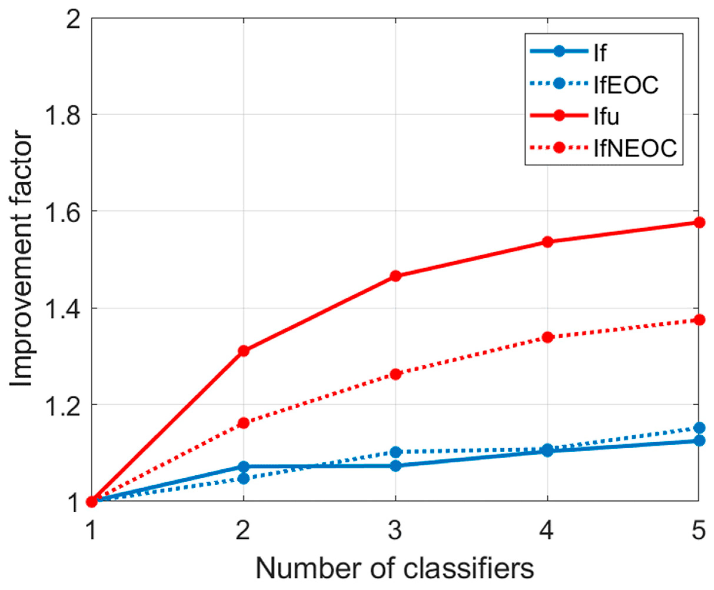
With the intention of reinforcing this perception, we show in Figure 6 (solid blue) the variation in the improvement factor with the number of fused classifiers. Starting from $D=1$ with the Nearest Mean, which is the best individual classifier according to Table 2, we progressively incorporate a new classifier following the order of Table 2. We can see that $I_f$ increases with $D$ as predicted by the theory, but shifts rather slowly due to the high correlation and large bias. We also represent in Figure 6 (blue dot) the improvement factor of the EOC case computed from (14) for every $D$, where $\nu ,\rho$, and $b^2$ are estimated as:

$$\widehat{\nu }={\displaystyle \frac{1}{D}}{\displaystyle \sum _{d=1}^D{\widehat{v}}_d};\widehat{\rho }={\displaystyle \frac{1}{D}}\sqrt{{‖\widehat{\rho }‖}_F^2-D};{\widehat{b}}^2={\displaystyle \frac{1}{D}}{‖{\widehat{b}}_s{\widehat{b}}_s^T‖}_F$$

(31)

where ${\widehat{v}}_d={\displaystyle \frac{1}{2}}\left({\widehat{\nu }}_{d/0}+{\widehat{\nu }}_{d/1}\right)$, $\widehat{\rho }={\displaystyle \frac{1}{2}}\left({\widehat{\rho }}_0+{\widehat{\rho }}_1\right)$, and ${\widehat{b}}_s={\displaystyle \frac{1}{2}}\left({\widehat{b}}_{s/0}+{\widehat{b}}_{s/1}\right)$ are obtained from the results of Table 2. Thus, the Frobenius norms, ${‖\cdot ‖}_F$, of the correlation coefficient and the bias (constant entries) matrices of the EOC model, respectively, equate the Frobenios norms of the corresponding (non-constant entries) real-data matrices. In essence, we define an EOC model that “resembles” as much as possible the actual real-data model. Figure 6 suggests that the EOC model, in spite of its simplicity, can provide a reasonably approximation of the actual $I_f$ value.

We conducted another experiment, where the scores of each classifier are much more uncorrelated than in the previous experiment. To simulate high decorrelation, the inputs to the different classifiers in the interval under test are randomly selected (sampling with replacement) from all the available feature vectors of the training set that belong to the true class of that interval. In this way, the inputs to the different classifiers in each test interval belong to the same class, but are generally different, producing a high level of decorrelation between the scores obtained from them. This procedure serves to simulate decorrelation, but is not practical since the class being tested must be known in advance. In a practical situation, decorrelation must be obtained through appropriate training, for example, bagging-type techniques [34], in which the same classifier is trained with different subsets of instances obtained from an original set. The hard decisions of the differently trained classifiers are combined to obtain a final decision. More generally, in classifier fusion, each classifier can be trained on different subsets of instances to induce some level of score uncorrelation. Another scenario where the scores can be uncorrelated is in late-multimodal fusion [9], where the input of each individual classifier corresponds to a different modality.

We show in

Table 3. Estimates of the score statistics and accuracy of the classifiers. Uncorrelated case.

	${\widehat{b}}_{d/0}$	${\widehat{b}}_{d/1}$	${\widehat{\nu }}_{d/0}$	${\widehat{\nu }}_{d/1}$	$M\widehat{S}{E}_d$	$\widehat{A}c{c}_d$
Nearest-mean	0.1034	0.2656	0.0533	0.1146	0.1246	82.93%
Linear	0.1180	0.3905	0.0223	0.0638	0.1263	82.80%
Bayes	0.0680	0.2859	0.0476	0.1672	0.1506	82.65%
Naive Bayes	0.0649	0.2952	0.0458	0.1788	0.1580	81.72%
Logistic	0.0398	0.3525	0.0370	0.2236	0.1932	80.34%
	${\widehat{b}}_{f/0}$	${\widehat{b}}_{f/1}$	${\widehat{\nu }}_{f/0}$	${\widehat{\nu }}_{f/1}$	$M\widehat{S}{E}_f$	$\widehat{A}c{c}_f$
FUSION	0.0845	0.3081	0.0110	0.0449	0.0790	89.60%

the same type of information shown in Table 2. Notice that the statistics of the individual classifiers are quite similar to those in Table 2, however the post-fusion MSE has been significantly reduced (mainly because of the variance reduction), and the accuracy has improved by 7% with respect to the best classifier. Notice the low level of correlation (especially in class 0), as indicated by the correlation coefficient matrices included at the bottom of Table 3.

$${\widehat{\rho }}_0=\left[\begin{array}{l}1.000.080.010.030.04\\ 0.081.000.010.010.07\\ 0.010.011.000.030.02\\ 0.030.010.031.000.00\\ 0.04 0.070.020.001.00\end{array}\right]{\widehat{\rho }}_1=\left[\begin{array}{l}1.000.120.160.170.06\\ 0.121.000.120.150.13\\ 0.160.121.000.270.10\\ 0.170.150.271.000.08\\ 0.060.130.100.081.00\end{array}\right]$$

The comparative impact of uncorrelation can be better appreciated in Figure 6, where we show (solid red) the variation in the improvement factor in the case of uncorrelation, $I_{fu}$, with the number of fused classifiers. Notice the significant increase in the improvement factor with respect to the correlated case ($I_f$). We also represent in Figure 6 (red dot) the improvement factor, $I_{fNEOC}$, of the NEOC case computed from (21) for every $D$, where $\widehat{C}={\displaystyle \sum _{d=1}^D\frac{{\widehat{v}}_D}{{\widehat{v}}_d}}$; ${\widehat{v}}_d d=1\dots D$ as well as $b^2$ are computed as in (31). $I_{fNEOC}$ shows a similar evolution to $I_{fu}$, but with some underestimation. Notice that ${\widehat{v}}_D$ corresponds to the actual variance of the Linear classifier, which is the minimum variance among all the 5 classifiers, as deduced from Table 2. However, the $MS{E}_D$ value considered to compute $I_{fu}$ is that corresponding to the Nearest Mean, which is the minimum MSE among all the 5 classifiers, as deduced from Table 2. This probably means facing an additional problem to achieve a good fit of the NEOC model to the actual model, because in the NEOC model, the bias is assumed to be the same for all classifiers, and then both ${\widehat{v}}_D$ and $MS{E}_D$ correspond to the same classifier. In any case, notice that $I_{fNEOC}$ is still far from 5, the maximum achievable value if all the classifiers are unbaised. This is evidence of the significant limitation imposed by bias in the fusion of classifiers. Another limitation to achieving maximum improvement in the NEOC model was the unbalance factor $U={\displaystyle \frac{D-C}{D-1}}$. In our case, $U$ has a value between 0.5 and 0.6 for all values of $D$, which is between the perfectly balanced case ($U=0$) and the totally unbalanced case ($U=1$).

Finally, we show in Figure 7 the variation in estimated accuracy with the number of classifiers for the correlated (blue solid) and the uncorrelated (red solid) cases. Similar to $I_f$, the accuracy slowly increases with $D$ in the correlated case. And, similar to $I_{fu}$, the increase is more significant in the uncorrelated case. We also show in Figure 7 (blue dot and red dot) the theoretical accuracies predicted by Equation (30), assuming $P_0=P_1=0.5$, namely:

$$\begin{array}{l}{A}_{ft}=1-P_{\epsilon ft}=1-0.5\cdot \left({P_{\epsilon DI}}^{\sqrt{I_{fI}}}+{P_{\epsilon DII}}^{\sqrt{I_{fII}}}\right)\\ A_{fut}=1-P_{\epsilon fut}=1-0.5\cdot \left({P_{\epsilon DuI}}^{\sqrt{I_{fuI}}}+{P_{\epsilon DuII}}^{\sqrt{I_{fuII}}}\right)\end{array},$$

(32)

where $P_{\epsilon DI}$ and $P_{\epsilon DII}$ are the respective actual probabilities of errors type I and type II of the best classifiers in the correlated case. And similarly, with respect to $P_{\epsilon DuI}$ and $P_{\epsilon DuII}$.

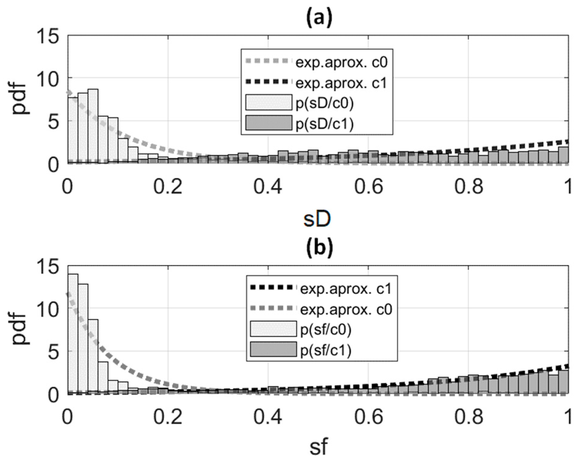
We can see the good fitting between the theoretical prediction and the actually computed accuracies. This suggests that the exponential model assumed to deduce (30) is appropriate for the fused scores and for the scores of the best classifier. This can be corroborated if we look at Figure 8, which shows histograms normalized to represent the non-parametric estimates of pdfs. We show in Figure 8a the histograms corresponding to the pdf estimates of the best classifiers $\widehat{p}\left(s_D/c_0\right)$ (left) and $\widehat{p}\left(s_D/c_1\right)$ (right). Furthermore, we show in Figure 8b the histograms corresponding to the pdf estimates of the fused scores $\widehat{p}\left(s_f/c_0\right)$ (left) and $\widehat{p}\left(s_f/c_1\right)$ (right). The exponential approximations are superimposed. Every exponential approximation was made from the ML estimates of the corresponding parameter, i.e., $\widehat{\lambda }={\displaystyle \frac{1}{\widehat{E}\left[s\right]}}$, where $\widehat{E}\left[s\right]$ is the sample mean of the scores.

In order to gain greater confidence, we performed some additional experiments. Firstly, we take into account the imbalance scenario. Thus, we conducted various experiments using either the oversampling of the least-abundant class or undersampling of the most-abundant class. For oversampling, we used the generative network-based GANSO [35,36], which demonstrated its superiority over the classic SMOTE method. To subsample, we simply removed instances of the most-abundant class until we reached the training size of the least-abundant one. The results do not differ significantly from those shown in Table 2 and Table 3. On the other hand, with the intention of gaining statistical consistency, we repeated the previous experiments 100 times, obtaining the mean values and standard deviations of all the parameters shown in Table 2 and Table 3. In each repetition, a different partition of the training and testing sets is considered (always at 50 percent). The mean values are similar to the data in Table 2 and Table 3. The standard deviations never exceed 2% of the mean values. We also performed a significance test on the accuracies obtained by the fusion, characterizing the distribution of the null hypothesis with the 100 accuracy values obtained with the best of the individual classifiers. In all cases, the p-value is less than 0.05, so the null hypothesis is rejected, and we can consider that the accuracy values from the fusion are statistically significant. In conclusion, the results in Table 2 and Table 3 are sufficiently illustrative for the purpose of reinforcing the theoretical analysis (the focus of this research), with some experimental verification.

6. Discussion and Conclusions

The main objective of this work is to contribute, through mathematical analysis, to a better understanding of the soft fusion of classifiers. To perform this analysis, a combiner is proposed that provides the LLMSE estimator of the binary random variable associated with the two-class problem. The LLMSE thus obtained is expressed in terms of the properties of the individual classifiers, particularly their MSEs. All this leads to the definition of an improvement factor, which is the ratio of the MSE corresponding to the best classifier (the one with the minimum MSE) to the MSE provided by the fused score. Two simplified, yet relevant, models (EOC and NEOC) are considered to determine the key parameters affecting the expected improvement due to fusion. All in all, we concluded that those key parameters are the number of individual classifiers, the pairwise correlation among the individual scores, the bias, and the unbalance among the individual variances. In summary, we can say that it is interesting to fuse the largest number of classifiers, which preferably provide scores that are uncorrelated, unbiased, and with similar variances.

Ultimately, the classifier probability of error (or the accuracy) is the most important figure of merit. Therefore, we related the improvement in MSE to the expected accuracy improvement. To do so, we considered exponential models for the class-conditional pdfs. Although these are specific models, a clear connection between the MSE of the class estimation and the classifier performance was demonstrated.

The real data experiments showed consistency with the theoretical analysis, although the actual score models were different from the assumed in both EOC and NEOC models. Regarding accuracy, we verified the good fitting between the theoretical predictions and the actual data. This suggests that the score pdf exponential models are appropriate in this case.

Both the theoretical analysis and the experimental results encourage expanding this work in several respects. First, more general models than EOC and NEOC could better fit different real-world data scenarios. Second, it would be of great interest to seek methods capable of providing unbiased and uncorrelated scores. Specifically, the severe limitation on improvement imposed by bias suggests the merit of further investigation into this problem. The extension of the analysis to the multiclass problem and to unsupervised or semi-supervised scenarios [37,38] will be of undoubted interest. Additionally, other non-Bayesian fusion approaches, such as those based on the Dempster–Shafer theory, should be explored [39].