Article

Short-Term Power Load Prediction of VMD-LSTM Based on ISSA Optimization

1
School of Electrical and Electronic Engineering, Hubei University of Technology, Wuhan 430068, China
2
Xiangyang Industrial Institute, Hubei University of Technology, Xiangyang 210023, China
*
Author to whom correspondence should be addressed.
Appl. Sci. 2025, 15(9), 5037; https://doi.org/10.3390/app15095037
Submission received: 27 March 2025 / Revised: 27 April 2025 / Accepted: 28 April 2025 / Published: 1 May 2025

Abstract

:
Accurate short-term power load forecasting (STPLF) is critical for balancing electricity supply–demand and ensuring grid reliability. To address the challenges of fluctuating power loads and inaccurate predictions by conventional methods, this paper presents a novel hybrid framework combining Variational Mode Decomposition (VMD), Long Short-Term Memory (LSTM), and the Improved Sparrow Search Algorithm (ISSA). First, the power load series is decomposed into intrinsic mode functions (IMFs) via VMD, where the optimal decomposition order K is determined using permutation entropy (PE). Next, the decomposed IMFs and meteorological covariates are reconstructed into feature vectors, which are then input into the LSTM network for component-wise forecasting, and, finally, the prediction results of each component are reconstructed to obtain the final power load prediction result. The Improved Sparrow Search Algorithm (ISSA), which integrates piecewise chaotic mapping into population initialization to augment the global exploration capability, is employed to fine-tune LSTM hyperparameters, thereby enhancing the prediction precision. Finally, two case studies are conducted using Australian regional load data and Detu’an City historical load records. The experimental results indicate that the proposed model achieves reductions of 73.03% and 82.97% compared with the VMD-LSTM baseline, validating its superior predictive accuracy and cross-domain generalization capability.

1. Introduction

Electricity, as a foundational public utility underpinning national socioeconomic development, plays a critical role in sustaining industrial production, urban infrastructure, and the residential quality of life. As living standards rise, the electricity demand not only increases in quantity but also evolves toward more stringent requirements for power quality, including reliability, stability, and sustainability. The stochastic nature and time-varying volatility of power load profiles pose fundamental challenges to forecasting accuracy, particularly for short-term predictions. Therefore, rational power load planning and stable power system operations are critical for achieving smart grid objectives and enabling efficient energy management [1].
Current power load forecasting methods can be categorized into two primary groups: time-series statistical models and machine learning-based artificial intelligence techniques. Statistical load forecasting techniques encompass classical methods such as exponential smoothing [2], multiple linear regression [3], and autoregressive moving average models [4]. Classical statistical methods offer parsimonious theoretical foundations and a high computational efficiency, demonstrating a superior performance in linear problem domains. However, a fundamental drawback of classical statistical approaches lies in their linearity assumptions, which result in an inadequate nonlinear fitting and deteriorated prediction performance when applied to power loads characterized by nonlinear dynamics and high volatility. The machine learning algorithm has been widely used in the field of power load forecasting with its strong adaptive ability and excellent ability to process complex data. In particular, deep learning methods, which have flourished in recent years, have been favored by a wide range of scholars. Popular deep learning architectures for load forecasting include convolutional neural networks (CNNs) and recurrent neural networks (RNNs) [5] and so on. However, RNNs suffer from gradient vanishing or explosion issues in long-sequence modeling, prompting the development of Long Short-Term Memory (LSTM) [6,7,8] and the gated recurrent unit (GRU) [9,10,11]. These architectures mitigate gradient problems through gated mechanisms, demonstrating a superior performance in capturing long-term temporal dependencies. To further enhance feature extraction, some scholars have introduced a bidirectional LSTM (BiLSTM) [12,13] and bidirectional GRU (BiGRU) [14], leveraging forward–backward contextual information to improve trend capture. While bidirectional architectures enhance prediction accuracy, they concurrently increase computational complexity, creating a trade-off between performance and efficiency.
As the power load presents nonlinear and fluctuating characteristics, raw data inherently contain complex features that are challenging for single models to capture. To address this, a number of researchers have adopted some decomposition techniques, commonly including wavelet decomposition [15] and model decomposition [16,17,18,19], etc. These methods decompose load sequences into intrinsic mode components, effectively mitigating non-stationarity and reducing the adverse impact of random volatility on forecasting accuracy [20], and the experimental results show that these methods improve the prediction accuracy.
The literature [21] proposes a forecasting method based on EMD-BiLSTM, which firstly uses EMD to decompose the original power load data; then the decomposed data of different signals and weather features are reconstructed as input data. Then it uses BiLSTM to make a prediction, and finally superimposes the prediction results to obtain the final load. Notably, this model achieves an E M A P E of 0.28% and an R ² of 0.84 in empirical validation. Although the authors considered other feature factors, including weather, EMD suffers from computational inefficiency and is prone to modal aliasing. The literature [22] used EEMD to decompose the power load data into multiple Intrinsic Mode Functions (IMFs) with distinct frequency characteristics. These IMFs were classified into high-frequency and low-frequency components through a systematic zero-crossing rate analysis. Specifically, high-frequency components were modeled using a GRU neural network, while low-frequency components were forecasted via MLR. The hierarchical reconstruction of component-specific predictions was thereafter implemented to generate the final load forecasting results. The final load forecasting results show that most prediction points fall close to the true values without significant single-point errors, with an E M A P E of 4.86%. This indicates the method’s effectiveness in enhancing the prediction stability through the frequency-domain decomposition and adaptive modeling of different components. However, while this model mitigates mode mixing in conventional EMD through controlled noise injection, it may also lead to residual noise. The literature [23] proposes the use of CEEMD to decompose the non-stationary wind power time series to reduce the volatility of the data, then input the components into the KELM model for prediction, and optimize the initial values and thresholds of the KELM prediction model using the WOA. Finally, the predicted values of each component are superimposed to obtain the final wind power prediction results. The literature shows that from EMD to EEMD and then to CEEMD, the values of E M A E , E R M S E , and E M A P E have all decreased, demonstrating the effectiveness of the CEEMD improvements. Although the CEEMD model solves the noise residual problem existing in EEMD by introducing complementary noise, it is computationally complex and its decomposition effect is poor for power loads that undergo sudden local changes. The literature [24] uses VMD to decompose the load sequence into a number of sub-sequences, then uses TCNs for training at different scales, and finally fuses them through a fully connected layer. Compared with methods like EMD, the E R M S E decreases significantly when using VMD for data decomposition. Although the introduction of VMD to decompose the sequence avoids the phenomenon of model aliasing, reduces the non-stationarity of the data, and has better noise immunity, VMD is more sensitive to the core parameters, which need to be set manually, such as the number of decomposition modes, K. When the value of K is too large it will result in over-decomposition and produce false components, and when the value of K is too small this will result in under-decomposition and VMD will not be able to extract the features efficiently, and the hyperparameters of the TCN need to be set according to human experience, which has a strong subjectivity. The literature [25] proposes using sample entropy to fully exploit the characteristics of each component decomposed by VMD and measure uncertainty and complexity, thereby reducing the nonlinearity, intermittency, and non-stationarity of the wind speed and improving the prediction accuracy. The prediction achieves an E M A P E of 2.3397%. Although the introduction of sample entropy has a certain effect on improving the wind speed prediction accuracy, the literature [26] points out that permutation entropy can better describe the frequency changes in signals compared with sample entropy, making it more suitable for time-series prediction. A review of the related methods’ forecasting work is presented in Table 1.
Based on the above literature review, the following gaps in power load forecasting remain. The existing methods directly use decomposition methods, such as VMD and EMD, to decompose the original data without considering the correlation between the data, and it is difficult to find appropriate decomposition parameters. At the same time, most scholars directly use hybrid models for prediction, and although the prediction accuracy is high, the prediction time is long, and most of the hyperparameters, such as model learning rate and training batch times, rely on experience selection. Therefore, this paper proposes the VMD-LSTM method based on ISSA optimization for power load forecasting. The main contributions of this paper are as follows:
(1)
This study proposes a novel approach to determine the correlation between meteorological factors and the power load based on the Maximum Information Coefficient (MIC) combined with Variational Mode Decomposition (VMD) for decomposing power load series. Specifically, permutation entropy (PE) is employed to identify the optimal decomposition scale of VMD. PE is a method that can better adapt to the characteristics of signals and improve the accuracy and efficiency of signal decomposition, which can effectively mitigate the volatility and complexity of load data.
(2)
The Hilbert transform is applied to analytically transform the decomposed input signals, which is followed by constructing a variational problem. By introducing quadratic penalty terms and the Lagrange multiplier method, the augmented Lagrangian function is formulated to transform the constrained variational problem into an unconstrained one, which is then solved via iterative sequence updates.
(3)
To mitigate the subjective bias and prior knowledge dependency in LSTM networks, an Improved Sparrow Search Algorithm (ISSA) is developed to optimize four key hyperparameters, the learning rate ( l r ), number of hidden layer neurons ( L 1 , L 2 ), and training batch size ( N ), thereby enhancing short-term power load forecasting accuracy.
(4)
Experiments are conducted using datasets with varying input horizons and seasonal patterns from Detu’an City and a region in Australia, aiming to validate the proposed model’s stability and flexibility in short-term power load forecasting.
The rest of this article is organized as follows. Section 2 firstly introduces the modules of the proposed prediction model, including the MIC, VMD, PE, ISSA, and LSTM. Section 3 describes the framework of our proposed method. The evaluation metrics are shown in Section 4. In Section 5, the case studies on real-world load data from different datasets are used to test the method proposed in this article. Finally, Section 6 concludes this article.

2. Fundamentals of the Model

2.1. Maximal Information Coefficient

The Maximum Information Coefficient (MIC) was first proposed by D. Reshef et al. in science based on the mutual information theory, which is used to measure whether there is a linear or non-constant functional relationship between two variables [27]. The MIC has a strong robustness and stability and is not affected by the outliers. The value of the MIC is between [0 and 1], and the bigger the MIC between the two variables, the more suitable it is for the load forecasting; the stronger the degree of correlation, the more suitable an input sequence is for load forecasting. The decomposition steps are as follows:
Assuming that X = { x i } and Y = { y i } are two random variables and n is the sample size, where i = 1,2 , n , the mutual information between X and Y is
I X , Y = x i X y i Y p x i , y i log 2 p x i , y i p x i p y i
where p ( x i , y i ) means the joint probability distribution function of x i and y i , p ( x i ) , and p ( y i ) means the marginal probability distribution function of x i and y i .
In the case of continuous random variables, the summation is replaced with a double definite integral:
I X , Y = X Y p x i , y i log 2 p x i , y i p x i p y i d x d y
The maximum mutual information coefficient is calculated as
M I C X , Y = max xy < B n I x i , y i log 2 min a , b
where a and b represent the numbers of dividing grids in the horizontal and vertical directions, and B n = n α means the maximum value of the grid. The constant α is set empirically, which plays a critical role in determining whether the maximum mutual information coefficient can achieve a superior generalization. D. Reshef et al. suggest that the α   is taken as 0.6.
Compared with correlation analysis methods, such as Pearson and Spearman, the maximum mutual information coefficient (MIC) more objectively quantifies statistical associations when handling nonlinear data with varying noise levels and functional relationships [28]. With a lower complexity and stronger robustness, this paper employs the Maximal Information Coefficient (MIC) to mine the features between the weather and power load, aiming to filter out more suitable inputs for the prediction model.

2.2. Variational Mode Decomposition

Variational Mode Decomposition (VMD), an adaptive and entirely non-recursive signal decomposition technique, is commonly applied to handle non-stationary signals. It decomposes the original signal into IMFs with distinct frequencies. These components demonstrate specific regularities in their respective frequency bands, thus effectively reducing the complexity of the original signal. The detailed decomposition steps are as follows.
The input data are firstly decomposed into variational problems with constraints:
min u k , ω k k t δ ( t ) + j π t * u k t e j ω k t 2 2 s . t . k u k t = f t
where u k means the k th mode, ω k is the k th mode center frequency, and δ ( t ) means the Dirac distribution.
The introduction of quadratic penalty function terms and the Lagrange multiplier method transforms the constrained variational problem into an unconstrained variational problem. The quadratic penalty function can ensure that the time series still maintains a high reconstruction accuracy under the premise of including noise; the Lagrange multiplier can be used to ensure the validity of the constraints of the variational constraint model.
L u k , ω k , λ = α k t δ t + j π t * u k t e j ω k t 2 2 + f t k u k t 2 2 + λ t , f t k u k t #
where L   is the augmented Lagrangian function, λ is the Lagrangian operator, and α is the penalty parameter.
The variational model is optimized using the alternating direction multiplier method with the constant updating of u k and   ω k . The equations are as follows:
(1) Minimizing   u k as
u ^ k n + 1 ω = f ^ ω i k u ^ i ω + λ ^ ω 2 1 + 2 α ω ω k 2
(2) Minimizing ω k   as
ω k n + 1 = 0 ω u ^ k ω 2 d ω 0 u ^ k ω 2 d ω
where n   is the number of iterations, u ^ k n + 1 ω   is the Wiener filter for the current residual, and f ^ ( ω ) , u ^ k ( ω ) , and λ ^ ( ω ) are the Fourier transforms of f ( t ) , u k ( t ) , and λ ( t ) .

2.3. Permutation Entropy

Permutation entropy (PE), a metric for quantifying the complexity of time-series data, has gained extensive use in nonlinear analyses because of its high robustness and computational efficiency [29]. In this research, PE is utilized to assess the complexity of the VMD components. The optimal decomposition level is determined by taking into account the forecasting horizon and avoiding over-decomposition and under-decomposition. The detailed decomposition principle is as follows:
Assume there exists a time sequence u ( 1 ) , u ( 2 ) , , u ( N ) with length N . The sequence is reconstructed and represented by a new sequence u ( i ) as follows:
u i = u i , u i + τ , , u i + m 1 τ
where τ means the delay time, and m means the embedding dimension.
Sort the inner elements of u ( i ) incrementally, and then
u i = u i + k 1 1 τ u i + k 2 1 τ u i + k m 1 τ
where k i means the position before permutation. If two values are equal, they are sorted according to the subscript i of k i . Thus, u i is mapped to ( k 1 ,   k 2 , k m ) . There are m ! permutations in total.
Based on the above steps, the occurrence probability of each u i is denoted as P 1 , P 2 , , P n , where n m ! . Subsequently, the permutation entropy of the time series u ( 1 ) , u ( 2 ) , ......, u ( N ) is expressed as
H m = k = 1 n P k ln P k
For the ease of calculation, permutation entropy H m is generally normalized to obtain its normalized value as
H p = H m ln m !
Permutation entropy (PE), validated through experiments as a metric for quantifying time-series complexity, shows that a higher regularity in a time series corresponds to a lower PE, while greater complexity leads to a higher PE.

2.4. Long Short-Term Memory

Long Short-Term Memory (LSTM) networks were developed to address the challenges of gradient vanishing and gradient explosion that Recurrent Neural Networks (RNNs) confront when processing long sequences. LSTM shares a similar architectural framework with the RNN: the input layer and output layer remain identical to those of the RNN, while the memory cell represents a distinctive structure exclusive to LSTM. The network structure of LSTM is illustrated in Figure 1. The operational principle of the LSTM neural network is elaborated as follows:
(1) Forget gate:
The forget gate integrates contextual information, gradient information derived from the loss function, and historical information to jointly determine the updated long-term memory. This process decides the proportion of key information from the previous time step to be forgotten. The formula is as follows:
f t = σ W f h t 1 , x t + b f
where f t means the forgetting gate parameter, which affects the proportion of C t 1 ; σ means the sigmoid function; W f means the weight matrix of the forget gate; h t 1 means the output of the hidden layer at time step t 1 ; x t means the input; and b f means the bias matrix of the forgetting gate.
(2) Input gate:
The input gate governs the amount of new information incorporated into the long-term memory unit. The formula is as follows:
i t = σ W i h t 1 , x t + b i
C ~ t = tanh W c h t 1 , x t + b c
C t = f t C t 1 + i t * C ~ t
where i t is the input gate parameter, serving as the screening factor for new information C ~ t , W i is the input gate weight, b i is the input gate bias matrix, t a n h is the hyperbolic tangent activation function, W c is the cell state weight, b c is the bias matrix of the memory cell, C ~ t is the input state of the memory cell, C t 1 is the cell state at time step t 1 , and C t is the cell state at the current time step.
(3) Output gate:
The output gate extracts the most relevant information for the current time step from the updated long-term information, which is subsequently employed for the prediction at the current time step. The formula is as follows:
O t = σ W o h t 1 , x t + b o
h t = O t tanh C t
where O t is the output gate parameter; W o is the output gate weight; b o is the output gate bias matrix; and h t is the hidden layer output signal at the current moment.
Given LSTM’s capability to correlate past temporal information with current tasks, its consideration of time-series data’s temporal correlation, its robust sequential data processing ability, and its excellent nonlinear relationship capturing capacity this paper applies it to load sequence forecasting tasks after VMD and reconstruction. This utilization fully excavates data features to improve the accuracy of short-term power load forecasting.

2.5. Sparrow Search Algorithm

The Sparrow Search Algorithm (SSA), a bio-inspired intelligent optimization algorithm, is developed by mimicking sparrows’ foraging behavior and their natural evasion behavior against predators. Characterized by a stable performance, robust global exploration ability, and a minimal number of parameters, this algorithm offers a novel approach for addressing complex global optimization problems [30]. Consequently, it has gained extensive applications in various optimization tasks in recent years. The specific principles of the Sparrow Search Algorithm are elaborated as follows:
(1) Assuming that matrix X represents the sparrow population, then
X = x 11 x 12 x 21 x 22 x 1 d x 2 d x n 1 x n 2 x n d
where n   means the number of sparrows in the population; d means the dimension of the LSTM hyperparameters to be optimized; and x means individual sparrows within the sparrow population.
(2) Thus, the fitness values of each sparrow are determined as follows:
F x = f x 11 , x 12 , , x 1 d f x 21 , x 22 , , x 2 d f x n 1 , x n 2 , , x n d
where f means the fitness value. In the Sparrow Search Algorithm, the discoverer assumes the responsibility of food searching for the entire population and provides foraging directions to the joiners. As a result, a discoverer with superior fitness gains priority in acquiring food, and its search range is more extensive than that of the joiners. At each iteration, the position of the discoverer is updated as follows:
X i , j t + 1 = X i , j t exp ( 1 α i t e r m a x ) ,   R 2 < S T X i , j t + Q L ,   R 2 S T
where t means the current iteration number, j = 1,2 , 3 , , d ; i t e r m a x means the maximum iteration number set in the Sparrow Search Algorithm; X i , j t means the position information of the i th sparrow in the j th dimension; α 0,1   is a random number; R 2 0,1   means the warning value; S T [ 0.5,1 ] means the safety value; and Q   is a random number following the normal distribution. L represents a 1 × d matrix with all elements set to 1.
When R 2 < S T , which indicates the absence of predators during the foraging process, the discoverer is enabled to execute extensive searches. Conversely, when R 2 > S T , implying the presence of predators in the surrounding area, sparrows need to migrate to a secure position.
(3) The joiner positions are updated as follows:
X i , j t + 1 = Q exp ( X w o r s t X i , j t i 2 ) ,   i > n 2 X p t + 1 + X i , j t X p t + 1 A + L ,   o t h e r
where X p   denotes the optimal position currently occupied by the discoverer, and X w o r s t means the current global worst position. A is a 1 × d matrix with each element randomly assigned a value of 1 or −1, and A + = A T ( A A T ) 1 .
When i > n 2 , the i th joiner with a lower fitness value cannot acquire food and will fly to another location to search for food at this stage.
(4) Vigilante locations are updated as follows:
X i , j t + 1 = X b e s t t + β X i , j t X b e s t t ,   f i > f g X i , j t + K X i , j t X w o r s t t f i f w + ε ,   f i = f g
where X b e s t   represents the current global optimal position. β serves as a step control parameter, and β is a random number following a normal distribution with a mean of 0 and a variance of 1. K [ 1,1 ] is a random number. f i is the current fitness value of the individual sparrow. f g and f w are the current global best and worst fitness values, respectively. ε is the smallest constant introduced to prevent the denominator from being zero.
When f i > f g , this signifies that the sparrow is positioned at the population periphery, where it faces a higher vulnerability to predators. When f i = f g , sparrows located in the population interior perceive the danger and need to approach other individuals to mitigate predation risks. K represents the direction in which the sparrows are moving and is also the step size control parameter. Algorithm 1 is the pseudo-code of the SSA.
Algorithm 1: The framework of the SSA
Input:
G: the maximum iterations
PD: the number of the producers
SD: the number of the sparrows who perceive the danger
Establish an objective function F ( X ) ,where variable X = ( X 1 , X 2 , , X d )
Initialize a population of N sparrows and define its relevant parameters
Output:  X b e s t , f g
1: when the maximum iterations G is not met do
2: Rank the fitness values and find the current best individual and the current worst individual
3: R 2 = r a n d 1
4: for  i = 1 : P D
5: Using Equations (3) and (4) update the sparrow’s location
6: end for
7: for  i = P D + 1 : D
8: Using Equations (3)–(5) update the sparrow’s location
9: end for
10: for  i = 1 : S D
11: Using Equations (3)–(6) update the sparrow’s location
12: end for
13: Obtain the current new location
14: If the new location is better than before, update it
15: t = t + 1
16: end while
17: return  X b e s t , f g
As mathematically demonstrated in Equations (12)–(17), the LSTM network inherently exhibits strongly nonlinear mapping properties between the input–output sequences, which poses significant challenges for long-term load forecasting involving complex temporal patterns (e.g., non-stationarity, seasonality, and multi-scale dependencies). For such scenarios, the hyperparameter configuration, including the learning rate l r , hidden layer neuron counts L , and training batch size N , plays a decisive role in the model performance. Conventionally, heuristic-based tuning relying on subjective experience and a priori knowledge leads to suboptimal configurations and computational inefficiency, particularly for deep LSTM architectures with multiple hidden layers. To address this, this study proposes a bio-inspired optimization framework that leverages the Sparrow Search Algorithm (SSA) to systematically optimize these critical hyperparameters. By mimicking avian foraging behavior, the SSA balances global exploration and local exploitation to identify optimal values for the learning rate l r , hidden layer neuron counts L , and training batch size N . This data-driven approach minimizes human bias, reduces overfitting risks, and enhances both the forecasting accuracy and computational efficiency for complex load prediction tasks.

2.6. Piecewise Chaos Mapping

Chaos, a nonlinear dynamic phenomenon characterized by deterministic stochasticity and ergodic behavior [31], has been widely adopted in global optimization algorithms due to its inherent advantages of population diversity preservation and phase space traversal. Specifically, Piecewise Shaos Mapping—based on the principle of adaptive linear segmentation—constructs nonlinear global functions through concatenated linear sub-functions, enabling the controlled perturbation of search trajectories. By incorporating this mapping mechanism, optimization algorithms can enhance the global exploration and local exploitation balance via the dynamic adjustment of the chaos intensity, maintain population diversity through ergodic sampling in high-dimensional spaces, and accelerate convergence by avoiding premature stagnation in local optima.
The formula for Piecewise Chaos Mapping is as follows:
x i + 1 = x i p ,   0 x i < p x i p 0.5 p ,   p x i < 0.5 1 p x i 0.5 p ,   0.5 x i < 1 p 1 x i p , 1 p x i < 1
where p is the segmentation control factor, which is taken as 0.3.
Given the segmented linearity feature of Piecewise Chaos Mapping, specific segmented regions may demonstrate local loops and unstable points. Such phenomena eventually result in the degradation of the traversal performance and a deviation from the optimal solution. To address this, this study innovatively introduces a perturbation term, sin π r × 1 N , on the basis of the original formula. The refined formulation is as follows:
x i + 1 = x i p ,   0 x i < p x i p 0.5 p ,   p x i < 0.5 1 p x i 0.5 p ,   0.5 x i < 1 p 1 x i p , 1 p x i < 1 + sin π r × 1 N
where N denotes the population size, r represents a random number within the interval [ 0,1 ] , and s i n is the sine function. The incorporation of the perturbation term serves to enhance the initial randomness and traversal capability of the population while circumventing localized loops. The population initialization formula is defined as follows:
X i , j = k u b j l b j + l b j
where X [ i , j ] denotes the initialization position at row i and column j in X , and i = 0,1 , , n 1 ;   j = 0,1 , , d 1 , and k is x i + 1 in Equation (23). u b and l b represent the upper and lower bounds of the search space, respectively. This paper employs the improved Piecewise Chaos Mapping to initialize the SSA population, aiming to elevate the randomness and traversal property of the population’s initial positions, strengthen the global search ability, and prevent deviations from the global optimal solution caused by the uneven population distribution.
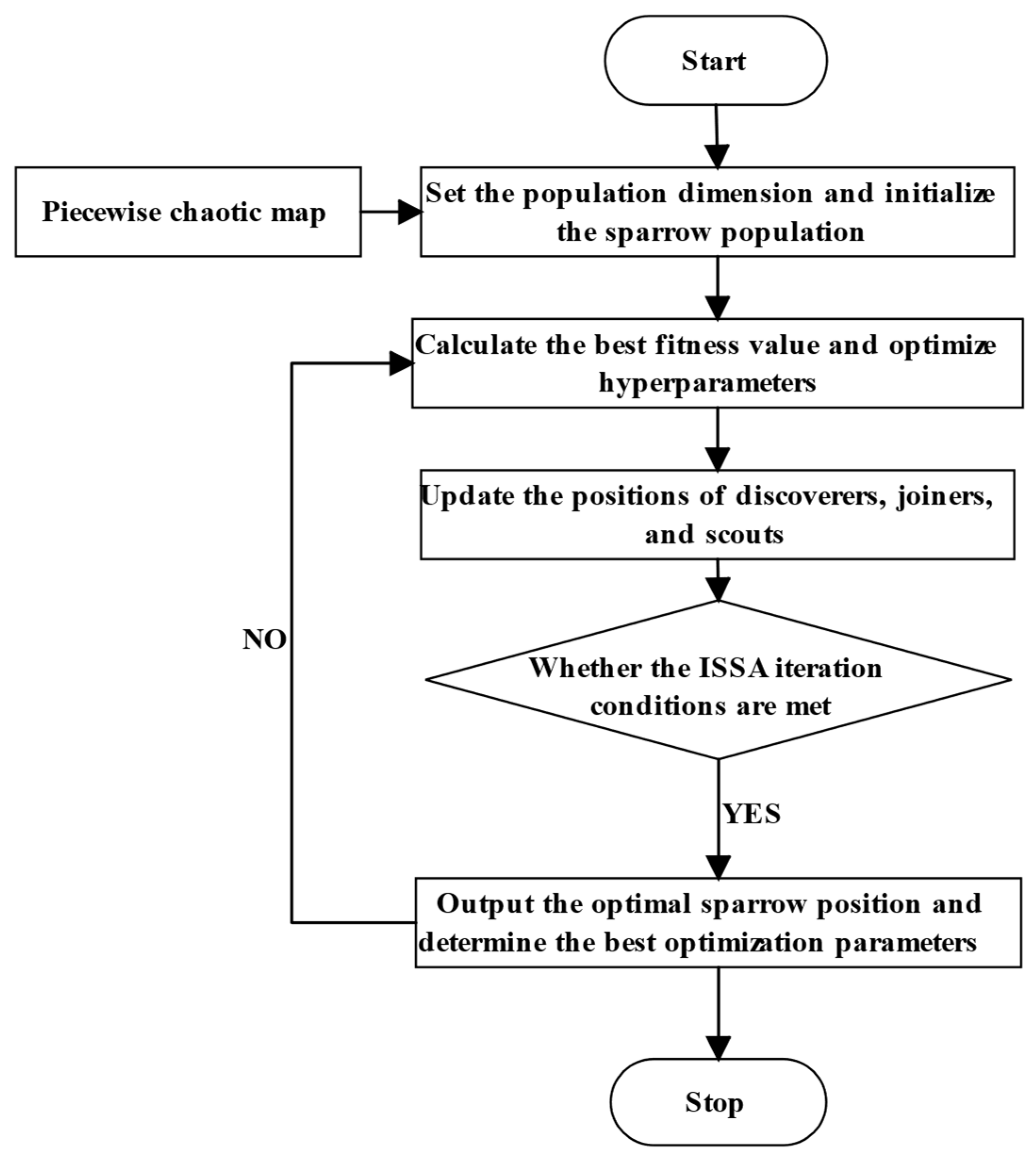
Additionally, the flowchart illustrating the process of utilizing the final ISSA to optimize the LSTM network parameters is depicted in Figure 2.

2.7. Testing the Performance of the ISSA Functions

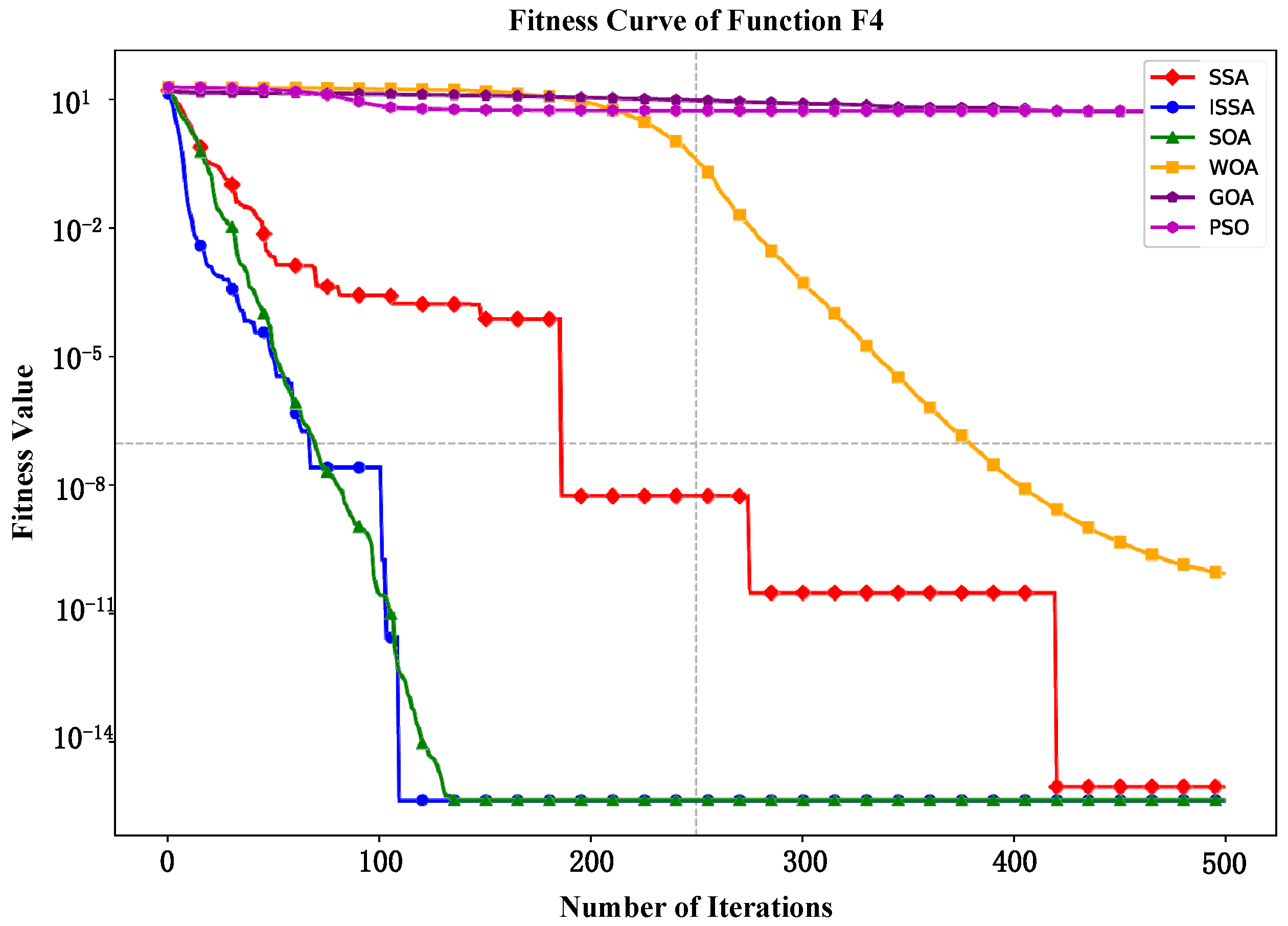
To intuitively demonstrate the overall performance of the Improved Sparrow Search Algorithm (ISSA), comparative experiments are conducted by comparing the ISSA with the Sparrow Search Algorithm (SSA), Seagull Optimization Algorithm (SOA), Whale Optimization Algorithm (WOA), Locust Optimization Algorithm (GOA), and Particle Swarm Optimization (PSO). In these experiments, the number of experimental populations is set as 30, and the iteration number is fixed at 500. The test function employed is defined in Equation (26) [32], with its relevant parameters listed in Table 2. Furthermore, the average fitness values of these algorithms (calculated as the mean of 30 independent iterations) are compared, as shown in Table 3.
Table 3 reveals that the ISSA demonstrates the optimal capability in locating the optimal value, locating the optimal solution with fewer iterations across all five functions. This indicates that the ISSA exhibits a stronger global search capability and faster convergence speed, which can be attributed to the introduction of improved chaotic mapping into the SSA population. This enhancement boosts the randomness and ergodicity of the population, enabling the better handling of local optima during both local exploitation and global search processes. The SSA and SOA rank next in terms of performance, whereas the WOA, GOA, and PSO show relatively inferior results. Therefore, in Example 2 of this study, comparative experiments are carried out employing the ISSA, SSA, and SOA to further explore their performance discrepancies.
Figure 3 and Figure 4, respectively, depict the fitness curves of the unimodal function F 2 and the multimodal function F 4 . When subjected to the same number of iterations, the ISSA demonstrates superiority by being the first to converge to the optimal fitness value.
F 1 = i = 1 n x i 2 F 2 = i = 1 n x i + i = 1 n x i F 3 = i = 1 n x i 2 10 cos 2 π x i + 10 F 4 = 20 exp 0.2 1 n i = 1 n x i 2 exp 1 n i = 1 n cos 2 π x i + 20 + e F 5 = 4 x 1 2 2.1 x 1 4 + 1 3 x 1 6 + x 1 x 2 4 x 2 2 + 4 x 2 4

3. Structure of Prediction Model

Currently, electric power load data, influenced by diverse factors such as meteorological conditions and user behavioral patterns, exhibit prominent nonlinearity and volatility. These characteristics impose stringent demands on the construction of forecasting models. Therefore, through a comprehensive exploration of data features and the implementation of precise data-fitting strategies, the prediction accuracy can be effectively enhanced.
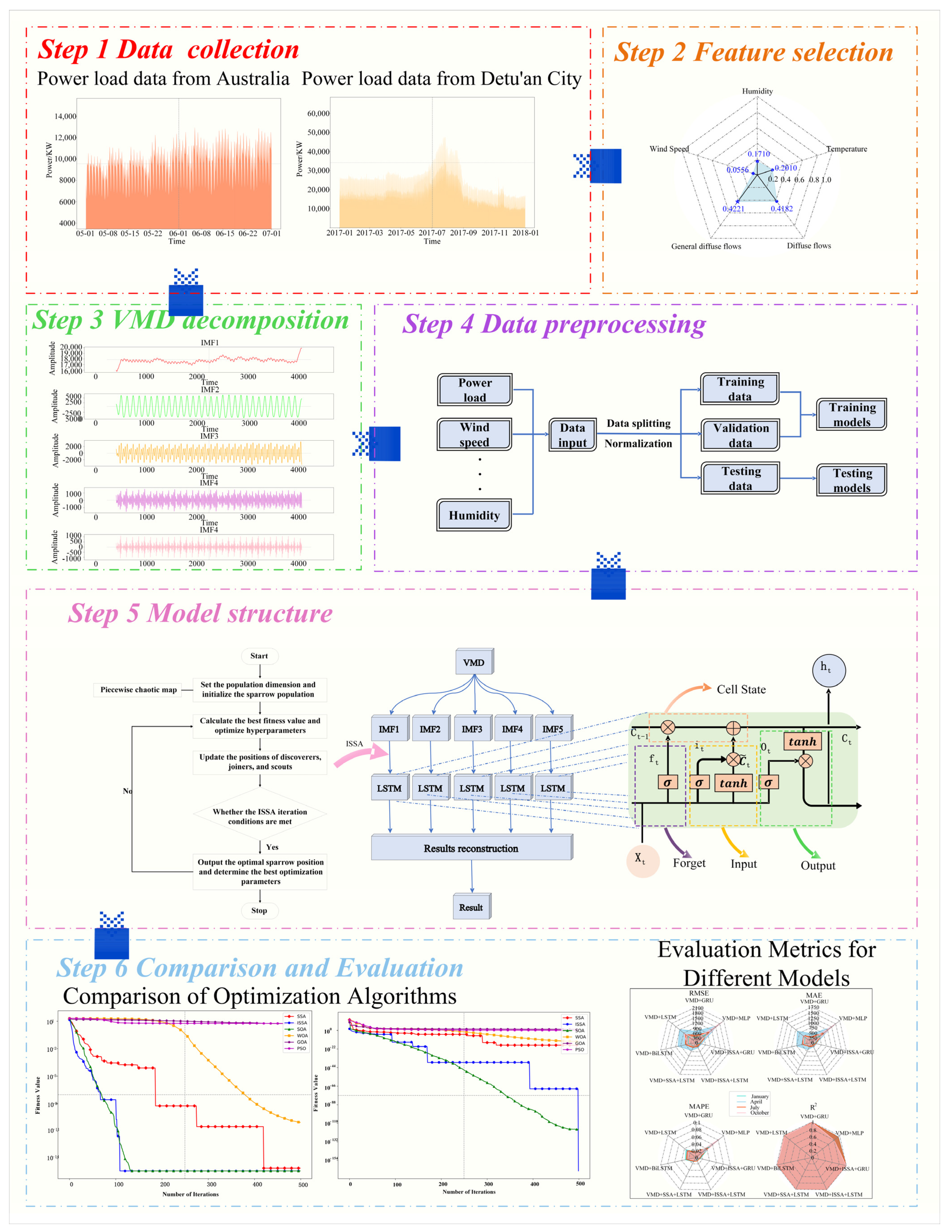
This paper presents a data-driven hierarchical framework for short-term power load forecasting. The methodology begins with Variational Mode Decomposition (VMD) to decompose the original load series into intrinsic mode functions (IMFs). Permutation entropy (PE) is used to determine the optimal decomposition mode number   K , which quantifies the time-series complexity for optimal decomposition. Concurrently, the Maximum Information Coefficient (MIC) is employed to mine the latent characteristics between the meteorological data (e.g., temperature and humidity) and load values, serving to filter more suitable input features for the prediction model. Subsequently, the filtered meteorological features are reconstructed with the decomposed load components (IMFs) and jointly fed into a Long Short-Term Memory (LSTM) network for prediction. To mitigate subjective hyperparameter tuning, the Improved Sparrow Search Algorithm (ISSA) adaptively optimizes three critical LSTM parameters: the learning rate l r to govern weight updates, hidden layer neuron counts L to balance the model capacity, and the training batch size N to stabilize the gradient estimation. Finally, the predicted results from LSTM are summed and reconstructed to obtain the final predicted data. This framework systematically addresses the load data’s nonlinearity and volatility by combining VMD’s multi-scale decomposition, the ISSA’s bio-inspired optimization, and LSTM’s sequence modeling.
In this paper, we first decompose the original load into a set of intrinsic modal components by VMD and use permutation entropy to determine the optimal decomposition model number K. Then, we input each component and the reconstruction of meteorological factors into the LSTM network as input features for prediction, and, at the same time, we optimize the hyperparameters of the LSTM model by using the ISSA, so as to reduce the effects of subjective factors and a priori knowledge and, thus, better capture the sequence. At the same time, the ISSA is used to optimize the hyperparameters of the LSTM model to reduce the influence of subjective factors and a priori knowledge, so as to better capture the sequence pattern and improve the prediction accuracy; finally, the results are reconstructed to obtain the final prediction results. The overall hierarchical framework of the ISSA-optimized VMD-LSTM short-term power load forecasting is shown in Figure 5.

4. Performance Indicators

In this study, four performance metrics are employed to evaluate the prediction accuracy of the proposed model: the root mean square error E R M S E , the mean absolute error E M A E , the mean absolute percentage error E M A P E , and the coefficient of determination R 2 . The mathematical definitions are given by
E R M S E = t = 1 N y t y ^ t 2 N
E M A E = t = 1 N y t y ^ t N
E M A P E = t = 1 N y t y ^ t y t N × 100 %
R 2 = 1 t = 1 N y t y ^ t 2 t = 1 N y t y ¯ t 2
where N represents the number of samples, and y t , y ^ t , and y ¯ t denote the true value, predicted value, and average value of the data at time t , respectively. For E R M S E , E M A E , and E M A P E , smaller values signify a higher prediction accuracy, and all these metrics fall within the range of 0,1 . A value of R 2 closer to unity indicates that the fit is better.

5. Experiment and Analysis

5.1. Data Description and Preprocessing

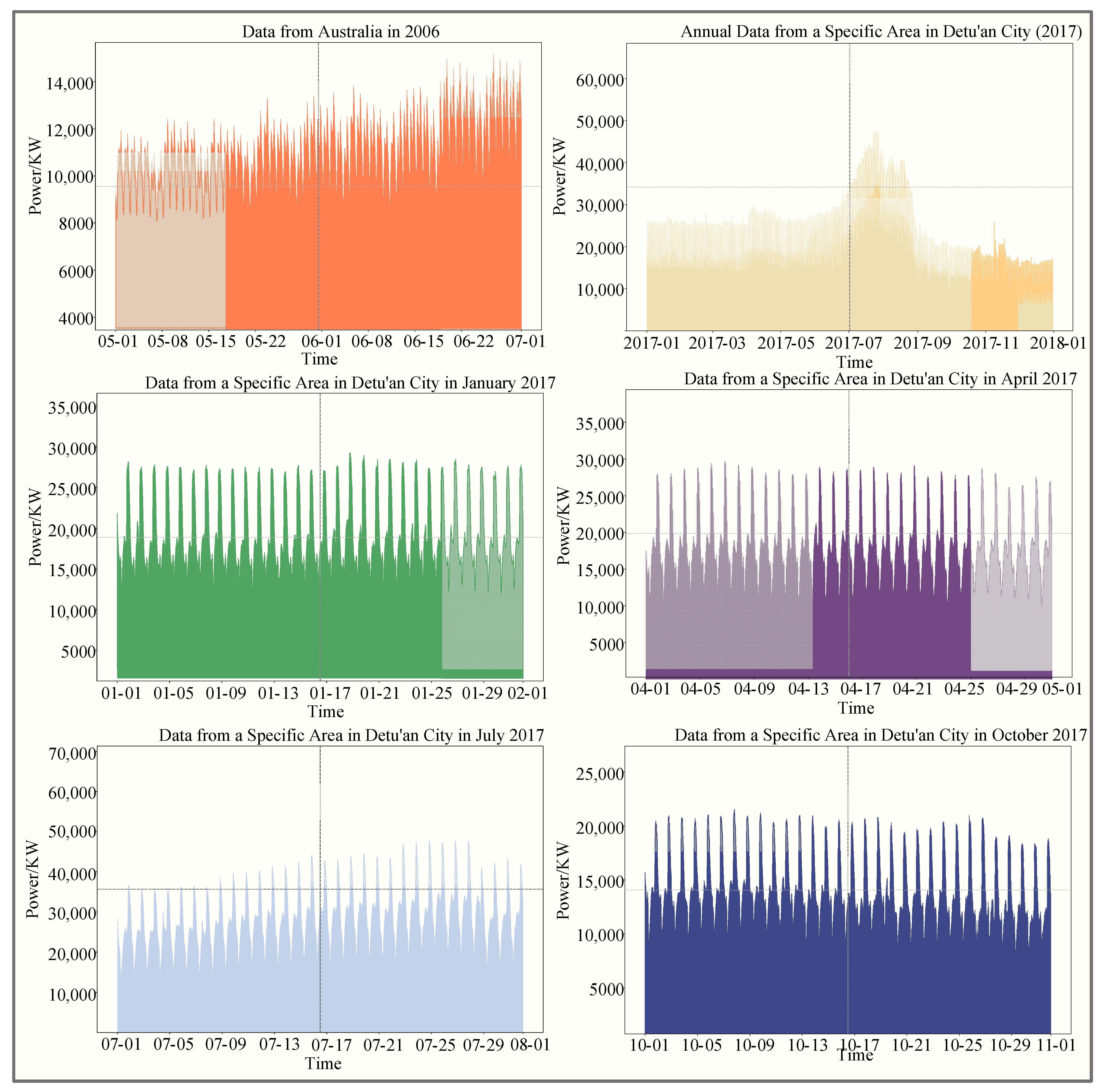
To validate the superiority of the proposed model, historical data from Tetuan City and a region in Australia were selected for empirical analysis. For Detu’an City, data from January, April, July, and October 2017—encompassing six characteristics (e.g., temperature, humidity, and load)—were utilized to validate seasonal patterns, with measurements recorded every 10 min (144 data points per day) and a total of 17,712 data points. Meanwhile, to address challenges like overfitting and the excessive data similarity in the forecasting process, two months of data from Australia (i.e., May–June 2006 data), covering features such as load and humidity, were adopted for validation. These data were sampled at 30 min intervals (48 data points per day), yielding a total of 2928 data points. The raw data are presented in Figure 6.
Moreover, models like the GRU and LSTM, alongside optimization algorithms such as the SSA and SOA, are employed for the comparative analysis with the proposed model. This comparative experiment serves to validate the proposed model’s superior prediction accuracy. Furthermore, predictions using data from distinct regions are produced, which in turn verifies the model’s excellent generalization capability across varied datasets.
In this study, the experimental hardware platform is equipped with the 12th Gen Intel (R) Core (TM) i5-12450H CPU. For software configuration, the experiments are executed in the Python 3.8 environment, and the deep learning models are developed using the Pytorch and Tensorflow frameworks.
For the data preprocessing process, as the data in this paper are acquired via continuous sampling, the Hampel filtering method is mainly utilized to address data outliers—detected outliers are filled with the median value. To improve the model’s convergence and ensure that the input data have consistent scales, Max–Min normalization is performed. Lastly, inverse normalization is applied to the predicted values to derive the final forecasting results.

5.2. Parameter Settings

In this study, the Variational Mode Decomposition (VMD) is configured with a penalty parameter of α = 1300 to balance the bandwidth constraint strength and decomposition fidelity and a noise tolerance parameter of τ = 0 to enforce noise-free decomposition. The number of decomposition modes K is adaptively determined via permutation entropy analysis, which quantifies the time-series complexity for an optimal decomposition. Other parameters follow the original VMD formulation: DC offset D C = 0 , initial mode functions i n i t = 1 , and iteration convergence tolerance t o l = 10 7 .
To validate the proposed model’s performance, comparative experiments were conducted using MLP, LSTM, and GRU models. The MLP adopted a basic configuration. The LSTM and GRU were configured with 64 units, respectively. All models shared common hyperparameters: a 0.2 dropout rate, MSE loss function, and Adam optimizer.
To ensure a fair comparison and validate the superiority of the proposed Improved Sparrow Search Algorithm (ISSA), a unified parameter configuration is adopted for optimization algorithms (ISSA, SSA, SOA), including the following: the population size N = 10 , iteration number T = 30 , alert value f a = 0.6 (triggering danger avoidance behavior), scout proportion λ = 0.7 (leading food source exploration), and danger-aware proportion p d = 0.2 (modeling threat recognition). Optimization algorithms are primarily employed to optimize the hyperparameters of the LSTM model, specifically targeting three critical variables, the learning rate l r [ 0.001,0.05 ] , the number of hidden layer neurons L [ 10,500 ] , and the training batch size N [ 100,1200 ] , to identify their optimal configurations.

5.3. Feature Selection

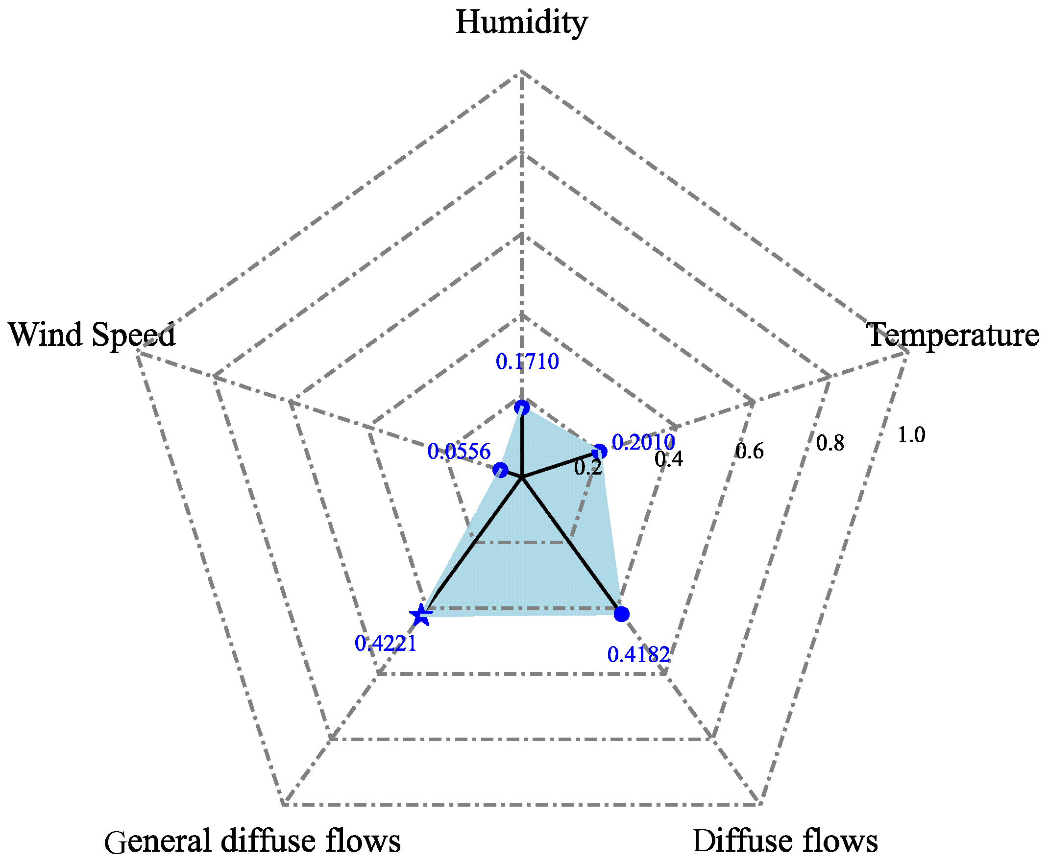
To fully exploit data features and enhance the prediction accuracy, this study employs the maximum mutual information coefficient for an adaptive input feature selection. Specifically, one-year data from a region in Tetuan City are used as a case study, with Figure 7 illustrating the mutual information coefficients between the electric load and candidate input features (e.g., temperature, humidity, and historical load).
In the figure, the star symbol denotes the feature with the highest correlation coefficient. Given the relatively low correlation between the wind speed and load, the remaining four features are selected as meteorological inputs to the model, as visualized by the circular markers in Figure 7.

5.4. Example 1 Experiment

To comprehensively validate the proposed method’s effectiveness in seasonal electric load forecasting, time-series data from a Tetuan City region were employed. For seasonal validation, mid-season months (January for winter, April for spring, July for summer, and October for autumn) were selected, aligning with typical peak or off-peak load patterns. The load data were collected at 10 min intervals to enable the fine-grained modeling of load dynamics, with the dataset partitioned into training (70%), validation (10%), and test (20%) sets using chronological partitioning. This configuration yields 3024 training samples, 432 validation samples, and 864 test samples per month, preserving temporal dependency for a realistic model evaluation.
(1) No VMD used
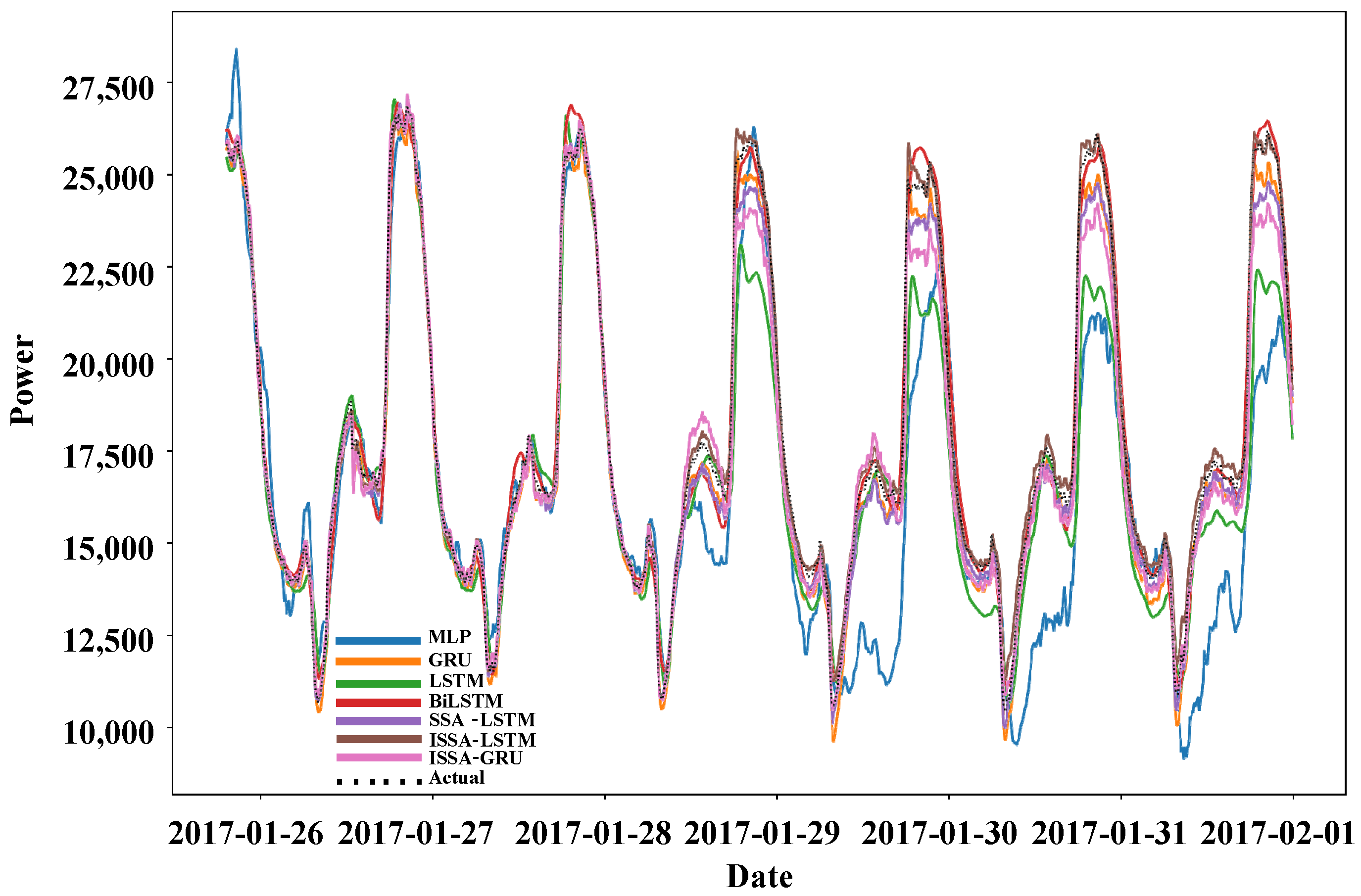
The January load forecasting results in Figure 8 demonstrate that the GRU and BiLSTM outperform the feedforward model and achieve a superior peak load prediction due to their temporal dependency modeling capability. Notably, the load curve exhibits the strongest volatility and most complex temporal features at peaks and valleys, where traditional forecasting methods often show a weak learning performance. The method proposed in this paper effectively addresses this limitation: integrating the Improved Sparrow Search Algorithm (ISSA) significantly enhances performance and the ISSA-LSTM reduces the E R M S E , E M A E , and E M A P E by 78.34%, 76.66%, and 72.24% compared to LSTM, as quantified in Table 4. The ISSA-LSTM prediction curve closely aligns with actual loads, particularly during diurnal peaks and nighttime valleys, attributed to the ISSA’s optimized hyperparameters. This optimization resolves the single LSTM’s weakness in capturing non-stationary features.
Compared with the SSA-LSTM model, the E M A P E of the ISSA-LSTM decreased by 28.77%, which indicates that the ISSA is better for LSTM hyperparameter optimization compared with the original SSA, which is because the ISSA is more uniform for population initialization, which effectively avoids falling into the local optimal solution and improves the ability of the global search of the population.
(2) VMD used
To avoid over-decomposition (causing modal aliasing or introducing spurious noise) and under-decomposition (resulting in insufficient data separation), the VMD mode number K is constrained within the range of 4–9. The relationship between the permutation entropy (PE) values of decomposed components and K is quantified in Table 5, where the optimal K is identified as the smallest integer minimizing PE while ensuring component stationarity.
As observed from Table 5, the mean permutation entropy (PE) of each decomposed load component reaches its minimum when the decomposition level reaches K = 5 . Permutation entropy, a measure of time-series complexity, quantifies the regularity of a sequence such that lower PE values indicate higher regularity, while higher PE values reflect greater complexity. Furthermore, excessive decomposition levels may introduce computational redundancy without improving interpretability. Considering the trade-off between sequence regularity and computational efficiency, the optimal decomposition number is determined to be K = 5 . The corresponding decomposition results of the load sequence are illustrated in Figure 9.
Table 6 demonstrates that the VMD-ISSA-LSTM and the VMD-ISSA-GRU outperform non-optimized counterparts by leveraging the ISSA for hyperparameter optimization. Specifically, the VMD-ISSA-LSTM achieves E M A P E reductions of 94.6%, 47.78%, 82.97%, and 78.73%, while the VMD-ISSA-GRU reduces the E M A P E by 93.22%, 34.44%, 78.62%, and 73.3%. These improvements are statistically significant, confirming the superiority of the ISSA-driven hyperparameter tuning.
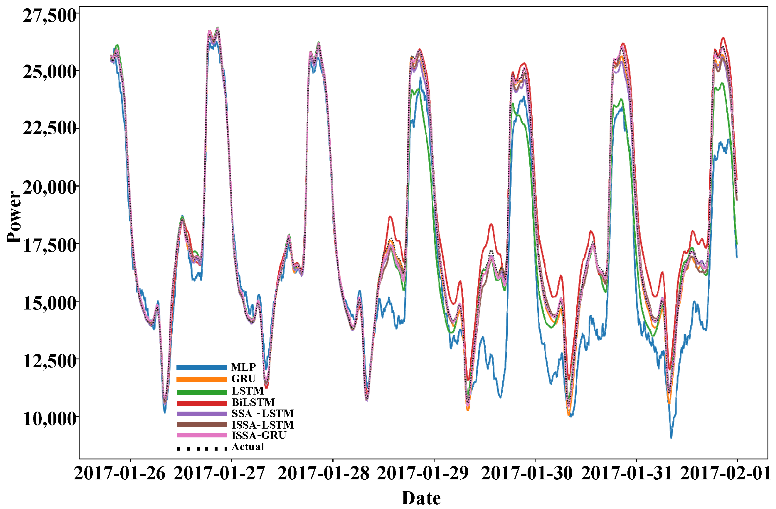
The visual inspection of the VMD results demonstrates a reduction in load complexity, as unprocessed load data directly used for prediction lead to significantly larger forecasting errors and increased prediction difficulty. By integrating Variational Mode Decomposition (VMD) with predictive models, the hybrid forecasting framework achieves an improved performance. Quantitative results are presented in Figure 10 and Table 6.
As can be seen from Table 6, the ISSA-LSTM and ISSA-GRU exhibit the most pronounced improvements, with the E M A P E reduced by 69.87% and 62.89%, respectively, compared to their non-decomposed baselines. These results statistically confirm that VMD significantly enhances the prediction accuracy across all tested models. Mechanistically, this improvement arises because VMD addresses the inherent volatility and non-stationarity of load sequences by decomposing them into intrinsic mode functions (IMFs) with distinct temporal scales. This decomposition mitigates the complexity of the prediction task by transforming non-stationary data into stationary sub-sequences, aligning with the time-frequency analysis principles of the mode decomposition family.
Table 6 reveals that the proposed method outperforms the VMD-ISSA-GRU with the E R M S E reduced by 25.67%, the   E M A E by 21.21%, and the E M A P E by 20.34%. This improvement is attributed to the architectural difference between LSTM and the GRU: the GRU merges the forget gate and input gate into a single update gate, potentially discarding critical long-term dependencies in complex decomposed load sequences. Although the VMD and ISSA optimization enhance the GRU’s performance, the GRU’s simplified gating mechanism limits its feature representation capacity for non-stationary intrinsic mode functions (IMFs), leading to a suboptimal hyperparameter tuning compared to the LSTM-based architecture.
Table 6 quantitatively validates that the proposed ISSA-based method outperforms VMD-SSA-LSTM, with the E R M S E reduced by 55.56%, the E M A E by 53.19%, and the E M A P E by 45.98%. These improvements significantly surpass the SSA-based baseline, confirming the effectiveness of the ISSA in addressing the SSA’s inherent limitations (e.g., premature convergence and suboptimal parameter exploration).
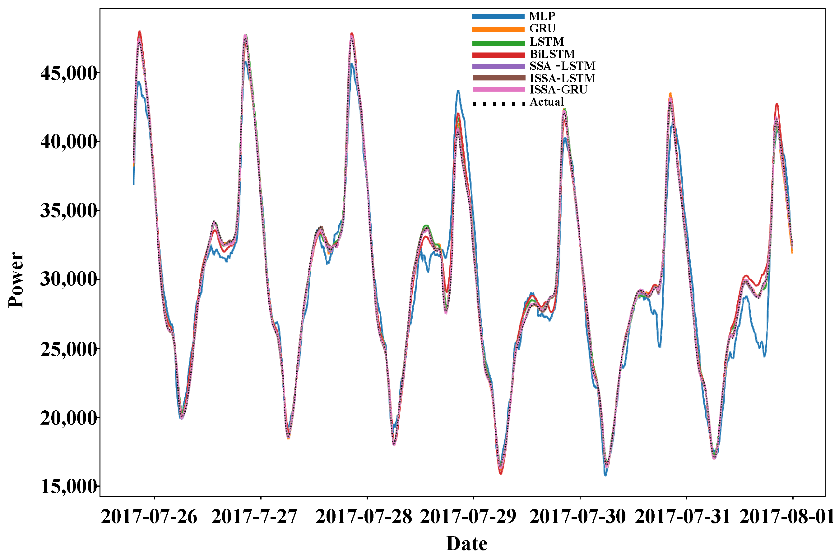
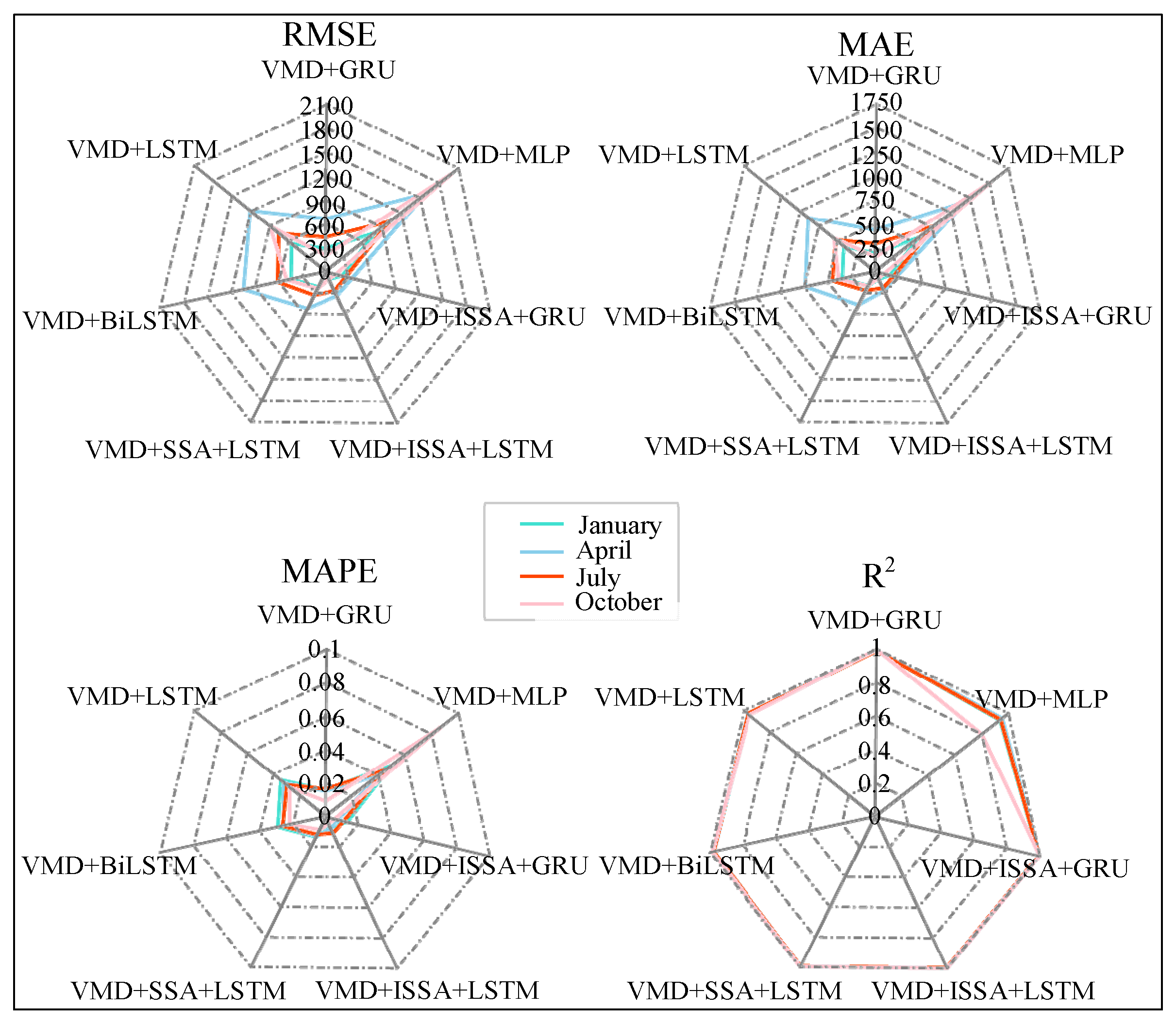
To further validate the generalizability of the proposed method, out-of-sample prediction experiments were conducted using the April, July, and October load profiles (Figure 11, Figure 12 and Figure 13). Quantitative error metrics (Table 7) and visual comparisons collectively demonstrate that the ISSA-optimized GRU and LSTM models outperform non-optimized baselines. Specifically, the ISSA-enhanced architectures achieve a superior fitting performance across all test months, with notable improvements in capturing load peaks and valleys (e.g., July peak load prediction error reduced by 31.2% vs. non-optimized LSTM).
To further validate the generalizability of the proposed method, other months are used for prediction. The comparisons of the prediction results for April, July, and October are shown in Figure 11, Figure 12 and Figure 13, respectively, and the comparison of the errors is shown in Table 7. Specifically, the ISSA-enhanced architectures achieve a superior fitting performance across all test months, with notable improvements in capturing load peaks and valleys. This indicates that the improved model proposed in this paper has certain advantages.
The comparative analysis of the prediction performance demonstrates that applying Variational Mode Decomposition (VMD) significantly enhances the forecasting accuracy for the regional power load in Tetuan City compared to direct prediction methods without decomposition. This improvement primarily stems from VMD’s capability to effectively decompose complex load signals into relatively stable intrinsic mode functions (IMFs), thereby extracting essential temporal features while reducing the data complexity through adaptive noise reduction. As illustrated in Figure 14, the forecasting accuracy exhibits notable seasonal variations, with January and October demonstrating superior prediction performances compared to April and July.
The observed forecasting discrepancies can be attributed to distinct seasonal characteristics: April represents a transitional period between spring and summer characterized by significant temperature volatility and abrupt increases in cooling demands. This meteorological instability, combined with altered consumption patterns during public holidays (e.g., Tomb-Sweeping Day), results in substantial deviations from typical load profiles.
July presents unique forecasting challenges as the peak summer month, where extreme heat events drive cooling loads beyond conventional projections. Concurrently, industrial load patterns become less predictable due to strategic load-shifting measures implemented by energy-intensive enterprises and potential power rationing during grid stress conditions. These operational adaptations create short-term load distribution anomalies that conventional forecasting models struggle to capture effectively.

5.5. Example 2 Experiment

To further validate the model’s generalizability, out-of-sample experiments were conducted using the May 2006 (final spring month) and June 2006 (initial summer month) load data from an Australian region.
In order to further verify the strong generalization ability of the model, the data of the last month of spring (May) and the first month of summer (June) in an area of Australia in 2006 were selected for experimental verification. According to the decomposition results of Example 1, this example uses VMD for the experiment. Since the prediction effect of MLP is worse than that of LSTM and the GRU, this example uses the GRU, BiLSTM, and other models as comparison algorithms. In addition, this experiment also introduces the SOA to compare with the ISSA, aiming to further highlight the advantages of the ISSA.
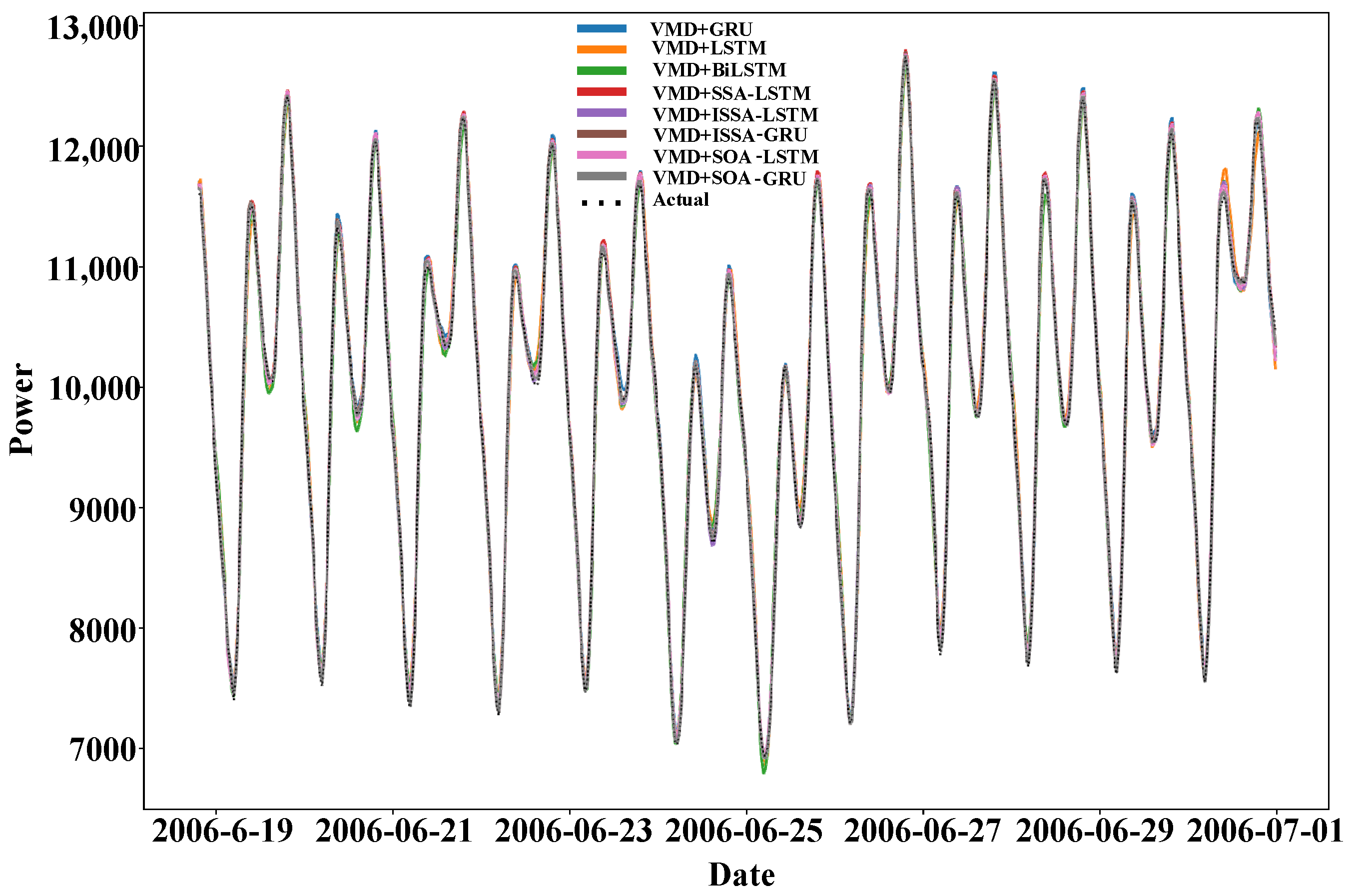
The comparison of the prediction results of a regional model in Australia is shown in Figure 15. As can be seen from the figure, compared with the method of single fusion VMD, the method that added an optimization algorithm to optimize model hyperparameters has a relatively better prediction effect and higher prediction accuracy. Since the load data of two months are used in the experiment in this example, the data volume is larger than that of Example 1, and the model proposed in this paper can extract data features more fully and capture the nonlinear relationship of the load sequence, which has a better fitting effect on the trend of the load data and a higher prediction accuracy.
The prediction error indicators of each model are shown in Table 8. It can be seen from the table that models using the ISSA and GRU optimization algorithms have better prediction effects than models such as the GRU and LSTM, among which VMD+ISA-LSTM has a particularly prominent prediction effect. Compared with other models, such as the GRU and LSTM, the E R M S E decreases by 55.53%, 73.93%, 70.23%, 43.85%, 8.63%, 10.73%, and 41.14%, respectively. The prediction of different regional data proves that the proposed model has a high prediction accuracy and good generalization performance.
At the same time, by comparing the ISSA’s optimization algorithm with the SOA’s optimization algorithm, it can be seen that the ISSA has a better prediction effect, among which, the E R M S E of VMD+ISA-LSTM and VMD+SOA-LSTM and VMD+SOA-GRU are decreased by 10.73% and 41.14%, respectively. The E R M S E of VMD+ISA-GRU decreased by 2.3% and 35.58% compared with VMD+SOA-LSTM and VMD+SOA-GRU.
Through the comparison between the ISSA and SOA in practical cases, the models optimized by the ISSA exhibit lower RMSE values and better prediction performances, further demonstrating the robustness and generalization ability of the ISSA.

6. Conclusions

To tackle the challenges of the inadequate adaptability to non-stationarity and poor precision in capturing nonlinear characteristics inherent in traditional short-term power load forecasting methods, this paper proposes a novel forecasting model based on the Improved Sparrow Search Algorithm (ISSA). The key contributions are summarized as follows:
(1) The model decomposition of load sequences is conducted via Variational Mode Decomposition (VMD). This approach effectively resolves the mode mixing issue commonly found in decompositions like Empirical Mode Decomposition (EMD), decomposing nonlinear and fluctuating data into stable, regular subsequences with clear physical meanings.
(2) Permutation entropy is employed to determine the optimal number of decomposition modes, which improves the accuracy and efficiency of the signal decomposition, ensures optimal decomposition, enhances decomposition precision, and optimizes the prediction performance.
(3) The Long Short-Term Memory (LSTM) network is utilized to integrate decomposed sequences with meteorological factors for prediction. This approach effectively extracts the temporal characteristics and complex nonlinear relationships of load data, thereby fully excavating data characteristics and improving the prediction accuracy compared to other models.
(4) The ISSA is adopted to optimize the hyperparameters of LSTM. Compared with other algorithms, the ISSA optimization algorithm used in this study features a lower complexity and achieves a better optimization performance. Minimizing the influence of subjective factors and prior knowledge, this optimization achieves the best prediction performance of the VMD-LSTM framework.
In summary, the method proposed in this paper has a greater precision and better generalization performance for short-term power load forecasting. In future research, we can consider using data from different industries for forecasting, selecting more efficient models and optimization algorithms, or conducting forecasting research for loads affected by emergencies, so as to further improve the forecasting performance of the model.

Author Contributions

Conceptualization, S.W. and H.C.; methodology, S.W.; software, S.W.; validation, S.W. and H.C.; formal analysis, S.W. and H.C.; investigation, S.W. and H.C.; data curation, S.W.; writing—original draft preparation, S.W. and H.C.; writing—review and editing, S.W. and H.C.; visualization, S.W.; supervision, H.C.; project administration, H.C.; funding acquisition, S.W. and H.C. All authors have read and agreed to the published version of the manuscript.

Funding

This research was partially funded by the Innovation Fund for Industry-University-Research in Chinese Universities (2024HY031).

Institutional Review Board Statement

Not applicable.

Informed Consent Statement

Not applicable.

Data Availability Statement

Publicly available datasets were analyzed for this study. Example 1 can be found here: https://archive.ics.uci.edu/dataset/849/power+consumption+of+tetouan+city (accessed on 11 February 2025). Example 2 can be found here: https://gitcode.com/qq_42998340/Australia.

Acknowledgments

The authors are deeply obliged to the anonymous reviewers and editor for their insightful comments and constructive feedback.

Conflicts of Interest

The authors declare no conflicts of interest.

References

  1. Raza, M.Q.; Khosravi, A. A review on artificial intelligence based load demand forecasting techniques for smart grid and buildings. Renew. Sustain. Energy Rev. 2015, 50, 1352–1372. [Google Scholar] [CrossRef]
  2. Mi, J.; Fan, L.; Duan, X.; Qiu, Y. Short-term power load forecasting method based on improved exponential smoothing grey model. Math. Probl. Eng. 2018, 2018, 3894723. [Google Scholar] [CrossRef]
  3. Li, J.; Deng, D.; Zhao, J.; Cai, D.; Hu, W.; Zhang, M.; Huang, Q. A novel hybrid short-term load forecasting method of smart grid using MLR and LSTM neural network. IEEE Trans. Ind. Inform. 2020, 17, 2443–2452. [Google Scholar] [CrossRef]
  4. Yang, Z.; Ce, L.; Lian, L. Electricity price forecasting by a hybrid model, combining wavelet transform, ARMA and kernel-based extreme learning machine methods. Appl. Energy 2017, 190, 291–305. [Google Scholar] [CrossRef]
  5. Shi, H.; Xu, M.; Li, R. Deep learning for household load forecasting—A novel pooling deep RNN. IEEE Trans. Smart Grid 2017, 9, 5271–5280. [Google Scholar] [CrossRef]
  6. Chang, Z.; Zhang, Y.; Chen, W. Electricity price prediction based on hybrid model of adam optimized LSTM neural network and wavelet transform. Energy 2019, 187, 115804. [Google Scholar] [CrossRef]
  7. Lv, L.; Wu, Z.; Zhang, J.; Zhang, L.; Tan, Z.; Tian, Z. A VMD and LSTM based hybrid model of load forecasting for power grid security. IEEE Trans. Ind. Inform. 2021, 18, 6474–6482. [Google Scholar] [CrossRef]
  8. Zhang, X.; Chau, T.K.; Chow, Y.H.; Fernando, T.; Iu, H.H.C. A novel sequence to sequence data modelling based CNN-LSTM algorithm for three years ahead monthly peak load forecasting. IEEE Trans. Power Syst. 2023, 39, 1932–1947. [Google Scholar]
  9. Li, C.; Tang, G.; Xue, X.; Saeed, A.; Hu, X. Short-term wind speed interval prediction based on ensemble GRU model. IEEE Trans. Sustain. Energy 2019, 11, 1370–1380. [Google Scholar] [CrossRef]
  10. Gao, X.; Li, X.; Zhao, B.; Ji, W.; Jing, X.; He, Y. Short-term electricity load forecasting model based on EMD-GRU with feature selection. Energies 2019, 12, 1140. [Google Scholar] [CrossRef]
  11. Chiu, M.C.; Hsu, H.W.; Chen, K.S.; Wen, C.Y. A hybrid CNN-GRU based probabilistic model for load forecasting from individual household to commercial building. Energy Rep. 2023, 9, 94–105. [Google Scholar] [CrossRef]
  12. Pang, S.; Zou, L.; Zhang, L.; Wang, H.; Wang, Y.; Liu, X.; Jiang, J. A hybrid TCN-BiLSTM short-term load forecasting model for ship electric propulsion systems combined with multi-step feature processing. Ocean Eng. 2025, 316, 119808. [Google Scholar] [CrossRef]
  13. Xu, H.; Fan, G.; Kuang, G.; Song, Y. Construction and application of short-term and mid-term power system load forecasting model based on hybrid deep learning. IEEE Access 2023, 11, 37494–37507. [Google Scholar] [CrossRef]
  14. Zou, Z.; Wang, J.; Ning, E.; Zhang, C.; Wang, Z.; Jiang, E. Short-term power load forecasting: An integrated approach utilizing variational mode decomposition and TCN–BiGRU. Energies 2023, 16, 6625. [Google Scholar] [CrossRef]
  15. Wang, Y.; Guo, P.; Ma, N.; Liu, G. Robust wavelet transform neural-network-based short-term load forecasting for power distribution networks. Sustainability 2022, 15, 296. [Google Scholar] [CrossRef]
  16. Wu, Y.; Cong, P.; Wang, Y. Charging load forecasting of electric vehicles based on VMD-SSA-SVR. IEEE Trans. Transp. Electrif. 2023, 10, 3349–3362. [Google Scholar] [CrossRef]
  17. Li, S.; Cai, H. Short-Term Power Load Forecasting Using a VMD-Crossformer Model. Energies 2024, 17, 2773. [Google Scholar] [CrossRef]
  18. Tang, Y.; Cai, H. Short-term power load forecasting based on vmd-pyraformer-adan. IEEE Access 2023, 11, 61958–61967. [Google Scholar] [CrossRef]
  19. Sun, Q.; Cai, H. Short-term power load prediction based on VMD-SG-LSTM. IEEE Access 2022, 10, 102396–102405. [Google Scholar] [CrossRef]
  20. Liu, J.; Cong, L.; Xia, Y.; Pan, G.; Zhao, H.; Han, Z. Short-term power load prediction based on DBO-VMD and an IWOA-BILSTM neural network combination model. Power Syst. Prot. Control 2024, 52, 123–133. [Google Scholar]
  21. Mounir, N.; Ouadi, H.; Jrhilifa, I. Short-term electric load forecasting using an EMD-BI-LSTM approach for smart grid energy management system. Energy Build. 2023, 288, 113022. [Google Scholar] [CrossRef]
  22. Deng, D.; Li, J.; Zhang, Z.; Teng, Y.; Huang, Q. Short-term Electric Load Forecasting Based on EEMD-GRU-MLR. Power Syst. Technol. 2020, 44, 593–602. [Google Scholar] [CrossRef]
  23. Ding, Y.; Chen, Z.; Zhang, H.; Wang, X.; Guo, Y. A short-term wind power prediction model based on CEEMD and WOA-KELM. Renew. Energy 2022, 189, 188–198. [Google Scholar] [CrossRef]
  24. Liu, J.; Jin, Y.; Tian, M. Multi-Scale Short-Term Load Forecasting Based on VMD and TCN. J. Univ. Electron. Sci. Technol. China 2022, 51, 550–557. [Google Scholar] [CrossRef]
  25. Wang, X.; Sun, N.; Su, H.; Zhang, N.; Zhang, S.; Ji, J. Ultra-short-term wind speed prediction based on sample entropy-based dual decomposition and ssa-lstm. Acta Energiae Solaris Sin. 2025, 46, 611–618. [Google Scholar]
  26. Zhang, H.; He, S. Analysis and comparison of permutation entropy, approximate entropy and sample entropy. In Proceedings of the 2018 International Symposium on Computer, Consumer and Control (IS3C), Taichung, Taiwan, 6–8 December 2018; IEEE: Piscataway, NJ, USA, 2018; pp. 209–212. [Google Scholar]
  27. Reshef, D.N.; Reshef, Y.A.; Finucane, H.K.; Grossman, S.R.; McVean, G.; Turnbaugh, P.J.; Lander, E.S.; Mitzenmacher, M.; Sabeti, P.C. Detecting novel associations in large data sets. Science 2011, 334, 1518–1524. [Google Scholar] [CrossRef] [PubMed]
  28. Kinney, J.B.; Atwal, G.S. Equitability, mutual information, and the maximal information coefficient. Proc. Natl. Acad. Sci. USA 2014, 111, 3354–3359. [Google Scholar] [CrossRef]
  29. Yao, W.-P.; Liu, T.-B.; Dai, J.-F.; Wang, J. Multiscale permutation entropy analysis of electroencephalogram. Acta Phys. Sin. 2014, 63, 078704. [Google Scholar] [CrossRef]
  30. Xue, J.; Shen, B. A novel swarm intelligence optimization approach: Sparrow search algorithm. Syst. Sci. Control Eng. 2020, 8, 22–34. [Google Scholar] [CrossRef]
  31. Tang, Y.; Li, C.; Song, Y.; Chen, C.; Cao, B. Adaptive mutation sparrow search optimization algorithm. J. Beijing Univ. Aeronaut. Astronaut. 2023, 49, 681–692. (In Chinese) [Google Scholar] [CrossRef]
  32. Yang, H.Z.; Tian, F.M.; Zhang, P. Short-term load forecasting based on CEEMD-FE-AOA-LSSVM. Power Syst. Prot. Control 2022, 50, 126–133. [Google Scholar]
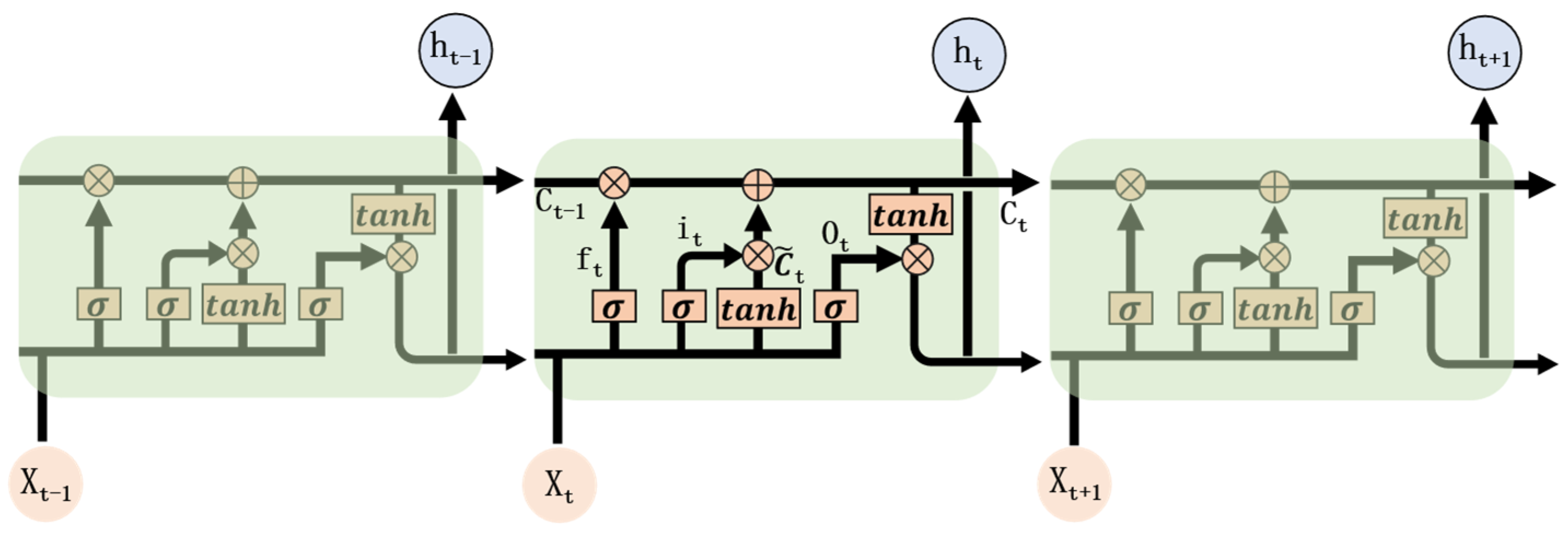
Figure 1. LSTM network structure diagram.
Applsci 15 05037 g001
Figure 2. Flowchart for optimizing LSTM network parameters using ISSA.
Applsci 15 05037 g002
Figure 3. Unimodal function fitness curves.
Applsci 15 05037 g003
Figure 4. Multimodal function fitness curves.
Applsci 15 05037 g004
Figure 5. Overall frame diagram. In Step 3, each color represents a different modal graph obtained from the decomposition. In Step 6, the red curve represents the Singular Spectrum Analysis (SSA) algorithm, the blue curve represents the Improved Singular Spectrum Analysis (ISSA) algorithm, the green curve represents the Sine Cosine Optimization Algorithm (SOA), the yellow curve represents the Whale Optimization Algorithm (WOA), the purple curve represents the Grasshopper Optimization Algorithm (GOA), and the pink curve represents the Particle Swarm Optimization (PSO) algorithm.If you have any further questions, please notify me in a timely manner.
Applsci 15 05037 g005
Figure 6. The raw data from Tetuan City and a region in Australia. The orange color represents the load data of a certain region in Australia from May to July 2006. The yellow color represents the load data of the city of Dushanbe throughout the whole year from 2017 to 2018. The green color represents the load data of Dushanbe in January. The purple color represents the load data of Dushanbe in April. The light blue color represents the load data of Dushanbe in July. The dark blue color represents the load data of Dushanbe in October.
Applsci 15 05037 g006
Figure 7. Correlation coefficient plot.
Applsci 15 05037 g007
Figure 8. Comparison of forecast results for January.
Applsci 15 05037 g008
Figure 9. The VMD results.
Applsci 15 05037 g009
Figure 10. Comparison of prediction results usin VMD in January.
Applsci 15 05037 g010
Figure 11. Comparison of April forecasts.
Applsci 15 05037 g011
Figure 12. Comparison of July forecasts.
Applsci 15 05037 g012
Figure 13. Comparison of October forecasts.
Applsci 15 05037 g013
Figure 14. Evaluation indicators of Tetuan City in four months.
Applsci 15 05037 g014
Figure 15. Comparison of model prediction results of region in Australia.
Applsci 15 05037 g015
Table 1. Review of related methods’ forecasting work.
ReferenceModelLimitationsOptimization
Wang Y, Guo P et al. [15]Wavelet Transform-LSTMManually adjust the model parametersNo
Mounir N, Ouadi H et al. [21]EMD-BiLSTMHigh computational cost, modal aliasingNo
DENG Daiyu, LI Jian et al. [22]EEMD-GRU-MLRResidual noiseNo
Ding Y, Chen Z, Zhang H et al. [23]CEEMD-WOA-KELMProne to local optima, sensitive to initial parametersYes
LIU Jie, JIN Yongjie et al. [24]VMD-TCN- Multi-ScaleComplex preprocessing, high implementation requirementsNo
Table 2. Test functions and their related parameters.
FunctionDefinitionMinimum Value
Unimodal function F 1 [−100,100]0
F 2 [−10,10]0
Multimodal function F 3 [−5.12,5.12]0
F 4 [−32,32]0
F 5 [−5,5]−1.0316
Table 3. Data comparison of algorithms.
FunctionAlgorithms
ISSASSASOAWOAGOAPSO
F 1 03.44 × 10−573.6 × 10−1946.01 × 10−2035.88710.1803
F 2 2.9 × 10−1673.12 × 10−188 × 10−1186.18 × 10−1420.81361.5318
F 3 0008.88 × 10−1697.592325.2767
F 4 4.44 × 10−169.18 × 10−164.44 × 10−168.92 × 10−115.48985.7464
F 5 −1.0316−1.0314−1.0316−1.0318−1.0318−1.0319
Table 4. No VMD used.
ModelRMSEMAEMAPER2
MLP2507.2451750.5570.09640.6881
GRU595.862481.4330.02750.9824
LSTM1618.6411081.2960.05620.87
BiLSTM614.801457.1150.02880.9811
SSA-LSTM568.124413.670.02190.984
ISSA-LSTM350.546252.3630.01560.9939
ISSA-GRU378.244284.7210.01590.9929
Table 5. The value of the entropy of each component.
K456789
mean0.95710.95460.99641.03141.061.0954
Table 6. Prediction results using the VMD.
ModelRMSEMAEMAPER2
VMD+MLP2001.7931526.2950.0870.7991
VMD+GRU194.987150.360.0090.9981
VMD+LSTM901.112552.2690.02760.9593
VMD+BiLSTM501.163386.7880.02210.9875
VMD-SSA-LSTM236.234168.4520.00870.9972
VMD+ISSA-LSTM104.98278.8480.00470.9994
VMD+ISSA-GRU141.247100.0780.00590.999
Table 7. Prediction error index of each model in April, July, and October.
SeasonAprilJulyOctober
ModelRMSEMAEMAPERMSEMAEMAPERMSEMAEMAPE
VMD+MLP1018.263770.780.04511584.6041186.170.0402781.282574.3610.0498
VMD+GRU430.194291.5290.0164663.289433.0220.0153287.508188.9090.0156
VMD+LSTM754.787526.3240.02991212.44891.9080.0322550.135417.8190.0346
VMD+BiLSTM614.344452.810.02631047.672740.1270.0258444.559347.5240.0292
VMD+SSA+LSTM329.864221.7140.0119516.604389.0360.0131214.702164.8940.0135
VMD+ISSA-LSTM267.966191.3030.0109337.4062220.008107.45287.6680.0072
VMD+ISSA-GRU269.221200.7410.0114348.445229.2630.008223.079161.5350.0135
Table 8. Prediction error index of each model.
ModelRMSEMAEMAPER2
VMD+GRU64.96452.3560.00530.9977
VMD+LSTM110.8488.0780.00890.9933
VMD+BiLSTM97.05276.8390.00780.9949
VMD+SSA-LSTM51.45742.2980.00430.9986
VMD+ISSA-LSTM28.89223.5270.00240.9995
VMD+ISSA-GRU31.6226.010.00260.9995
VMD+SOA-LSTM32.36626.2740.00260.9994
VMD+SOA-GRU49.08240.3030.00410.9987
Disclaimer/Publisher’s Note: The statements, opinions and data contained in all publications are solely those of the individual author(s) and contributor(s) and not of MDPI and/or the editor(s). MDPI and/or the editor(s) disclaim responsibility for any injury to people or property resulting from any ideas, methods, instructions or products referred to in the content.