Forecasting Models and Genetic Algorithms for Researching and Designing Photovoltaic Systems to Deliver Autonomous Power Supply for Residential Consumers

Abstract

An analysis of the possibilities of using alternative energy to solve the problem of electricity shortages in developing countries shows that solar energy can potentially play an essential role in the fuel and energy complex. The geographical location, on the one hand, and the global development of solar energy technologies, on the other, create an opportunity for a fairly complete and rapid solution to problems of insufficient energy supply. An autonomous solar installation is expensive; 50% of the cost is solar modules, 45% of the cost consists of other elements (battery, inverter, charge controller), and 5% is for other materials. This work proposes the most efficient PV system, based on the technical characteristics of the SB and AB. It has a direct connection between the SB and AB and provides almost full use of the solar panel’s installed power with a variable orientation to the Sun. The development of a small solar photovoltaic (PV) installation, operating both in parallel with the grid and in autonomous mode, can improve the power supply of household consumers more efficiently and faster than the development of a large energy system. It is suggested that two minimized criteria be used to create a model for forecasting FOU. This model can be used with a genetic algorithm to make a prediction that fits a specific case, such as a time series representation based on discrete fuzzy sets of the second type. The goal is to make decisions that are more valid and useful by creating a forecast model and algorithms for analyzing small PV indicators whose current values are shown by short time series and automating the processes needed for forecasting and analysis.

1. Introduction

Photovoltaic energy is now integral to the world’s energy mix, contributing to sustainable development and reducing carbon emissions. The development of small solar photovoltaic (PV) systems, operating both in parallel with the grid and in offline mode, can improve the power supply of household consumers more efficiently and faster than the development of an extensive energy system. They are capable of providing electricity to a household regardless of its geographical location in regions of the country. They are an excellent choice for Southeast regions where solar radiation is high and offer independence from the electricity grid. They are suitable for remote locations where laying electrical cables is expensive and difficult to implement. Here are some of the main advantages and applications of autonomous photovoltaic systems:

• Independence from the grid: remote locations like farms, chalets, and guest houses can install them.
• Economical: in the long run, these systems can reduce electricity and maintenance costs.
• Sustainability: they are environmentally friendly and reduce the carbon footprint [1,2,3].

In the world of solar energy, Germany is a European leader. As of mid-2011, Germany had over 20,000 MWp of installed solar capacity. In Italy, it was around 8000 MWp; in Spain and the Czech Republic, it was between 1500 and 4000 MWp; and in Belgium, it was around 500 MWp. Despite the different speeds of development and the turmoil that these markets have experienced, it must be clearly stated that they have created many jobs and laid the foundations for the development of an innovative economy in the renewable electricity sector. Strengthening production depends on a sustainable local market. Each country has its chance of covering specific niches in component and service production. In many countries, there is a significant shortage of electricity. The level of consumption is high. Populated cities mainly provide a centralized power supply. High levels of solar radiation in southern areas allow solar energy development [4,5].

Therefore, the work devoted to the study and improvement of small solar equipment is a current task with practical significance. Studies on small PV systems in tropical climates make the topic’s level of development relevant. Researchers have not identified any optimization of the structure of a PV system using a non-orientable solar cell (SB) and an inverter at different cell voltages. It is not enough for single-phase inverters to work with low harmonic distortion and fast voltage regulation in the PV system [6,7,8].

Each type of mounting system—from roof mounting to ground installation—is characterized by specific advantages and considerations that must be weighed against various factors, such as limited space, structural compatibility, and local weather conditions. Installers can choose the best alternative for their unique design requirements if they know each system’s advantages and disadvantages [9]. In addition, the photovoltaic “climate” is determined by insolation. An analysis of objective insolation opportunities would provide clarity. Many regions have significant solar radiation potential, yet each region observes relative differences in insolation intensity.

In this regard, developing genetic algorithms for predicting PV indicators for household consumers is very appropriate. This allows localizing the PV system and predicting a metric. We use hundreds of indicators, represented by time series (TSs), to assess the dynamics of the development of renewable energy sources. It is challenging to diagnose and make predictions because comparable information is not always reliable. This means that many of the standard methods and algorithms for analysis and prediction cannot be used because they require data sets with a long fundamental part [10]. For instance, the use of time series (TSs) presents a challenge. It is possible that there is not enough relevant information because of sudden changes in the development of BP that have been seen for a long time and the rise of a relatively new TS for which information is just starting to build up. There are also new ways to calculate key indicators, which means that their earlier estimates may not be comparable [11]. As a result, analysts have to deal with short TSs, i.e., TSs with a short real part, the length of which does not exceed 20–30 time counts. At the same time, an important task remains to identify the set of factors affecting the operation of photovoltaic systems for autonomous power supply [12].

Many authors [13,14,15,16] set out the classical principles of forecasting based on statistical packages in their works. Statistical packages like CART by Minitab Model Ops Deductor, Forecast Expert, SAS—Visual Statistics, SPSS 28.0, Statgraphics, and Statistica are among the most renowned analysis tools. All of them fail to solve electric power indicator analysis and forecasting problems due to uncertain statistical material and task complexity. In the above-mentioned software tools, only classical approaches to analysis and forecasting are applied, requiring analysts with deep knowledge in the field of statistics and econometrics and providing acceptable results, whose duration is typically at least 50 units of time. They do not let you make decisions when your knowledge is incomplete or uncertain (inaccurate), and they do not let you combine different ways of processing information and making decisions [17,18].

As an example, when looking at forecasting results using models that use fuzzy set theory, these models do not always give good results because the model parameters were not chosen in a way that made sense. In this case, the search for effective solutions leads to significant time costs due to the need to apply exhaustive methods for selecting parameter values. In addition, the decision to choose any indicator as a criterion for model quality (usually an indicator that implements the calculation of the average relative forecast error) is ambiguous [19,20,21,22]. It would be advisable to assess the quality of the forecasting model using several indicators. Certain evolutionary optimization algorithms can provide a simultaneous solution to the identified problems. Evolutionary optimization algorithms provide an adequate solution to applied problems that are difficult to solve using classical optimization methods. The most famous evolutionary optimization algorithms are genetic algorithms (GA), which implement the search for optimal solutions using the principles of the evolution of calculations based on genetic processes occurring in biological organisms. In this scenario, we search for the extremum of an objective function, also known as the fitness function. It is important to note that evolutionary optimization algorithms [23,24] are much better than classical algorithms at finding the best parameter values. They do a full search on a network among all the possible parameter values of forecasting models to find the best combination of parameter values that gives the lowest value of some indicator of model quality. It is evident that implementing an optimization algorithm that conducts a comprehensive search on a network will result in significant time costs. It is clear that gradient optimization methods are not as good as evolutionary optimization algorithms [25,26,27] at finding the best values for the parameters of a forecasting model. This is because they assume that the optimized parameters will minimize some objective function, which is not possible when creating fuzzy-set-based forecasting models.

People think that one of the most important things that evolutionary optimization algorithms have accomplished is to be able to solve problems with multi-criteria optimization. This lets them look for the best solution while taking several objective functions into account. At the same time, one of the most effective algorithms is the multi-criteria genetic optimization algorithm, proposed by a group of scientists led by K. Deb in 2002 and implemented in the search for optimal solutions [28,29,30].

Accurate prediction of photovoltaic performance under general conditions is not possible using the specifications of photovoltaic module manufacturers. In general, literature studies investigate how the degradation mechanism, degradation modes, and degradation rates affect the efficiency of a photovoltaic module. Studies typically concentrate on issues such as cell cracks, coating oxidation, and glass fouling, as they directly impact the system efficiency. The literature has reported several studies that use system efficiency. These studies applied a unique Simulink system modeling method to analyze the electrical output characteristics of a dense array. The experimentally measured results were in reasonable agreement with the simulated ones but with a deviation of more than 3% for the maximum output power. The literature has recently reported the rise in popularity of machine learning algorithms and their successful prediction of photovoltaic power. For instance, some researchers used an artificial neural network (ANN) algorithm to research and predict the maximum output power. The related study underscored the ability to successfully predict output power data, even with a limited data set. Researchers investigated the predictability of output power using only a neural network with a radial basis function. In addition to the ANN, there are also several studies that used support vector machine (SVM) methods to predict output power in photovoltaic systems. When an ANN and SVM are combined, we observe that the performance of these two machine learning algorithms closely matches each other. However, an SVM requires less input data for training and excels at solving nonlinear problems due to its automatic optimization step. In contrast, an ANN has a more complex structure than an SVM. Wang’s study investigated solar power forecasting using the nearest neighbor (k-NN) algorithm. The results achieved with the k-NN algorithm were comparable to those of ANN, SVR (Support Vector Regression), exponential smoothing, and ARIMA. In the relevant study, the authors used only two metrics to evaluate the effectiveness of the algorithms: MAE and RMSE. The results indicated that k-NN had the most accurate forecasting results. Another study used ANN, SVM, and KF (Kalman Filter) techniques to predict power. Some researchers are improving hybrid models to improve the accuracy of power forecasting results. For instance, some researchers studied a combination of wavelet transform (WT), particle swarm optimization (PSO), and SVM using meteorological climate variables as input data. The results of the hybrid models were better in terms of accuracy than those using only the algorithm. Other researchers also studied modifying neural networks to enhance the accuracy of PV power results. The SVM performed better than the ANN at predicting solar power when it was trained with the original data on solar radiation, temperature, and relative humidity and using a fuzzy preprocessing technique. Furthermore, different machine learning algorithms (SVM, DL, and random forest (RF)) were compared. We discussed the projected solar power and the prediction success of these algorithms in terms of RMSE, MAE, and bias. All machine learning algorithms had satisfactory results. Another study optimized an ANN using a genetic algorithm (GA), k-NN, and ARMA to achieve more accurate power forecasting results. The study used the input parameters of cloud position, solar output power, solar radiation, and clear sky index. Marques and Coimbra used a GA to select the input parameters in their study. The authors used an ANN to predict the solar power. The study uses a robust model and ARIMA, k-NN, ANN, and ANN-GA techniques to predict solar power output. Based on the indicators, the forecasting models based on the ANN showed better performance than all other models. When comparing DL and the ANN in terms of solar power output prediction, it was found that the ANN was better than DL in predicting the output power of the photovoltaic system. On the other hand, when comparing the different machine learning algorithms (SVM and k-NN), it was highlighted that SVM was better than k-NN in predicting the photovoltaic power output. Previous studies on solar power output prediction typically have employed various algorithms to calculate the output power of photovoltaic systems. The selection of multiple algorithms for output power prediction depends on the input data. The performance of the forecasting algorithms may vary depending on the models developed by the authors. In general, however, all models give very similar results in terms of evaluation metrics. Therefore, a more significant number of metrics would allow for a better comparison when evaluating the forecasting models [31].

There are two main types of forecasting for the characterization of a photovoltaic system: direct and indirect. We train a direct PV power forecasting system using existing data. On the other hand, indirect forecasting estimates the performance depending on system parameters, such as solar radiation and temperature, which are not directly related to the PV system parameters.

Our work was further motivated by the lack of a comprehensive review of the latest advances in parameter forecasting for photovoltaic systems. The uncertainty in the available solar resources is challenging for a reliable forecasting system. In the case of economic analyses, researchers mainly focus on probabilistic forecasts rather than regression analysis. Researchers have found that even statistical techniques outperform traditional parametric methods. A convolutional Neural Network (CNN) best collaborates with other machine learning methods for short-term forecasting. Therefore, these works show that researchers have been using PV performance forecasting methods for a long time. In terms of its contribution, this paper not only significantly reduces the time needed to search for machine learning-based papers for PV system parameter prediction but also serves as an initial reference for individuals embarking on their PV system research [32]. We optimize the PV size and location by combining short time series and GAs for the analysis and using fuzzy set theory. This results in cost savings of up to 31% by minimizing the production and distribution costs of the microgrid system.

Most models rely on several characteristics related to the PV module and several meteorological attributes. However, in most cases, the performance and quality of a photovoltaic module are determined by four factors that are influenced by the intensity of solar radiation and the temperature of the module. Standard tests are usually conducted under specific parameters, including an air mass equivalent to 1.5, a cell temperature maintained at 25 degrees Celsius, and an irradiance spectrum of 1000 W/m². However, keeping these standards in real life is quite a challenge. As a result, test results vary and may be inaccurate. Another common problem is that a significant quantity of data is required before regression analysis. In addition, limited computing capacity hinders the testing procedure. This limitation can lead to inaccurate results due to insufficient data and processing resources. Different models focus on the thermal characteristics of photovoltaic modules in addition to these electrical equivalent models. While some models are based on heat capacity, others are based on the total heat loss coefficient. However, since manufacturers do not provide adequate details about these functions, these models may not be reliable. Our paper uses multi-objective optimization based on genetic algorithms and time series to find the best parameter values for short-term forecasting models that use fuzzy set theory tools within a reasonable time [33].

The main contributions of this study are as follows:

• New forecasting models, ways to process the information shown by short time series, and an analysis algorithm using fuzzy set theory and genetic algorithms are all put forward.
• The study’s conclusions and results focus on computer modeling and the use of photovoltaics for residential users.
• Optimization and analysis: we comprehensively optimized the algorithm to balance energy efficiency and connectivity, using a theoretical analysis and extensive simulations to demonstrate its effectiveness.

2. Design Selection of an Autonomous Photovoltaic Installation

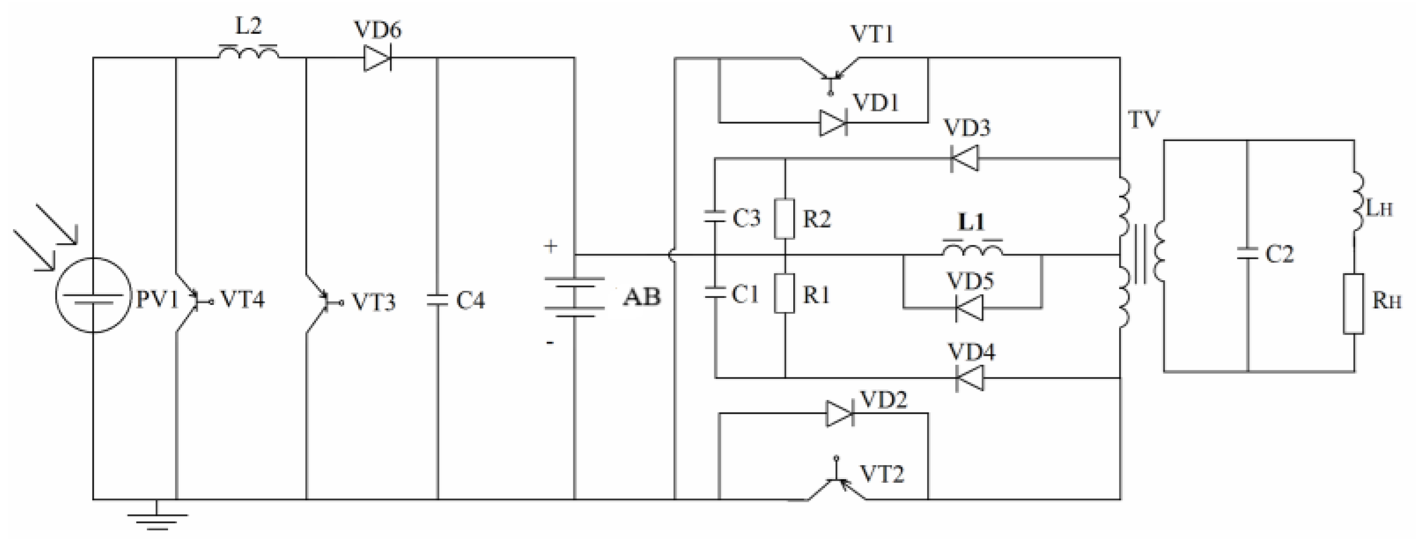
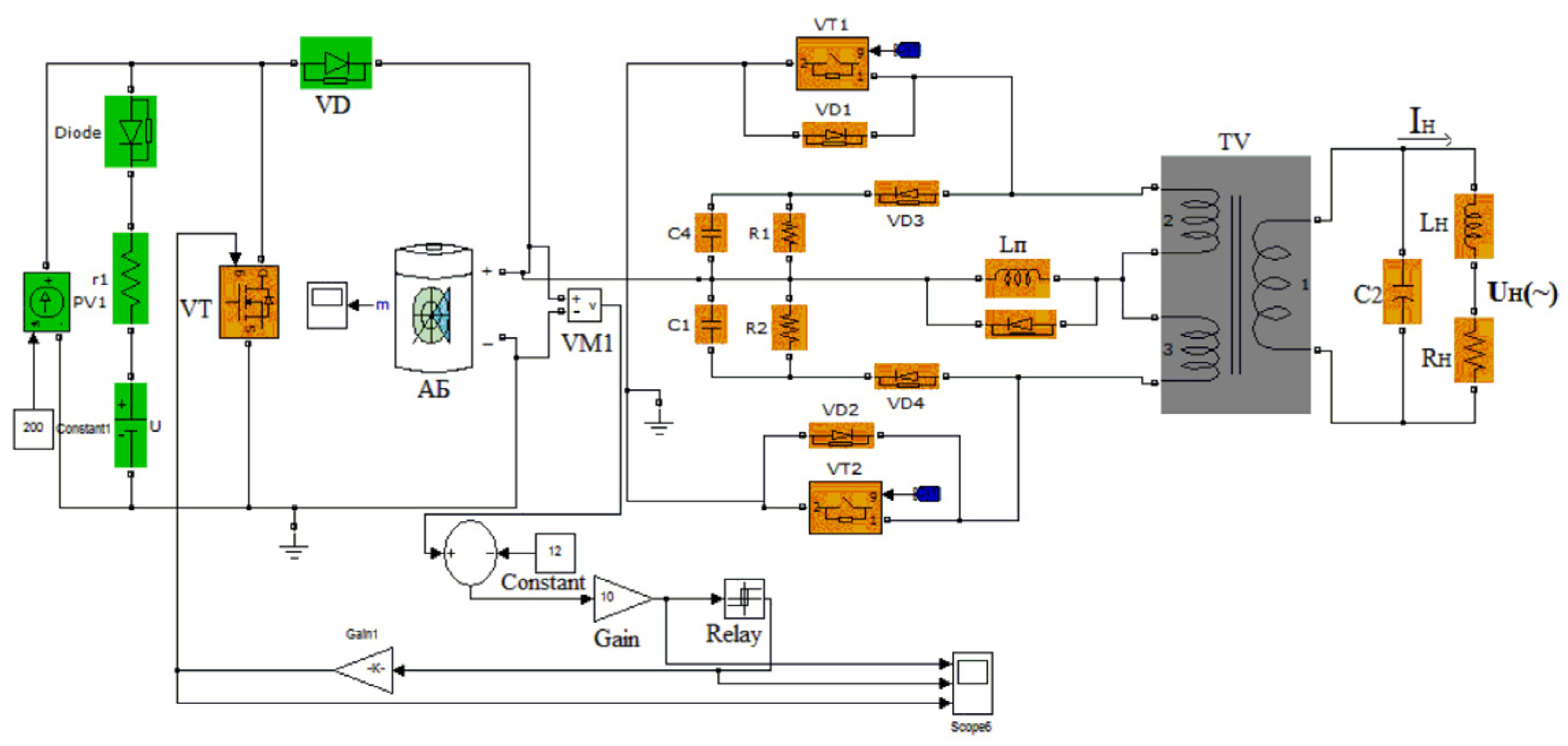
A system with solar-battery (SB) orientation is bulky and requires a complex automated electric drive that tracks the Sun. In our case, a fixed roof panel with a tilt angle β = 45° was suitable [7,34], to which the accumulator battery (AB) was connected in parallel. Users required a standard voltage of 220 V with a frequency of 50 Hz and used a stabilized sinusoidal voltage converter. In the dark hours of the day, the power supply of the converter (inverter) was provided by a battery that was charged during the day. The selection of the voltage of the panels was carried out by taking into account the safety of the power supply and the battery, which decreased with increasing voltage, and the reliability of the AB and SB. In high-voltage circuits (220 V), reliability decreases; a high-voltage AB has a large voltage between its elements and requires a complex balancing system to prevent damage; the best-developed design of ABs is automotive. A sealed lead–acid battery operates at a voltage of between 10 and 14 V. A hypothetical structure of an autonomous photovoltaic system is shown in Figure 1 and contains a current source, PV1, imitating a solar cell, a battery, and an inverter with a step-up transformer. The battery starts charging when the voltage of the solar battery increases to the minimum battery voltage level due to an increase in illumination, which is 10 ÷ 12 V.

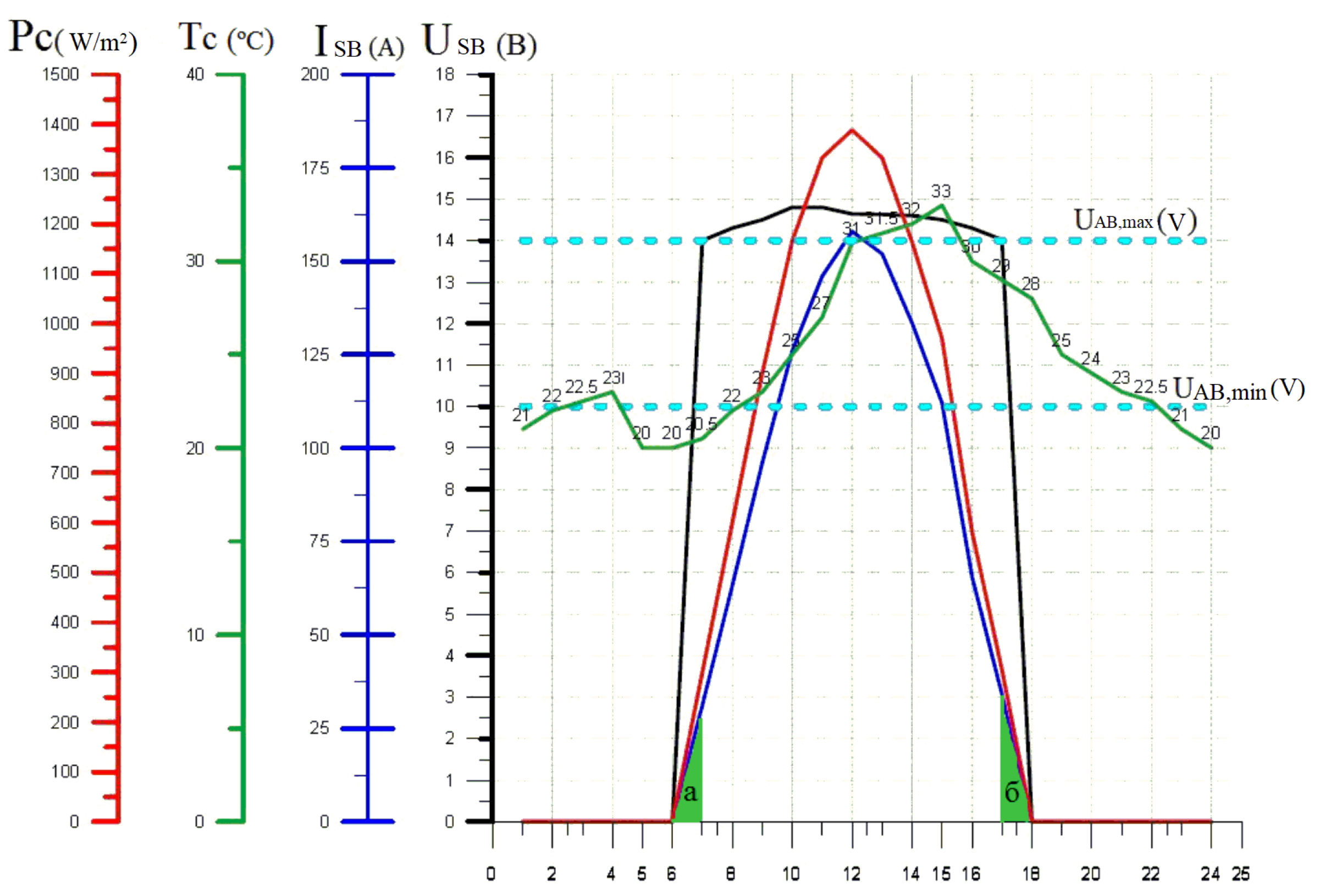
Figure 2 shows the possibilities for matching the energy characteristics of the elements of PV tubes, taking into account external conditions with the following typical characteristics: SB current ISB (A), SB voltage USB (V), change in ambient temperature T (°C), solar radiation power depending on the time of day PC (W/m²) [35,36,37]. It is clear that the energy deficit from the SB occurs from 6 to 7 in the morning and from 17 to 18 in the evening when USB < UAB, and energy losses are proportional to the area of triangles A and B.

We calculate the maximum charge theoretically separated from the $Q_{SB}$over the time of illumination as follows:

$$Q_{SB}=I_{SB}\ast t_c$$

(1)

We calculate the charge losses ∆Q when USB < UAB during the day. This happens twice every hour:

$$Q_m={\displaystyle \frac{I_{max∆}\ast t_{∆}}{2}}=Q_e,$$

(2)

where Q_m is the morning charge, Q_e is the evening charge, I_max∆ is the maximum charge of the SB one hour after sunrise, and t_∆ is the time when USB < UAB.

Let us calculate the total charge loss due to USB < UAB:

$${\sum }_{∆}{Q=∆Q}_m+{∆Q}_e,$$

(3)

Let us calculate the relative value of the charge loss without a converter:

$$\zeta ={\displaystyle \frac{\sum _{∆}Q}{Q_{SB}}}=2\%,$$

(4)

where ζ is part of the capacity loss.

Due to these 2% losses, there was no great need to increase the voltage. We proved that we could create a PV without a voltage converter between the power supply and the battery. It is relevant for southern regions. The converter on L2, VT3, and VD6 (Figure 1), which increases the voltage, had an efficiency of ≅ 0.8. Its inclusion allowed the use of energy to charge the battery from 6 to 7 in the morning and from 17 to 18 h (Figure 2). The extra energy, on the other hand, was equal to the losses in the boost converter L2, VT3, and VD6. This was because the areas of triangles A and B were equal, so we used a diode VD6 to connect SB and AB in parallel. The study aimed to determine the optimal voltage on AB and SB at fixed load parameters. We chose the PV structure with the simplest circuit for battery protection and control. Despite the optimal angle of inclination of the solar panel to the incoming solar radiation of β = 23°, which gives an annual solar energy income of 1977 kWh/m², the SB was installed on the roof with an angle of inclination β = 40°, which provided 1906 kWh/m² per year and provided protection from rain. We also demonstrated the feasibility of creating a PV without a voltage converter between SB and AB, which is crucial for tropical latitudes.

3. Forecasting Model Based on Interval Discrete Fuzzy Sets of the Second Type

Let $d\left(t\right)$($t$ = 0, 1, 2, …, m) be a time series based on the actual values of the forecast factor, and ∆d(t) (t = 1, 2, …, m) be a time series based on the increment values of this factor:

$$∆d\left(t\right)=d\left(t\right)-d\left(t-1\right)$$

(5)

The use of time series based on the values of factor increments allows for an increase in the accuracy of the developed forecasting model [38,39]. The universe X is:

$$X=D_{min}-D_1,D_{max}+D_2$$

(6)

where the series ∆d(t) is defined. Let D_min and D_max be the minimum and maximum values of the elements of the time series ∆d(t) (t = 1,2,…, m), respectively ($D_{min}=\underset{\mathit{t}=1,m}{\min }(∆d(t\left)\right)$. We can add up X of n intervals of lengths ($x_1$, $x_2$,…, $x_n$) using $D_1$ and $D_2$, which are real numbers [40,41]. Then, $\tilde{A}$, which is defined in the universe X, can be shown to be:

$$\tilde{A}=u_{\tilde{A}}(x_1)/x_1+u_{\tilde{A}}(x_2)/x_2+\dots +u_{\tilde{A}}(x_n)/x_n$$

(7)

where $u_{\tilde{A}}$($x_1$) are the lower and upper membership functions of the interval, x are discrete fuzzy sets of the second type, which are the normal ones for the interval and characterize the footprint of uncertainty (FOU), $u_{\tilde{A}}$($x_1$): X $\to$ [0, 1]; $u_{\tilde{A}}$($x_r$) (r = $\overline{1,n}$) is the value of the membership degree of the interval r of the universe X.

Figure 3 shows an example of the FOU uncertainty footprint for fuzzy sets of the second type.

The linguistic terms ${\tilde{A}}_r$ (r = $\overline{1,n}$) based on interval, discrete fuzzy sets of the second type can be represented as [42,43]:

$$\begin{gathered} {\tilde{A}}_1=1/x_1+\mathsf{\Lambda }/x_2+0/x_3+\dots +0/x_{n-1}+0/x_n, \\ {\tilde{A}}_2=\mathsf{\Lambda }/x_1+\mathsf{\Lambda }/x_2+0/x_3+\dots +0/x_4+0/x_n, \\ {\tilde{A}}_3=0/x_1+\mathsf{\Lambda }/x_2+1/x_3+\dots +\mathsf{\Lambda }/x_4+0/x_n, \\ \dots \dots \dots \dots \dots \dots \dots \dots \dots \dots \dots \dots \dots \dots \dots \dots \\ {\tilde{A}}_n=0/x_1+0/x_2+0/x_{n-2}+\dots +\mathsf{\Lambda }/x_{n-1}+1/x_n, \end{gathered}$$

(8)

where $\mathsf{\Lambda }={\alpha }_{lower},{\alpha }_{upper}; {{\alpha }_{lower} and \alpha }_{upper}$ are the lower and upper values of the membership function $u_A$($x_r$) for the interval $x_r$(r = $\overline{1,n}$).

The linguistic term $A_r$ (r = $\overline{1,n}$) corresponds to the uncertainty footprint FOU_r. The uncertainty footprint’s edges are set by the values of the lower and upper membership functions $u_{\tilde{A}}$($x_r$) and ${\overline{u}}_{\tilde{A}}$($x_r$) for the universe’s interval $x_r$ (r = $\overline{1,n}$). If the factor increment value belongs to the interval x₁, then the corresponding uncertainty footprint FOU₁ has the form:

$${\mathrm{FOU}}_1=0/{\tilde{A}}_1+\mathsf{\Lambda }/{\tilde{A}}_2(\mathsf{\Lambda }={\alpha }_{lower},{\alpha }_{upper})$$

(9)

If the factor increment value belongs to the interval $x_r$ (r = $\overline{2,n-1}$ ), then the corresponding uncertainty footprint FOU_r has the form:

$${FOU}_r=\mathsf{\Lambda }/{\tilde{A}}_{r-1}+1/{\tilde{A}}_r+\mathsf{\Lambda }/{\tilde{A}}_{r+1}(\mathsf{\Lambda }={\alpha }_{lower},{\alpha }_{upper})$$

(10)

If the factor increment value belongs to the interval x_n, then the corresponding fuzzy value FOU_n has the form:

$${FOU}_n=\mathsf{\Lambda }/{\tilde{A}}_{n-1}+1/{\tilde{A}}_n(\mathsf{\Lambda }={\alpha }_{lower},{\alpha }_{upper})$$

(11)

To construct the forecasting model based on FOU, the following steps are used:

• Let FOU_j and FOU_l be defined for the tth and (t + 1)th time readings of the time series. Then, a first-order fuzzy logical dependence can be made for these time readings: FOU_j → FOU_l.
• We can apply the same method to create a kth-order fuzzy logical dependence.
• We can define a fuzzy logical dependence group by combining the ones with the same left side into one.
• For instance, the formation would look like this:

$$\begin{gathered} {\mathrm{F}\mathrm{O}\mathrm{U}}_{j_k}{,\mathrm{F}\mathrm{O}\mathrm{U}}_{{j(}_{k-1)}},\dots , {\mathrm{F}\mathrm{O}\mathrm{U}}_{j_1}\to {\mathrm{F}\mathrm{O}\mathrm{U}}_{l_1}, \\ {\mathrm{F}\mathrm{O}\mathrm{U}}_{j_k}{,\mathrm{F}\mathrm{O}\mathrm{U}}_{{j(}_{k-1)}},\dots , {\mathrm{F}\mathrm{O}\mathrm{U}}_{j_1}\to {\mathrm{F}\mathrm{O}\mathrm{U}}_{l_2}, \\ \dots \dots \dots \dots \dots \dots \dots \dots \dots \dots \dots \dots \dots \dots \dots \dots \dots \dots \dots \\ {\mathrm{F}\mathrm{O}\mathrm{U}}_{j_k}{,\mathrm{F}\mathrm{O}\mathrm{U}}_{{j(}_{k-1)}},\dots , {\mathrm{F}\mathrm{O}\mathrm{U}}_{j_1}\to {\mathrm{F}\mathrm{O}\mathrm{U}}_{l_g}, \end{gathered}$$

(12)

Next, we combine them into groups.

$${\mathrm{F}\mathrm{O}\mathrm{U}}_{j_k}{,\mathrm{F}\mathrm{O}\mathrm{U}}_{{j(}_{k-1)}},\dots , {\mathrm{F}\mathrm{O}\mathrm{U}}_{j_1}\to {\mathrm{F}\mathrm{O}\mathrm{U}}_{l_1},{\mathrm{F}\mathrm{O}\mathrm{U}}_{l_2},\dots , {\mathrm{F}\mathrm{O}\mathrm{U}}_{l_g}$$

(13)

For the right parts $\mathsf{\Lambda }={\alpha }_{lower},{\alpha }_{upper}$, the lower and upper values of the membership function of the second-order fuzzy logical dependence are found in this way:

$$u_{\mathrm{F}\mathrm{O}\mathrm{U}}(x_r)=\max (u_{{FOU}_{l_1}}(x_r), u_{{FOU}_{l_2}}(x_r),\dots , u_{{FOU}_{l_g}}(x_r))(\mathrm{r}=\overline{1,n})$$

(14)

For the (t + 1)th time reading, the dependence found is made up of the first type of discrete fuzzy sets that are linked to the lower and upper values of the membership function for the FOU model. If no repeating elements exist, we employ forecasting. FOUs in the right parts are required to account for repetitions. It is necessary to modify the formula to calculate the defuzzified value of the coefficient increments y(t + 1) for the (t + 1)th time reading, adding coefficients corresponding to the multiplicity of uncertainty. To find the expected value for the (t + 1)th time sample, we add the known value of the element d(t) for the tenth time sample to the centroid value for the factory increase for the (t + 1)th time reading.

4. Calculation of the Centroid of an Interval Discrete Fuzzy Set of the Second Type

We use the type-reduction operation [40,41,42] to find the value of the centroid y(t + 1) for the (t + 1)th time sample. During this operation, two discrete fuzzy sets of the first type (DFST1) are defined and placed within the FOU. A second type of discrete fuzzy set with minimum and maximum centroids in $\tilde{A}$ is also defined [43,44].

We calculate the average-weighted centroid of DFST1 as follows:

$$y\left(t+1\right)={\sum }_{r=1}{w}_r\left(t+1\right)*{\displaystyle \frac{{\chi }_r}{\sum _{r=1}{w}_r\left(t+1\right)}},$$

(15)

where ${\chi }_r$ is the midpoint of the rth interval, w_r(t + 1) is the degree of membership for the (t + 1) period. Moreover, in expressions (13) and (14), instead of the FOU, DFST1 appears. By putting the DFST1 into the FOU, we can find the centroid $C_{\tilde{A}}$ of a second-type interval discrete fuzzy set:

$$C_{\tilde{A}}={\int }_{z_1ϵZ_1}^z\dots {\int }_{z_nϵZ_n}^z\dots ,{\int }_{w_1ϵW_1}^w\dots {\int }_{w_nϵW_n}^{w}1/({\sum }_{r=1}^n{w}_r\left(t+1\right)\ast z_r/{\sum }_{r=1}^n{w}_r\left(t+1\right))=\left[y_{left},y_{right}\right],$$

(16)

where $Z_r$ ($r=\overline{1, n) }$e DFST2 with center r and degree of spread spread_r ≥ 0, W_r (r = (1, n)) e DFST2 with center hr and length Δr ≥ 0), zr is the midpoint of the rth interval, [y_left, y_right] are the left and right endpoints of the DFST2.

As a result of applying Formula (16), an interval [y_left, y_right] is determined based on the values of the boundaries of which the value y(t + 1) for the (t + 1)th reading is calculated:

$$y(\mathrm{t}+1)={\displaystyle \frac{y_{left},y_{right}}{2}}$$

(17)

Thus, to calculate the centroid $C_{\tilde{A}}$, two endpoints of the interval must be found y_left and y_right, defining its boundaries. The value of the centroid can be calculated using the well-known iterative Karnik–Mendel algorithm [40,41,42], as well as some other special algorithms that significantly reduce computational costs. The basic FOU prediction model uses the mean relative error as a single quality assessment criterion. The forecast error (AFER—average predicting error rate) must be minimized:

$$AFER={\displaystyle \frac{\sum _{t=k+2}^m\left|\right(f\left(t\right)-d\left(t\right))/D(t)}{m}}\ast 100\%,$$

(18)

where f(t) and d(t) are the forecast and actual values for the period, m is the value of the time series, and k is the order of the forecasting model.

5. Genetic Algorithm for Searching for Optimal Parameter - Values: FOU Prediction Model

When developing a FOU (footprint of uncertainty) prediction model, the task is to find optimal values for the prediction model parameters with maximum accuracy. These are real numbers D₁ and D₂ used in adjusting the universe’s boundaries, the number of separation intervals n of X, the order k of the prediction model, and the degrees of membership αlower and αupper. Using a genetic algorithm reduces the time required to search for optimal values of the FOU parameters. The model parameters should be selected as follows: the right-hand sides of all fuzzy logical dependencies’ (FLDs) groups at t ≤ m. For the FOU prediction model, the chromosome in GA was defined in the following interval [45,46]:

S = (D_1, D_2, n, k, α_lower, α_upper),

(19)

For each element of the chromosome, a range of variation was set for D1—[0, dl₁], for D₂—[0, dl₂], for n—[2; n_max], for α_lower and α_upper—[0; 1], for k—[2; k_max], where dl₁ and dl₂ are positive numbers equal to d_li = D_max − D_min, i = 1, 2, n_max is a natural number n_max < m − 1, m is a number that takes into account time, and k_max is a natural number k_max < m − 1. In a GA, it is important to check if it is possible to make a group of fuzzy logical dependencies (GFLD) with non-empty right sides both when creating the initial population of chromosomes and when producing offspring chromosomes for each new set (D₁, D₂, n, k, α_lower, α_upper). After completing this step, we calculated the correspondence function using the following formula:

$$AFER={\displaystyle \frac{\sum _{t=k+2}^m(f\left(t\right)-d\left(t\right))/D\left(t\right)}{m}}\ast 100\%,$$

(20)

where AFER is the average forecasting error rate, f(t) and d(t) are the predicted and actual values for the tth time count, m is the number of time counts, k is the order of the forecasting model, and the set (D₁, D₂, n, k, α_lower, α_upper) was added to the quality of the chromosomes in the population. Otherwise, (D₁, D₂, n, k, α_lower, α_upper) was rejected as “non-viable”. Simultaneously, we must consider the “non-viability” of the set in some manner when calculating the matching functions [38,39,40]. Additionally, when applying GA, we must ensure that the following condition is satisfied: α_lower and α_upper, i.e., the numbers determine the “lower” and “upper” values, respectively. In addition, each of the sets (D₁, D₂, n, k, α_lower) and (D₁, D₂, n, k, α_upper) was checked for “viability”. If at least one of them was recognized as “non-viable”, then the corresponding chromosome (D₁, D₂, n, k, α_lower, α_upper) was also recognized as non-viable. Then, we used the Karnik–Mendel algorithm for each chromosome. This algorithm figures out the fitness function value using Formula (2). This value indicates the average relative error in predicting AFER. When implementing a GA, it is crucial to focus on creating an initial population that only includes “viable” chromosomes. In our case, implementing the crossover and mutation operations was more efficient. In the current GA generation, we recognized the chromosome that provided the minimum value of the fitness function based on Formula (2) as the best. We knew that chromosome s = (D₁, D₂, n, k, α_lower, α_upper)) was not viable if the average relative prediction error (20) for (D₁, D₂, n, k, α_lower) and (D₁, D₂, n, k, α_upper) was less than the values Fit_lower and Fit_upper. This meant that the function Fit(s) was set to 100. Otherwise, s = (D₁, D₂, n, k, α_lower, α_upper) was recognized as viable, and the value of its fitness function Fit(s) was assumed to be equal to AFER (20). In this regard, Fit(s) was defined in the GA as follows:

$$\mathrm{Fit}(\mathrm{s})=\left\{\begin{array}{c}AFER, if AFER<{Fit}_{lower} and AFER<{Fit}_{upper}\\ 100, else \end{array}\right.$$

(21)

We used a two-stage analysis of time series variability with the FOU forecasting model. You could use the model to guess the future values of different parts of the BP that described a certain process, as well as the values of different characteristics, like the Hurst exponent [45,46]. As is known, the preliminary calculation of such characteristics allowed us to conclude about the predictability of the initial time series itself, hence for forecasting using certain forecasting models. The quality of the basic FOU forecasting model was improved by introducing an additional quality assessment criterion, the trend, which had to be minimized [47]. The trend had the following form [47,48]:

$$\mathrm{T}\mathrm{e}\mathrm{n}\mathrm{d}\mathrm{e}\mathrm{n}\mathrm{c}\mathrm{y}={\displaystyle \frac{\mathrm{h}}{m-k-1}}$$

(22)

where h is the number of negative products of (f(t − 1) − f (t) ∗ (d(t − 1) − d(t)), when t = $\overline{k ,2 m}$, f (t) and d(t) are the predicted and actual values of the BP elements for period t, m is the number of time counts; k is the order of the forecasting model; m—k − 1 is the total number of products (f(t − 1) − f (t) ∗ (d(t − 1) − d(t)).

The Hurst indicator showed the relationship between the strength of the trend and the noise level (i.e., the random component). It was calculated using the results of the time series analysis and was an estimate of the ratio between the amount of variation in the first m values of the time series and the standard deviation S. To calculate the values of the TS elements, representing the values of the Hurst exponent, we used the following algorithm [49,50].

• We set the current length τ of the BP x_i (i = $\overline{1,\tau }$) equal to 3, $\tau$ = 3.
• We calculated the mean $\overline{x_{\tau }}$ and standard deviation S_τ for values of x_i (i = $\overline{1,\tau }$) elements of the TS with the current length τ.
• We calculated for each value x_i (i = $\overline{1,\tau }$) the deviation from the mean $\overline{x_{\tau }}$: Δ_i = x_i − $\overline{x_{\tau }}$ (i = $\overline{1,\tau }$). We found the sum (sum)_t of the differences between the values xi (i = ($\overline{1,\tau }$)) of TS elements of the current length and the mean value x_τ for each time t, (t = $\overline{1,\tau }$):

$${sum}_t={\sum }_{i=1}^t{∆}_i={\sum }_{i=1}^t\mathrm{x}\mathrm{i}\overline{x_{\tau }}$$

(23)

4.

We calculated the minimum and maximum values of the average sums of the TS with the current length $\tau$:

$$\begin{gathered} {minSum}_{\tau }=\underset{\mathrm{t}=\overline{1,\tau }}{\min }\left({sum}_t\right) \\ {maxSum}_{\tau }=\underset{\mathrm{t}=\overline{1,\tau }}{\max }\left({sum}_t\right) \end{gathered}$$

(24)

We calculated the range $R_{\tau }={maxSum}_{\tau }-$ ${minSum}_{\tau },$normalized to the value S_τ with the range RS_τ = R_τ/S_τ for the values of the Hurst exponent $H_{\tau }=\ln \left(\mathrm{R}\mathrm{S}\mathsf{\tau }\right)$/$\ln \left({\displaystyle \frac{\tau }{2}}\right).$

5.

We increased the current length of the TS by 1.

6.

If the current length of the TS was less than or equal to the length of the analyzed TS, we proceeded to step 2. Otherwise, we proceeded to step 7.

7.

We calculated the average values of the Hurst exponent for all lengths:

$${\overline{H}}_m={\sum }_{\tau =3}^m{H}_{\tau }/(n-2)$$

(25)

8.

End of the algorithm.

It should be noted that the longer the BP length, the more accurate the estimates of the Hurst exponent will be [51,52]. In the FOU model, the value of the Hurst exponent first helps us obtain a rough idea of how quickly we can perform the forecasting process one step ahead of time. It also helps us obtain a rough idea of the “range” of the parameters of the “uncertainty footprint of FOU”. Implementing GA directly considers the specifics of the applied problem, which involves searching for optimal parameter values. First, we must determine the structure of a chromosome and its encoding method. Next, we determine the method for selecting chromosome parents, as well as the procedures for crossover and mutation. Finally, we choose a favorable correspondence function, which we need to minimize when we apply GA [53].

The chromosome providing the minimum value of the fitness function (21) is recognized as the best in the current generation of the GA. In the context of the task of developing a model for predicting FOU for the selection of parents in GA, the principle of probabilistic selection was used: the smaller the value of the fitness function of chromosome sl (l = ($\overline{1, p}$) in the current population, the greater the probability p_l that chromosome sl will act as a parental chromosome in forming offspring chromosomes for a new population.

When performing the crossover operation in GA, the parent chromosome was selected according to the following algorithm.

1. Sort by increasing probability $p_1$ (l = $\overline{1, p}$);

2. Generate a random (uniformly distributed) number z from the interval [0, 1]: z = random([1, 0]);

3. Select chromosome l as the parent chromosome if the random number z falls into the lth interval [$p_{l-1};$ $p_1$ (l = $\overline{0, p}$); $p_0$ = 0]. To determine the two parent chromosomes, steps 2 and 3 are repeated twice. For the crossover operation, the crossover coefficient Rc is fixed. A random number z_c random([1, 0]), c = is generated when attempting to cross two parent chromosomes. If R_c > z_c, then the intersection point is chosen c $r_m$ ($r_m$ ∈ {1, 2, 3, 4, 5) and the intersection is performed with two parental chromosomes and the formation of two offspring chromosomes. For the mutation operation, the crossover coefficient Rm is fixed.

When applying a GA, a single-point crossover of the parental chromosomes is performed and no more than one element (gene) in the parental chromosome undergoes mutation. The GA for a predictive model of FOU can be described by the following sequence of steps (Figure 4):

• Create an initial population of chromosomes of size P from randomly selected viable chromosomes of the type s = (D1, D2, n, k, α_lower, α_upper) taking into account the calculation of the values of the fit function and the removal of non-viable candidates from consideration.
• Sort the chromosomes of the initial population in increasing order of the values of the fit function.
• Perform crossover and mutation operations on the current population of chromosomes.
• Calculate the values of the fit function for each chromosome of the offspring.
• Form an expanded population of chromosomes of size P + R_c*P, from the current population of size P and offspring chromosomes.
• Go to step 3 when g ≤ G, increasing the current number of generations g by 1 (G and g are the maximum and current number of generations of the GA, respectively). Go to step 7 when g > G.
• Choose the best chromosome, i.e., the one with the minimal fit value.

First, the structure of chromosomes and the method of their encoding must be determined. The technique for selecting parental chromosomes must also be determined, and then the possibilities for crossover and mutation operations must be defined. We chose an adequate fit function, which should be minimized (maximized) when applying the GA. This function ultimately determines the direction of development of the chromosome population to select the best chromosome. In the context of the task of developing a model for predicting the FOU structure, the chromosomes in the GA were defined as (D₁, D₂, n, k, α_lower) and (D₁, D₂, n, k, α_upper), where D₁ and D₂ are the correction numbers of the boundaries of the universe X, on which the TS is defined, n is the number of intervals of division of the universe X, k is the order of the prediction model, and α_lower and α_upper are values of the degrees of membership according to the Fit(s) function.

In our case, the encoding of all chromosome elements was carried out using real numbers. The condition α_upper ≥ α_lower was satisfied by the proposals specified in Section 3. Two values of the Fit(s) functions, Fit_lower and _Fitupper, were calculated (for the “lower” and “upper” values of the membership function of the fuzzy sets of the second type). Suppose the values of the Fit(s) functions are equal to 100. In that case, the chromosome corresponding to them is considered “non-viable”, and the value of its fitness function Fit(s) is taken to be equal to 100. Otherwise, chromosome s = (D₁, D₂, n, k, α_lower, α_upper) is considered “viable”, and the average relative prediction error AFER is calculated using the iterative Karnik–Mendel algorithm.

If the value of the average relative prediction error (20) for a chromosome s is less than the values of the Fit_lower and Fit_upper matching functions for sets (D₁, D₂, n, k, α_lower) and (D₁, D₂, n, k, α_upper), respectively, then such a chromosome is recognized as “viable”, and the value of its matching function Fit(s) is equal to AFER. Otherwise, the Fit(s) value of this chromosome is 100.

6. Results

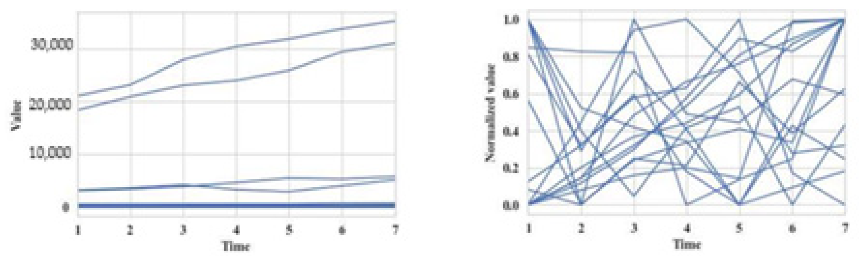
We used a set of 60 synthesized TSs as model data, each containing numerical values for seven periods. Such a small TS length was chosen because the result was the TS length corresponding to the real analyzed energy consumption in residential buildings in cold weather. The first example’s time series (TS) was part of six clusters formed by transforming six base patterns (TSs) using periodic functions like sine and cosine. We warped the original model set of TSs to assign it to a new cluster. A visualization of the initial set of TSs of six clusters is presented in Figure 5a, where time is a countdown of time and value is the value of the TS element. The graphs of different clusters are indicated in various colors, while the graphs of TSs forming the initial clusters are grouped and create a “thick” line. The distorted graph was obtained based on the values of the elements of one of the TS that belonged to the cluster whose TSs were located at the bottom of the group by changing their values starting from the third time point. The new TSs should have formed a new cluster. The algorithm confirmed this fact as seen in further detail in the following.

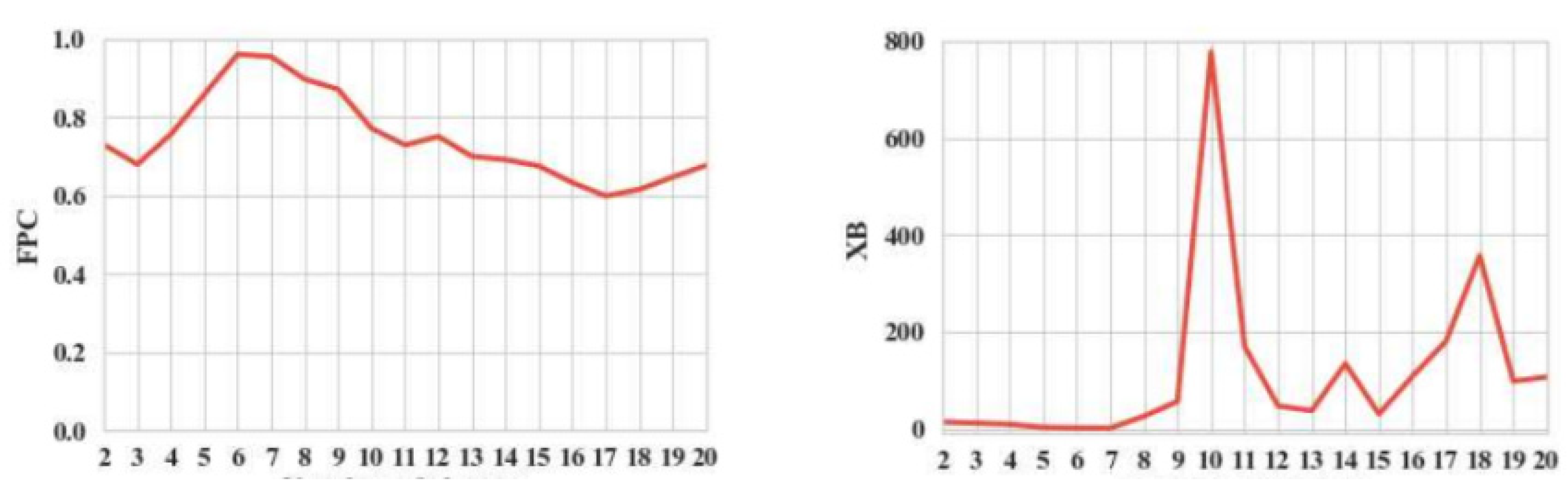
Figure 5b shows the normalized initial set of TSs and the normalized distorted TSs. Using the algorithm on a normalized initial set of time frames with t = (3.7) allowed us to find six groups, with time frame lengths of three, five, six, and seven. The best number of six clusters was determined by minimizing the XB index.

The XB index made it possible to determine that the optimal number of clusters was five, with the number of time samples equal to four. Poor separability with a sample count equal to four can explain these clustering results.

It is important to note that for TSs with lengths three and four, both clustering quality indicators (XB index) agreed on the best number of clusters. Using the algorithm on a normalized skewed set of time frames helped us find six clusters when there were three time samples and five clusters when there were four time samples. Applying the algorithm on a normalized skewed set of time frames made it possible to identify six clusters with the number of time samples equal to three and five clusters with several time counts equal to four. For TSs of length three and four, both clustering quality indicators (XB index) gave a consistent solution for the optimal number of clusters.

With several time samples equal to five, six, and seven, the XB index determined that seven was the optimal number of clusters.

The distorted graph was obtained based on the values of the elements of one of the TSs that belonged to the cluster whose TSs were located at the bottom of the group by changing their values, starting from the third time point.

The new TSs should have formed a new cluster. We further confirmed this fact using the algorithm. Figure 5b shows the normalized initial set of TS and the normalized distorted TS. Implementing the algorithm on the normalized initial set of time frames with the number of time samples t = (3.7) made it possible to identify six clusters with time frame lengths equal to five, six, and seven.

The use of the Hurst index (XB) at four time points allowed us to determine that the optimal number of clusters was five (

Table 1. Determining the optimal number of clusters with the XB index and fuzzy algorithm.

Clustering Quality Indicator				Number Clusters	Number of Time Reports
					3	4	5	6	7
XB	5	316,732	2882	2373	1965		1754
	6	3319	47,751	1037	0.611		0.551
	7	1778	21,735	0.906	0.518		0.469
Fuzzy algorithm	5	0.849	0.893	0.858	0.875		0.874
	6	0.928	0.846	0.961	0.969		0.97
	7	0.897	0.874	0.955	0.966		0.967

and Figure 6).

Testing of the proposed algorithms with a two-stage method of TS variability was carried out based on a real group of indicators when studying the location and operation of small photovoltaic installations for household consumers in sparsely populated areas in southeastern Bulgaria for the period from 2021 to 2024. Among them, there were multiple indicators presented by TSs and grouped into the following categories: according to the electricity consumption in homes; according to the inclination of the solar panels, at the optimal inclination angle of the solar panel of β = 23°, which gave maximum annual solar energy; depending on the meteorological conditions since from March to September, solar radiation is higher compared to that from October to February and, then decreases by 19%, and the probability of precipitation is increased; according to the chosen design and voltage of the autonomous photovoltaic installation; according to the area and capacity of the solar cells; according to the influence of ambient temperature on the performance of the solar cells; according to the energy balance of the photovoltaic installations; and according to the differences in the inverter schemes.

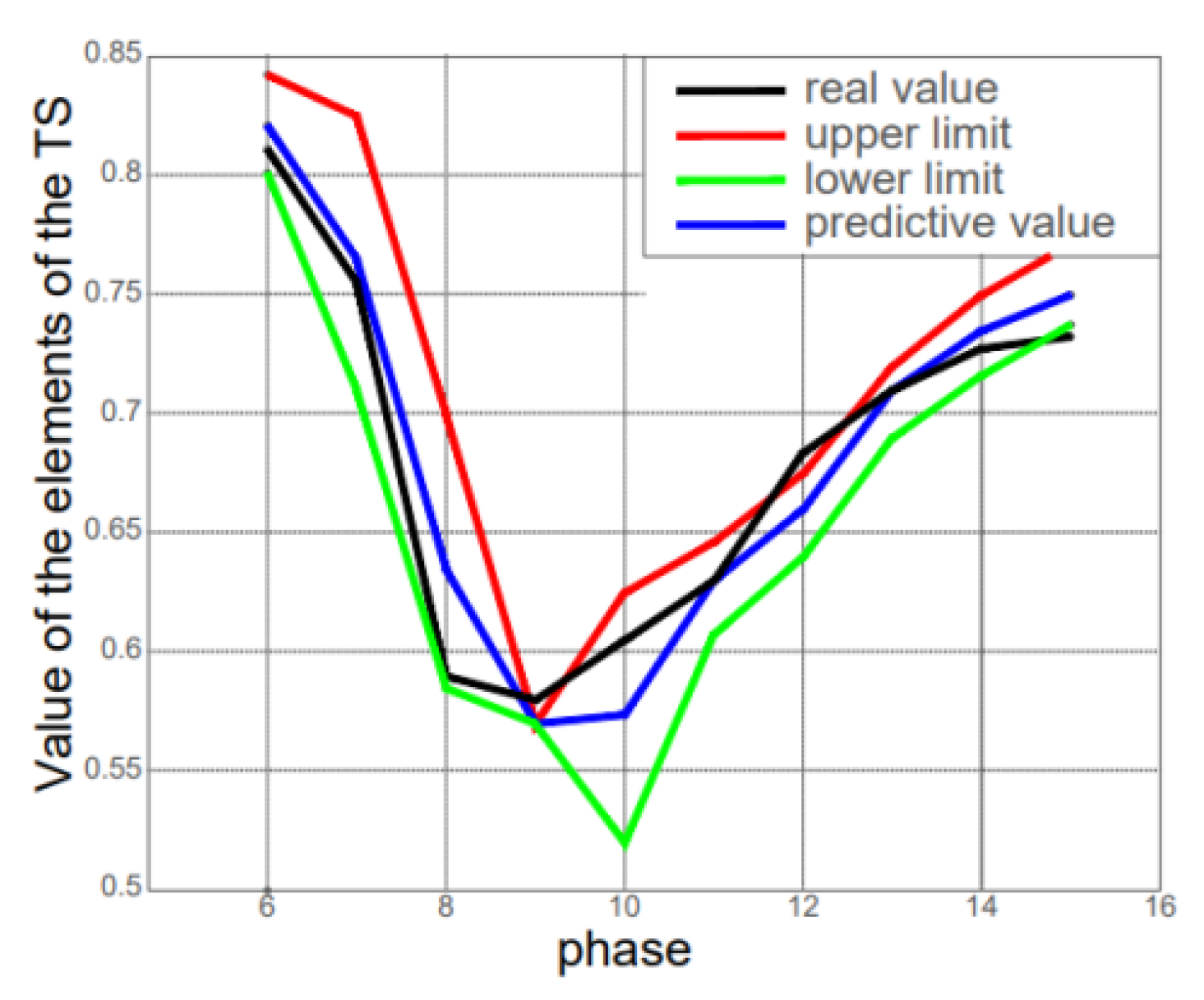
For each of the considered TSs, models were created containing Hurst exponent values and indicators that corresponded to the original TSs. For TSs T1 and T2, the FOU prediction model was determined as optimal with the following parameter values: D₁ = −0.115; D₂ = 0.123; number of separation intervals n = 3; model order k = 7; α_lower = 0.0094 and α_upper = 0.094. At the same time, the values of the quality criteria were as follows: AFER = 0.854%; Trend = 0.167 (Figure 7, Figure 8, Figure 9, Figure 10 and Figure 11).

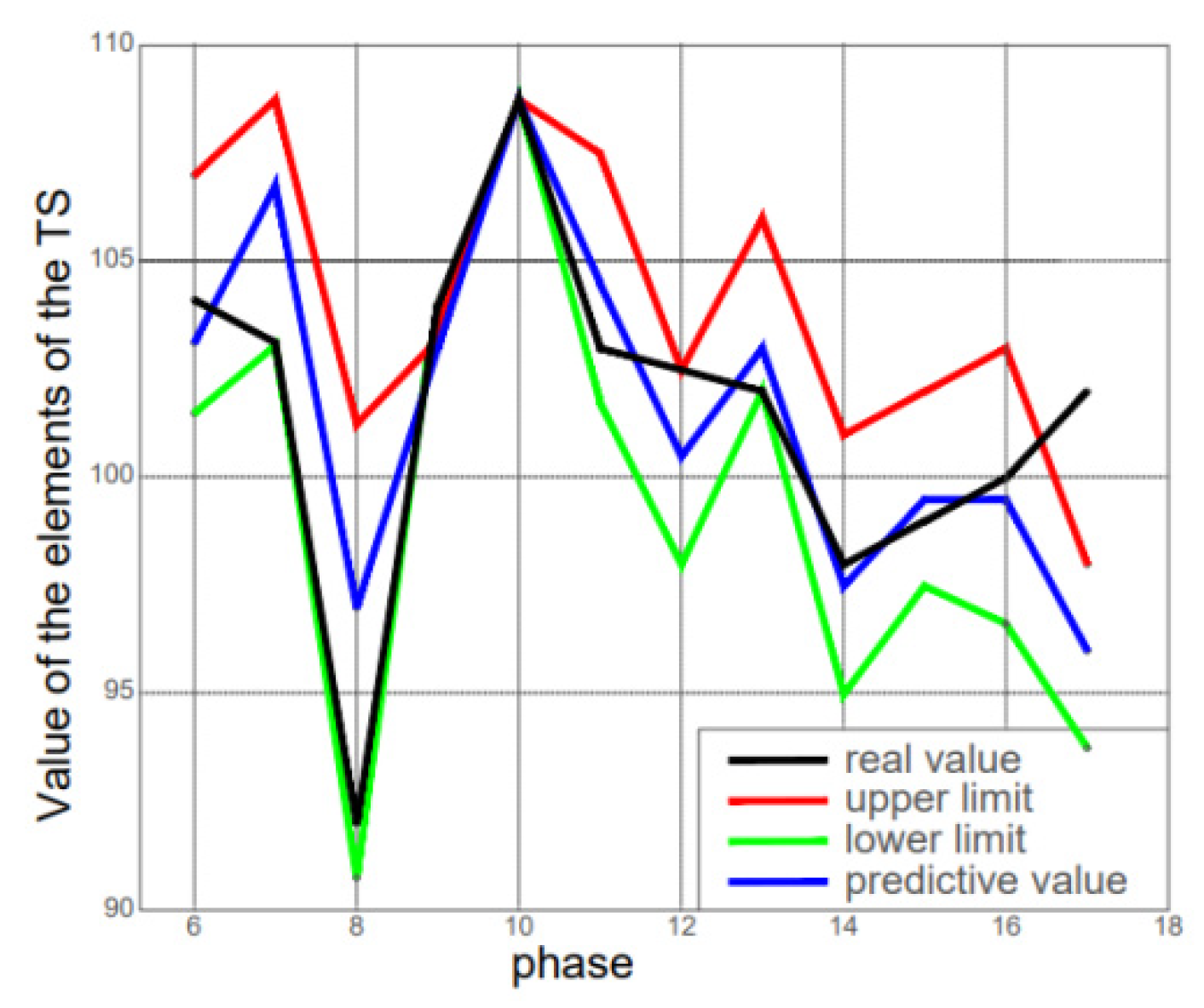
In the following, we present the results of developing the FOU model for the TSs, which contained 18 elements and characterized specific indicators. Figure 8 shows the index of the physical volume depending on the meteorological conditions as % k from the previous year (original VR). Figure 9 shows the index of the physical volume according to the chosen design and voltage of the autonomous photovoltaic installation.

Developing the FOU model for TSs yielded results that characterized the Hurst index for specific indicators. Figure 10 shows the nominal values according to the energy balance of photovoltaic installations for one year, and Figure 11 demonstrates the influence of ambient temperature on the performance of solar cells.

• Parameters: $D_1$ = −0.115, n = 3, ${\alpha }_{lower}$ = 0.0094, ${\alpha }_{upper}=$0.094,
• $D_2$ = 0.123, k = 7.
• Indicators: AFER = 0.854; Tendency = 0.167.

Inferences: Examining the basic prediction model without accounting for uncertainty realized forecasting one step further. We conclude that the parameters of the prediction model should be chosen so that the right parts of all groups of fuzzy logical dependencies are non-empty. It is evident that to assess the quality of the prediction model, it is advisable to use the average relative prediction error specified in (20). The developed GA, which searched for optimal values of the prediction model’s parameters and ensured the minimization of the compliance function based on the average relative prediction error, had an acceptable time cost. It was shown that the compliance function allowed the exclusion of unviable chromosomes that could not reproduce (21), which meant that the groups of fuzzy logical dependencies had at least one empty right part from the current population of chromosomes.

7. Discussion

After testing and analyzing the parameters in the study of how small photovoltaic systems for home use work, we used Simulink to create a model of the structure of an autonomic photovoltaic system.

Table 2. The parameter ranges of the PV models.

Parameter	Single Diode/Double Diode		PV Module MC4		PV Module SFR		PV Module EVO2
	LB	UB	LB	UB	LB	UB	LB	UB
Iph (A)	0	1	0	2	0	2	0	2
Isd, Isd1, Isd2, (μA)	0	1	0	50	0	50	0	50
RS (Ω)	0	0.5	0	2	0	0.5	0	0.5
Rsh (Ω)	0	100	0	2000	0	1000	0	1500
n, n1, n2	1	2	1	50	1	50	1	50

shows the parameter ranges of the PV models.

Considering the elements’ analysis, the solar battery was located on the roof and was permanently oriented to the south with a selected tilt angle of β = 40°. The study aimed to determine the optimal voltage of the battery and solar battery and the type of voltage converter at fixed load parameters. The analysis showed an AB and SB with a voltage between 14 V and 220 V and an inverter at an alternating voltage of 220 V with a frequency of 50 Hz and a sinusoidal shape with a distortion of less than 10% (Figure 12).

PV1 connected to the battery for charging. Including a controller in the battery circuit (VM1) was necessary to prevent overcharging the battery. When the solar battery was charged to the desired maximum voltage, an overcharging warning circuit parallel to the solar panel charged the transistor VT to absorb the excess solar energy of the panels. The battery was protected from overcharging by a relay regulator containing a reference voltage sensor constant, a device for comparing the voltage with a constant block, a gain regulator for amplifying the error, and a relay block that controlled VT. When the charging voltage reached 14 V, the battery short-circuited the VT switch. We tested the inverter using a rectangular and regulated output voltage at 50 Hz. A parallel resonant LC circuit connected to the inverter via a transformer provided the sinusoidal voltage wave on the load. Inductance LP smoothed the current consumed by the inverter. Inductance LH was an active-inductive load with cos φ = 0.8 and a parallel-connected transformer TV with a capacitor C2. They formed a parallel resonant circuit. A capacitor, C2, connected to the load, giving it a sinusoidal shape. Based on this information, we studied several options for inverter circuits. We selected a circuit based on three criteria: reliability, no transistor overvoltage, distortion less than 10%.

We chose a photovoltaic structure with the simplest circuit for protection and control of the battery without a boost converter between the power supply and the battery. Despite the optimal angle of inclination of the solar panel relative to the incoming solar radiation, β = 23°, which gave an annual income from solar energy of 1876 kWh/m² per year, the SB was installed on the roof with an angle of inclination β = 40°, which provided 1806 kWh/m² per year and provided protection from precipitation. The possibility of creating a photovoltaic without a voltage converter between the SB and AB is relevant for tropical latitudes. The analysis led to the selection of the AB from seven maintenance-free types with a maximum energy density of 180 W/kg. We selected the method to protect the battery from overvoltage.

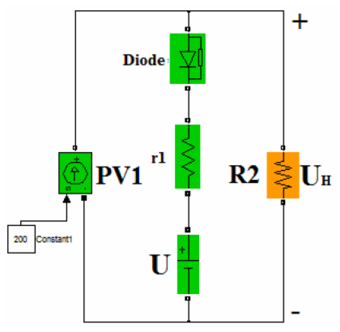
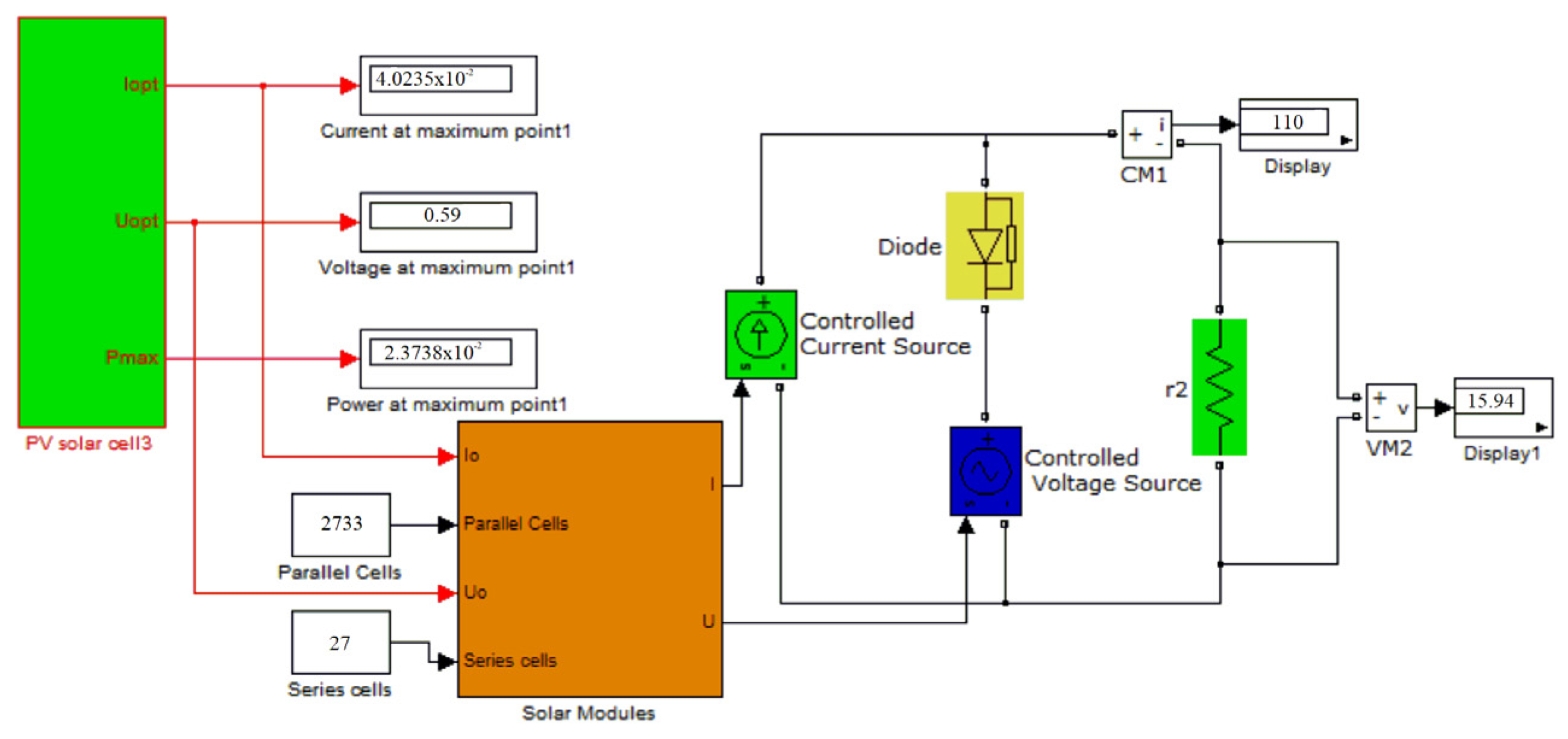
We modeled the solar battery in Simulink, taking into account changes in solar radiation and ambient temperature. The peculiarity of the model was the volt–ampere characteristic of the SB. It passed through three points: open-circuit voltage, short-circuit current, and maximum power point. The SB model consisted of a current source PV1 (Figure 13), equal to the short-circuit current of the SB, a voltage source U, a resistor r, and a diode VD, whose values were calculated from the following equations. For the SB model with a volt–ampere characteristic close to the real one, we calculated the value of the parameters (Figure 14) as follows:

Idling:

$$U_{sb}=U+U_{VD}+I_{sb}$$

(26)

At maximum power:

$${U_{max}=(I}_{sb}-I_{max})\ast r+U_{VD}+U$$

(27)

From Equations (26) and (27), we calculated the unknown parameters U and r:

$$U=U_{sb}{\displaystyle \frac{(K_i+K_n-1)}{K_i}}-U_{VD}$$

(28)

$$r={\displaystyle \frac{U_{sb}}{I_{sb}}}\ast {\displaystyle \frac{(1-K_n)}{K_i}}$$

(29)

The results of the SE simulations of the solar module is shown in Figure 15. Other parameters, such as the fill factor ζ (F), efficiency, and temperature coefficients of voltage and current, can be seen in the MatLab workspace in this form.

When working on the optimization problem of the FOU forecasting model, we needed to consider how to calculate the compliance function, which involved checking if it can be created with non-empty right sides. When looking at the basic forecasting model without repeating elements, we found that the parameters of the forecasting model needed to be selected so that the right sides of all groups of fuzzy logical dependencies, based on a fuzzy logical dependency, were not empty. Another limitation was the problem of controlling the “lower” and “upper” values of membership functions of an interval discrete fuzzy set of the second type. It was shown in the forecasting model that the uncertainty of the choice of values of the degree of membership for the TC element, corresponding to time accounting and belonging to some interval, could be controlled. Despite these limitations, this paper revealed the trend and problems in the estimation of photovoltaic parameters, which will help future researchers further improve the efficiency of parameter estimation. The application of the developed forecasting model gave results similar to classical models but typically increased forecasting accuracy by one step and shortened the processing time.

8. Conclusions

An algorithm for predicting FOU was developed, which differed from classical models because it did not impose strict requirements for the good separability of clusters on a group of time series. It allowed us to analyze the behavior of groups of indicators for the energy-efficiency evaluation of small PV systems for domestic consumers. It facilitated the identification of structural transformations at early stages. The results of the forecasting and analysis, presented in a concise time series using the developed algorithm, can serve as a foundation for enhancing the adequacy and validity of decisions made based on the information received within an acceptable time frame.

We used Simulink to model the structure of an independent photovoltaic system and tested and analyzed it. We also modeled a solar battery, considering changes in solar radiation and ambient temperature.

We introduced extended tabular characteristics of the SB, enabling reasonable selection. We experimentally measured the SB’s actual volt–ampere characteristics. The structure of the photovoltaic system directly connected the SB and AB, eliminating the need for an additional choke in the inverter circuit. In future research, we could add a comparative analysis of the FOU forecasting model and traditional algorithms. We could also consider the compliance function by developing the author’s version of a multi-criteria GA for identifying the Pareto front solutions.