1. Introduction
Economic development necessitates and promotes the growth of cargo transportation. In practice, there are many large-sized products and packages, such as steel coils, prefabricated building components, and electromechanical devices. Due to constraints related to loading and unloading time, transportation space, and transportation costs, these packages often cannot be secured using fastener measures and are referred to as freestanding packages. During transportation, freestanding packages may exhibit various dynamic responses, including rocking, sliding, and jumping, in reaction to vehicle acceleration. Among these responses, rocking motion is particularly critical for transportation safety. If the rocking angle of a package exceeds a critical threshold, it may overturn, potentially leading to severe traffic accidents. Therefore, it is essential to determine the dynamic response states, analyze the rocking behavior, and assess the overturning risks of freestanding packages.
The package is simplified and modeled as a rigid block, and the safety requirements for package transportation have prompted extensive research into determining motion states and analyzing the rocking motion of rigid blocks on moving bases. The possible motion states of a rigid block on a moving base have been analytically determined in [
1]. Among these states, rocking and overturning are particularly detrimental to transportation safety. Considering the resurrection phenomenon and the weaving behavior of the rocking Incremental Dynamic Analysis (IDA) curve, the IDA method [
2,
3] was refined and applied to evaluate the rocking behavior and overturning probability of freestanding rigid blocks [
4]. In [
5], numerical analysis was conducted to assess the statistical distribution and overturning probability of freestanding rigid blocks, revealing that the peak ground velocity is the most effective ground motion intensity measure for predicting rocking behavior. Similarly, in [
6], various ground motion intensity measures were tested by fitting power-law models to evaluate their effectiveness in predicting rocking response characteristics and overturning risks. Kazantzi et al. [
7] proposed a set of
I-
θ-
p equations derived through nonlinear regression to predict rocking response characteristics, which can be used to assess the overturning risks of freestanding blocks under seismic excitation.
Although the rocking block structure is simple, its response is piecewise smooth and involves impacts, leading to complex dynamic phenomena. Studies [
8,
9] have revealed phenomena such as symmetric and asymmetric periodic responses, branching points, and chaotic motions in rigid block responses under harmonic excitation. To enhance the stability of rocking rigid blocks, several devices have been designed and implemented, including tuned mass dampers [
10], pendulum absorbers [
11], and moving compliant bases [
12]. In [
13], machine learning is utilized to predict the maximum seismic response of free-standing rigid blocks subjected to ground motion excitations. Large-amplitude shock waves during earthquakes or vehicle transportation pose significant risks to the rocking safety of freestanding rigid blocks. The rocking response and overturning fragility of such blocks have been extensively analyzed in [
14,
15]. However, the analytical methods for predicting rocking responses are only valid for slender blocks (α ≤ 15°). For non-slender blocks (α > 15°), extensive numerical analysis is required to accurately determine rocking responses and overturning risks, making the process inefficient. Moreover, numerical analysis often fails to reveal the intrinsic relationships between block properties, excitation parameters, and rocking response characteristics.
The computational demands of numerical analysis for freestanding package rocking responses can be mitigated by adopting soft computing techniques. For instance, artificial neural networks have been employed to model the relationship between excitation and rocking response [
16]. In [
17], supervised machine learning methods were proposed to classify and predict rocking responses under various ground motion properties. While these models can efficiently predict rocking responses and overturning risks, their accuracy depends on large amounts of training data obtained from traditional numerical simulations or equivalent model analyses [
18,
19], which are computationally intensive and time consuming. Therefore, there is a need to develop an efficient method for analyzing the rocking response of freestanding packages. Such a method could provide the necessary training data for formulating intelligent models, thereby improving computational efficiency and analytical insights.
In this study, the freestanding package is simplified and modeled as a rigid block placed on a moving base. The possible motion states under various conditions are analyzed and determined, and the specific conditions leading to each motion state are explicitly identified. Furthermore, an efficient algorithm for analyzing rocking response is proposed, incorporating a time transformation method. Compared with the conventional fourth-order Runge–Kutta method with event detection, the proposed algorithm enables the accurate determination of package collision time instants while employing larger time intervals. This approach significantly improves computational efficiency in evaluating rocking responses and overturning risks of freestanding packages while maintaining satisfactory analysis accuracy. The proposed algorithm enables the comprehensive analysis of rocking responses for freestanding packages across diverse parameters and excitation conditions. This computational approach generates extensive training datasets, which can subsequently be utilized to develop machine learning models for predicting package rocking behavior and assessing overturning risks.
2. Motion States of Freestanding Package
During the transportation of freestanding packages, vehicle horizontal acceleration
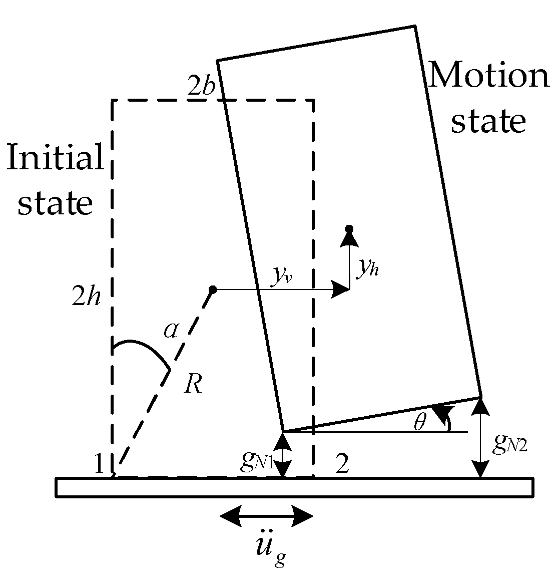
is potentially induced by vehicle braking, speed variations, and train marshalling. This excitation may cause the package to rock or slide on the base. Additionally, impacts between the bottom of the package and the vehicle during rocking can lead to the package jumping. The motion states and parameter definitions of a freestanding package under horizontal acceleration are illustrated in
Figure 1. Here, 2
h and 2
b represent the height and width of the package, respectively,
m denotes the package mass, and
α is the slenderness angle of the package, where tan
α =
b/
h. The state of the package is described by the vector
q = [
yh,
yv,
θ]
T, where
yh and
yv are the horizontal and vertical displacements of the package, and
θ is its rotation angle. The corresponding normal displacements of points 1 and 2 are denoted by
gN1 and
gN2. The interaction between the package and the vehicle can be modeled as a multibody motion problem with unilateral contact. The motion equations of rocking package can be derived using the Newton–Euler equations:
Here,
represents the vehicle acceleration, while
M,
C, and
K denote the mass, damping, and stiffness matrices of the package–vehicle impact system, respectively. The vector
f includes external forces, damping forces, and elastic forces.
WN and
WT are direction matrices of contact force and constraint in the normal and tangential directions, respectively.
λN and
λT represent the normal and tangential contact force vectors of the impact system. For the package–vehicle impact system illustrated in
Figure 1, the matrices and vectors in Equation (1) are defined as follows:
where
IG is moment of inertia of the package about the center of gravity,
IG = (1/3)
mR2, and
R2 =
h2 +
b2.
Denoting the time instants immediately before and after the impact as
t− and
t+, respectively, Equation (1) is integrated over the time interval [
t−,
t+]. During the integration of Equation (1) over the infinitesimal time interval [
t−,
t⁺], we consider only the impulsive forces as contributing to the impact dynamics, in accordance with standard impact theory. Vector
f only contains the non-impulsive forces; then, the impulses are simply the time integrals of contact forces
λN and
λT. Therefore, we obtain
From the integration of Equation (1), we obtain:
Multiplying Equation (4) by the matrices
WNT and
WTT, where the superscript T denotes the matrix transpose, letting
and
represent the normal and tangential velocities of the package relative to the vehicle base after the impact, respectively, we obtain:
where
In package transportation, ensuring transport safety requires measures to prevent cargo sliding in vehicles. Common measures include applying high-friction materials between packages and vehicle surfaces and installing anti-sliding barriers or blocks to restrict displacement. Therefore, assuming the friction coefficient between the package and the vehicle is sufficiently large to prevent sliding motion, we have
. From Equation (3), we can derive Equation (7):
Here, the Newton contact law is employed to characterize the velocity variation of package impact point:
, where
and
represent the normal velocities of the package impact point after and before the impact, respectively, and
εN is the restitution coefficient, ranging from 0 (fully plastic impact) to 1 (fully elastic impact). Defining the velocity jump at the package impact point, we obtain:
Combining Equations (6)–(8), we obtain:
E is the identity matrix.
When package sliding is considered, additional potential motion states emerge during transportation. In Equation (5), , and thus, Equation (7) no longer holds. To fully characterize the system dynamics, the relationship between tangential and normal motion must be derived. This analysis will enable the determination of possible complex motion states, presenting an interesting direction for future research.
As illustrated in
Figure 1, the package and vehicle collide at either point 1 or point 2. At the rotating pivot point of the package, because the package maintains contact with the vehicle, therefore, the velocity jump at the pivot point
vNi = 0, the normal impulse force at this point
ΛNi > 0, and the following condition holds:
On the other hand, if the package and vehicle collide at either point 1 or point 2, because the package loses contact from the vehicle at this point, therefore, the velocity jump at this point
vNi > 0, the normal impulse force at this point
ΛNi = 0, and the following condition is satisfied:
Equations (10) and (11) can be concluded as:
where
vN = [
vN1,
vN2] and
ΛN = [
ΛN1,
ΛN2]
T.
The freestanding package is placed on a moving vehicle and subjected to horizontal acceleration
, and the package begins to rotate around pivot point 1, assuming that the friction at point 1 is sufficient to prevent sliding motion. At the time instant
t−, the package collides with the vehicle at point 2, leading to the following condition:
Here,
represents the angular velocity of package about point 1 at time instant
t−. After the collision, the possible package motion states are shown in
Figure 2.
2.1. Point 1 Remains in Contact with Vehicle
After the package collides with the vehicle at point 2, if point 1 maintains contact with the vehicle, two potential cases arise:
Case 1: , if εN2 = 0; then, , and the package keeps still after collision;
Case 2: , if εN2 > 0; then, , and the package bounces and rocks around pivot point 1.
These two cases are shown in
Figure 2. Using Equations (8) and (9), we define velocity jump at points 1 and 2 in the vertical direction:
From Equation (14), vector
vN = [
vN1,
vN2]
T =
0, and by substituting vector
vN into Equation (9), we obtain:
By substituting Equation (15) into Equation (7), the tangential force induced by collision at point 1 can be obtained:
Therefore, if point 1 maintains contact with the vehicle after the collision, the friction force generated by the material between the package and the vehicle must exceed the tangential force
ΛT1 to prevent the package from sliding on the vehicle, which could compromise transportation safety. Based on Equations (12) and (15), we can conclude that if
then the package either remains stationary or rebounds around point 1 after colliding with the vehicle at point 2.
2.2. Package Rocks Around Point 2 or Detaches from Point 2
After the package collides with the vehicle at point 2, if point 1 detaches from the vehicle, there are two potential cases:
Case 1: , if εN2 = 0; then, , and the package rocks around point 2 after collision.
Case 2: , if εN2 > 0; then, , and the package detaches from the vehicle at point 1 and point 2.
These two cases are shown in
Figure 2, and the velocity jumps in the vertical direction at points 1 and 2 are:
In these two cases, since
ΛN1 = 0, by substituting Equation (18) into Equation (9) and considering Equation (12), we obtain:
By substituting Equation (19) into Equation (7), the tangential force at point 2,
ΛN2, can be determined when the package rocks around point 2:
Therefore, to prevent the package from sliding, the friction force generated by the material between the rocking package and the vehicle must exceed ΛT2.
After the package collides with the vehicle, if the package rocks around point 2 or detaches from the vehicle,
. From this, we can derive the necessary condition for the occurrence of these two scenarios:
3. Determining Collision Time Instants in Package Rocking Process
If a freestanding package rocks under the excitation of vehicle acceleration, overturning occurs when the rocking angle exceeds slenderness angle
α. This can lead to catastrophic accidents, making the analysis of rocking response and overturning risks essential. The freestanding package may rock around pivot point 1 or 2, and the governing equation of its rocking motion is:
If the package rocks around point 2, sgn(⋅) = 1; if it rocks around point 1, sgn(⋅) = −1. The frequency of the package’s rocking motion is denoted by
p, where
. Here,
IO represents the moment of inertia about point 1 or 2, given by
IO = (4/3)
mR2. During the rocking process, a collision between the package and the vehicle occurs when
θ(
t) = 0. In this case, the Newtonian contact law is applied to characterize the velocity jump of the package:
Here,
tf denotes the collision time instant, where the superscripts + and − represent the states immediately after and before the collision, respectively. The restitution coefficient can be determined based on the conservation of angular momentum:
The rocking response of the package can be determined by analyzing Equations (22) and (23). Since the rocking motion of the package is piecewise smooth and involves impacts, obtaining a closed-form solution to Equation (22) is challenging. For slender rocking blocks (where α < 15°), the governing equation of the rocking motion can be linearized, allowing the rocking response to be approximated analytically. This approach is applicable in scenarios involving slender rocking blocks, such as bridge piers or slender statues.
For non-slender blocks, Prieto et al. [
18] proposed a Dirac-delta force model to simplify the analysis of the governing differential equation. In [
19], the rocking response of the block was analyzed using an equivalent single-degree-of-freedom oscillator model. Additionally, in [
20,
21], the authors introduced an approximate method for solving nonlinear rocking motion. However, the formulation of the approximate solution is complex, making its application to the analysis of package rocking and overturning impractical.
The efficiency of analyzing the rocking motion of non-slender packages largely depends on the accurate determination of collision time instants tf. Once tf is identified, the rocking motion between collision instants becomes smooth and can be efficiently analyzed using numerical methods. In this study, we employ a time transformation method combined with the Runge–Kutta method to propose a novel approach for determining the collision time instants tf. This significantly improves the efficiency of analyzing the rocking response of the package.
As illustrated in
Figure 1, the package may rock around either point 1 or point 2. Based on Equations (22) and (23), the rocking motion of the package can be modeled as a discontinuous system with state jumps. By defining the rocking state vector
and the function
f, the system dynamics can be described as follows:
The governing equation of the package rocking motion can be rewritten as:
In Equation (26), if sgn(
θ(
t)) = −1,
f =
fα, and if sgn(
θ(
t)) = 1,
f =
fβ. From the definition of function
f in Equation (25),
fα and
fβ are smooth functions. The initial state of
x is
x(0) =
x0. From Equation (26), it can be observed that the rocking package constitutes a piecewise-smooth dynamical system [
22]. For the package rocking problem,
ψ(
x) can be written as:
where the dot · indicates the vector product. Assuming the function of initial state
ψ(
x(0)) = −
H < 0, we reduce Equation (26):
Beyond the package rocking problem, determining boundary time instants
tf that satisfy the condition
ψ(
x(
tf)) = 0 is crucial in many engineering applications. Del Buono et al. [
23] proposed a numerical procedure based on the Adams–Bashforth method, which determines
tf unidirectionally in finite steps for Equation (28). In [
24], potential conditions of midpoint distribution were considered, and a subdiagonal explicit Runge–Kutta method was employed to determine
tf unidirectionally.
In this study, we adopt the time transformation method combined with the Runge–Kutta method to propose a numerical approach for determining the time instants tf at which the rocking package collides with the vehicle. Once tf is determined, the rocking response of the package can be efficiently simulated, as the motion within each time interval defined by tf is smooth.
From Equation (27), function
ψ can be considered as a hyperplane in
x space:
where
d = [1,0,0] and
e = [0,0,0]. Since the package rocks smoothly between impact time instants
tfi, therefore, function
ψ defined in Equation (29) is monotonic and differentiable when
t ∈ [
tfi,
tfi+1],
tfi is the
ith impact time instant,
i = 0, 1, 2, …, and
t0 = 0. The following time transformation is formulated
Here, we analyze the time instants
tf at which the function
fα reaches the boundary defined by
ψ(
x) = 0. Instead of using the variable
t, we introduce the variable
s. For
t ∈ [0,
tf],
s ∈ [−
H, 0]. Based on the transformation in Equation (30), Equation (28) can be rewritten as:
Here,
ψx(
x) = ∂
ψ(
x)/∂
x. In this study, based on the time transformation in Equation (30), we utilize Equation (31) to analyze
tf instead of Equation (28). Equivalently, the trajectory
x(
s,
x0) in the
s-domain, where
s ∈ [−
H, 0], is used to simulate the package rocking motion, replacing the trajectory
x(
t,
x0) in the time domain, where
t ∈ [0,
tf]. By employing this time transformation,
tf can be determined efficiently. Let
s(−
H) =
s0 and
xgen = [
x s]
T; Equation (31) can be rewritten as:
The solution to Equation (31) can be obtained numerically using the Runge–Kutta method:
where
σ is the step size, and Σ
bi = 1, 0 ≤ ∑
ai,j ≤ 1. Similarly, the solution to Equation (32) can be obtained numerically by:
Here,
yi is defined by Equation (33). Assuming
xk+1 lies on the boundary of the function
fα, i.e.,
ψ(
xk+1) = 0, substituting
xk+1 into Equation (29) yields:
From Equation (29),
ψx(
x) =
d,
d·
g(
x) =
ψx(
x)
g(
x) = 1; therefore, Equation (35) can be rewritten as:
Based on Equation (34), if
xk+1 locates on the boundary of function
fα, we obtain:
From Equation (34) to (37), we can conclude that the boundary time instants tf of the piecewise-smooth function (26) can be determined through the time transformation (30). If a time instant tf satisfies the condition s(tf) = 0, then the corresponding response state x(tf) reaches the boundary of the function f, i.e., ψ(x(tf)) = 0.
4. Rocking Response Analysis of Freestanding Package
4.1. Numerical Analysis Algorithm for the Rocking Response
Based on the analysis in
Section 3, the collision time instant
tf of the rocking package can be determined using the time transformation method. The collision time instant satisfies the condition
s(
tf) = 0, where
s =
ψ(
x(
t)). Utilizing this principle, the numerical analysis algorithm for the rocking response of a freestanding package can be formulated as follows.
Step 1. Formulate differential equation:
The function f is defined by Equation (25), and x(0) represents the initial state of the freestanding package. The Runge–Kutta method is employed to analyze the rocking response. The time instant tk before the package collision is determined by the condition ψ(x(tk))ψ(x(tk+1)) < 0, where ψ is given by Equation (29).
Step 2. Perform time transformation t = α(s) on the time interval [tk, tf]: map interval [s0, 0] to [tk, tf], i.e., tk = α(s0) and tf = α(0). Let y(s) = x(α(s)); then y(s0) = x(tf).
If ψ(x(tk)) < 0, set s = ψ(x); the initial state is determined by s0 = ψ(x(tk)), and the function Ψ is formulated as Ψ(y(s)) = ψx(y(s))f(y(s)).
If ψ(x(tk))>0, set s = −ψ(x); the initial state is determined by s0 = −ψ(x(tk)), and the function Ψ is formulated as Ψ(y(s)) = −ψx(y(s))f(y(s)).
Formulate differential equation:
Step 3. Apply the single-step Runge–Kutta method to Equation (39); the collision time instant tf is obtained as tf = α(0). The motion state of the rocking package before the collision is given by x−(tf) = y(0). Within the time interval [0, tf], the smooth rocking response of the freestanding package can be determined using the Runge–Kutta method.
Step 4. Update the rocking motion equation: replace the rocking motion equation fα with fβ, or replace fβ with fα; reset the time instant tf to 0, and update the initial state of the rocking package as x0 = Γx−(tf).
Step 5. Iterate Steps 1 to 4 until the rocking package overturns or the response decays to a stationary state.
The flowchart of the algorithm is shown in
Figure 3.
4.2. Error of the Algorithm
Based on the formulated algorithm, the determination of the package collision time instant tf can be divided into two steps:
Step 1. Analyze the rocking response in the time interval [0, tk]:
In the time interval [0, tk], a p-order Runge–Kutta method is employed to analyze the rocking response of the freestanding package, with a time step size of σ1.
Step 2. Perform time transformation and analyze the rocking response in the time interval [tk, tf]:
In the time interval [tk, tf], the time transformation t = α(s) is applied. Within the s-interval [s0, 0], a single-step q-order Runge–Kutta method is used to analyze the package rocking response and determine the collision time instant tf. The step size for the variable s is σ2.
In Step 1, we assume the time instant before the package collision is
, and the corresponding rocking state of the package is
. Based on the error analysis of the Runge–Kutta method, the error in Step 1 can be expressed as:
In Step 2, we assume
x* is the solution of differential equation
Assuming
tf* is boundary of Equation (41) and considering the condition
ψ(
x*(
tf*)) = 0, based on Equation (39), the error in Step 2 can be expressed as:
By considering Equations (40)–(42), the analysis errors of the collision time instant and the collision condition, resulting from the algorithm proposed in this study, can be expressed as:
From Equation (43), the analysis errors of the algorithm proposed in this study are primarily influenced by the time step σ1. Reducing σ1 not only decreases the analysis error in Step 1 but also reduces |s0|, thereby minimizing the analysis error in Step 2. Additionally, the orders p and q of the Runge–Kutta method also significantly affect the overall analysis error of the proposed algorithm.
In this paper, standard fourth-order Runge–Kutta method is adopted, i.e., p = q = 4; the second- and third-order methods are also adopted for comparison.
5. Example
To validate the rocking analysis method proposed in this study, we conducted an experiment on a rocking package excited by sinusoidal base acceleration. Additionally, numerical analysis of the package rocking response under random load excitation was performed. The experimental and numerical results were then compared with the response predicted by the algorithm proposed in this paper.
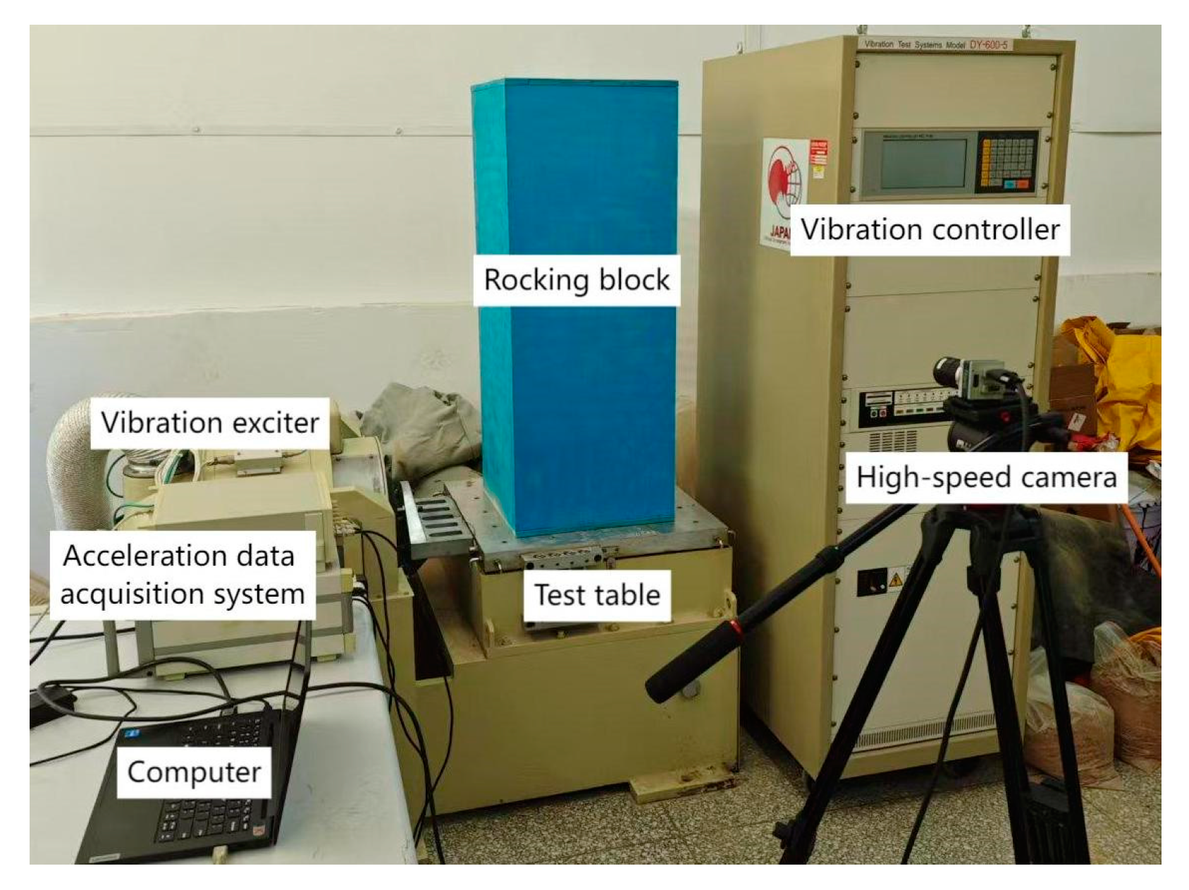
An experimental system was designed to record the response of the rocking package, as illustrated in
Figure 4. The system consists of a vibration exciter, a test table, a vibration controller, a rocking block, an acceleration data acquisition system, a high-speed camera, and other components. The vibration exciter is rotated and connected to the test table, while control parameters are set on the vibration controller to ensure that the block on the table is subjected to horizontal vibration with the desired characteristics. The block simulates the freestanding package, and the excitation acceleration on the test table is measured with an accelerometer and recorded by a computer through the acceleration data acquisition system. The high-speed camera is adjusted so that the axis of the camera lens is perpendicular to the plane of the block and passes through its centroid. The rocking motion of the package is recorded with the camera, and the rocking angle at each time instant is determined. The vibration controller is configured to apply sinusoidal excitation to the test table. Considering the transition of the excitation from the initial state to the sinusoidal state, the acceleration of the test table is expressed as:
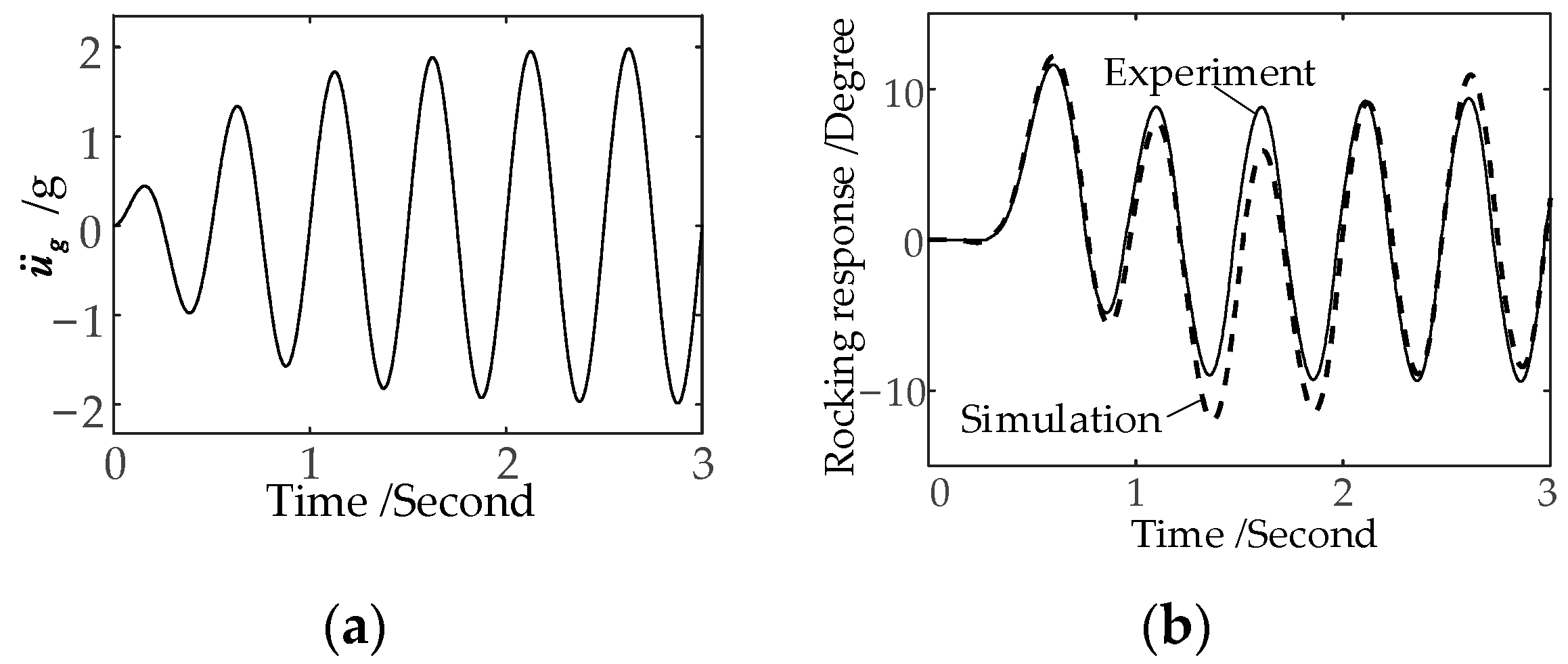
The parameters of the excitation acceleration and the block are provided in
Table 1. The acceleration of the test table is shown in
Figure 5a. The algorithm proposed in this study, based on time transformation, is applied to analyze the rocking response of the block. The rocking response predicted by the algorithm is shown in
Figure 5b, alongside the recorded rocking response obtained from the high-speed camera. From the results, it can be concluded that the proposed algorithm accurately analyzes the rocking response of the freestanding package.
In addition to sinusoidal excitation, random vibration is applied to the rocking block to further validate the proposed algorithm. The recorded random acceleration of the vehicle during transportation is shown in
Figure 6a. The algorithm proposed in this study is employed to predict the rocking response, with the time step
σ1 set to 0.01 s. The resulting rocking response of the block is presented in
Figure 6b. From the response, it is observed that the block begins to rock at
t = 5.023 s. After 15 impacts between the rocking block and the vehicle, the rocking response becomes negligible. For comparison, the second-, third-, and fourth-order Runge–Kutta methods (with a time step
σ = 0.001 s) are also used to analyze the rocking response under random vibration. The rocking response simulated by the Runge–Kutta method is convergent, the simulation error is
O(
σp+1), and
p is the order of the Runge–Kutta method. The response obtained from the Runge–Kutta method is included in
Figure 6b. The results demonstrate that the algorithm proposed in this study provides accurate predictions of the rocking response excited by random vibration.
To evaluate the accuracy and computational efficiency of the proposed method, we conducted 1000 numerical simulations of package rocking dynamics under random loading, using a time step of
σ1 = 0.01 s. For comparison, the second-, third-, and fourth-order Runge–Kutta methods were also employed, using the time step
σ = 0.001 s.
Table 2 summarizes the computational runtimes and the mean squared errors (MSEs) relative to the benchmark results obtained via the fourth-order Runge–Kutta method with a refined time step (
σ = 0.0001 s). As evidenced in
Figure 6b and
Table 2, the prediction error of the rocking response decreases with increasing order of the Runge–Kutta method, while the computational runtime exhibits a corresponding increase. Notably, the proposed algorithm achieves comparable accuracy in predicting package rocking responses while significantly reducing the computational time compared to higher-order Runge–Kutta methods.
Compared with the Runge–Kutta method and the equivalent model method, the freestanding package rocking response analysis method proposed in this study offers several advantages. It enables the determination of the exact time instant at which the package impacts the vehicle and identifies the smooth rocking response intervals. As a result, the analysis efficiency is significantly improved while maintaining good accuracy.


