
Computational Investigation of Aerodynamic Behaviour in Rubber O-Ring: Effects of Flow Velocity and Surface Topology


Abstract
1. Introduction
2. Methodology
2.1. Pre-Processing
2.1.1. Detailed Conditions and Cloning
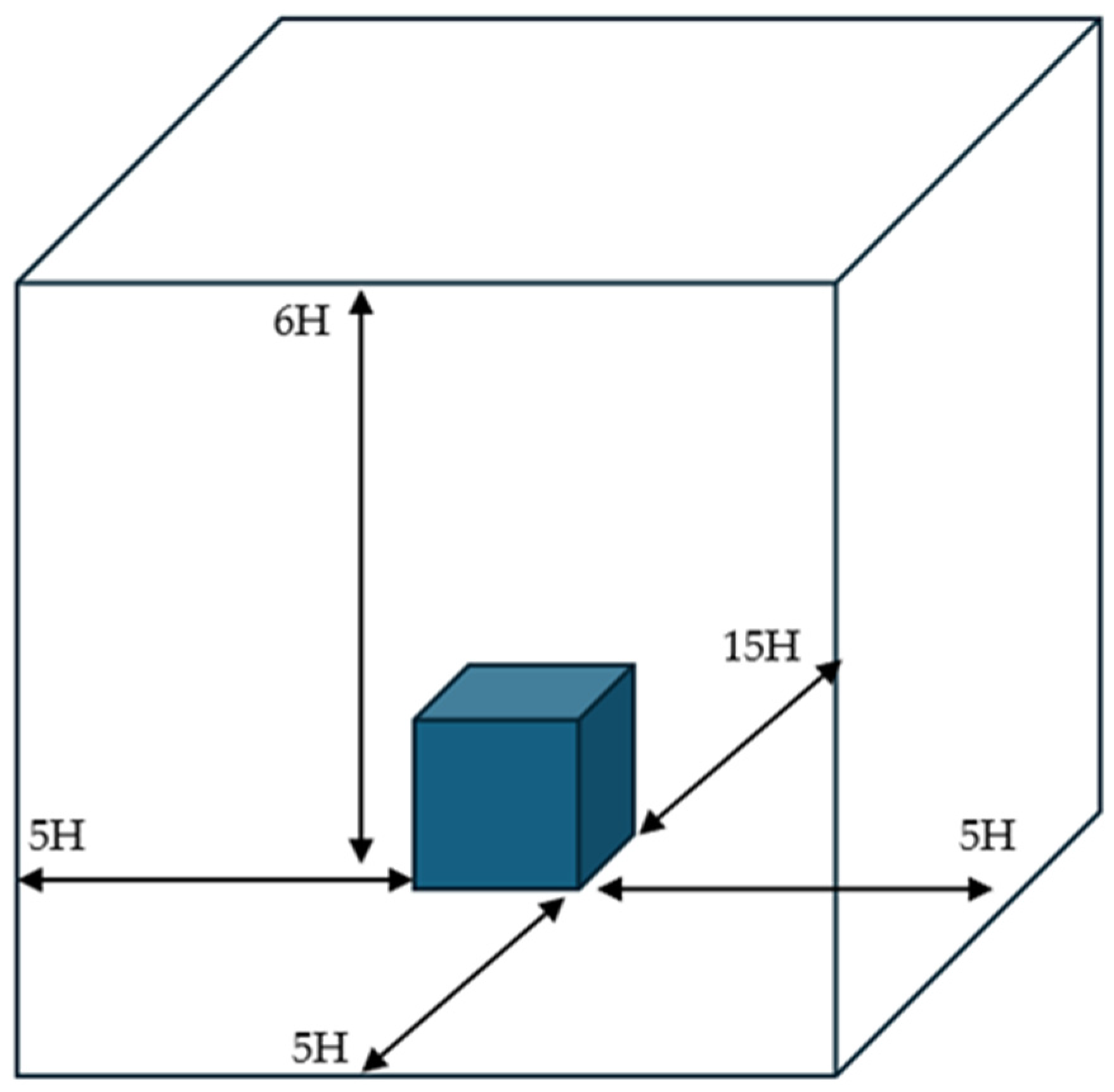
2.1.2. Computational Domain
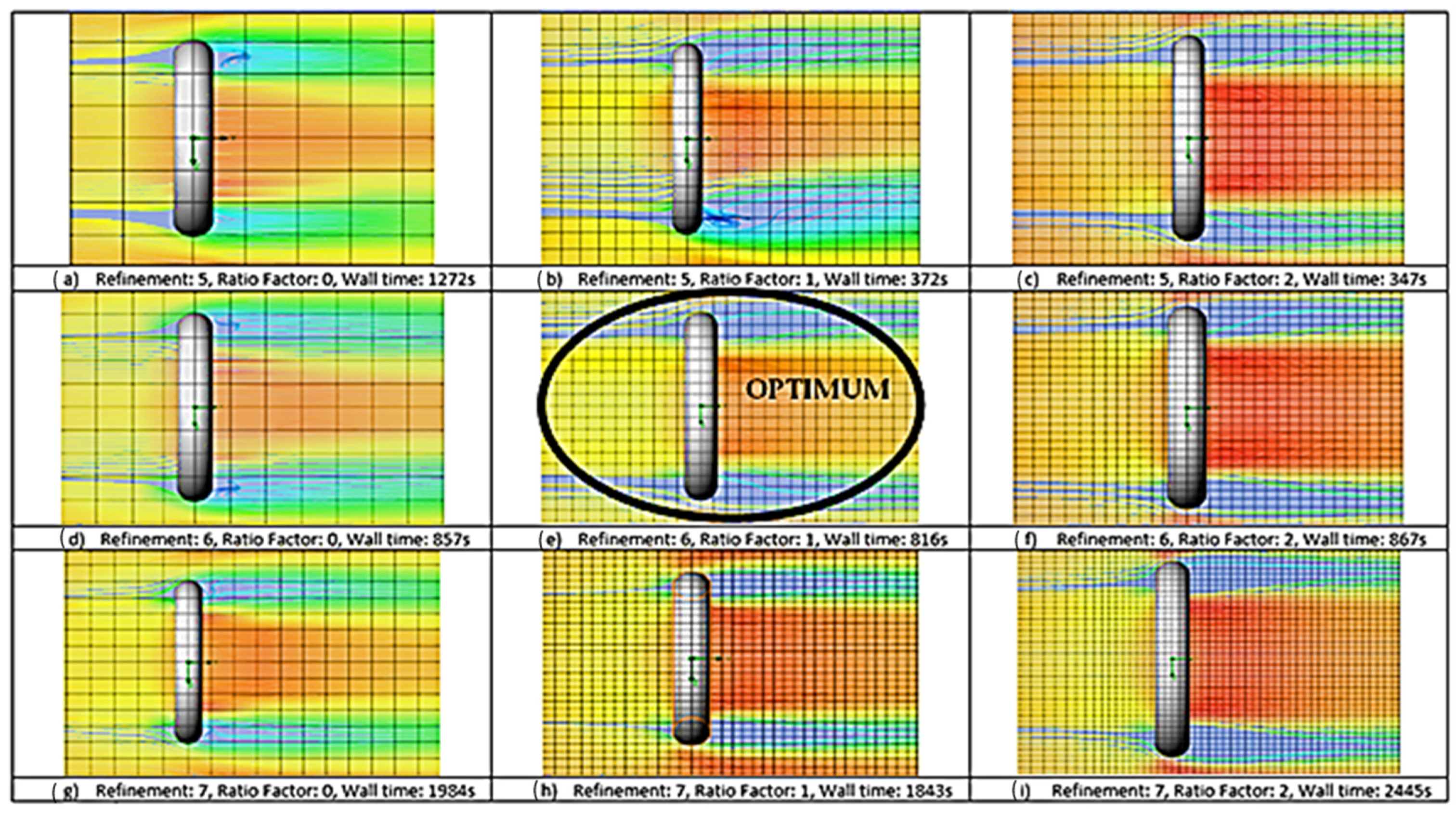
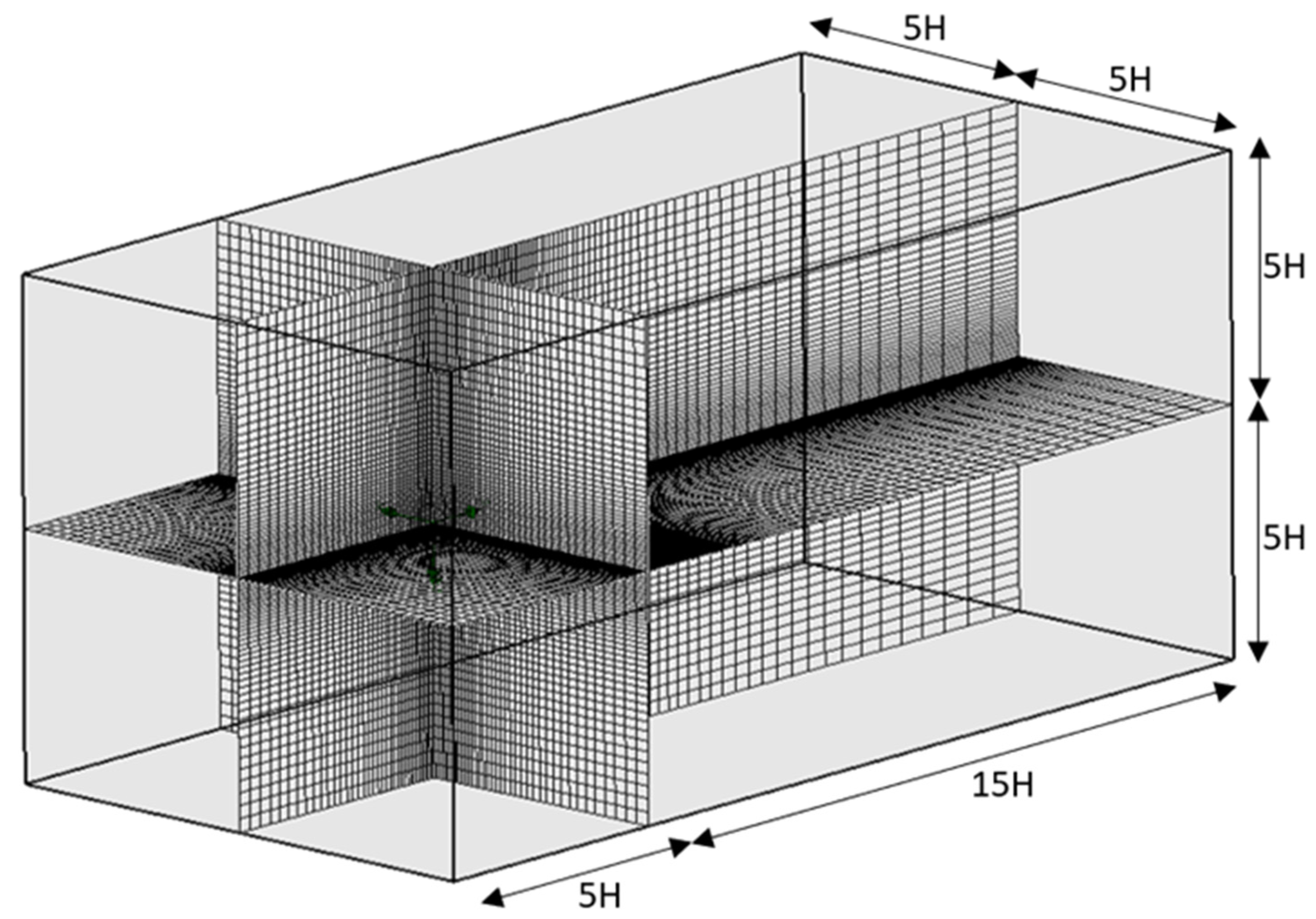
2.1.3. Mesh Generation
2.1.4. Objectives
2.2. Post-Processing
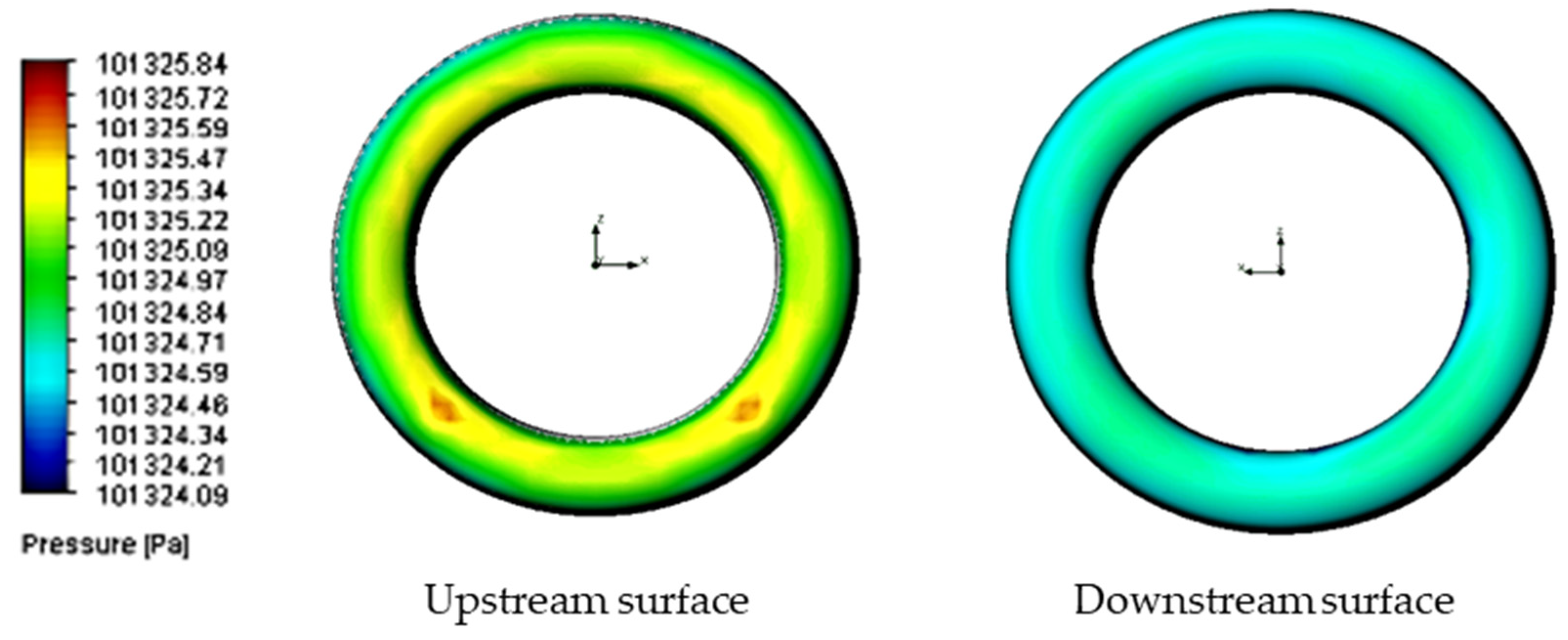
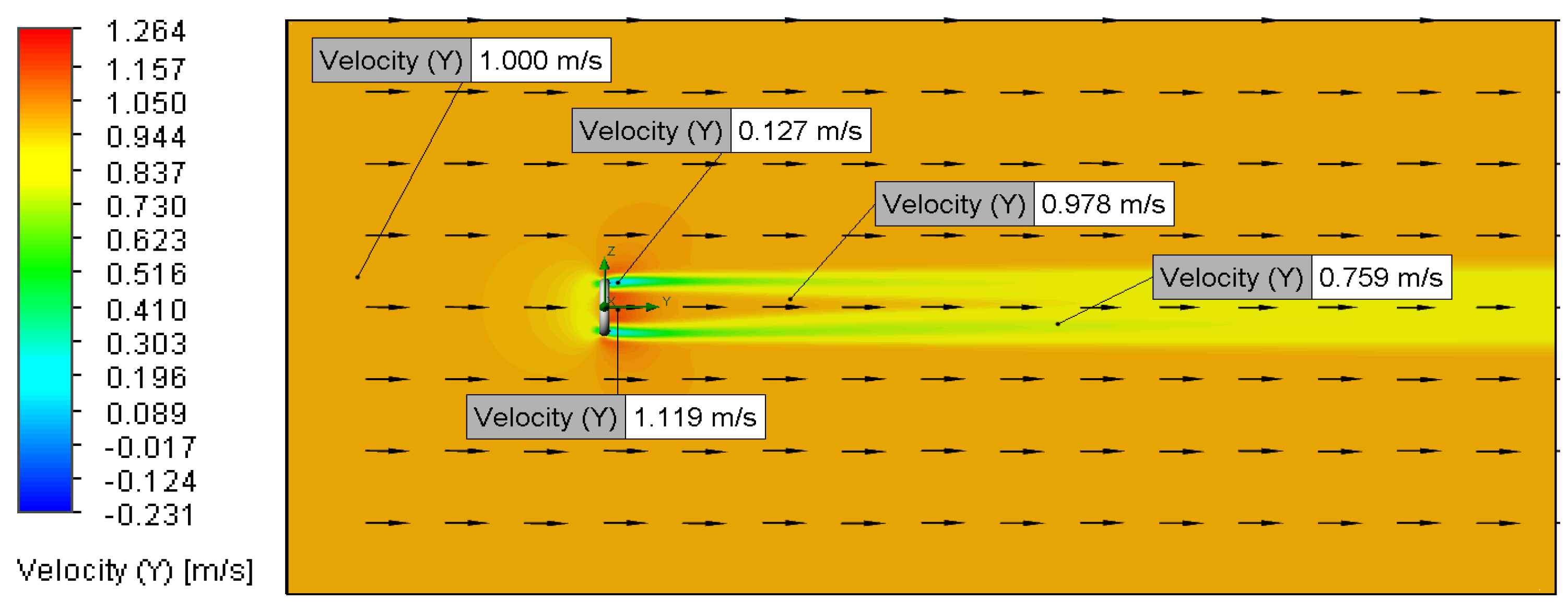
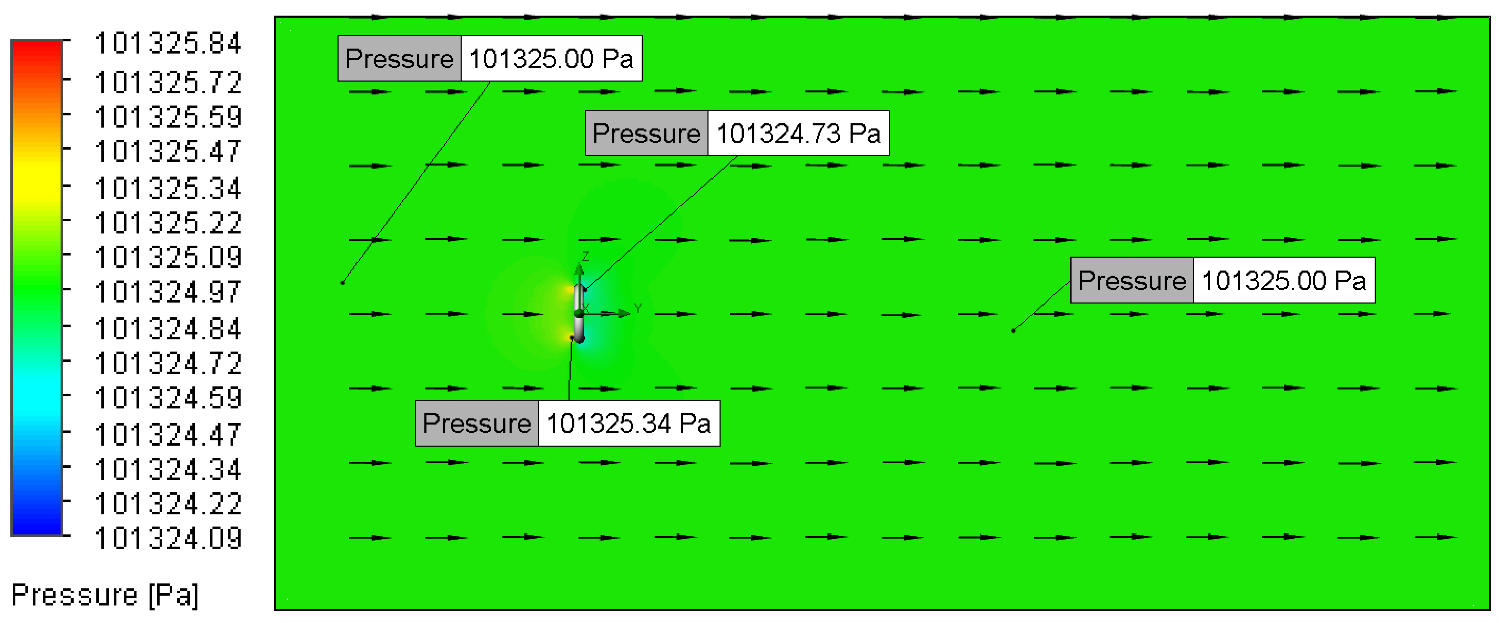
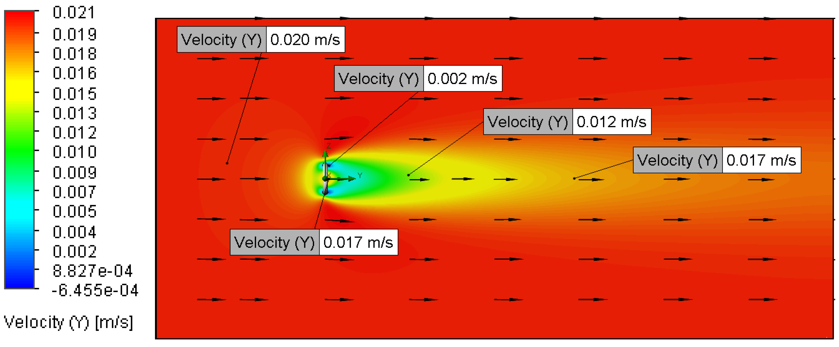
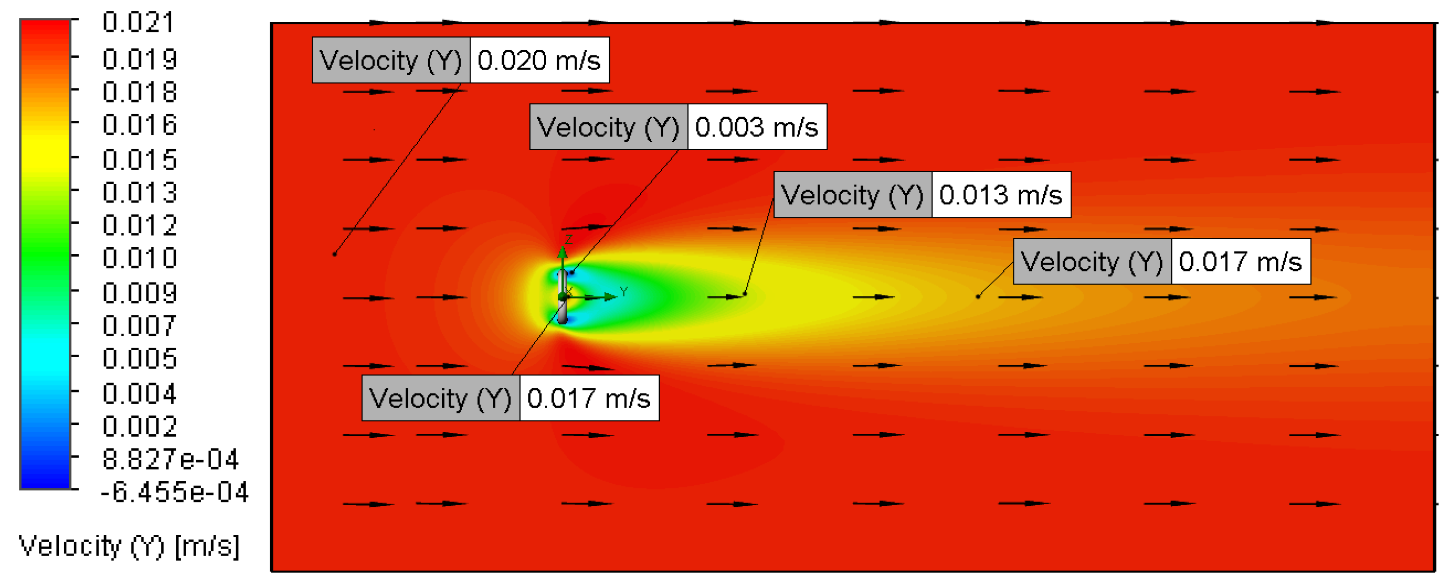
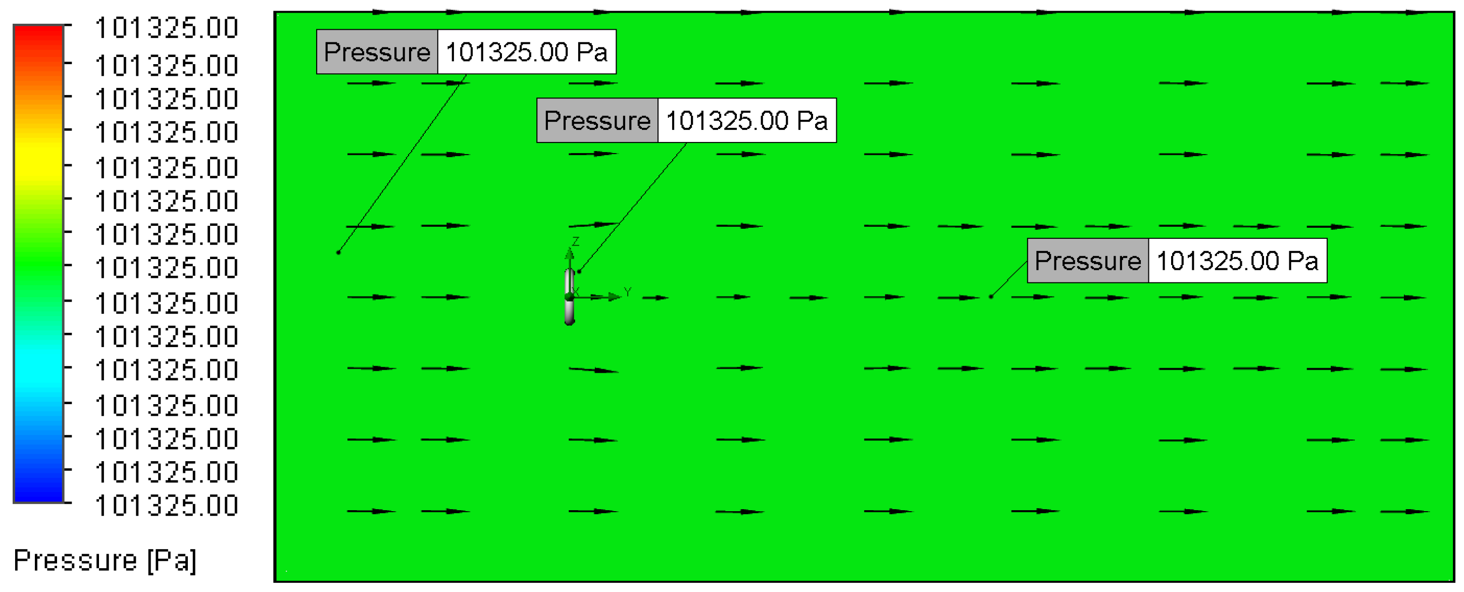
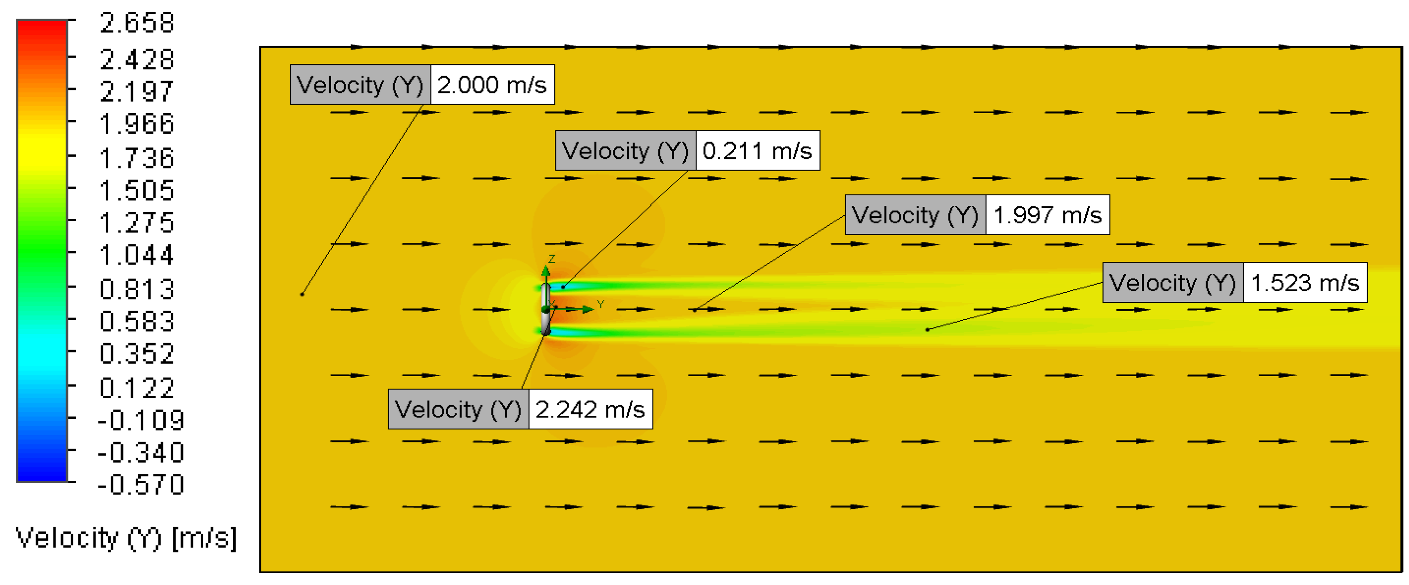
- Contour Plot: uses a colour gradient to show changes in pressure and velocity distributions, up and downstream of the O-ring.
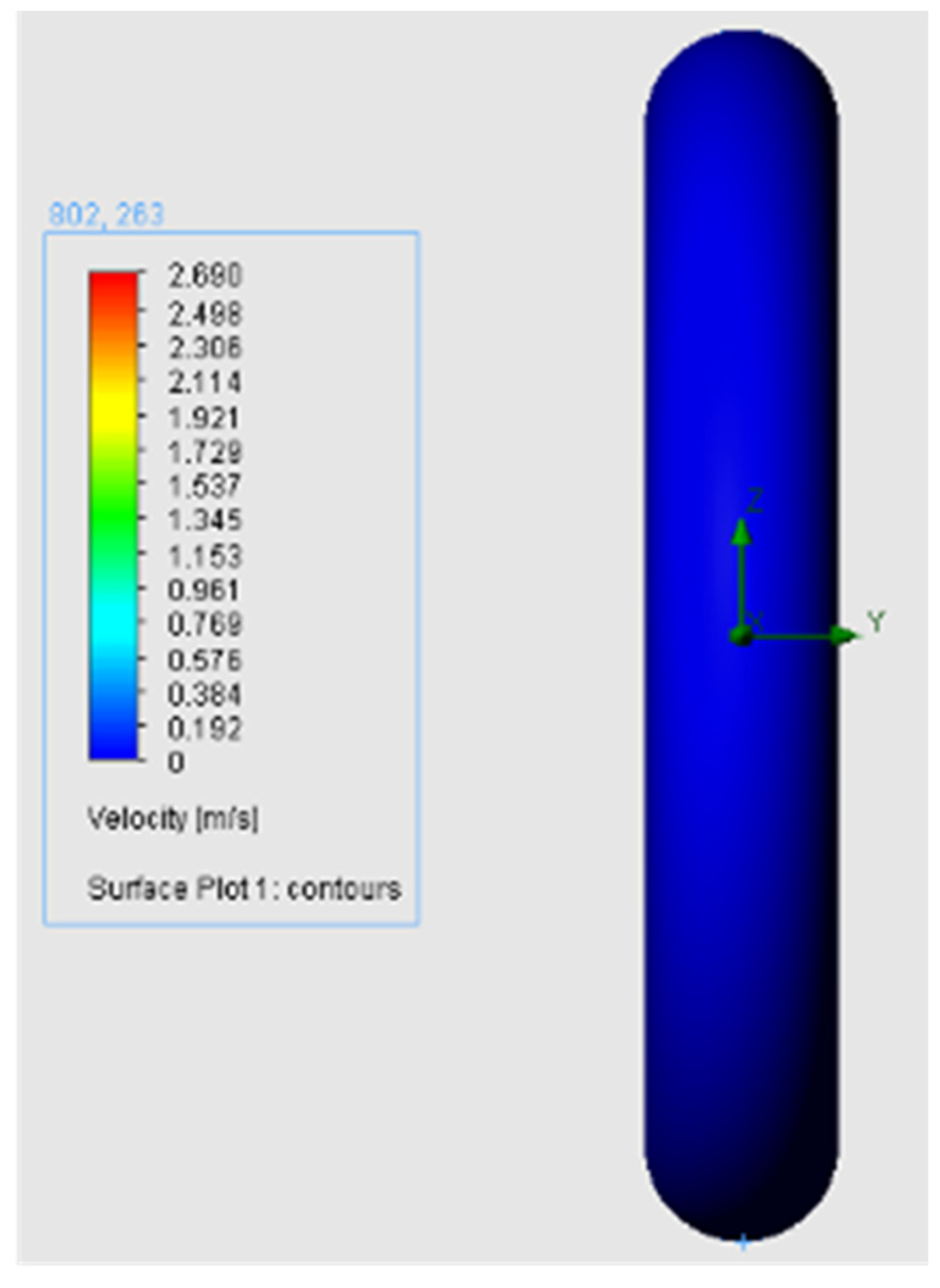
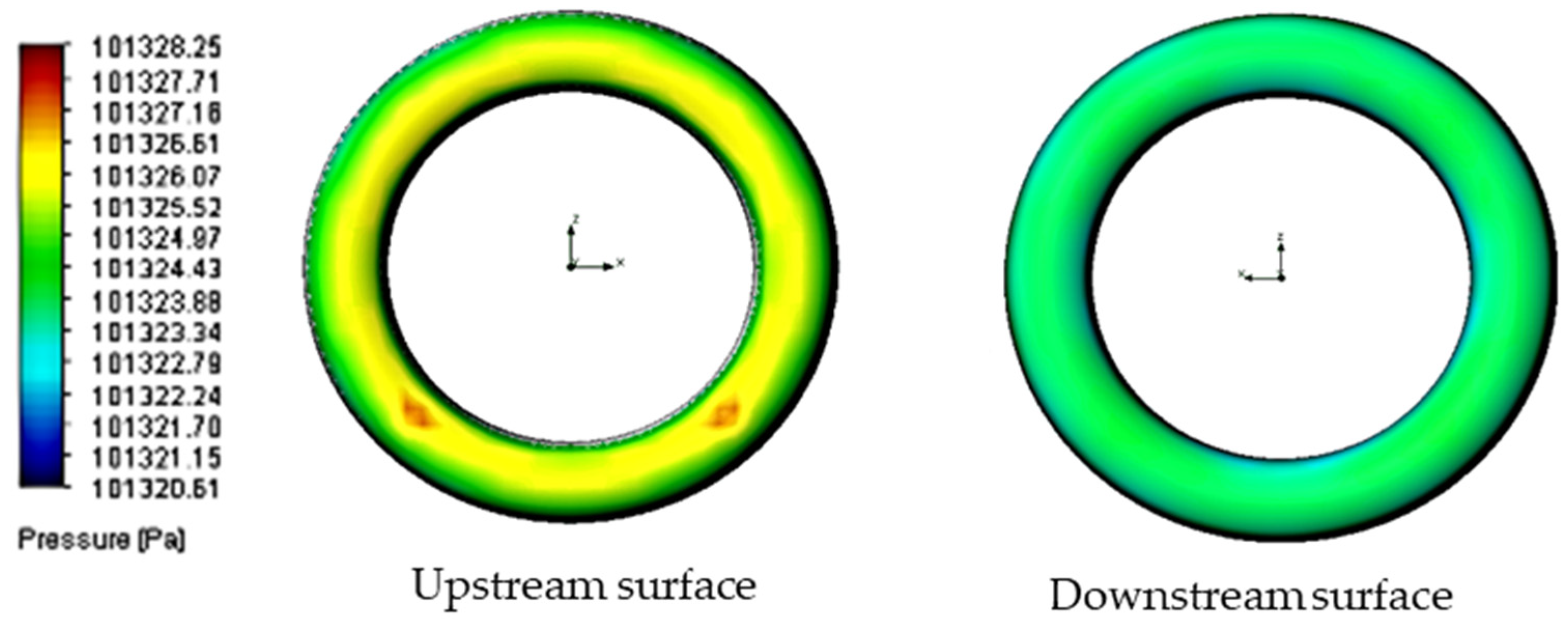
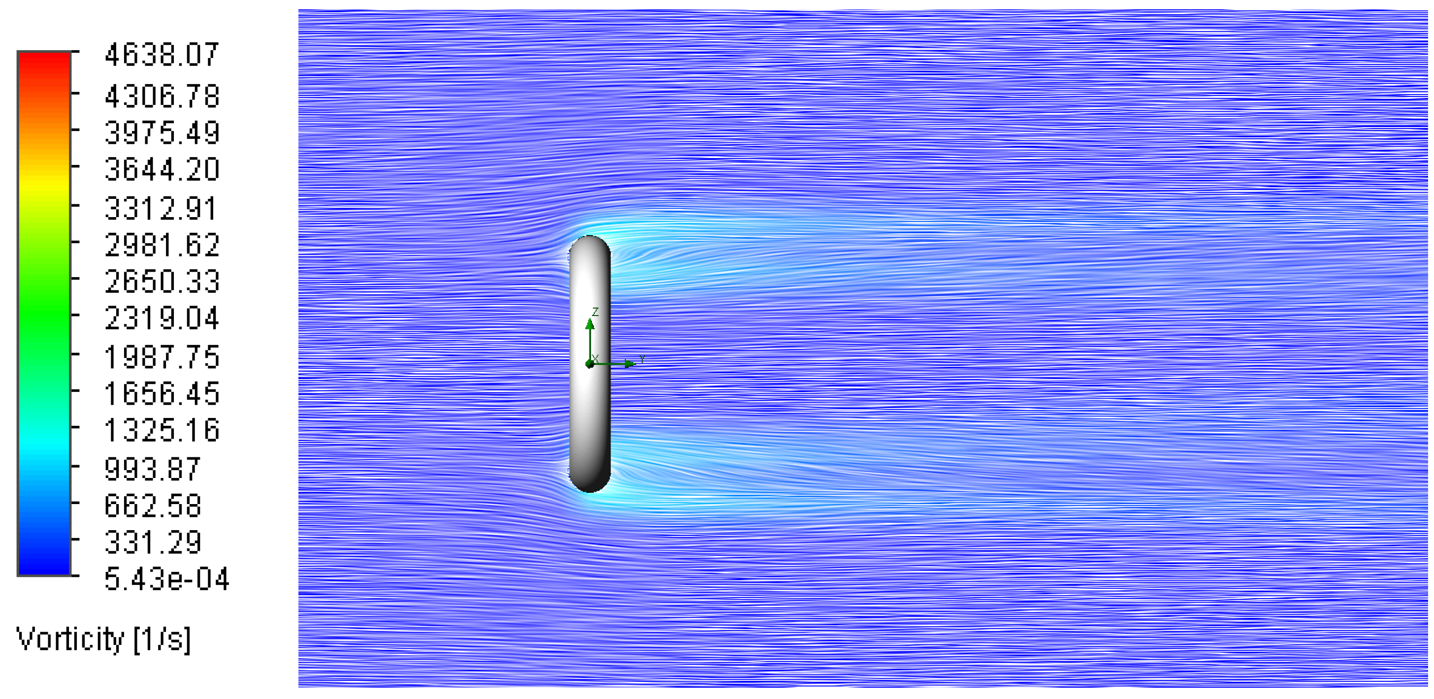
- Surface Plot: used to study the interface between the O-ring body and fluid boundary (Figure 6)
3. Results
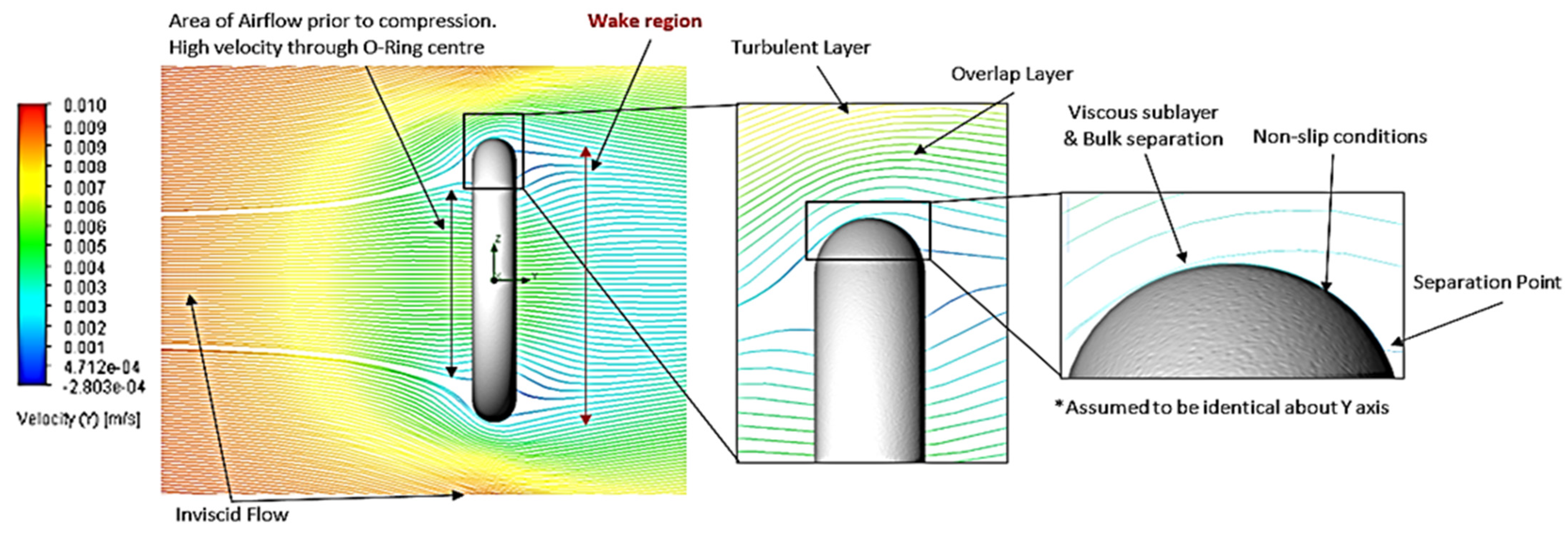
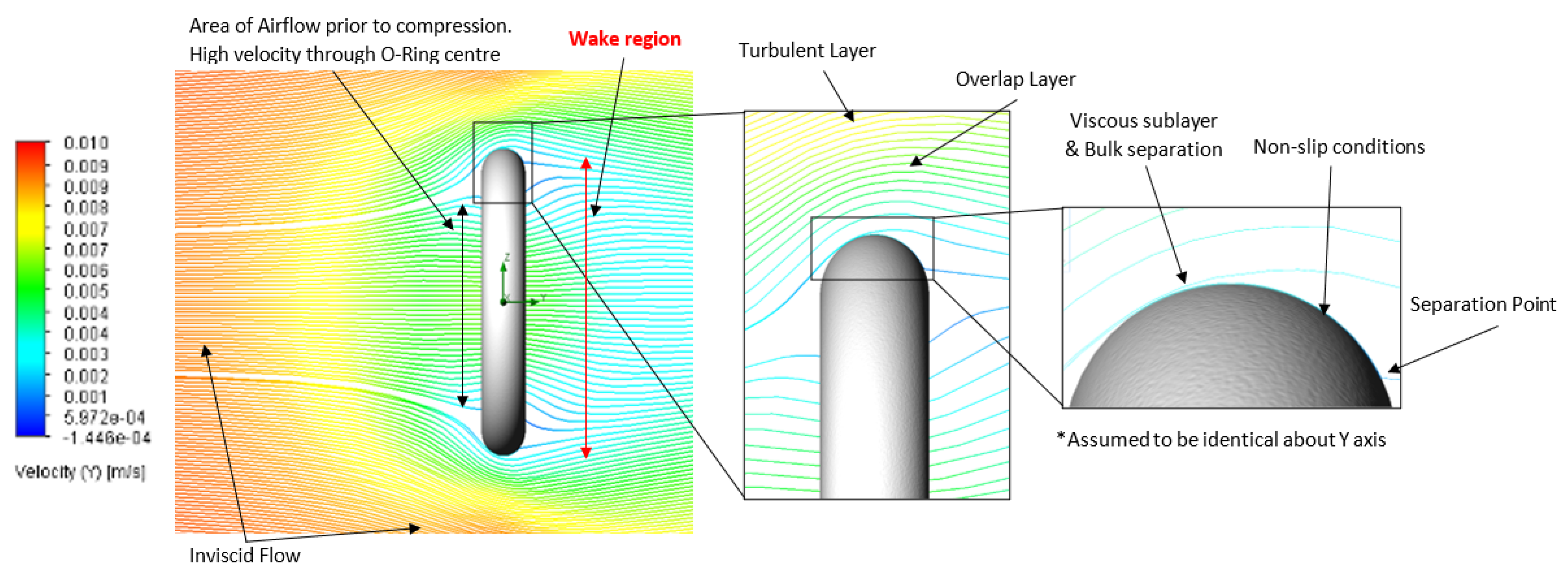
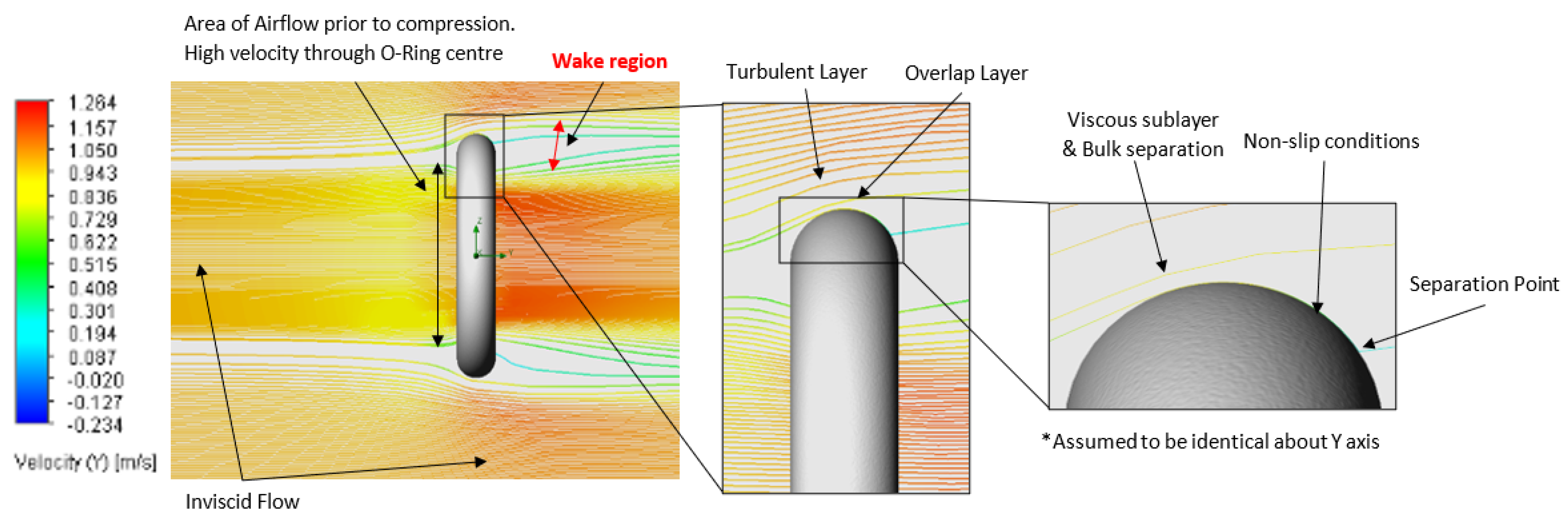
3.1. Boundary Layer
3.1.1. Relationship Between Flow Velocity and Boundary Layer
3.1.2. Relationship Between Surface Roughness and Boundary Layer
3.2. Velocity and Pressure Distribution
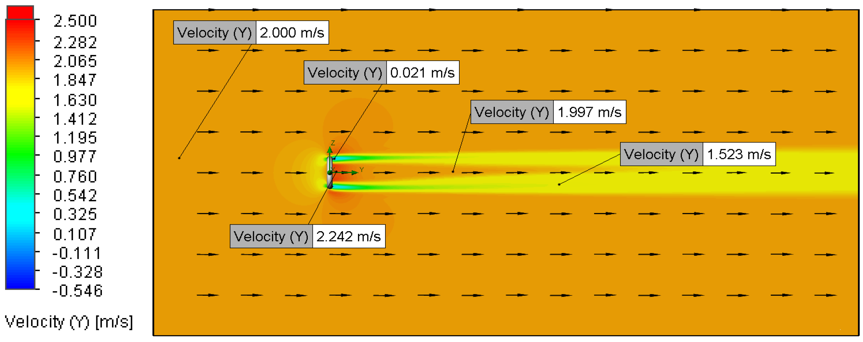
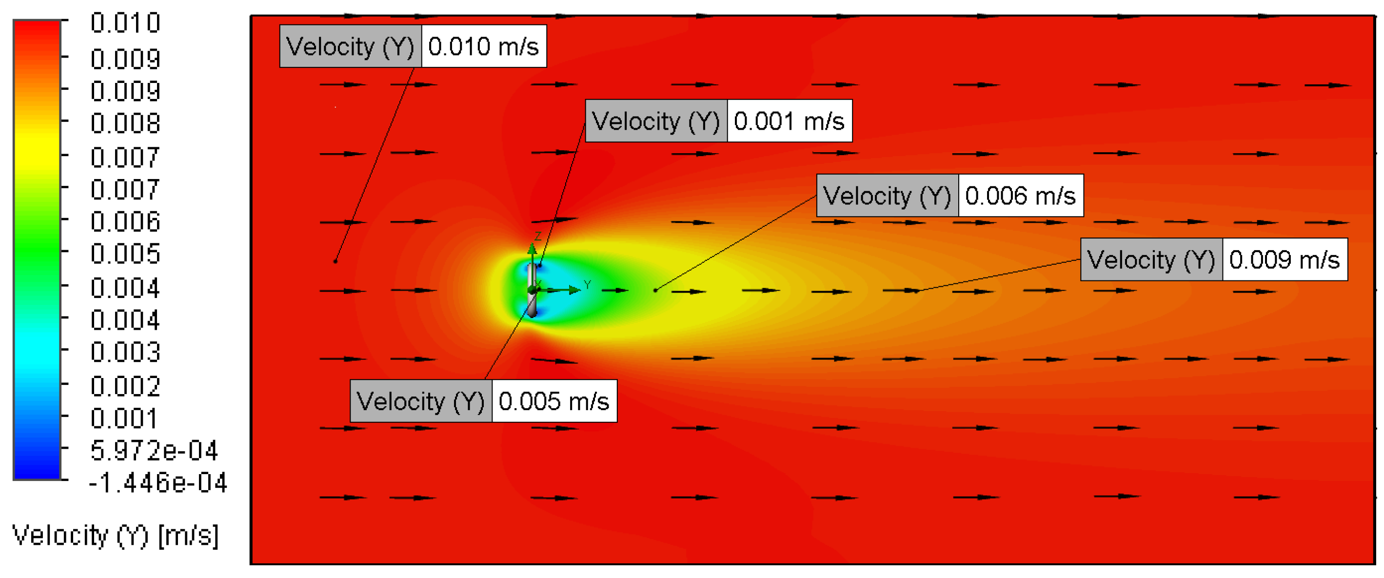
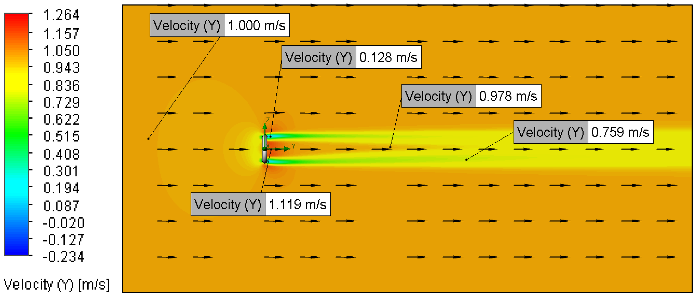
3.2.1. Relationship Between Flow Velocity and Velocity Distribution
3.2.2. Relationship Between Surface Roughness and Velocity Distribution
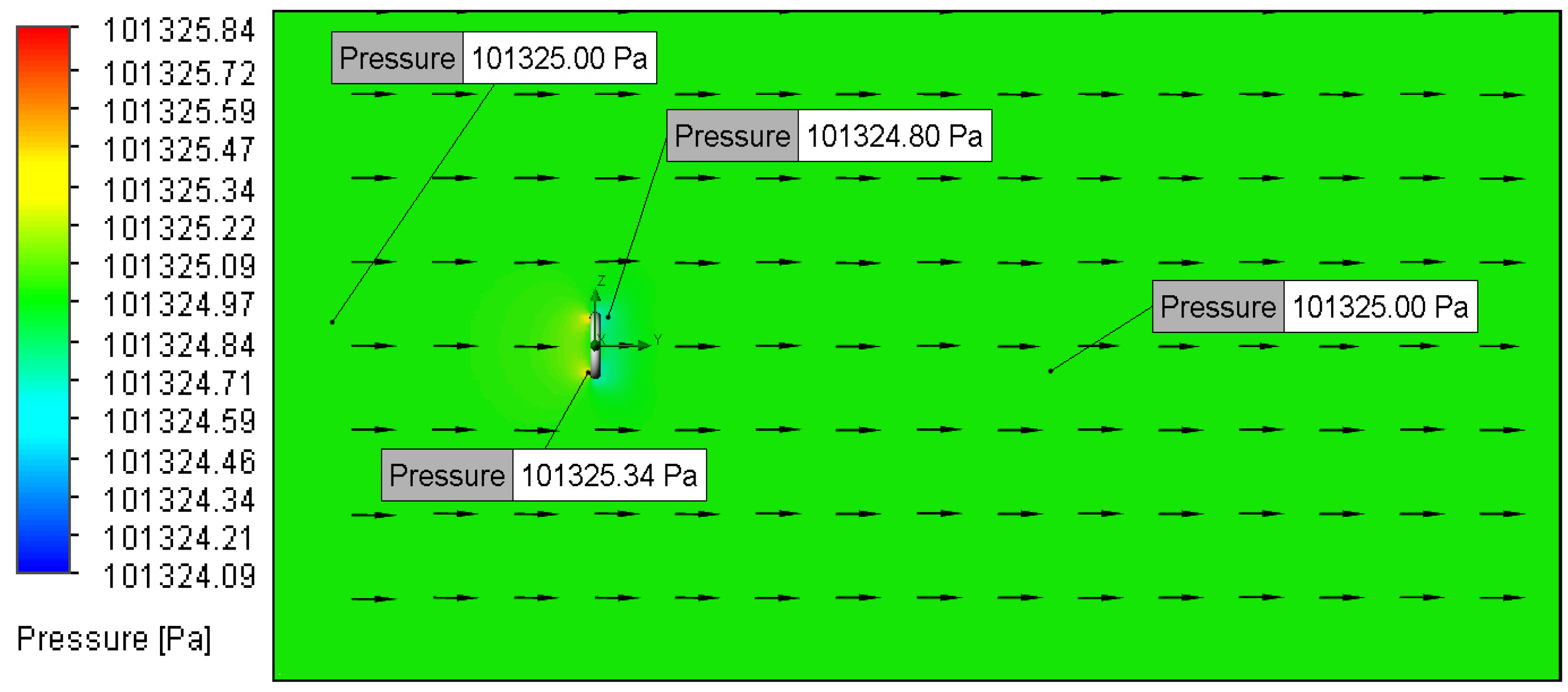
3.2.3. Relationship Between Flow Velocity and Pressure Distribution
3.2.4. Relationship Between Surface Roughness and Pressure Distribution
3.3. Vortex Shedding
Relationship Between Flow Velocity/Surface Roughness and Vorticity Concentration
3.4. Drag Coefficients
3.4.1. Relationship Between Flow Velocity and Drag Coefficients
3.4.2. Impact of Surface Roughness on Drag
4. Conclusions
Author Contributions
Funding
Institutional Review Board Statement
Informed Consent Statement
Data Availability Statement
Conflicts of Interest
References
- Anderson, J.D. Computational Fluid Dynamics. The Basics with Applications; Corrigan, J., Castellano, E., Eds.; McGraw-Hill, Inc.: Singapore, 1995; p. 547. [Google Scholar]
- Sagat, C.; Mane, P.; Gawali, B. Experimental and CFD analysis of airfoil at low Reynolds number. Int. J. Mech. Eng. Robot. Res. 2012, 1, 277–283. [Google Scholar]
- Ismail, N.; Sharudin, H.; Talib, R.; Hassan, A.; Yusoff, H. The Influence of Hoop Diameter on Aerodynamic Performance of O-Ring Paper Plane. In Proceedings of the International Conference on Aerospace and Mechanical Engineering (AeroMech17), Penang, Malaysia, 21–22 November 2017; p. 012034. [Google Scholar]
- Ladeinde, F.; Nearon, M.D. CFD applications in the HVAC&R industry. ASHRAE J. 1997, 39, 44–48. [Google Scholar]
- Xia, B.; Sun, D.-W. Applications of computational fluid dynamics (CFD) in the food industry: A review. Comput. Electron. Agric. 2002, 34, 5–24. [Google Scholar] [CrossRef]
- Matsson, J.E. An Introduction to SOLIDWORKS Flow Simulation 2021; SDC Publications: Kansas, KS, USA, 2021; p. 350. [Google Scholar]
- Revuz, J.; Hargreaves, D.; Owen, J. On the domain size for the steady-state CFD modelling of a tall building. Wind Struct. 2012, 15, 313. [Google Scholar] [CrossRef]
- Galindo, J.; Hoyas, S.; Fajardo, P.; Navarro, R. Set-up analysis and optimization of CFD simulations for radial turbines. Eng. Appl. Comput. Fluid Mech. 2013, 7, 441–460. [Google Scholar] [CrossRef]
- Bixler, B.; Pease, D.; Fairhurst, F. The accuracy of computational fluid dynamics analysis of the passive drag of a male swimmer. Sports Biomech. 2007, 6, 81–98. [Google Scholar] [CrossRef] [PubMed]
- Liu, Y.; Glass, G. Effects of Mesh Density on Finite Element Analysis; SAE Technical Paper; SAE: Warrendale, PA, USA, 2013; ISSN 0148-7191. [Google Scholar]
- Alam, F.; Steiner, T.; Chowdhury, H.; Moria, H.; Khan, I.; Aldawi, F.; Subic, A. A study of golf ball aerodynamic drag. Procedia Eng. 2011, 13, 226–231. [Google Scholar] [CrossRef]
- Mallick, M.; Kumar, A.; Tamboli, N.; Kulkarni, A.; Sati, P.; Devi, V.; Chandar, S. Study on drag coefficient for the flow past a cylinder. Int. J. Civ. Eng. Res. 2014, 5, 301–306. [Google Scholar]
- Dugdale, R.H. Fluid Mechanics, 3rd ed.; George Godwin LTD.: London, UK, 1981; p. 218. [Google Scholar]
- Richardson, S. On the no-slip boundary condition. J. Fluid Mech. 1973, 59, 707–719. [Google Scholar] [CrossRef]
- Southard, J. Structure of Turbulant Boundary Layers. Available online: https://geo.libretexts.org/Bookshelves/Sedimentology/Book%3A_Introduction_to_Fluid_Motions_and_Sediment_Transport_(Southard)/04%3A_Flow_in_Channels/4.05%3A_Structure_of_Turbulent_Boundary_Layers (accessed on 23 March 2023).
- Power, N. Boundary Layer Thickness. Available online: https://www.nuclear-power.com/nuclear-engineering/fluid-dynamics/boundary-layer/boundary-layer-thickness/ (accessed on 23 March 2023).
- Mott, R.L. Applied Fluid Mechanics, 4th ed.; Helba, S., Ed.; Prentice-Hall Inc.: Hoboken, NJ, USA, 1994; p. 581. [Google Scholar]
- Airshaper. What Is a Boundary Layer-Laminar and Turbulant Boundary Layers Explained. YouTube. 2022. Available online: https://www.youtube.com/watch?v=TwOxa9rAOfE (accessed on 7 April 2025).
- Khairani, C.; Marpaung, T. Computational analysis of fluid behaviour around airfoil with Navier-Stokes equation. In Proceedings of the 2018 International Conference on Engineering, Technologies, and Applied Sciences, Bandar Lampung, Indonesia, 18–20 October 2018; p. 012003. [Google Scholar]
- Spálenský, V.; Rozehnal, D. CFD simulation of dimpled sphere and its wind tunnel verification. MATEC Web Conf. 2017, 107, 00077. [Google Scholar] [CrossRef]
- Wu, W.; Piomelli, U. Effects of surface roughness on a separating turbulent boundary layer. J. Fluid Mech. 2018, 841, 552–580. [Google Scholar] [CrossRef]


| Setup | Analysis Type | Fluid Composition | O-Ring Material | O-Ring Topography (μm) | Fluid Velocity (m/s) |
|---|---|---|---|---|---|
| 1 | External | Air | Natural Rubber | 5 | 0.01 |
| 2 | 5 | 1.00 | |||
| 3 | 5 | 0.02 | |||
| 4 | 5 | 2.00 | |||
| 5 | 100 | 0.01 | |||
| 6 | 100 | 1.00 | |||
| 7 | 100 | 0.02 | |||
| 8 | 100 | 2.00 |
| Settings | Setup 1 | Setup 2 | Setup 3 | Setup 4 | Setup 5 | Setup 6 | Setup 7 | Setup 8 |
|---|---|---|---|---|---|---|---|---|
| Analysis Type | ||||||||
| Analysis Type | External | External | External | External | External | External | External | External |
| Physical Feature | Fluid Flow | Fluid Flow | Fluid Flow | Fluid Flow | Fluid Flow | Fluid Flow | Fluid Flow | Fluid Flow |
| Fluids | ||||||||
| Fluids | Air | Air | Air | Air | Air | Air | Air | Air |
| Flow Type | Laminar and Turbulent | Laminar and Turbulent | Laminar and Turbulent | Laminar and Turbulent | Laminar and Turbulent | Laminar and Turbulent | Laminar and Turbulent | Laminar and Turbulent |
| Wall Condition | ||||||||
| Wall Conditions | Adiabatic Wall | Adiabatic Wall | Adiabatic Wall | Adiabatic Wall | Adiabatic Wall | Adiabatic Wall | Adiabatic Wall | Adiabatic Wall |
| Roughness | 5 μm | 5 μm | 5 μm | 5 μm | 100 μm | 100 μm | 100 μm | 100 μm |
| Initial and Ambient Conditions | ||||||||
| Thermodynamic Parameters: | ||||||||
| Pressure | 101,325 Pa | 101,325 Pa | 101,325 Pa | 101,325 Pa | 101,325 Pa | 101,325 Pa | 101,325 Pa | 101,325 Pa |
| Temperature | 293.2 K | 293.2 K | 293.2 K | 293.2 K | 293.2 K | 293.2 K | 293.2 K | 293.2 K |
| Velocity Parameters: | ||||||||
| Definition | 3D Vector | 3D Vector | 3D Vector | 3D Vector | 3D Vector | 3D Vector | 3D Vector | 3D Vector |
| Velocity X | 0 | 0 | 0 | 0 | 0 | 0 | 0 | 0 |
| Velocity Y | 0.01 m/s | 1.00 m/s | 0.02 m/s | 2.00 m/s | 0.01 m/s | 1.00 m/s | 0.02 m/s | 2.00 m/s |
| Velocity Z | 0 | 0 | 0 | 0 | 0 | 0 | 0 | 0 |
| Turbulence Parameters | N/A | N/A | N/A | N/A | N/A | N/A | N/A | N/A |
| Symbol | Name | Value | Units |
|---|---|---|---|
| Density | 1.204 | kg/m3 | |
| μ | Dynamic Viscosity | 1.825 × 10⁻⁵ | Kg/ms |
| L | Characteristic Linear Dimension | 0.01492 | m |
| A | Area | 9.376 × 10⁻⁵ | m2 |
| V | Velocity | Dependant on trial | m/s |
| FN | Normal Force | Dependant on trial | N |
| FFR | Frictional Force | Dependant on trial | N |
| Symbol | Name | Value | Units |
|---|---|---|---|
| ρ | Density | 1.204 | kg/m3 |
| V1 | Initial Velocity | Dependant on trial | m/s |
| V2 | Velocity through O-Ring | Dependant on trial | m/s |
| A1 | The area before compression | Approximately: 0.00579 | m2 |
| A2 | Area through O-Ring | 0.00508 | m2 |
| Velocity (m/s) | Re | Total Fd | Frictional Fd | Total Cd | Frictional Cd | Pressure Cd |
|---|---|---|---|---|---|---|
| O-Ring Roughness 5 μm | ||||||
| 0.01 | 9.84 | 2.07 × 10⁻⁸ | 1.76 × 10⁻⁸ | 3.66 | 3.13 | 0.55 |
| 0.02 | 19.69 | 5.70 × 10⁻⁸ | 4.41 × 10⁻⁸ | 2.52 | 1.95 | 0.58 |
| 1.00 | 984.31 | 4.25 × 10⁻⁵ | 8.43 × 10⁻⁶ | 0.75 | 0.15 | 0.60 |
| 2.00 | 1968.62 | 1.59 × 10⁻⁴ | 2.39 × 10⁻⁵ | 0.71 | 0.11 | 0.60 |
| O-Ring Roughness 100 μm | ||||||
| 0.01 | 9.84 | 2.07 × 10⁻⁸ | 1.76 × 10⁻⁸ | 3.66 | 3.12 | 0.55 |
| 0.02 | 19.69 | 5.70 × 10⁻⁸ | 4.41 × 10⁻⁸ | 2.52 | 1.95 | 0.58 |
| 1.00 | 984.31 | 4.25 × 10⁻⁵ | 8.47 × 10⁻⁶ | 0.75 | 0.15 | 0.60 |
| 2.00 | 1968.62 | 1.59 × 10⁻⁴ | 2.39 × 10⁻⁵ | 0.71 | 0.11 | 0.60 |
Disclaimer/Publisher’s Note: The statements, opinions and data contained in all publications are solely those of the individual author(s) and contributor(s) and not of MDPI and/or the editor(s). MDPI and/or the editor(s) disclaim responsibility for any injury to people or property resulting from any ideas, methods, instructions or products referred to in the content. |
© 2025 by the authors. Licensee MDPI, Basel, Switzerland. This article is an open access article distributed under the terms and conditions of the Creative Commons Attribution (CC BY) license (https://creativecommons.org/licenses/by/4.0/).
Share and Cite
Singleton, T.; Saeed, A.; Khan, Z.A. Computational Investigation of Aerodynamic Behaviour in Rubber O-Ring: Effects of Flow Velocity and Surface Topology. Appl. Sci. 2025, 15, 5006. https://doi.org/10.3390/app15095006
Singleton T, Saeed A, Khan ZA. Computational Investigation of Aerodynamic Behaviour in Rubber O-Ring: Effects of Flow Velocity and Surface Topology. Applied Sciences. 2025; 15(9):5006. https://doi.org/10.3390/app15095006
Chicago/Turabian StyleSingleton, Thomas, Adil Saeed, and Zulfiqar Ahmad Khan. 2025. "Computational Investigation of Aerodynamic Behaviour in Rubber O-Ring: Effects of Flow Velocity and Surface Topology" Applied Sciences 15, no. 9: 5006. https://doi.org/10.3390/app15095006
APA StyleSingleton, T., Saeed, A., & Khan, Z. A. (2025). Computational Investigation of Aerodynamic Behaviour in Rubber O-Ring: Effects of Flow Velocity and Surface Topology. Applied Sciences, 15(9), 5006. https://doi.org/10.3390/app15095006