Design of Cislunar Navigation Constellation via Orbits with a Resonant Period

Abstract

With the increasing number of cislunar space missions, real-time and reliable navigation and communication services have become critical. It is necessary to develop the navigation constellations dedicated to cislunar space services. However, there are plenty of orbits in cislunar space providing alternative orbits, which makes constellation design a challenging task. To address this, this paper proposes a method for a cislunar navigation constellations configuration design via orbits with resonant periods. First, a periodic orbit catalog for the Earth–Moon system is constructed. Baseline orbits are selected from different orbital families, and all resonant orbits with periods proportional to the baseline orbits are compiled into a resonant orbit set. Second, a Dilution of Precision (DOP) model for navigation performance and a spatial zoning model are established. Then, resonant orbital combinations are screened based on orbital type composition, followed by resonance constellation generation according to predetermined constellation scales. All constellation configurations are categorized by orbital type to obtain a full resonant constellation set. Finally, the proposed method is applied to design optimal configurations providing navigation services for near-Earth and lunar regions. The simulation results shows that constellations combining L2 southern/northern Near-Rectilinear Halo Orbits (NRHOs) with vertical orbits at L4/L5 points deliver the optimal navigation performance in cislunar regions. The relationships between orbital radius and DOP values in target areas, as well as the DOP evolution patterns over constellation periods, are analyzed. The mean DOP values of the optimal constellation in both the near-Earth region and the lunar region increase as the spatial radius expands.

1. Introduction

The cislunar region is the space between the Earth and Moon, encompassing the area extending from Geostationary Earth Orbit (GEO, approximately 36,000 km) to lunar orbit (approximately 384,400 km). This domain holds strategic significance for deep space exploration, lunar development, and the future space economy. With the growing demand for cislunar space exploration and development, reliable real-time communication and navigation services have become essential for crewed lunar missions [1], robotic lunar surface operations, precise orbit determination [2,3], asteroid detection [4,5], and deep space exploration missions [6,7,8,9]. Current deep space exploration missions predominantly rely on the existing ground-based Deep Space Network (DSN) infrastructure, while autonomous deep space navigation systems fall far short of the required precision levels [10,11]. Moreover, surging mission demands risk overwhelming the DSN’s operational capacity. This has intensified research into developing navigation and positioning systems for deep space missions through leveraging cislunar periodic orbits or lunar orbital architectures.

Farquhar et al. [12] first proposed deploying navigation and communication satellites at Earth–Moon libration points to construct constellations. Carpenter et al. [13] analyzed the navigation and coverage capabilities of constellations near the Earth–Moon L2 point for lunar orbiters, demonstrating that four libration point satellites at L2 could achieve higher navigation accuracy than the Deep Space Network. Romagnoli and Circi [14] introduced a Lunar Global Positioning System (LGPS) and Lunar Global Communication System (LGCS), utilizing Lissajous orbits at Earth–Moon L1/L2 points. Circi [15] extended this work to Halo orbits, proposing LGPS architectures using northern/southern Halo orbit families near L1/L2. Chinese scholars have also contributed extensively to cislunar constellation research. Xu et al. [16] suggested deploying cislunar communication constellations on retrograde periodic orbits near Earth–Moon L2/L3/L4/L5 points to achieve full coverage of Earth and lunar surfaces. Meng and Chen [17] conducted a comprehensive design and analysis of libration point navigation constellations, considering orbital selection, spatial coverage, Geometric Dilution of Precision (GDOP), signal transmission, and navigation accuracy. Zhang and Xu [18] derived candidate constellations (e.g., L245 three-satellite and L1245 four-satellite configurations) that meet all the cislunar coverage requirements based on L2/L4/L5 point geometries. Peng et al. [19] proposed Earth–Moon satellite constellation designs using multi-revolution elliptic Halo orbits (ME-Halo) near L2 within an elliptic restricted three-body problem framework. Additionally, orbital resonance phenomena in near-Earth constellations have been investigated. Sampaio et al. [20] studied the resonance between satellite orbital periods and Earth’s rotation period using GPS as a case study. Lee et al. [21] optimized regional coverage constellations by analyzing revisit resonance in coverage performance under periodic requirements. Current Earth–Moon navigation constellation designs face challenges including heterogeneous orbital types, non-uniform design parameters, and excessive optimization search spaces, with existing methods being limited to localized cislunar regions rather than providing full-space coverage. This paper addresses these limitations through a period resonance-based constellation design, enabling full-cycle performance analysis and simplified system management/optimization.

This work introduces a method for generating optimal navigation resonance constellations targeting distinct cislunar regions via the construction of an operational database and DOP evaluation. Key innovations include the following: (1) a classification strategy prioritizing the baseline orbit, which is the trajectory with the minimal orbital period within the resonant constellation and intra-constellation orbital type composition in the Earth–Moon–Spacecraft three body system, enabling the systematic generation and categorization of resonant combinations into constellations; (2) the identification of optimal resonant configurations for near-Earth and lunar systems; and (3) an analysis of DOP distributions over time and the orbital radius.

The paper is structured as follows: Section 2 details the circular restricted three-body problem (CRTBP) dynamics, CRTBP-based operational orbit database generation, DOP calculation formulas, and definitions/gridding methods for critical cislunar regions. Section 3 comprehensively describes the resonance constellation design methodology using the orbit database. Section 4 applies this method to derive five superior and five inferior constellations across target regions, with case studies analyzing the relationships between orbital radius/DOP values and temporal DOP evolution in the combined region. The conclusions provide actionable recommendations for the implementation of an Earth–Moon navigation constellation.

2. Fundamental Theory

2.1. Circular Restricted Three-Body Problem

The orbital design for the constellation in this paper was established using the three-body problem, with the most typical simplified problem being the CRTBP. This problem is based on two important assumptions, as follows: (1) it is assumed that the primary bodies $P_1$ and $P_2$ have masses $M_1$ and $M_2$, respectively, and the mass of the target spacecraft $P_3$ is m, where m is much smaller than $M_1$ and $M_2$; (2) the motion of $P_1$ and $P_2$ around the system barycenter is a Keplerian circular orbit, meaning the distance between $P_1$ and $P_2$ is constant. The expressions for the CRTBP model are typically represented in a rotating coordinate system, which is defined as a dynamic system according to the motion of the two primary bodies. The origin O is located at the barycenter of the Earth–Moon system; the X-axis always points from the barycenter to $P_2$, the Z-axis points in the direction of the system’s angular momentum, perpendicular to the Earth–Moon motion plane and pointing towards the North Celestial Pole, and the Y-axis is determined using the right-hand rule.

For computational convenience, it is necessary to perform normalization of the CRTBP problem. The normalized length unit is the distance between the two primary bodies, denoted as

$$L^{*}=D_1+D_2$$

(1)

In the Earth–Moon system, the characteristic length is defined as $L^{*}=\mathrm{384,400}$ km. The normalized mass unit is set as the sum of the two primary masses (Earth and Moon), denoted as

$$m^{*}=M_1+M_2$$

(2)

The normalized time is defined as

$$t^{*}=\sqrt{{\displaystyle \frac{{L^{*}}^3}{G{m}^{*}}}}$$

(3)

The unit of $t^{*}$ is second. In cislunar dynamical modeling, the standard practice avoids the direct utilization of celestial mass parameters. Instead, gravitational parameters (GM) are adopted to eliminate uncertainties associated with the gravitational constant (G). As calibrated by the JPL DE440 ephemeris, the normalized GM values are defined as $G{M}_1=\mathrm{398,600.435}$ km³/s² for Earth and $G{M}_2=4902.8001$ km³/s² for the Moon, demonstrating enhanced precision in orbital numerical integration. In subsequent analyses, all variables and dimensionless quantities undergo normalization through division by their characteristic reference values, except when explicitly accompanied by dimensional unit annotations.

Additionally, a critical parameter in the CRTBP is the mass ratio $\mu$, defined as the ratio of the secondary body’s mass to the total system mass, expressed as

$$\mu ={\displaystyle \frac{M_2}{m^{*}}}={\displaystyle \frac{G{M}_2}{G{M}_1+G{M}_2}}$$

(4)

The dimensionless equations of motion for the CRTBP in the rotating frame are provided as follows:

$$\left\{\begin{array}{c}\ddot{x}-2\dot{y}-x=-{\displaystyle \frac{\left(1-\mu \right)\left(x+\mu \right)}{{∥{\overrightarrow{r}}_{13}∥}^3}}-{\displaystyle \frac{\mu \left(x-\left(1-\mu \right)\right)}{{∥{\overrightarrow{r}}_{23}∥}^3}}\hfill \\ \ddot{y}+2\dot{x}-y=-{\displaystyle \frac{\left(1-\mu \right)y}{{∥{\overrightarrow{r}}_{13}∥}^3}}-{\displaystyle \frac{\mu y}{{∥{\overrightarrow{r}}_{23}∥}^3}}\hfill \\ \ddot{z}=-{\displaystyle \frac{\left(1-\mu \right)z}{{∥{\overrightarrow{r}}_{13}∥}^3}}-{\displaystyle \frac{\mu z}{{∥{\overrightarrow{r}}_{23}∥}^3}}\hfill \end{array}\right.$$

(5)

where ${\overrightarrow{r}}_{13}$ denotes the normalized vector from the primary body $P_1$ to $P_3$ in the rotating frame, ${\overrightarrow{r}}_{13}=\left[\begin{array}{ccc}x+\mu & y& z\end{array}\right]$. ${\overrightarrow{r}}_{23}$ denotes the normalized vector from the primary body $P_2$ to $P_3$ in the rotating frame, ${\overrightarrow{r}}_{23}=\left[\begin{array}{ccc}x-(1-\mu )& y& z\end{array}\right]$.

2.2. Earth–Moon System’s Periodic Orbit Database Generation

Libration points in the Earth–Moon system host a variety of periodic orbits with significant application potential. DROs (Distantly Retrograde Orbits) near the Moon represent a class of periodic orbits with substantial engineering value [22]. Algorithms for constructing these orbits under the CRTBP framework follow the methods presented in Refs. [23,24,25,26,27]. Leveraging these references, this study generates multiple orbit families to build a CRTBP periodic orbit library, forming the operational database for constellation design.

North–south Halo orbit families near collinear points exhibit identical period distributions due to their XY-plane symmetry; thus, north Halos serve as baseline orbits for resonant constellation design. Similarly, L4 and L5 orbits are XZ-plane symmetric with matching periods, so L4 orbits are adopted as the baseline for periodic-resonant configurations.

Key implementation details include the following:

• DROs [22]: DROs are planar periodic orbits in the lunar vicinity, which are symmetric around the X-axis of the Earth–Moon rotating frame. These orbit families are generated through natural parameter continuation methods. They have an initial x-direction amplitude of 1000 km, which is continued along +X with step size $1\times {10}^{-4}$.
• Lyapunov and orbits: Lyapunov orbits constitute planar periodic trajectories near the collinear libration points that maintain X-axis symmetry in the Earth–Moon rotating frame. Their families are similarly constructed via natural parameter continuation. They have the same parameters as DROs but these continue along −X for L1/L3.
• Halo and Vertical orbits: Halo orbit families and vertical orbit families represent non-planar periodic solutions near collinear libration points, exhibiting symmetry about the XZ-plane. These are extended via Ref. [23]’s method, starting from z-direction amplitudes of 1000 km. The normalized continuation step size for x/z-directions at each collinear point is $1\times {10}^{-4}$.

Orbits near triangular libration points are extended using the pseudo-arclength continuation method. Planar orbits have an initial amplitude of 10,000 km, while vertical orbits start with 1000 km. Likewise, the normalized continuation step size is $1\times {10}^{-4}$.

To systematically categorize constellation types, the orbit families participating in resonant constellation generation are encoded, as shown in

Table 1. Specification and coding of orbit types in the Operational Orbit Library.

Type Num	Position	Type	Code	Minimum Period/${\mathit{t}}^{*}$	Maximum Period/${\mathit{t}}^{*}$
1	Moon	DRO	DRO	2.7261	5.9373
2	L1	Lyapunov	L1L	2.6930	7.4280
3		North Halo	L1NH	1.8037	2.7875
4		South Halo	L1SH	1.8037	2.7875
5		Vertical	L1V	2.7695	5.6891
6	L2	Lyapunov	L2L	3.3735	6.1671
7		North Halo	L2NH	1.3739	3.4155
8		South Halo	L2SH	1.3739	3.4155
9		Vertical	L2V	3.5177	5.7857
10	L3	Lyapunov	L3L	6.2184	6.2272
11		North Halo	L3NH	6.2356	6.2391
12		South Halo	L3SH	6.2356	6.2391
13		Vertical	L3V	6.2499	6.2502
14	L4	Planar	L4P	6.2832	6.2869
15		Vertical	L4V	6.5391	6.5827
16	L5	Planar	L5P	6.2832	6.2869
17		Vertical	L5V	6.5391	6.5827

, which lists the minimum and maximum orbital periods for each type.

Based on orbital period magnitudes, this study classifies orbits in resonant constellations into baseline orbits and resonant orbits. As indicated in the table, orbital types eligible as baseline orbits include DROs, all periodic orbits at L1, and Halo orbits at L2, while other types are restricted to resonant roles.

2.3. Navigation Performance Modeling

Current metrics for evaluating constellation performance include coverage, visibility, and DOP, with DOP being a critical indicator for assessing the positioning accuracy of navigation constellations. DOP reflects the error characteristics in pseudorange-based positioning solutions. Numerous studies have utilized DOP for the design and optimization of constellations; the evaluation methodologies are extensively investigated in Refs. [28,29,30]. This study accordingly analyzes the DOP performance of resonant constellations.

To ensure position resolution, constellation satellites must establish communication links with receivers to transmit pseudorange signals [31]. By definition, DOP-based solutions require the simultaneous geometric visibility of at least four satellites to the receiver. This work assumes geometric visibility (lines of sight unobstructed by large celestial bodies) as the link criterion, disregarding practical communication constraints. DOP values are computed only when a receiver achieves four-satellite visibility, with the calculation formula following standard definitions.

In the Earth–Moon rotating frame, the unit vector $\overline{\mathit{r}}$ from the user receiver to the i-th constellation satellite is expressed as

$$\overline{\mathit{r}}=\left[\begin{array}{ccc}{\displaystyle \frac{x_i-x}{R_i}}& {\displaystyle \frac{y_i-y}{R_i}}& {\displaystyle \frac{z_i-z}{R_i}}\end{array}\right]$$

(6)

where $R_i$ represents the distance between the receiver and the i-th constellation satellite.

$$R_i=\sqrt{{\left(x_i-x\right)}^2+{\left(y_i-y\right)}^2+{\left(z_i-z\right)}^2}$$

(7)

Assuming $n\left(n\ge 4\right)$ satellites in the constellation are engaged in the positioning solution at a specific epoch, the pseudorange measurement residual matrix $\mathit{H}$ is computed.

$$\mathit{H}=\left[\begin{array}{cccc}{\displaystyle \frac{x_1-x}{R_1}}& {\displaystyle \frac{y_1-y}{R_1}}& {\displaystyle \frac{z_1-z}{R_1}}& 1\\ {\displaystyle \frac{x_2-x}{R_2}}& {\displaystyle \frac{y_2-y}{R_2}}& {\displaystyle \frac{z_2-z}{R_2}}& 1\\ \dots & \dots & \dots & 1\\ {\displaystyle \frac{x_n-x}{R_n}}& {\displaystyle \frac{y_n-y}{R_n}}& {\displaystyle \frac{z_n-z}{R_n}}& 1\end{array}\right]$$

(8)

The first three columns of the matrix represent the components of the unit vector from the receiver to each constellation satellite, while the last element in each row corresponds to the partial derivative of the pseudorange with respect to the user clock bias. The covariance matrix is computed via the least squares method:

$$\mathit{Q}={\left({\mathit{H}}^T\mathit{H}\right)}^{-1}=\left[\begin{array}{cccc}{\sigma }_x^2& {\sigma }_{xy}& {\sigma }_{xz}& {\sigma }_{xt}\\ {\sigma }_{xy}& {\sigma }_y^2& {\sigma }_{yz}& {\sigma }_{yt}\\ {\sigma }_{xz}& {\sigma }_{yz}& {\sigma }_z^2& {\sigma }_{zt}\\ {\sigma }_{xt}& {\sigma }_{yt}& {\sigma }_{zt}& {\sigma }_t^2\end{array}\right]$$

(9)

In navigation constellations, the Position Dilution of Precision (PDOP) and GDOP are key metrics, denoted as $D_p$ and $D_g$ respectively. Their relationships are given by the following:

$$D_p=\sqrt{{\sigma }_x^2+{\sigma }_y^2+{\sigma }_z^2}$$

(10)

$$D_g=\sqrt{{\sigma }_x^2+{\sigma }_y^2+{\sigma }_z^2+{\sigma }_t^2}$$

(11)

This study focuses on Position PDOP, where a smaller PDOP value indicates reduced positioning errors and a superior constellation performance.

2.4. Target Area Definition and Gridding

To compute performance metrics, spatial gridding is implemented, where the performance values at the grid nodes approximate those in their vicinity. Target areas can be defined using either cuboidal spatial grids or spherical spatial grids, as follows:

• Cuboidal grids are typically applied to global spatial domains (e.g., the entire Earth–Moon system).
• Spherical grids are suited for local regions (e.g., near the Earth or the Moon).

The cuboidal spatial grid model is defined within the Earth–Moon rotating frame, with coordinate ranges along the three axes specified to delineate the spatial domain. For instance, the X-axis extends from the initial coordinate $X_0$ towards $X_f$. A schematic of the gridded cuboidal spatial domain is illustrated in Figure 1.

For such a cuboidal spatial grid, uniform discretization can be performed along each axis with specified step sizes. For example, the step size in the X-direction is denoted as $dX$. The coordinate set P of all grid points is generated as follows:

$$P=\left\{\left(x,y,z\right)\left|x=X_0+n_x·dX,y=Y_0+n_y·dY,z=Z_0+n_z·dZ\right.\right\}$$

(12)

where $n_x=0,1,\dots ,⌊{\displaystyle \frac{X_f-X_0}{dX}}⌋$, $n_y=0,1,\dots ,⌊{\displaystyle \frac{Y_f-Y_0}{dY}}⌋$, $n_z=0,1,\dots ,⌊{\displaystyle \frac{Z_f-Z_0}{dZ}}⌋$. Here, $⌊·⌋$ denotes the floor function. The cuboidal grid model enables the description of cuboidal subregions centered at any spatial point within a unified coordinate system. Let the center point coordinates be $P_0=\left(x_0,y_0,z_0\right)$; the coordinate set is then updated as follows:

$$P=\left\{\left(x,y,z\right)\left|x=X_0+n_x·dX+x_0,y=Y_0+n_y·dY+y_0,z=Z_0+n_z·dZ+z_0\right.\right\}$$

(13)

The spherical spatial grid is defined within a rotating coordinate frame using longitude, latitude, and radial distance. A schematic of the spherical gridding is shown in Figure 2.

Within this framework, longitude is defined as $\alpha \in {\left[0,360\right]}^{\circ }$ and latitude as $\delta \in {\left[-90,90\right]}^{\circ }$. To define the target spherical region, specify the spherical radius R, longitude bounds (start ${\alpha }_0$, end ${\alpha }_f$), and uniform angular step $d\alpha$. Similarly, latitude bounds (start ${\delta }_0$; end ${\delta }_f$) and step $d\delta$ must be defined. The spherical grid coordinate set P is then generated as follows:

$$P=\left\{\left(\alpha ,\delta ,R\right)\left|\alpha ={\alpha }_0+n_{\alpha }·d\alpha ,\delta ={\delta }_0+n_{\delta }·d\delta \right.\right\}$$

(14)

To facilitate computational analysis, spherical coordinates (longitude and latitude) must be converted to Cartesian coordinates. Assuming the spherical center is located at $P_0=\left(x_0,y_0,z_0\right)$, the transformation formulas are as follows:

$$P=\left\{\left(x,y,z\right)\left|x=Rcos\delta cos\alpha +x_0,y=Rcos\delta sin\alpha +y_0,z=Rsin\delta +z_0\right.\right\}$$

(15)

This study focuses on two key regions: the Earth-centered spherical region and the Moon-centered spherical region within the Earth–Moon rotating frame. The Earth’s position in this frame is defined as ${\mathit{r}}_e=\left(-\mu ,0,0\right)$, with $R_e$ denoting the radius of the Earth-centered spherical region. Similarly, the Moon’s position is ${\mathit{r}}_m=(1-\mu ,0,0)$, and $R_m$ represents the radius of the Moon-centered spherical region. These definitions enable localized navigation analyses in near-Earth and lunar proximity environments using a unified coordinate framework.

3. Design Methodology

The cislunar space offers a diverse selection of operational orbits with significant variations in orbital periods. The orbits of different periods exhibit distinct dynamic characteristics and performance advantages in specific regions. If the orbits within a constellation demonstrate resonant characteristics, the navigation and positioning performance metrics for targets will follow periodic variation patterns. This feature not only provides theoretical insights into the evolutionary mechanisms of constellation performance but also significantly streamlines the daily management, maintenance procedures, and long-term optimization strategies of the constellation system.

The cislunar resonant constellation design method proposed in this study was developed based on a lunar-periodic orbit library, comprising three main phases—orbit library preprocessing, resonance combination generation, and resonant constellation formation—as illustrated in Figure 3. During the orbit preprocessing phase, the characteristic period extraction and sorting of orbit families is implemented to isolate suitable reference orbit families for subsequent operations. The resonance combination generation phase initiates with the selected reference orbits, focusing on matching resonant orbits as core elements. Given the computational complexity caused by the large number of generated resonance combinations, a type-based merging and deduplication process is applied to orbit compositions. Finally, resonant constellations are constructed from the combinations according to predefined scale requirements, with category-based merging implemented to reduce the computational load. The optimal constellation configuration is determined through exhaustive evaluation iterations.

It is important to note that the resonant constellation design proposed in this study adheres to the following principles: (1) no more than one orbit from each orbital family is included in the constellation configuration, and (2) each orbit accommodates only one satellite.

3.1. Orbital Library Preprocessing

The first step involves preprocessing the operational orbit library. Each orbital family is sorted in ascending order of their periods, and the minimum and maximum periods for each orbital family are recorded. Assuming there are N orbital families, a characteristic period matrix $\tilde{\mathit{P}}$ of size $N\times 3$ is defined, where each row vector corresponds to the following:

$${\tilde{\mathit{p}}}_i=\left[\begin{array}{ccc}min\left({\mathit{P}}_i\right)& max\left({\mathit{P}}_i\right)& I_i\end{array}\right]$$

(16)

Here, ${\mathit{P}}_i$ denotes the period vector of the i-th orbital family, and $I_i$ represents its identifier. The matrix $\tilde{\mathit{P}}$ is then sorted by the first column (minimum periods) in ascending order. The largest element in the second column of $\tilde{\mathit{P}}$, denoted as $P_m$, indicates the maximum period across the entire orbit library. This process establishes the period ranges for all orbital families, completing the preparatory phase for the resonant constellation generation algorithm.

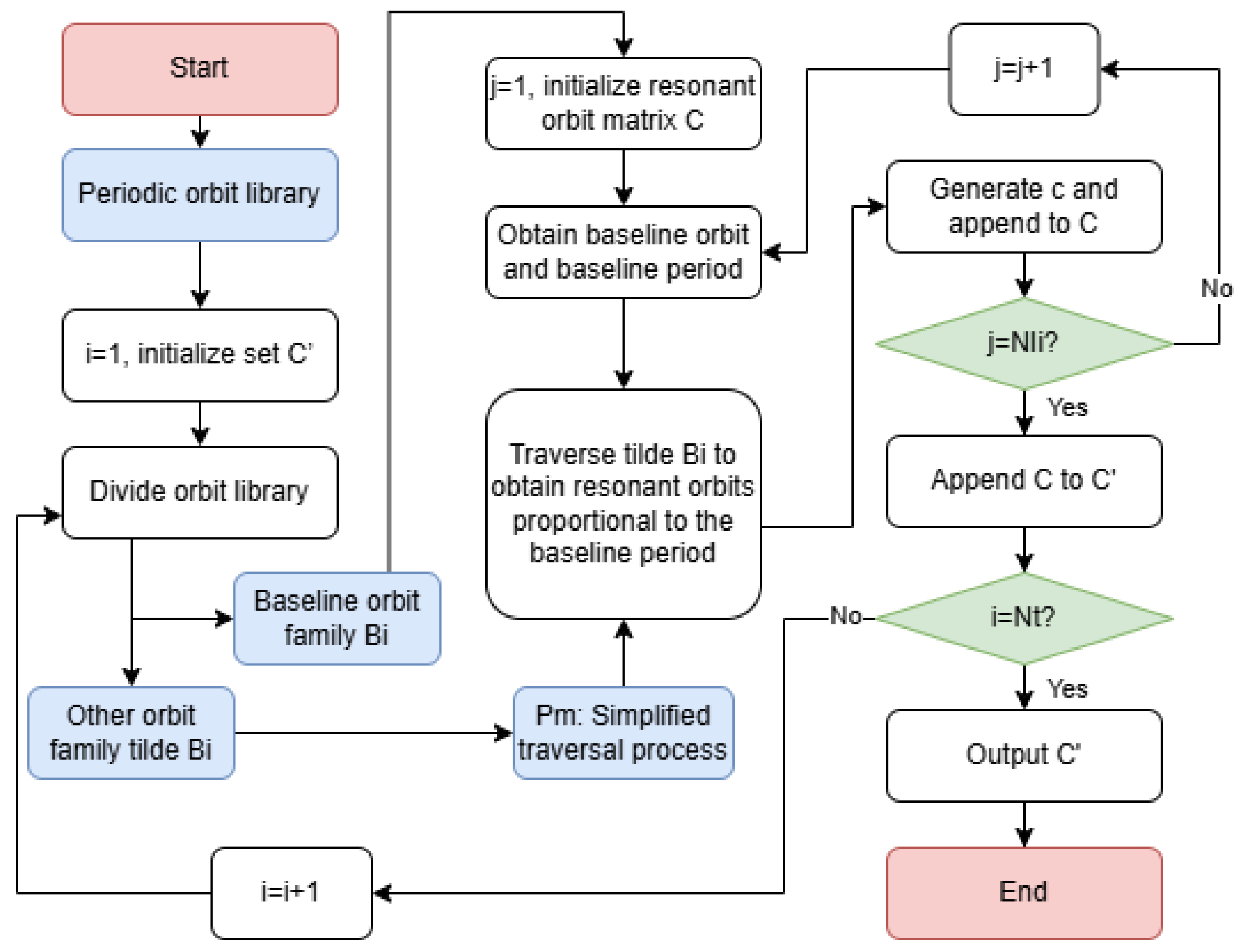
3.2. Resonant Combination Generation and Merging

The generation of resonant constellations fundamentally requires two steps: (1) selecting a reference orbit and (2) determining whether orbits from other orbital families exhibit periods that form integer ratios with the reference orbit’s period. The flowchart of the resonant combination generation algorithm is shown in Figure 4.

The corresponding orbital family ${\mathit{B}}_{I_i}$ is retrieved using its orbital type identifier $I_i$. Then, ${\tilde{\mathit{B}}}_{I_i}$ is defined as the set of all orbital families excluding ${\mathit{B}}_{I_i}$:

$${\tilde{\mathit{B}}}_{I_i}=\left\{{\mathit{B}}_{I_1},{\mathit{B}}_{I_2},\dots ,{\mathit{B}}_{I_{i-1}},{\mathit{B}}_{I_{i+1}},\dots ,{\mathit{B}}_{I_{N_t}}\right\}$$

(17)

Special boundary conditions apply when $i=1$ (first entry) or $i=N_t$ (last entry).

$${\tilde{\mathit{B}}}_{I_1}=\left\{{\mathit{B}}_{I_2},{\mathit{B}}_{I_3},\dots ,{\mathit{B}}_{I_{N_t}}\right\}$$

(18)

$${\tilde{\mathit{B}}}_{I_{N_t}}=\left\{{\mathit{B}}_{I_1},{\mathit{B}}_{I_2},\dots ,{\mathit{B}}_{I_{N_t-1}}\right\}$$

(19)

The row vector ${\tilde{\mathit{p}}}_i$ is removed from $\tilde{\mathit{P}}$ to obtain the characteristic period matrix ${\tilde{\mathit{P}}}^{\prime }$ of the remaining orbital families. The current orbital family ${\mathit{B}}_{I_i}$ is iterated through each row (orbit) indexed by $j=1,2,\dots ,N_{I_i}$, where $N_{I_i}$ denotes the row count of ${\mathit{B}}_{I_i}$ (equivalent to the total number of orbits in this family). The j-th orbit is denoted as ${\mathit{b}}_j$. The period of orbit ${\mathit{b}}_j$ is considered the reference period $p_0$. To identify all resonant orbits with periods proportional to $p_0$, the following variables are initialized:

• Resonance multiple f.
• Period ratio vector $\mathit{p}$ (storing periods proportional to $p_0$).
• Orbit combination matrix $\mathit{C}$ (recording parameters and type identifiers of resonant orbits). Each row vector $\mathit{c}$ in $\mathit{C}$ represents a resonant orbit.

$$\mathit{c}=\left[\begin{array}{cccccccc}{x}_0& y_0& z_0& {\dot{x}}_0& {\dot{y}}_0& {\dot{z}}_0& p& o\end{array}\right]$$

(20)

where o denotes the type index of the orbit.

The procedure for searching all resonant orbits associated with the current baseline orbit is as follows:

• Initialize the resonance multiple by setting $f=1$. Initialize the period ratio vector $\mathit{p}$, with its first element as $p_0$. Initialize the orbital combination matrix $\mathit{C}$. Let m represent the row index of $\mathit{C}$. When $m=1$, the first row vector records the baseline orbit; then, ${\mathit{c}}_1=\left[\begin{array}{cc}{\mathit{b}}_j& I_i\end{array}\right]$.
• Extract the last element $p_f$ from the period ratio vector $\mathit{p}$ and compare it with the maximum period $P_m$ in the working orbit library. If $p_f<P_m$, increment the resonance multiple f by 1 and append a new element $\mathit{p}=f\times p_0$ to $\mathit{p}$.
• Repeat 2 until $p_f>P_m$. Remove the last element $p_f$ from $\mathit{p}$, thereby obtaining all resonant periods in ${\tilde{\mathit{B}}}_{I_i}$ that are proportional to $p_0$, and record them in the vector $\mathit{p}$.
• To search for all resonant orbits, iterate through ${\tilde{\mathit{B}}}_{I_i}$. Denote the orbit family index within $s=1$.
• Retrieve the current orbit family ${\mathit{B}}_s$. Extract the period column vector ${\mathit{P}}_s$ from the last column of ${\mathit{B}}_s$. From ${\tilde{P}}^{\prime }$, obtain the s-th row vector ${\tilde{p}}_s$, which represents the characteristic period vector of the current orbit family.
• Iterate through $\mathit{p}$. Let the resonance period index be $k=1$, such that the current resonance period is $p_k$.
• Determine if $p_k$ lies within the range specified by ${\tilde{\mathit{p}}}_s$. If ${\tilde{p}}_{i1}<p_k<{\tilde{p}}_{i2}$ is not satisfied, $p_k$ cannot be found in the s-th orbit family. Proceed by incrementing s ($s=s+1$) and jump to 5 to iterate through the next orbit family until $s=N_t$; then, proceed to 8. If ${\tilde{p}}_{i1}<p_k<{\tilde{p}}_{i2}$ is satisfied, compute the period deviation vector $\delta {\mathit{P}}_s$.

  $$\delta {\mathit{P}}_s={\mathit{P}}_s-p_k$$

  (21)
  Retrieve the index $in$ of the minimum value in $\delta {\mathit{P}}_s$,

  $$in=\arg \min \left(\delta {\mathit{P}}_s\right)$$

  (22)
  Extract the corresponding row vector ${\mathit{b}}_{in}$ from ${\mathit{B}}_s$ and append it to the orbital combination matrix $\mathit{C}$ by incrementing m($m=m+1$)

  $${\mathit{c}}_m=\left[\begin{array}{cc}{\mathit{b}}_{in}& s\end{array}\right]$$

  (23)
  Increment k ($k=k+1$) to obtain the next $p_k$. Repeat 7 until k exceeds the number of elements in $\mathit{p}$. Increment s ($s=s+1$). If $s=N_t$, proceed to 8. Otherwise, return to 5 to iterate through the next orbit family.
• At this stage, the orbital combination matrix $\mathit{C}$, containing all orbits resonant with $p_0$, is obtained. Since the constructed resonant constellation in this study serves as a navigation constellation, which requires at least four satellites for positioning and navigation services, if the number of rows in $\mathit{C}$ is less than four, discard the current $\mathit{C}$. Otherwise, record the current $p_0$ and its corresponding matrix $\mathit{C}$ in the set ${\mathit{C}}^{\prime }$.

Steps 1-8 complete the search for resonant orbits corresponding to the baseline period $p_0$. Subsequently, increment j ($j=j+1$) and initiate a new search using the next ${\mathit{b}}_j$, using ${\mathit{B}}_{I_i}$ as the baseline period. Repeat until all orbits in ${\mathit{B}}_{I_i}$ are traversed. Then, increment i ($i=i+1$), and repeat Step 2 for the new ${\mathit{B}}_{I_i}$ until all orbit families in $\mathit{B}$ are fully traversed.

Upon completing the aforementioned procedures, the entire working orbit library $\mathit{B}$ yields the resonant combination set ${\mathit{C}}^{\prime }$, where all combinations are characterized by the baseline period.

$${\mathit{C}}^{\prime }=\left\{\{p_{01},{\mathit{C}}_{\mathbf{1}}\},\{p_{02},{\mathit{C}}_{\mathbf{2}}\},\dots \right\}$$

(24)

In this study, as exemplified by the working orbit library (Table 1), the algorithm-generated ${\mathit{C}}^{\prime }$ contains 20,366 elements. Each element represents a resonant combination comprising a variable number of orbits. When constraining the constellation size—for instance, only using four-satellite constellations–combinatorial principles indicate that ${\mathit{C}}^{\prime }$ can theoretically form 2,043,119 distinct four-satellite constellations, resulting in a substantial computational load. To address this, ${\mathit{C}}^{\prime }$ is classified according to specific criteria to reduce its scale.

The computational load reduction is primarily achieved through orbit-type composition-based combination merging and intra-combination deduplication. This process generates a condensed combination set $\tilde{\mathit{C}}\subseteq {\mathit{C}}^{\prime }$, formally defined as follows:

$$\tilde{\mathit{C}}=\left\{\{p_{0i{n}_1},{\mathit{C}}_{i{n}_1}\},\{p_{0i{n}_2},{\mathit{C}}_{i{n}_2}\},\dots ,\{p_{0i{n}_r},{\mathit{C}}_{i{n}_r}\}\right\}$$

(25)

where $i{n}_r\in Z^{+}$ denotes the index of the representative combination in ${\mathit{C}}^{\prime }$, and r represents the cardinality of the merged combinations. Upon completing the merging process and taking the navigation constellation constructed from the orbit library in this study as an example, the number of elements in $\tilde{\mathit{C}}$ is reduced from 20,366 to 95, and the number of four-satellite constellation combinations is drastically reduced to 36,569. Compared to the initial 2,043,119 constellation combinations, the computational scale is significantly reduced.

However, as the computational burden remains high, intra-combination orbital deduplication is implemented, with the coalescence of homogeneous orbit types being achieved through type-specific clustering. The combination $\mathit{C}$ in $\tilde{\mathit{C}}$ is replaced with $\stackrel{⌢}{\mathit{C}}$, which represents a deduplicated orbital combination. Then, this is updated to obtain the resonant orbit set ${\tilde{\mathit{C}}}^{\prime }$.

$${\tilde{\mathit{C}}}^{\prime }=\{p_{0i{n}_1},{\stackrel{⌢}{\mathit{C}}}_{\mathrm{i}{n}_1}\},\{p_{0i{n}_2},{\stackrel{⌢}{\mathit{C}}}_{\mathrm{i}{n}_2}\},\dots ,\{p_{0i{n}_{\mathrm{r}}},{\stackrel{⌢}{\mathit{C}}}_{\mathrm{i}{n}_{\mathrm{r}}}\}$$

(26)

3.3. Resonant Constellation Generation and Merging

Following the determination of constellation size $n_{sat}$, all constellations are generated via $C_{n_t}^{n_{sat}}$, i.e., $n_{sat}$ orbits are selected from the $n_t$ orbits in $\stackrel{⌢}{\mathit{C}}$. Note that the satellite counts $n_{sat}$ and the number of orbits in the combination must satisfy a specific relationship: if $n_t<n_{sat}$, the current combination $\stackrel{⌢}{\mathit{C}}$ is discared. Assume h valid combinations meet the quantity requirements. For the q-th combination ${\stackrel{⌢}{\mathit{C}}}_q$ all generated combinations are stored in matrix ${\mathit{A}}_q$, where each row of ${\mathit{A}}_q$ represents a constellation. The row vector $\mathit{a}=\left[\begin{array}{ccccc}{o}_1& o_2& \dots & o_{n_{sat}}& p_0\end{array}\right]$, termed the constellation vector, records the orbit types and baseline period corresponding to the constellation. This constructs a constellation matrix A, containing all $n_{sat}$-satellite constellations formed by the combinations ${\stackrel{⌢}{\mathit{C}}}_q$, with a total count of h.

$$\begin{array}{c}\hfill \mathit{A}={\left[\begin{array}{cccc}{\mathit{A}}_1& {\mathit{A}}_2& \dots & {\mathit{A}}_h\end{array}\right]}^T\end{array}$$

(27)

In this study, taking four-satellite constellations as an example, the above procedures generate a total of 6922 constellations. Among these, some constellations share identical orbital-type compositions but differ in their baseline periods. To further merge and reduce the computational scale, such constellations are represented by the one with the smallest baseline period, resulting in a submatrix $\stackrel{⌢}{\mathit{A}}$ of the constellation matrix $\mathit{A}$. Assuming the final merged constellations number is G, the following can be obtained:

$$\begin{array}{c}\hfill \stackrel{⌢}{\mathit{A}}\end{array}={\left[\begin{array}{cccc}{\mathit{a}}_1& {\mathit{a}}_2& \dots & {\mathit{a}}_G\end{array}\right]}^T$$

(28)

Finally, based on the baseline period in the constellation vector $a_g$, the corresponding resonant orbit combination ${\tilde{\mathit{C}}}^{\prime }$ is retrieved from the resonant orbit set $\stackrel{⌢}{\mathit{C}}$. Then, according to the orbit types specified in $a_g$, the corresponding initial orbital parameters can be extracted $\stackrel{⌢}{\mathit{C}}$, where $g = 1,2,\dots ,G$, thereby forming the constellation matrix.

$${\mathit{D}}_g={\left[\begin{array}{cccc}{\mathit{b}}_1& {\mathit{b}}_2& \dots & {\mathit{b}}_{{\mathit{n}}_{\mathit{s}\mathit{a}\mathit{t}}}\end{array}\right]}^T$$

(29)

By performing a row-wise traversal of $\stackrel{⌢}{\mathit{A}}$, a comprehensive set of all generated constellation matrices is obtained.

$$\begin{array}{c}\hfill \tilde{\mathit{D}}=\left\{\begin{array}{cccc}{\mathit{D}}_1& {\mathit{D}}_2& \dots & {\mathit{D}}_G\end{array}\right\}\end{array}$$

(30)

This completes the entire process of extracting all resonant constellations from the orbit library. Through the described algorithm, a total of 1229 resonant constellations are generated.

4. Simulation Analysis

Building upon the theoretical framework and resonant constellation design methodology discussed earlier, this study analyzes resonant configurations in three distinct regions—the near-Earth region, lunar region, and combined region—using a four-satellite constellation as an illustrative example. Additionally, taking the optimal configuration in the combined region as a case study, the spatiotemporal distribution characteristics of DOP values for the resonant constellation are systematically investigated.

4.1. Resonant Constellation Configuration Analysis for Distinct Regions

For each constellation group, orbital propagation was performed based on the constellation’s period. Assuming the period was discretized into n time points, a time sequence $\mathit{T}=t_0,t_1,\dots ,t_N$ was generated. Following the method outlined in Section 2.4, m grid points were derived, and a DOP matrix $\mathit{D}\in R^{n\times m}$ was constructed, yielding:

$$\mathit{D}={\left(d_{ij}\right)}_{n\times m}=\left[\begin{array}{cccc}{d}_{11}& d_{12}& \dots & d_{1m}\\ d_{21}& d_{22}& \dots & d_{2m}\\ \dots & \dots & \dots & \dots \\ d_{n1}& d_{n2}& \dots & d_{nm}\end{array}\right]$$

(31)

Here, $d_{ij}$ represents the DOP value at the j-th grid point during the i-th time instance. Each row of matrix $\mathit{D}$ records the instantaneous DOP values across all grid points. By computing the average DOP value for each row of $\mathit{D}$, a spatial average sequence of DOP values was obtained.

$${\mathit{D}}_{at}={\left[\begin{array}{cccc}{\overline{d}}_1& {\overline{d}}_2& \dots & {\overline{d}}_n\end{array}\right]}^T$$

(32)

Taking the average of this sequence yielded the spatiotemporal average DOP value, which served as the metric for evaluating the current constellation’s performance.

$$\overline{D}=\frac{\underset{i=1}{\overset{n}{\Sigma }}{\overline{d}}_i}{n}$$

(33)

For the 1229 constellation configurations derived in Section 3, coverage assessment and DOP value calculations were performed across different regions. A quadruple coverage constraint was imposed: constellation configurations with a fourfold coverage below 90% were discarded. This metric was derived by calculating the spatial percentage of regions with four simultaneously visible satellites at each epoch, then taking the temporal average. The remaining configurations were ranked based on $\overline{D}$ (sorted from smallest to largest), identifying optimal and suboptimal resonant navigation constellations for specific target regions.

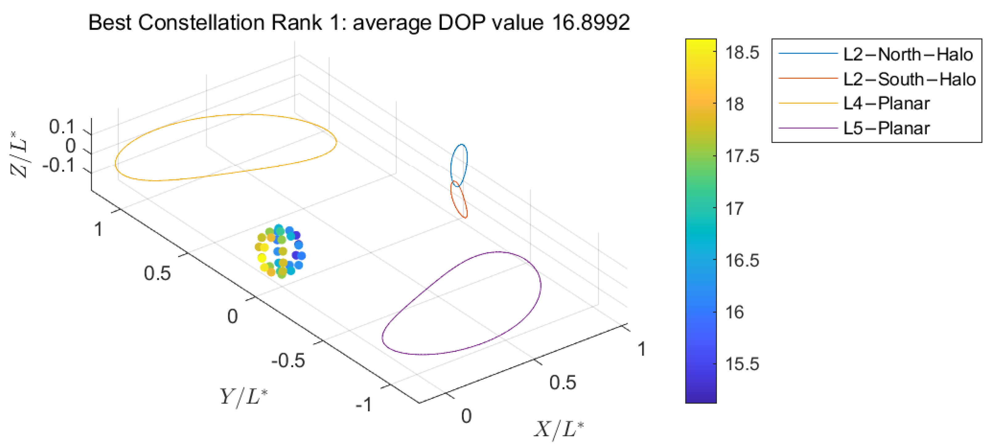
4.1.1. Near-Earth Region

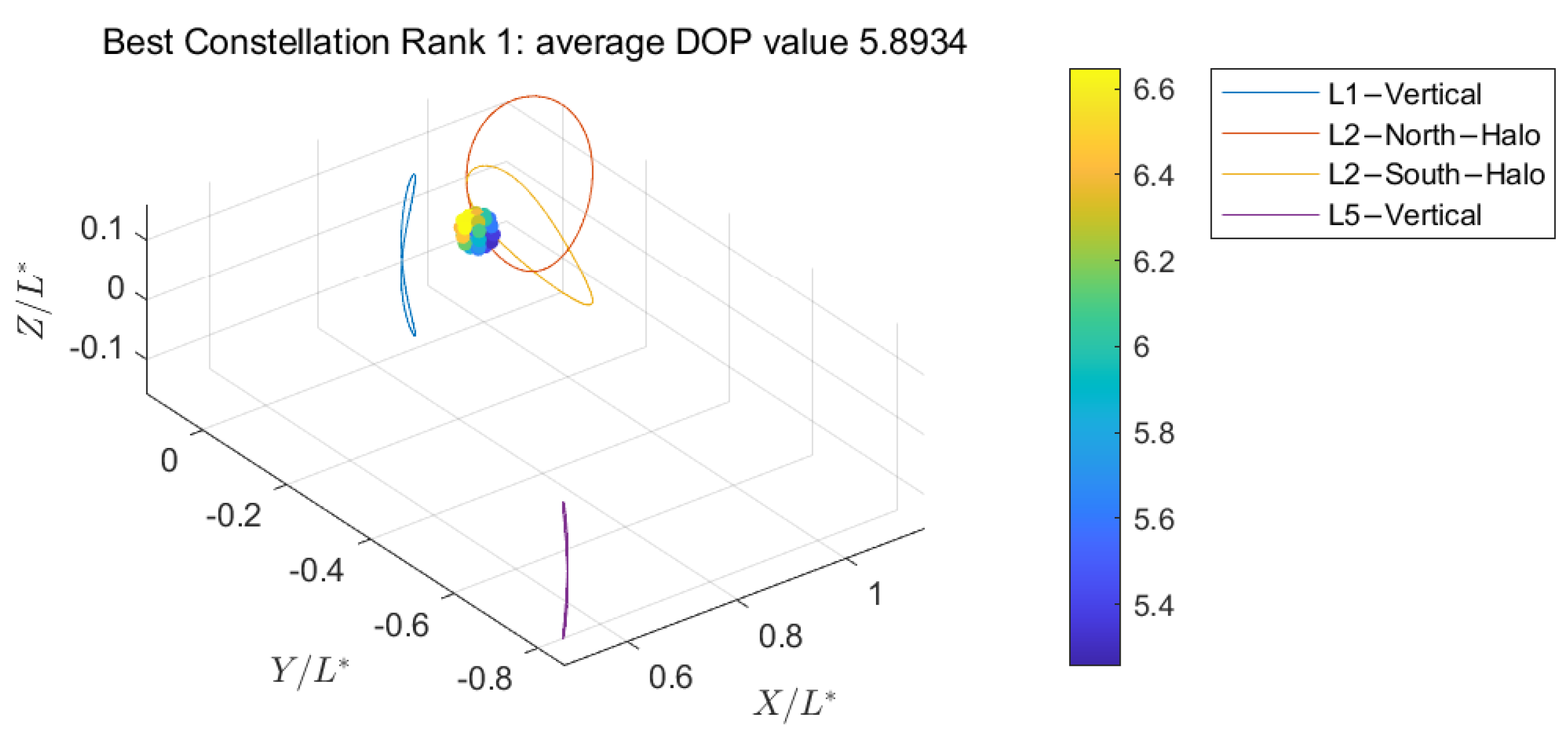
Given that high-altitude satellites in near-Earth orbits typically exhibit orbital radii of approximately 36,000 km, the simulation spherical boundary was configured at 40,000 km to ensure complete orbital encapsulation. To achieve the optimal trade-off between computational load and precision requirements, a coarse-grid discretization scheme was implemented during the preliminary screening phase. Therefore, the target region was divided into longitude intervals of 60° and latitude intervals of 30°. Applying the aforementioned algorithm, five optimal and five suboptimal constellations were identified for this region. The optimal configurations and their corresponding spatiotemporal average DOP values and standard deviations are listed in

Table 2. Dominant configurations and spatiotemporal average DOP values in the near-Earth region.

Rank	Resonant Configuration	Baseline Period	Resonance Ratio	Mean DOP	DOP SD
1	L2NH-L2SH-L4P-L5P	1.5715	1:1:4:4	16.90	3.14
2	L2NH-L2SH-L4V-L5V	1.5715	1:1:4:4	17.00	3.19
3	L1NH-L1SH-L4V-L5V	2.0947	1:1:3:3	22.01	3.98
4	L1NH-L1SH-L4P-L5P	2.1812	1:1:3:3	24.12	5.01
5	L1NH-L2SH-L5V-L4V	2.0947	1:1:3:3	22.30	21.70

. A schematic diagram of the best-performing resonant constellation configuration and the temporal average distribution of DOP values across grid points in the target region are illustrated in Figure 5.

Table 2 and Figure 5 indicate there are minimal performance differences between the Rank 1 and Rank 2 resonant constellations, with mean DOP values both below 17 and a standard deviation below 4. These two configurations incorporate L2 southern/northern NRHO orbits and periodic orbits of the same type at L4 and L5. In contrast, configurations Rank 3–Rank 5 consist of L1 or L2 southern/northern Halo orbits combined with L4/L5 periodic orbits, exhibiting mean DOP values between 22 and 25.

4.1.2. Lunar Region

The spherical simulation domain radius was configured at 10,000 km to comprehensively encapsulate the characteristic lunar orbital geometries. As in the near-Earth region, longitude and latitude intervals were set to 60° and 30°, respectively. Using the aforementioned algorithm, five optimal and five suboptimal constellations for positioning performance in this region were identified. The optimal configurations and their corresponding spatiotemporal average DOP values and standard deviations are listed in

Table 3. Dominant configurations and spatiotemporal average DOP values in the lunar region.

Rank	Resonant Configuration	Baseline Period	Resonance Ratio	Mean DOP	DOP SD
1	L1V-L2NH-L2SH-L4V	3.1417	1:1:1:2	5.89	2.07
2	L1V-L2NH-L2SH-L5V	3.1417	1:1:1:2	5.89	2.66
3	L1V-L2NH-L2SH-DRO	2.7695	1:1:1:1	10.65	4.57
4	L1V-L2NH-L1NH-L1SH	2.7695	1:1:1:1	8.46	13.80
5	L1L-L2L-L4P-L5P	3.2693	2:3:4:4	15.38	2.62

. A schematic diagram of the best-performing resonant constellation and the temporal average DOP values across grid points in the target region are illustrated in Figure 6.

Table 3 and Figure 6 demonstrate that the optimal constellation configurations for the lunar region significantly outperformed those for the near-Earth region. For instance, even the Rank 5 lunar configuration surpassed the Rank 1 near-Earth configuration, highlighting the advantage of leveraging periodic orbits for lunar navigation systems compared to geocentric ones. Furthermore, the mean DOP values for all lunar configurations were below 16, indicating high-precision navigation services for the lunar region. In terms of composition, the Rank 1 and Rank 2 configurations share similar orbital types, combining L1 vertical orbits, L2 southern/northern NRHO orbits, and L4/L5 vertical orbits.

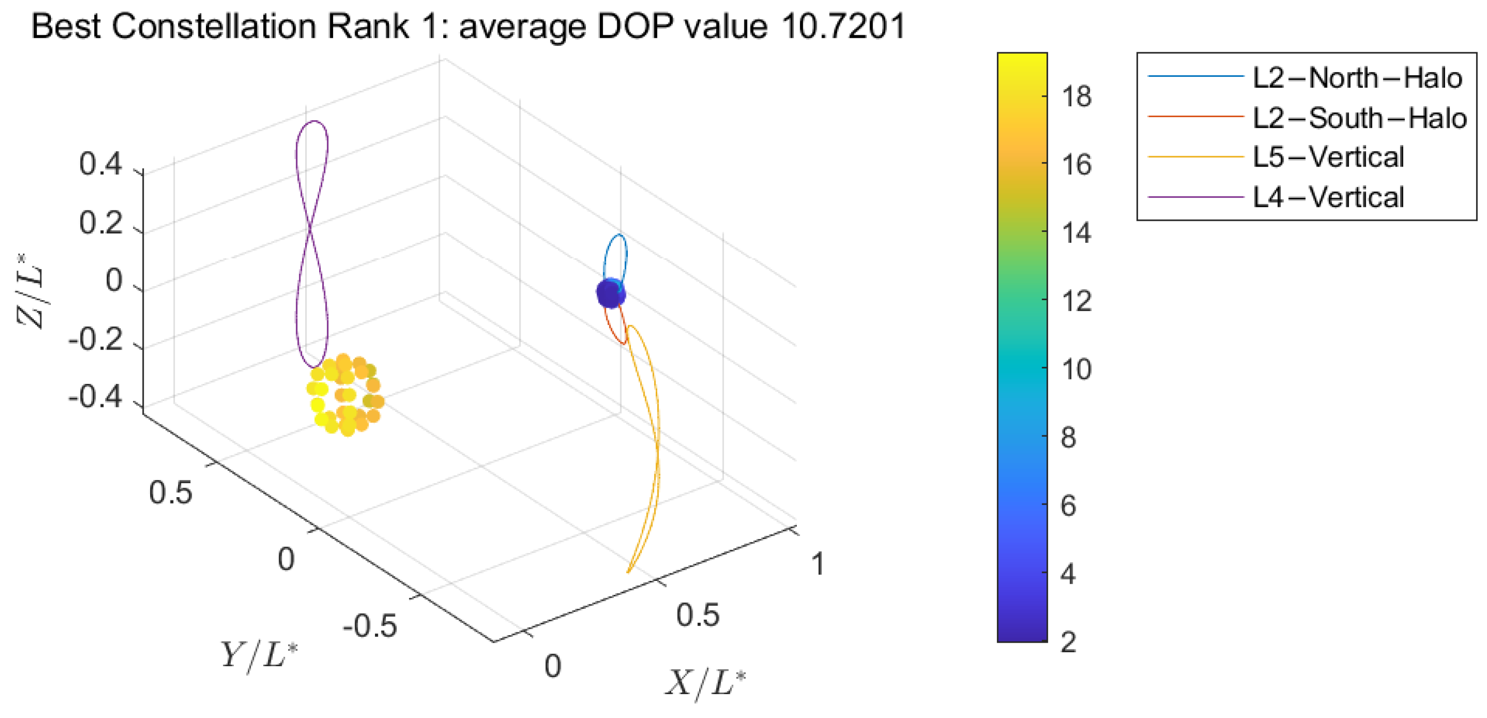
4.1.3. Combined Region

The combined region combines both the near-Earth and lunar regions as targets, with discretization parameters consistent with those defined in Section 4.1.1 and Section 4.1.2. Following the same methodology, five constellations with optimal positioning performance for this region were identified. The optimal configurations and their corresponding spatiotemporal average DOP values and standard deviations are listed in

Table 4. Dominant configurations and spatiotemporal average DOP values in the combined region.

Rank	Resonant Configuration	Baseline Period	Resonance Ratio	Mean DOP	DOP SD
1	L2NH-L2SH-L4V-L5V	1.5715	1:1:4:4	10.72	24.53
2	L2NH-L2SH-L4P-L5P	1.6352	1:1:4:4	10.86	27.70
3	L2SH-L1NH-L4V-L5V	2.0946	1:1:3:3	15.20	50.58
4	L2SH-L1NH-L4P-L5P	2.1801	1:1:3:3	16.84	92.86
5	L2NH-L1SH-L4P-L4P	2.1801	1:1:3:3	16.84	92.86

. A schematic of the best-performing resonant constellation and the temporal average DOP values across grid points in the integrated target region is illustrated in Figure 7.

The charts reveal that the Rank 1 and Rank 2 configurations for the combined region—composed of L2 southern/northern NRHO orbits and L4/L5 planar/vertical orbits—also rank as optimal configurations for both the near-Earth and lunar regions. The remaining three configurations (Rank 3–5) primarily consist of one L1 or L2 Halo orbit combined with L4/L5 orbits of the same type. Among them, Rank4 and Rank5 differ only by swapping the north–south family Halo orbit types and can thus be regarded as equivalent. An analysis of the DOP distribution indicates that the optimal configurations exhibit superior performance in the lunar vicinity.

4.2. DOP Value Distribution Analysis of Resonant Constellations

Taking the resonant constellation with optimal DOP performance in the combined region as a case study, this section investigates the spatiotemporal evolution of DOP values for both the near-Earth and lunar regions. To analyze the spatial distribution characteristics of DOP, the near-Earth region was redefined as a series of concentric multi-spherical regions with radii ranging from 10,000 km to 100,000 km. Similarly, the lunar region was redefined as concentric spheres with radii spanning 2000 km to 11,000 km, with longitude and latitude intervals refined to 10°. As established in Section 4.1.3, the optimal configuration comprises L2 southern/northern Halo orbits and L4/L5 vertical orbits, with detailed orbital parameters provided in

Table 5. Initial orbital parameters of the optimal constellation for the combined region.

Type Code	X	Y	Z	VX	VY	VZ	P
L2NH	1.026597	0	0.18507	0	−0.1130	0	1.57146
L2SH	1.026597	0	−0.1851	0	−0.1130	0	1.57146
L4V	0.509526	0.85287	0.00225	0.07968	−0.0487	0.4244	6.28584
L5V	0.508670	−0.8534	0.00225	−0.0806	−0.0467	0.4243	6.28584

.

Table 5 indicates that the constellation’s baseline period is 1.57146, with a resonant period of 6.28584, corresponding to a resonant ratio of 1:1:4:4. Orbital propagation was performed using a time step of 0.01, with numerical integration spanning one resonant period.

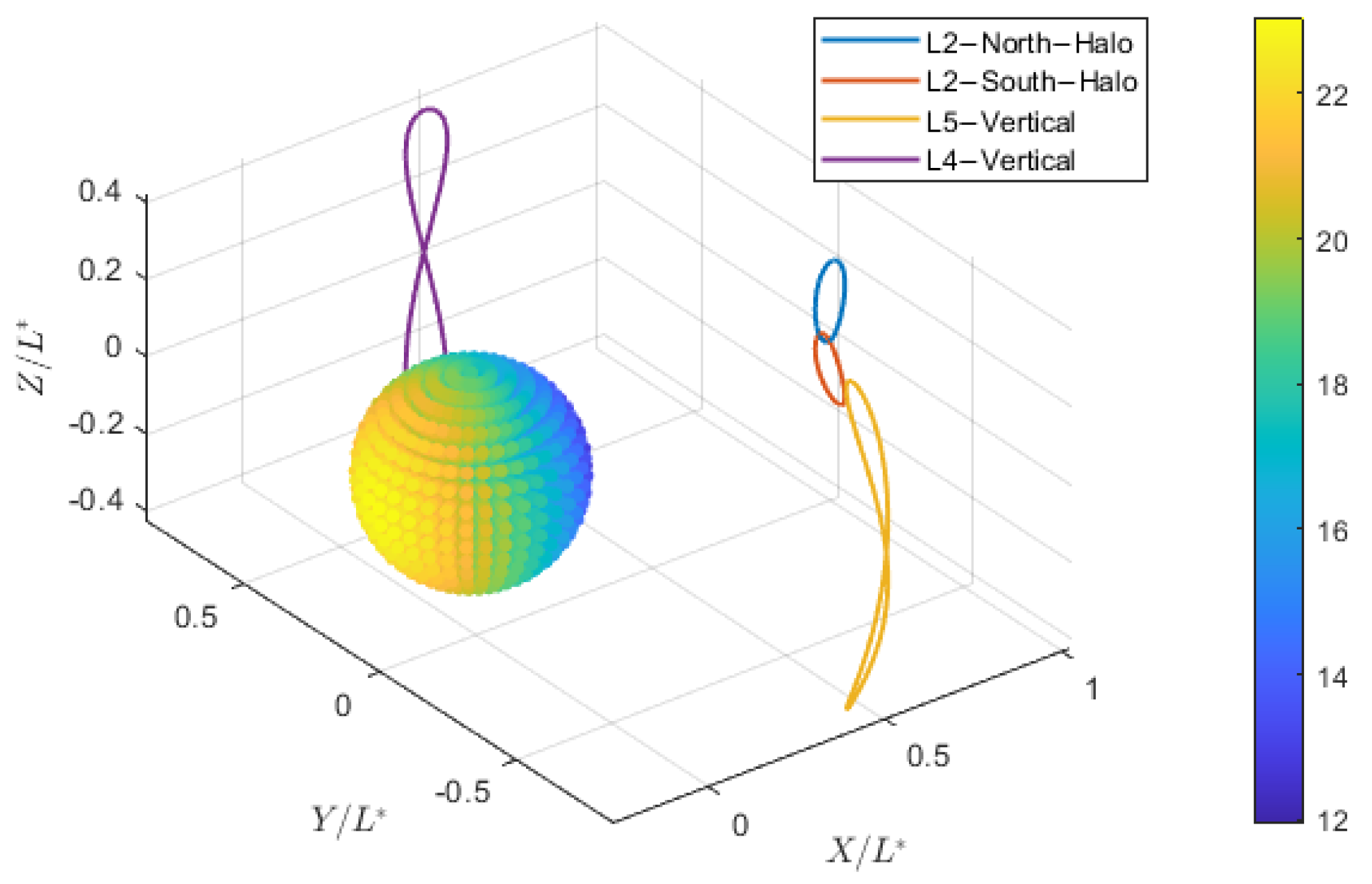
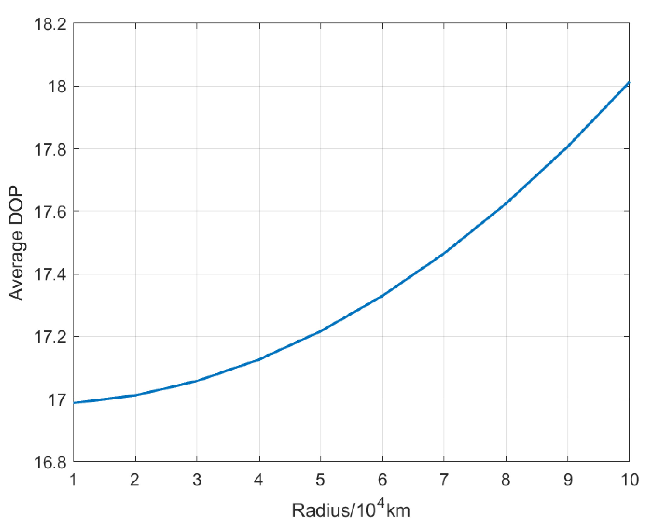
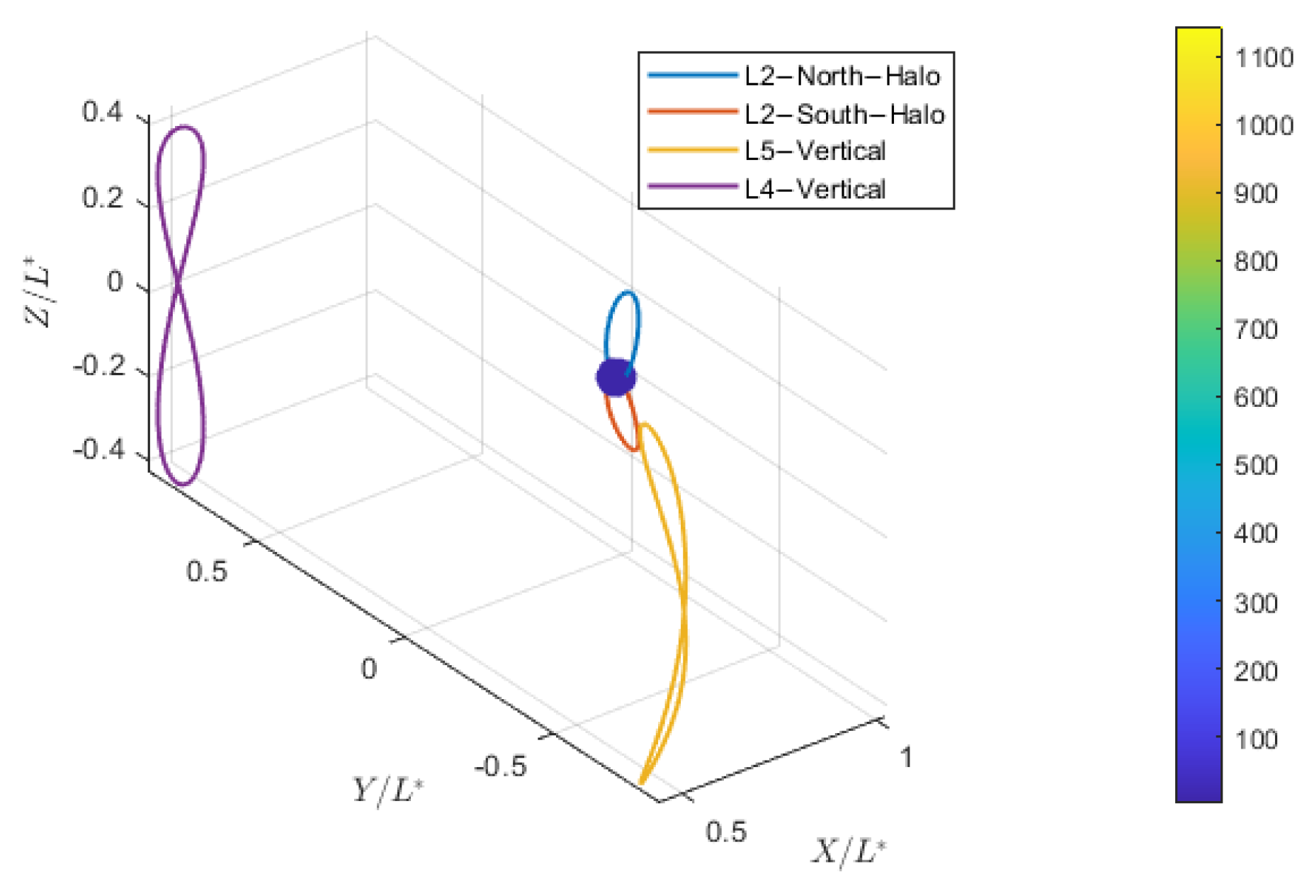
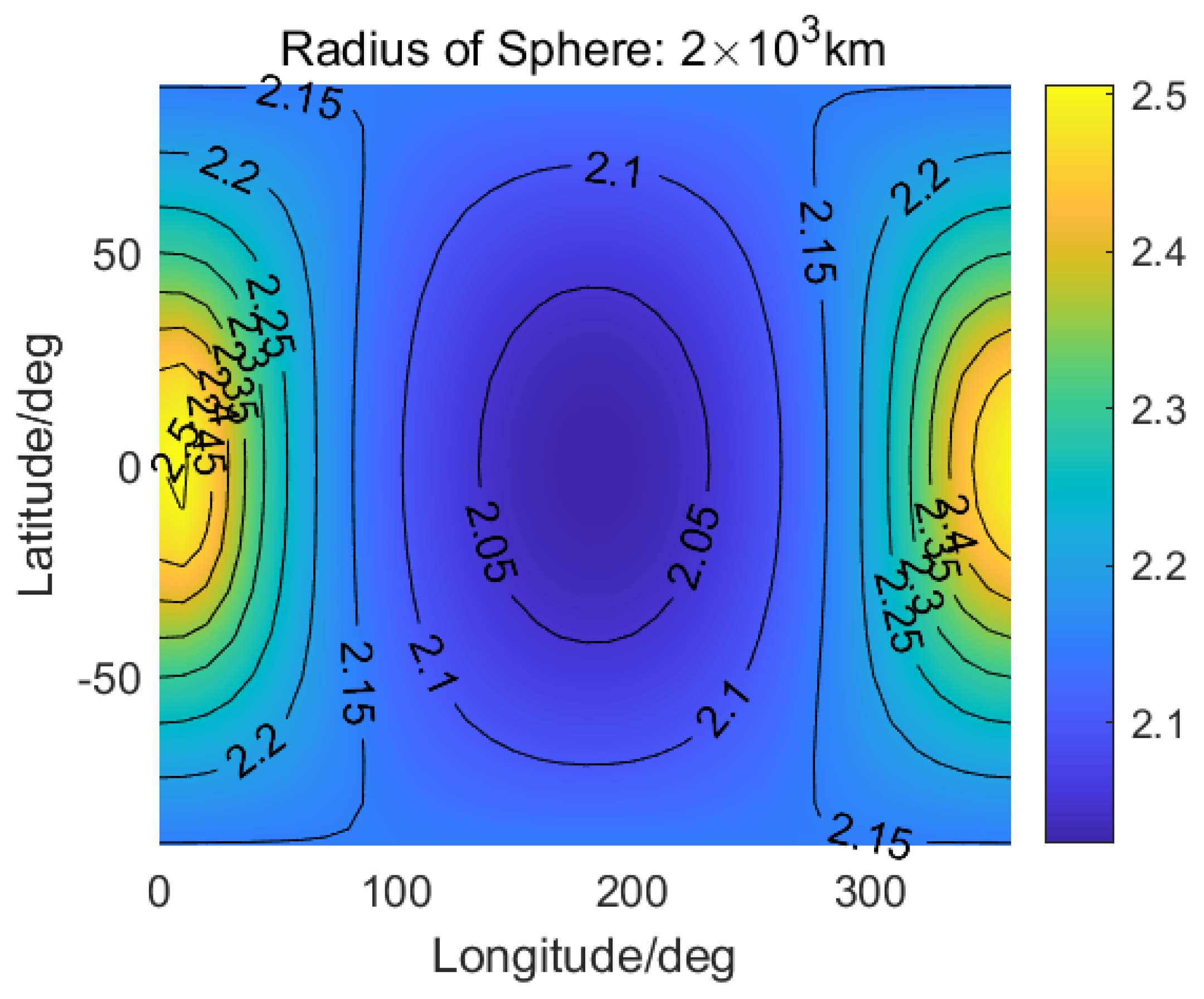
4.2.1. Performance Distribution Analysis in the Near-Earth Region

An analysis of the DOP performance in the near-Earth region yielded the constellation’s trajectory and DOP mean distribution results, as shown in Figure 8.

From a spatial perspective, the DOP temporal averages were calculated by unwrapping all target spherical surfaces to evaluate each latitude–longitude coordinate. Notably, the latitude and longitude definitions here differed from the standard geodetic coordinates:

• Longitude was defined within the Earth–Moon rotating frame, with its origin set at the intersection line of the X-Z plane and the spherical surface. This line is bisected by the spherical poles, and the longitude origin corresponds to the positive X-axis direction.
• Latitude originated from the lunar orbital plane (i.e., the “White Circle” plane), with the positive direction pointing toward the spherical north pole.

The resulting DOP distributions across the near-Earth region’s spherical surfaces are illustrated in Figure 9.

The figures reveal consistent DOP distribution patterns across all spherical layers when unwrapped. The DOP values exhibit symmetry about the Earth–Moon axis and the 0° latitude plane (the spherical equator), which is termed dual symmetry in this study. This symmetry arises because the optimal constellation is symmetric about both the Earth–Moon axis and the lunar orbital plane (White Circle plane), indicating a direct correlation between the constellation’s structural symmetry and the DOP distribution symmetry. Notably, target points within the 100°–250° longitude range exhibit higher DOP values, attributed to the constellation’s concentration near the 0° longitude side, thereby degrading the performance on the opposite side. Additionally, the DOP values decrease and their variability diminishes as the spherical radius of the target region decreases.

Further analysis of the mean DOP values for each spherical layer (plotted against radius) is presented in Figure 10. The results demonstrate a nonlinear, monotonically increasing relationship between mean DOP values and spherical radius, indicating superior service quality for low-altitude users within the near-Earth region.

4.2.2. Performance Distribution Analysis in the Lunar Region

An analysis of the DOP performance for the lunar region reveals the constellation’s trajectory and mean DOP distribution, as illustrated in Figure 11. The spherical distribution at a radius of 2000 km is shown in Figure 12.

From the figures, the 2000 km radius sphere exhibits dual symmetry characteristics, but its distribution pattern is opposite to that of the near-Earth region: the DOP values within the 100°–300° longitude range are notably lower.

Similarly, calculating the mean DOP values for each spherical layer and analyzing their relationship with the radius yields Figure 13. The results indicate that the mean DOP values generally increase with spherical radius, although anomalies occur at 4000 km, 7000 km, and 10,000 km radii. Overall, allt he mean DOP values remain below 5.5, demonstrating that this configuration provides high-precision navigation and positioning services across the entire lunar region.

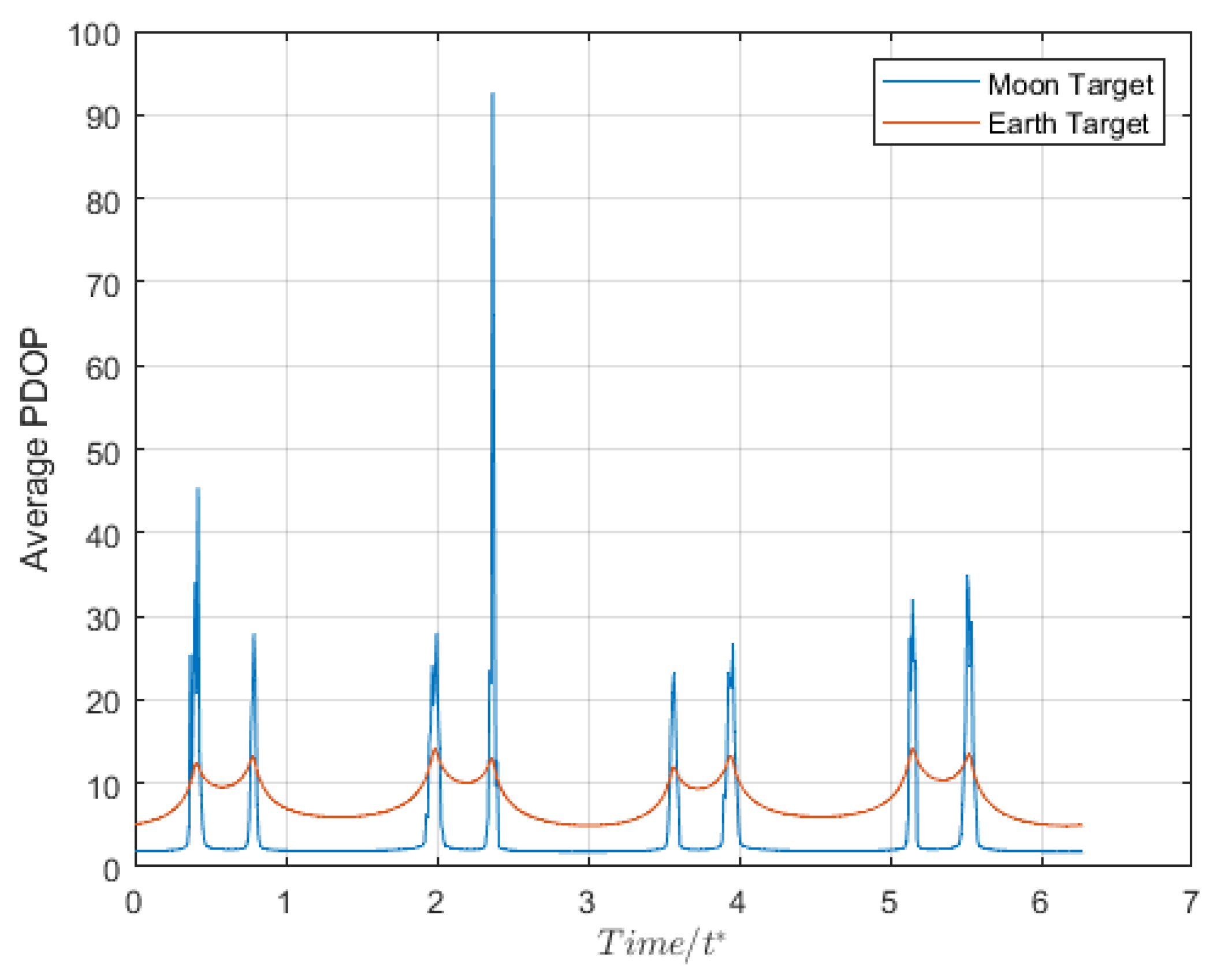
4.2.3. Time-Varying Pattern Analysis

By setting the initial phase of the baseline orbit to 90°, the DOP values are recalculated. The temporal variation curves of the spatial average DOP values in the near-Earth and lunar regions are plotted in Figure 14.

The figures show that the trends in the mean DOP values over time are consistent in both regions. Within the constellation’s resonant period, eight peaks occur, with intervals matching the baseline orbital period. The number of peaks correlates with the 1:1:4:4 resonant ratio. However, under the current initial phase, the lunar region exhibits larger peaks and more pronounced DOP fluctuations compared to the near-Earth region. Optimization methods can be applied to determine the optimal initial phase to enhance performance.

5. Conclusions

This paper proposes a cislunar resonant constellation design methodology and applies it to generate 1229 four-satellite resonant navigation constellations using a working orbit database comprising 17 orbital families. Further analyses of the constellation selection for near-Earth and lunar regions using DOP as the evaluation metric revealed the following:

• For near-Earth regions, constellations combining L2 southern/northern NRHOs with homologous periodic orbits at L4/L5 points exhibit optimal performance.
• Lunar-proximity regions achieve optimal navigation with constellations composed of L1 vertical orbits, L2 southern/northern NRHO orbits, and L4 vertical orbits.
• The combined region shares the optimal configuration with the near-Earth case.

Additionally, taking the combined region as an example, the relationship between spherical target zone radius and average DOP distribution was investigated. The results demonstrate a nonlinear monotonic increase in average DOP values with a spherical radius for near-Earth regions. For lunar regions, while the DOP values generally show an ascending trend, extremal zones emerge due to the intersections between lunar target spheres and orbital trajectories; nevertheless, the lunar DOP values remain consistently low, confirming the method’s high-precision navigation capability for lunar areas. A temporal DOP evolution analysis revealed periodic peaks aligned with baseline orbital periods, where the peak frequency correlates with resonance ratios.

References

1. Jia, Y.; Zhang, Z.; Qin, L.; Ma, T.; Lv, B.; Fu, Z.; Xue, C.; Zou, Y. Research of lunar water-ice and exploration for china’s future lunar water-ice exploration. Space Sci. Technol. 2023, 3, 0026. [Google Scholar] [CrossRef]
2. Qin, T.; Qiao, D.; Macdonald, M. Relative orbit determination using only intersatellite range measurements. J. Guid. Control Dyn. 2019, 42, 703–710. [Google Scholar] [CrossRef]
3. Hou, X.; Li, B.; Liu, X.; Cheng, H.; Shen, M.; Wang, P.; Xin, X. Initial orbit determination of some cislunar orbits based on short-arc optical observations. Astrodynamics 2024, 8, 455–469. [Google Scholar] [CrossRef]
4. Qiao, D.; Zhou, X.; Zhao, Z.; Qin, T. Asteroid approaching orbit optimization considering optical navigation observability. IEEE Trans. Aerosp. Electron. Syst. 2022, 58, 5165–5179. [Google Scholar] [CrossRef]
5. Zhou, X.; Li, X.; Huo, Z.; Meng, L.; Huang, J. Near-earth asteroid surveillance constellation in the sun-venus three-body system. Space Sci. Technol. 2022, 2022, 1–21. [Google Scholar] [CrossRef]
6. Wang, Y.; Qiao, D.; Cui, P. Analysis of two-impulse capture trajectories into halo orbits of Sun–Mars system. J. Guid. Control. Dyn. 2014, 37, 985–990. [Google Scholar] [CrossRef]
7. Qiao, D.; Jia, F.; Li, X.; Zhou, X. A review of orbital mechanics for space-based gravitational wave observatories. Space Sci. Technol. 2023, 3, 0015. [Google Scholar] [CrossRef]
8. Li, X.; Qiao, D.; Circi, C. Mars high orbit capture using manifolds in the sun–Mars system. J. Guid. Control Dyn. 2020, 43, 1383–1392. [Google Scholar] [CrossRef]
9. Li, X.; Qiao, D.; Li, P. Bounded trajectory design and self-adaptive maintenance control near non-synchronized binary systems comprised of small irregular bodies. Acta Astronaut. 2018, 152, 768–781. [Google Scholar] [CrossRef]
10. Li, C.; Liu, P.; Fu, S.; Jiao, Y.; Zhang, W. Requirement-Oriented TT&C Method for Satellite Based on BDS-3 Short-Message Communication System. Space Sci. Technol. 2023, 3, 0038. [Google Scholar]
11. Qin, T.; Macdonald, M.; Qiao, D. Fully decentralized cooperative navigation for spacecraft constellations. IEEE Trans. Aerosp. Electron. Syst. 2021, 57, 2383–2394. [Google Scholar] [CrossRef]
12. Farquhar, R.W. The Control and Use of Libration-Point Satellites; Stanford University: Stanford, CA, USA, 1969. [Google Scholar]
13. Carpenter, J.R.; Folta, D.; Moreau, M.; Quinn, D. Libration point navigation concepts supporting the vision for space exploration. In Proceedings of the AIAA/AAS Astrodynamics Specialist Conference and Exhibit, Providence, RI, USA, 16–19 August 2004; p. 4747. [Google Scholar]
14. Romagnoli, D.; Circi, C. Lissajous trajectories for lunar global positioning and communication systems. Celest. Mech. Dyn. Astron. 2010, 107, 409–425. [Google Scholar] [CrossRef]
15. Circi, C.; Romagnoli, D.; Fumenti, F. Halo orbit dynamics and properties for a lunar global positioning system design. Mon. Not. R. Astron. Soc. 2014, 442, 3511–3527. [Google Scholar] [CrossRef]
16. Xu, M.; Wang, J.; Liu, S.; Xu, S. A new constellation configuration scheme for communicating architecture in cislunar space. Math. Probl. Eng. 2013, 2013, 864950. [Google Scholar] [CrossRef]
17. Meng, Y.H.; Chen, Q.F. Outline design and performance analysis of navigation constellation near earth-moon libration point. Acta Phys. Sin. 2014, 63, 248402. [Google Scholar] [CrossRef]
18. Zhang, L.; Xu, B. A universe light house—Candidate architectures of the libration point satellite navigation system. J. Navig. 2014, 67, 737–752. [Google Scholar] [CrossRef]
19. Peng, H.; Bai, X. Natural deep space satellite constellation in the Earth-Moon elliptic system. Acta Astronaut. 2018, 153, 240–258. [Google Scholar] [CrossRef]
20. Sampaio, J.C.; Neto, A.G.S.; Fernandes, S.S.; de Moraes, R.V.; Terra, M.O. Artificial satellites orbits in 2: 1 resonance: GPS constellation. Acta Astronaut. 2012, 81, 623–634. [Google Scholar] [CrossRef]
21. Lee, H.W.; Shimizu, S.; Yoshikawa, S.; Ho, K. Satellite constellation pattern optimization for complex regional coverage. J. Spacecr. Rocket. 2020, 57, 1309–1327. [Google Scholar] [CrossRef]
22. Yin, Y.; Wang, M.; Shi, Y.; Zhang, H. Midcourse correction of Earth-Moon distant retrograde orbit transfer trajectories based on high-order state transition tensors. Astrodynamics 2023, 7, 335–349. [Google Scholar] [CrossRef]
23. Grebow, D. Generating Periodic Orbits in the Circular Restricted Three-Body Problem with Applications to Lunar South Pole Coverage. MSAA Thesis, School of Aeronautics and Astronautics, Purdue University, West Lafayette, IN, USA, 2006; pp. 8–14. [Google Scholar]
24. Vutukuri, S. Spacecraft Trajectory Design Techniques Using Resonant Orbits. Master’s Thesis, Purdue University, West Lafayette, IN, USA, 2018. [Google Scholar]
25. Jorba, A.; Masdemont, J. Dynamics in the center manifold of the collinear points of the restricted three body problem. Phys. D Nonlinear Phenom. 1999, 132, 189–213. [Google Scholar] [CrossRef]
26. Zhou, X.; Cheng, Y.; Qiao, D.; Huo, Z. An adaptive surrogate model-based fast planning for swarm safe migration along halo orbit. Acta Astronaut. 2022, 194, 309–322. [Google Scholar] [CrossRef]
27. Tang, Y.; Wu, W.; Qiao, D.; Li, X. Effect of orbital shadow at an Earth-Moon Lagrange point on relay communication mission. Sci. China Inf. Sci. 2017, 60, 1–10. [Google Scholar] [CrossRef]
28. Wang, M.; Wang, J.; Dong, D.; Meng, L.; Chen, J.; Wang, A.; Cui, H. Performance of BDS-3: Satellite visibility and dilution of precision. Gps Solut. 2019, 23, 1–14. [Google Scholar] [CrossRef]
29. Sands, O.S.; Connolly, J.W.; Welch, B.W.; Carpenter, J.R.; Ely, T.A.; Berry, K. Dilution of precision-based lunar navigation assessment for dynamic position fixing. In Proceedings of the 2006 National Technical Meeting of the Institute of Navigation, Monterey, CA, USA, 18–20 January 2006; pp. 260–268. [Google Scholar]
30. Marzullo, A. Constellation Optimization. Doctoral Dissertation, Politecnico di Torino, Torino, Italy, 2024. [Google Scholar]
31. Yarlagadda, R.; Ali, I.; Al-Dhahir, N.; Hershey, J. Gps gdop metric. IEE Proc.-Radar Sonar Navig. 2000, 147, 259–264. [Google Scholar] [CrossRef]
Figure 1. Cuboidal Spatial Gridding.
Applsci 15 04998 g001
Figure 2. Spherical Spatial Gridding.
Applsci 15 04998 g002
Figure 3. Earth–Moon resonant constellation generation methodology flowchart.
Applsci 15 04998 g003
Figure 4. The flowchart of the resonant combination generation algorithm.
Applsci 15 04998 g004
Figure 5. Schematic diagram of the optimal resonant constellation configurations and time-averaged DOP distribution in the near-Earth region.
Applsci 15 04998 g005
Figure 6. Schematic diagram of optimal resonant constellation configurations and time-averaged DOP distribution in the lunar region.
Applsci 15 04998 g006
Figure 7. Schematic diagram of optimal resonant constellation configurations and time-averaged DOP distribution in the combined region.
Applsci 15 04998 g007
Figure 8. Schematic diagram of optimal resonant constellation configurations and time-averaged DOP distribution in the combined region.
Applsci 15 04998 g008
Figure 9. Spatial distribution of DOP values in the near-Earth region. Subfigure (a) illustrates the distribution on a spherical surface with a radius of 100,000 km. Subfigure (bj) consists of a series of plots showing the DOP value distributions on spherical surfaces with radii ranging from 10,000 to 90,000 km.
Applsci 15 04998 g009
Figure 10. Variation in near-Earth region’s mean DOP value with a spherical radius.
Applsci 15 04998 g010
Figure 11. Variation in near-Earth region’s mean DOP value with a spherical radius.
Applsci 15 04998 g011
Figure 12. Variation in near-Earth region’s mean DOP value with a spherical radius.
Applsci 15 04998 g012
Figure 13. Variation in near-Earth region’s mean DOP value with a spherical radius.
Applsci 15 04998 g013
Figure 14. Variation in near-Earth region’s mean DOP value with time.
Applsci 15 04998 g014