Task-Oriented Structural Health Monitoring of Dynamically Loaded Components by Means of SLDV-Based Full-Field Mobilities and Fatigue Spectral Methods

Abstract

Expected lives of mechanical parts and structures depend upon the environmental conditions, their dynamic behaviours and the task-oriented spectra of different loadings. This paper exploits contactless full-field mobilities, estimated by Scanner Laser Doppler Vibrometry (SLDV), in the real manufacturing, assembling and loading conditions of the thin plate tested, whose structural dynamics can be described in broad frequency bands, with no distorting inertia of sensors and no numerical models. The paper derives the mobilities into full-field strain Frequency Response Functions (FRFs), which map, by selecting the proper complex-valued broad frequency band excitation spectrum, the surface strains. From the latter, by means of the constitutive model, dynamic stress distributions are computed, to be exploited in fatigue spectral methods to map the expected life of the component, according to the selected tasks’ spectra and the excitation locations. The results of this experiment-based approach are thoroughly commented in sight of non-destructive-testing, damage and failure prognosis, Structural Health Monitoring, manufacturing and maintenance actions.

1. Introduction

Any task—in which the mechanical components are used—brings its own dynamic signature, in terms of specific spectrum of loadings, the latter being external—as lumped forces or distributed pressures—or internal—as the result of motion laws or dynamics with accelerations and inertia forces. Therefore, it can be said that the specific duty a component, a mechanism or a structure, do fulfil brings a task-dependent excitation, characterised by its specific spectrum and location of energy injection. But, also, that the expected life of each mechanical part depends on both dynamic signature and location of loadings, together with the structural dynamics of the component that give responses to the specific excitation. Structural Health Monitoring (SHM) needs therefore to follow both the structural dynamics and the excitation, as they can change in time and can bring to new expected lives. In this paper, the structural dynamics is explored in one of the most adherent-to-reality approaches that is currently available, especially for lightweight structures, which starts from the broad frequency band optical full-field measurements. In this way, the experiment-based investigation deals exactly with the realisation of the structure, with the specific manufacturing and mounting conditions, with the materials and damping properties and broad band loading levels, while the above properties are hardly modellable in a numerical tool such as a Finite Element Model (FEM), also when properly tuned as in [1,2,3], but still with approximation residuals. Instead of running any Experimental Modal Analysis (EMA) as in [4,5] – also in its Experimental Full-Field Modal Analysis (EFFMA) extension in [3] – the experiment-based receptances – or displacement over force FRFs – are used to avoid any modal identification uncertainty or modal base truncation errors. Thus, full-field receptances – here obtained from SLDV-based mobilities, or velocity over force FRFs – retain the best description of the actual operative deformation shapes due to the structural dynamics, especially in the spatial domain, later used to derive the dynamic strains and feed the fatigue life estimations with increased spatial sampling and detail. Due to their intrinsic nature, full-field receptances may easily present different frequency-domain relations between response displacements and excitations, depending on the energy injection locations. In particular, a complex-valued representation of the structural dynamics is ideal to retain all the real characteristics of the test. To exploit such a refined structural dynamics, also the excitation needs to be of a complex-valued nature, as it easily comes from the signal processing of any force cell data in a test: a broad frequency band complete spectrum, with complex-valued parts, to retain all the complex amplitude and phase relations in the frequency range of interest, without simplifications nor assumptions. Already introduced with the aid of image-based receptances1, here the approach exploits instead the non-synchronous scanning of SLDV to maintain the following advantages, particularly relevant for the structural dynamics of lightweight components: (i) the real structural dynamics comes directly from testing, without the need of any tuning of the numerical modelling technique, e.g. FEM; (ii) the spatially dense grid of measurements overtakes the effort of finding the best location of traditional sensors, e.g. strain gauges; (iii) the measurements are contactless, without any distorting inertial contribution from attached sensors and their cabling. The expected task-oriented fatigue-life mapping, coming from SLDV-based full-field receptances, retains therefore the characteristic of the specific realisation of the component under test with good detail in a broad frequency band and spatial domain.

Among the optical—therefore contactless, not distorting because of sensors and cabling inertia—technologies, SLDV has permitted to add degrees of freedom (dofs) and discrete spatial resolution in established Noise and Vibration Harshness (NVH) approaches in broad frequency ranges, but it can be better defined as non-native full-field measurement technique, due to its scanning nature. SLDV has therefore become a reference in contactless measurements for standing vibrations, but not for transients, not sensing synchronously the whole mapping. SLDV is the full-field technology here adopted for the real-life mobility testing of the vibrating structural part, in order to asses its applicability to these extended data processing for fatigue life estimations. Instead, the techniques based on the sensing of photons across the whole sensor matrix can be called as optical native full-field measurements, or also image-based, with an even higher dofs’ density and field-wise accuracy/continuity than that of SLDV, as proved extensively in [3,13,14,15,16,17,18], especially with stroboscopic ESPI. Although the latter is limited to standing vibrations in the frequency domain, ESPI can measure extremely detailed fields with a noise floor of the order of 50 nm and a ceiling of some μm, exploiting the interference phase maps and the precision of the constant wavelength of the coherent laser light, modulated up to several kHz in stroboscopic acquisitions. While quality-wise unsurpassed, for broad frequency band measurements ESPI has heavy drawbacks: in the time consuming tests, in coherent lighting requirements, in recording size and environmental vibration insulation needs, all hardly met outside a specific research laboratory. Another native full-field approach is that of DIC with good spatial detail (generally better than SLDV, but lower than ESPI) in the time histories of displacement maps, once proper high-speed cameras are used related to the frequency band of interest, although generally more limited in the upper frequency than SLDV; transients are acquired in the time domain with ease; furthermore, the evaluation of multiple series of correlated displacements might be computationally intensive. A relevant advantage of DIC systems is certainly in their usage flexibility—thus of increasing interest also in industrial environments—as some in-situ applications have proved, as in [19,20,21,22,23].

Concise notes about the author’s experience in optical full-field measurements follow. The first hints of the TEFFMA project appeared in 20142, consolidated by more enhanced proceedings in 20153. The first works were briefly gathered in [17]; in [18], instead, extended notes on the full-field receptances’ evaluation followed; in [3] model updating exploited the full-field eigenshapes coming from the EFFMA. The quality of native (ESPI and DIC) full-field datasets—in broad frequency band dynamic testing—was underlined in [24]. Relevant achievements for rotational4 and strain FRF high resolution maps were compared in [6]. A risk index was firstly introduced in [7] to locate the areas mostly exposed to failure in a part subjected to dynamic load, while in [28] a damaged composite panel was tested in the same perspective. Recently, in [8], ESPI-based risk map variability was addressed by real-valued amplitude excitation signatures; the effect of the energy-injection location was investigated in [9]; both aspects were gathered in [10]. Although reduced—by interpolation in both spatial and frequency domains—to the more moderate resolutions of the SLDV references in the TEFFMA project, DIC-based full-field receptances were used instead in [11] for the risk index mapping. Instead, in [12] the raw datasets from DIC—with no numerical residuals due to the topology transforms and interpolations—boosted the risk index analyses; furthermore, the latter used complex-valued coloured noises for force signals, with potential randomness in the complex amplitude and phase. The contribution of full-field receptances was investigated also in vibro-acoustics5, with interest on the excitation dynamic signature and on the energy injection location. The author proved how—nowadays—full-field techniques already provide, even if not fully explored, clear improvements in EFFMA, but even more in advanced model updating, derivative calculations (rotational dofs, strains, stresses, risk index maps) and vibro-acoustics, thanks to the higher continuity and consistency of the fields in the datasets when compared to more traditional sensors. Therefore, a highly reliable experiment-based behavioural modelling of complex components—in their manufacturing and mounting state—may come from full-field optical mobilities, the latter retaining any modally dense structural dynamics and being able to deal with any dynamic signature of the excitation, under the linearity assumption.

Coupled with the proper loading spectrum, the experiment-based mapping here proposed can provide the distribution of structural responses in the whole sensed domain—therefore, on the macro-scale, with respect to the linearity condition under which the receptances were estimated. This macro-scale distribution of results might be underrated by many fatigue and crack propagation researches. The latter are, instead, traditionally focused on what happens in a specific location, therefore, on the micro-scale, starting from an assumed dynamic stress distribution (e.g., [31,32,33,34,35,36]). The knowledge, about the potentially changing full-field receptances and loading spectra during the monitoring of an ageing structure, can become the key-tools of SHM inquiries, because this knowledge keeps the macro-scale mapping of the strain-stress distribution updated, on which to evolve the fatigue life estimations. Only then, the many works about failure progression in each specific material6 can find full deployment in a complete macro-scale mapping of the damage inflicted by the whole spectrum of the retained dynamics. In this paper, the fatigue life mapping is based on the suggestions from [43,44,45] about random loading, and—more specifically—from [46,47,48,49,50] about the fatigue spectral approaches in the frequency domain. The literature contemplates many other approaches7, but they go beyond the task of this work. But, it can be clearly underlined that any other estimation procedure—rather than what here formulated for the provided examples—of component’s fatigue life, or of failure progression, can be extended, by means of full-field receptances from experimental optical techniques, from the micro-scale—in which each estimation procedure was developed—to the macro-scale detailed mapping. As introduced in [7,8,9,10,11,12] supported by ESPI and DIC technologies, and later focused in Section 3 with examples exploiting SLDV-based datasets, the mapping of fatigue life estimations is greatly affected by the loading spectra8 and energy injection points, of which SHM is expected to be aware. SHM indeed can benefit from this extended knowledge into failure changing scenarios—together with the inspections, again also provided by full-field experiment-based Non-Destructive Testing (NDT) techniques as in [28,36,80,81,82,83,84] and in footnote 9, of externally added flaws from unexpected accidents (e.g., [41,42]) or with recordings of unpredicted/excessive loading—especially in better managing the life-long maintenance, inspections and operative costs. The NDT results might be matched, as already suggested in [8], with the specific task-oriented failure maps, to assess the risk related to each revealed defect. Potentially, therefore, such an enhanced SHM should be able to take better informed decisions on the maintenance actions, or allowed running conditions, for a pristine, but also a defected, component undergoing the specific task. This paper gives some further applicability proofs for SHM of SLDV—only restrained into native references, without interpolation errors from the topology transforms—in evaluations of dynamic strains & stresses, as well as in estimations of component’s fatigue life. The latter benefit of highly accurate derivative approaches—advanced in [6]—to first obtain dynamic strains, then stresses with a constitutive material model, and later the related quantities for the fatigue spectral methods here adopted.

This paper is organised as follows. After this introduction in Section 1, the materials and methods in Section 2—enriched by Appendixes A–D—help to fully comprehend the theoretical background, which brought to the results proposed in Section 3 and further discussed in Section 4, before the conclusions in Section 5. “Abbreviations” finally gathers the nomenclature used in the manuscript without explicit explanations.

Figure 1. Schematic summary of the steps in the proposed experiment-based full-field approach to evaluate the cumulative damage by fatigue spectral methods as in Section 2.

Figure 1. Schematic summary of the steps in the proposed experiment-based full-field approach to evaluate the cumulative damage by fatigue spectral methods as in Section 2.

2. Materials and Methods

The backbone of the experiment-based approach is sketched in Figure 1, as here detailed. Specifically, in Section 2.1 the estimation of experiment-based full-field FRFs is addressed, with details on the testing set-up and data processing. Section 2.2—with the aid of the three Appendixes A–C to complete the mathematical details that could have made the text heavier for the reader—gives the tools to estimate maps of full-field strains and stresses FRFs, of Principal stresses and of the von Mises equivalent stresses. Section 2.3 deals with the modelling of excitation forces by means of a complex-valued spectrum. Section 2.4, together with Appendix D, gives the tools to implement the Dirlik’s semi-empirical fatigue spectral method.

Figure 2. Full-field optical measurement instruments set-up in front of the specimen on the anti-vibration table with shakers on the backside: the instruments in (a) with SLDV head close to the border of the table, the restrained thin plate in (b) and the 2 shakers in (c).

Figure 2. Full-field optical measurement instruments set-up in front of the specimen on the anti-vibration table with shakers on the backside: the instruments in (a) with SLDV head close to the border of the table, the restrained thin plate in (b) and the 2 shakers in (c).

2.1. Full-Field SLDV-Based Mobilities and Receptances from the TEFFMA Project

At the University of Technology in Vienna, Austria, the author led the TEFFMA fundamental research project, where SLDV was taken as the reference technology in the comparison among state-of-the-art optical native full-field approaches (ESPI and DIC), in complex structural dynamics and NVH studies. Note that the TEFFMA project has useful roots for this work in ESPI-based testing9, specifically for enhanced structural dynamics and fatigue life assessments, by means of spectral methods. During the TEFFMA project, as can be seen in Figure 2, the measurement instruments (of SLDV, high-speed DIC and stroboscopic ESPI) were at the core of the activities; the test rig was mounted in a dedicated seismic floor room, on top of an anti-vibration air-cushioning table. These activities were favoured by the technicians of the mechanical and electronic workshop for customised tools. More detailed notes on the test campaign can be found in [3,6,18,24].

The common set-up—to make the unique comparison in measurements for NVH and structural dynamics of the 3 full-field technologies in the TEFFMA project—came after careful considerations on the limits of each approach. This unique set-up required a very fine tuning of the details, which brought the different approaches to a feasible performance overlapping. The same structural dynamics revealed itself in the time domain for DIC, but in the frequency domain for ESPI and SLDV. The qualitative comparison seemed certainly promising already from each instrument software, but certainly not precisely super-imposable. To obtain quantitative comparisons in the TEFFMA project—not here of specific interest—accurate topology transforms were designed and carefully coded, in order to have all the 3 different techniques’ datasets cast on the same physical (geometry and frequency) references, as hinted in the following pictures.

2.1.1. Direct Characterisation by means of Full-Field Mobilities: a Brief Recall

The mobility matrix ${\mathit{H}}_{\mathit{v}}\left(\omega \right)$ follows the formulation for the H1 estimator—noise only in the outputs—found in [4,5]: it is estimated as the spectral relation between multi-output velocities and multi-input forces. In this full-field extension, the inputs are just 2 shakers, while thousands (2907) of responses are acquired on the whole surface of interest. The structural domain is represented by the vibrating surface S of the plate, whose q-th point has global coordinates ${\mathit{q}}_q$, while $\mathit{q}$ represents the whole-field’s coordinates of the active structural domain. Each element of the mobility matrix ${\mathit{H}}_{\mathit{v}}\left(\omega \right)$ can be expressed, in complex-valued representation, as:

$$H_{v_{qf}}\left(\omega \right)={\displaystyle \frac{{\sum }_{m=1}^N{S}_{{\dot{X}}_q{F}_f}^m\left(\omega \right)}{{\sum }_{m=1}^N{S}_{F_f{F}_f}^m\left(\omega \right)}}\in \mathbb{C}$$

(1)

where ${\dot{X}}_q$ is the output velocity at q-th dof induced by the input force $F_f$ at f-th dof, while $S_{{\dot{X}}_q{F}_f}^m\left(\omega \right)$ is the m-th cross-power spectral density between input and output, $S_{F_f{F}_f}^m\left(\omega \right)$ is the m-th auto-power spectral density of the input, evaluated in N repetitions.

The 3D receptance map ${\mathit{H}}_{\mathit{d}}(x,y,\omega )\in \mathbb{C}$ is easily obtained in the frequency domain, with i as the imaginary unit, as:

$${\mathit{H}}_{\mathit{d}}\left(\omega \right)=-i/\omega {\mathit{H}}_{\mathit{v}}\left(\omega \right)\in \mathbb{C}.$$

(2)

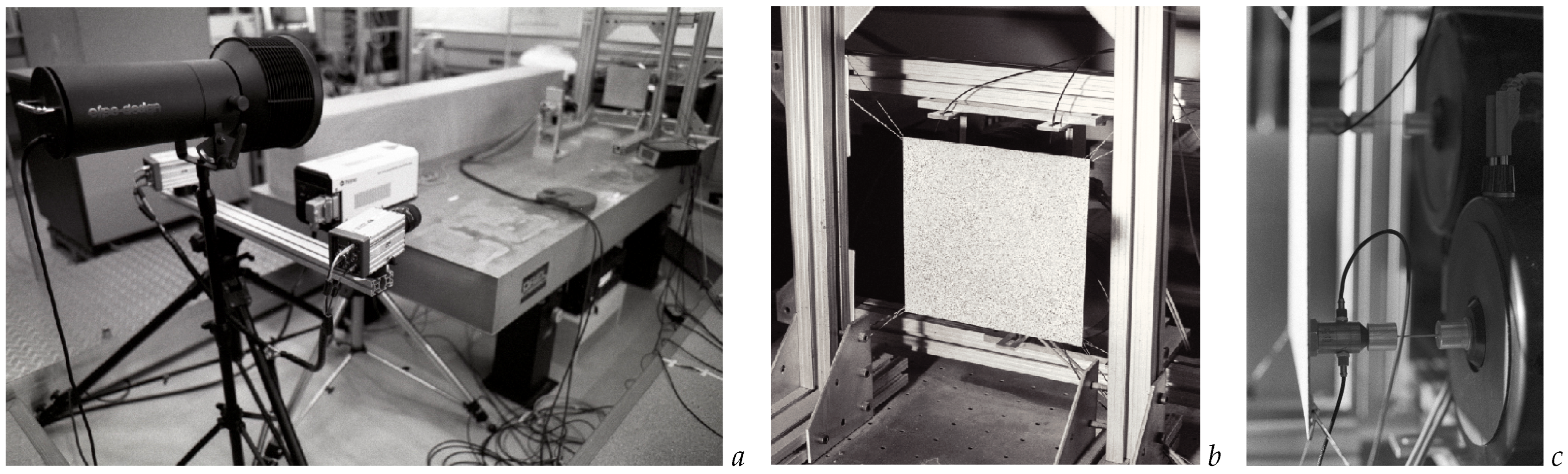
2.1.2. Notes on the Plate under Test in the TEFFMA Project

The specimen was a thin 7075-T6 aluminium alloy10 rectangular plate—flat and in pristine conditions to avoid confusion of static deformations with dynamic Operative Deflection Shapes (ODSs)—with external dimensions of 250 mm for the width, 236 mm for the height and 1.5 mm for the thickness s. It was fixed—to restrain any excessive rigid-body movement that could have impaired the ESPI technique—by wires to the rigid frame in Figure 2a,b, bolted on the air-spring optical table. A random noise patter of black & white droplets was sprayed on the face towards the instruments, accordingly to DIC requirements. Two properly positioned shakers, as in Figure 2c, excited orthogonally the plate from the back side. At each shaker-structure interface the force signal from the impedance heads was recorded for the evaluation of the mobility FRFs ${\mathit{H}}_{\mathit{v}}\left(\omega \right)$ in Equation (1). Shakers were requested by the phase-shifting procedures in ESPI-based measurements, but also fully compatible with DIC and SLDV. The shakers were driven singularly, one at a time, by an external sine-waveform generator in ESPI, instead by LMS Test.Lab system in DIC and SLDV acquisitions.

2.1.3. Processing Notes about the Estimated Full-Field Mobility FRFs

By following the formulation of Equations (1), (2), accurate mobility/receptance FRF maps were estimated from all the techniques in the TEFFMA project. It was possible to appreciate, especially for ESPI, the enhanced consistency and continuity of the spatial data—with cleans ODSs and sharp nodal lines—of the sensed structural dynamics, as also confirmed by the high-quality Coherences (see [4,5]). For each of the two shakers in different points of the structure, the SLDV-based dataset here retains $N_q$ = 2907 dofs ($N_q$ = 57 × 51, about 4.39–4.64 mm grid spacing in the structural domain, taking into account that the grid was inside the plate borders of about 2 mm, thus sized around 246 × 232 mm); each contains 1285 frequency lines, detached by a frequency space of 0.78125 Hz; the frequency range is limited to [20–1023] Hz, the lower end as imposed by ESPI technique. The number of averages is N = 50. SLDV-based datasets are here employed without any down-sampling nor interpolations due to missing topology transforms, in their raw estimation. Instead, the higher spatial resolution image-based techniques of the TEFFMA project (DIC and ESPI) are forced to contain additional computational noise from the topology transforms, if cast to the SLDV references.

2.2. Deriving New Quantities from Full-Field Receptances

Nowadays the optical full-field techniques bring high continuity and quality (see [3,17,18]) to the receptance fields, also obtainable from SLDV mobilities as in Equation (2). This allows the exploration (as from [6,8,30]) of novel derivative quantities, but limited to the plate surface. Note that, during the estimations of the TEFFMA project, only the out-of-plane-$\left(z\right)$ displacements were above the sensitivity level of all the techniques, ESPI included—albeit the most sensitive. This means that the in-plane $(x,y)$ components of the receptance map ${\mathit{H}}_{\mathit{d}}(x,y,\omega )$ were null.

2.2.1. Strain FRFs

In the case of full-field optical measurements—accurately mapping the whole spatial domain of interest with nearly-continuous data fields, but limited to the surface of the vibrating plate—the evaluation of the total strain FRF tensor ${\mathit{H}}_{\mathit{\epsilon }}(x,y,\omega )\in \mathbb{C}$ can be made, as detailed in Appendix A directly from the receptance map ${\mathit{H}}_{\mathit{d}}(x,y,\omega )$ in Equation (2), thanks to the functional relation ${\mathcal{D}}_{\epsilon }\left(\right)$ in Equation (A.4), here recalled as:

$${\mathit{H}}_{\mathit{\epsilon }}(x,y,\omega )={\mathcal{D}}_{\epsilon }\left({\mathit{H}}_{\mathit{d}}(x,y,\omega )\right)\in \mathbb{C}.$$

(3)

The diagonalisation11 of ${\mathit{H}}_{\mathit{\epsilon }}(x,y,\omega )$, made at each frequency line, further brings the complex-valued Principal Strain FRF maps ${\mathit{H}}_{\mathit{P}\mathit{\epsilon }}(x,y,\omega )$12, which retain the phase relations from the excitations, as:

$${\mathit{H}}_{\mathit{P}\mathit{\epsilon }}(x,y,\omega )=diag[{\mathit{H}}_{P_1\epsilon },{\mathit{H}}_{P_2\epsilon },{\mathit{H}}_{P_3\epsilon }](x,y,\omega )\in \mathbb{C}.$$

(4)

The experiment-based characterisation of the strain FRF distribution, over the surface of interest, turns, therefore, to be highly effective in the frequency and spatial domains.

2.2.2. Estimating the Stress FRFs

The Stress FRF tensor ${\mathit{H}}_{\mathit{\sigma }}(x,y,\omega )\in \mathbb{C}$ can be evaluated only indirectly from the total Strain FRFs in Equation (3), once a functional relation ${\mathcal{G}}_{cm}\left(\right)$ is used as the constitutive model13 of the specific material of the component. Note that the components of the Stress FRF tensor ${\mathit{H}}_{\mathit{\sigma }}(x,y,\omega )$ are expressed in [1/m²] and can be here obtained from Equation (B.2) as:

$${\mathit{H}}_{\mathit{\sigma }}(x,y,\omega )={\mathcal{G}}_{cm}\left({\mathit{H}}_{\mathit{ϵ}}(x,y,\omega )\right)={\mathcal{G}}_{cm}\left({\mathcal{D}}_{\epsilon }\left({\mathit{H}}_{\mathit{d}}(x,y,\omega )\right)\right)\in \mathbb{C}.$$

(5)

The same approach can be followed with any specific material (anisotropic and locally linearised included), by means of the deployment of the proper functional relation ${\mathcal{G}}_{cm}\left(\right)$.

Once the experiment-based Stress FRF tensor ${\mathit{H}}_{\mathit{\sigma }}(x,y,\omega )$ in Equation (5) is diagonalised, the Principal Stress FRF maps ${\mathit{H}}_{\mathit{P}\mathit{\sigma }}(x,y,\omega )$14$\in \mathbb{C}$ are obtained, therefore, from the full-field receptances ${\mathit{H}}_{\mathit{d}}(x,y,\omega )$, simply as:

$${\mathit{H}}_{\mathit{P}\mathit{\sigma }}(x,y,\omega )=diag[{\mathit{H}}_{P_1\sigma },{\mathit{H}}_{P_2\sigma },{\mathit{H}}_{P_3\sigma }](x,y,\omega )\in \mathbb{C}.$$

(6)

Figure 3. Examples of SLDV-based von Mises equivalent stress FRF maps from optical techniques in Equation (7) from shaker 1: at 121 Hz in (a), at 127 Hz in (b), at 246 Hz in (c), at 250 Hz in (d), at 279 Hz in (e), at 284 Hz in (f).

Figure 3. Examples of SLDV-based von Mises equivalent stress FRF maps from optical techniques in Equation (7) from shaker 1: at 121 Hz in (a), at 127 Hz in (b), at 246 Hz in (c), at 250 Hz in (d), at 279 Hz in (e), at 284 Hz in (f).

Figure 4. Examples of SLDV-based von Mises equivalent stress FRF maps from optical techniques in Equation (7) from shaker 1: at 333 Hz in (g), at 336 Hz in (h), at 496 Hz in (i), at 752 Hz in (l), at 755 Hz in (m), at 991 Hz in (n).

Figure 4. Examples of SLDV-based von Mises equivalent stress FRF maps from optical techniques in Equation (7) from shaker 1: at 333 Hz in (g), at 336 Hz in (h), at 496 Hz in (i), at 752 Hz in (l), at 755 Hz in (m), at 991 Hz in (n).

By following the general multi-axes von Mises Equivalent Stress15 definition, a re-arrangement of the Principal Stress FRF maps ${\mathit{H}}_{\mathit{P}\mathit{\sigma }}(x,y,\omega )$ of Equation (6), according to the functional ${\mathcal{F}}_{vM}\left(\right)$ defined in Equation (C.2), can bring the von Mises Equivalent Stress FRFs ${\mathit{H}}_{{\mathit{\sigma }}_{\mathit{vM}}}(x,y,\omega )$$\in \mathbb{C}$, which depend upon only the specific constitutive model ${\mathcal{G}}_{cm}\left(\right)$ and upon the full-field receptances ${\mathit{H}}_{\mathit{d}}(x,y,\omega )$, but remain independent from the forcing, while in linearity:

$${\mathit{H}}_{{\mathit{\sigma }}_{\mathit{vM}}}(x,y,\omega )={\mathcal{F}}_{vM}\left({\mathit{H}}_{\mathit{P}\mathit{\sigma }}(x,y,\omega )\right).$$

(7)

Examples of the von Mises Equivalent Stress FRF ${\mathit{H}}_{{\mathit{\sigma }}_{\mathit{vM}}}(x,y,\omega )$ maps in Equation (7) are given in Figures 3,4–5,6, or of single dof graphs in Figure 7, as later recalled in Section 3.1.

Figure 5. Examples of SLDV-based von Mises equivalent stress FRF maps from optical techniques in Equation (7) from shaker 2: at 121 Hz in (a), at 127 Hz in (b), at 246 Hz in (c), at 250 Hz in (d), at 279 Hz in (e), at 284 Hz in (f).

Figure 5. Examples of SLDV-based von Mises equivalent stress FRF maps from optical techniques in Equation (7) from shaker 2: at 121 Hz in (a), at 127 Hz in (b), at 246 Hz in (c), at 250 Hz in (d), at 279 Hz in (e), at 284 Hz in (f).

Figure 6. Examples of SLDV-based von Mises equivalent stress FRF maps from optical techniques in Equation (7) from shaker 2: at 333 Hz in (g), at 336 Hz in (h), at 496 Hz in (i), at 752 Hz in (l), at 755 Hz in (m), and at 991 Hz in (n).

Figure 6. Examples of SLDV-based von Mises equivalent stress FRF maps from optical techniques in Equation (7) from shaker 2: at 333 Hz in (g), at 336 Hz in (h), at 496 Hz in (i), at 752 Hz in (l), at 755 Hz in (m), and at 991 Hz in (n).

Figure 7. Examples of von Mises equivalent stress FRF graphs from SLDV optical technique in Equation (7) in 20–1023 Hz range: from shaker 1 in (a) and from shaker 2 in (b).

Figure 7. Examples of von Mises equivalent stress FRF graphs from SLDV optical technique in Equation (7) in 20–1023 Hz range: from shaker 1 in (a) and from shaker 2 in (b).

2.2.3. Estimating the Dynamic Stresses

By exploiting the complex-valued FRF formulation of the Stress FRF tensor ${\mathit{H}}_{\mathit{\sigma }}(x,y,\omega )$ as in Equation (5), (B.2), dynamic Stresses $\mathsf{\Sigma }(x,y,\omega )$$\in \mathbb{C}$ are easily computed as:

$$\mathsf{\Sigma }(x,y,\omega )={\mathit{H}}_{\mathit{\sigma }}(x,y,\omega )F\left(\omega \right)\in \mathbb{C},$$

(8)

with components as expressed in [N/m²], but where a $F\left(\omega \right)\in \mathbb{C}$ force is used, as in the general modelling of real-life excitations proposed in Section 2.3, under the linearity assumption between structural responses and excitations, grounding Equation (1).

There are two equivalent means—the diagonalisation base being the same—of obtaining the detailed maps of the dynamic Principal Stresses ${\mathsf{\Sigma }}_P(x,y,\omega )$16$\in \mathbb{C}$: (i) by the diagonalisation of the dynamic Stresses $\mathsf{\Sigma }(x,y,\omega )\in \mathbb{C}$ in Equation (8); (ii) by exploiting the FRF-based formulation of the Principal Stress FRF maps ${\mathit{H}}_{\mathit{P}\mathit{\sigma }}(x,y,\omega )$ with a proper $F\left(\omega \right)\in \mathbb{C}$ excitation. All this means:

$$\begin{array}{cc}\hfill {\mathsf{\Sigma }}_P(x,y,\omega )& =diag[{\mathsf{\Sigma }}_{P_1},{\mathsf{\Sigma }}_{P_2},{\mathsf{\Sigma }}_{P_3}](x,y,\omega )\hfill \\ \hfill & ={\mathit{H}}_{\mathit{P}\mathit{\sigma }}(x,y,\omega )F\left(\omega \right)=diag[{\mathit{H}}_{P_1\sigma },{\mathit{H}}_{P_2\sigma },{\mathit{H}}_{P_3\sigma }](x,y,\omega )F\left(\omega \right)\in \mathbb{C}.\hfill \end{array}$$

(9)

As above in the FRF formulation of Equation (7), the Principal Stresses ${\mathsf{\Sigma }}_P(x,y,\omega )$ coming from Equation (9), version (i), can be re-arranged—according to the functional ${\mathcal{F}}_{vM}\left(\right)$ defined in Equation (C.2) for general multi-axes stress definition—in the von Mises Equivalent Stress ${\mathsf{\Sigma }}_{\mathit{vM}}(x,y,\omega )\in \mathbb{C}$:

$${\mathsf{\Sigma }}_{\mathit{vM}}(x,y,\omega )={\mathcal{F}}_{vM}\left({\mathsf{\Sigma }}_{\mathit{P}}(x,y,\omega )\right)\in \mathbb{C}.$$

(10)

But here working with the Principal Stresses ${\mathsf{\Sigma }}_P(x,y,\omega )$ coming from Equation (9), version (ii), is preferred in obtaining the von Mises Equivalent Stress ${\mathsf{\Sigma }}_{\mathit{vM}}(x,y,\omega )$, because the FRF-based approach evaluates ${\mathit{H}}_{{\mathit{\sigma }}_{\mathit{vM}}}(x,y,\omega )$ only once, while varying the excitation:

$${\mathsf{\Sigma }}_{\mathit{vM}}(x,y,\omega )={\mathit{H}}_{{\mathit{\sigma }}_{\mathit{vM}}}(x,y,\omega )F\left(\omega \right)\in \mathbb{C}.$$

(11)

Albeit both Equations (10), (11) give the same result, Equation (11) is preferred in this approach, or whenever force/input shaping optimisation targets are sought, for the multiple excitations used afterwards in Section 3.

2.3. Excitation Forces: a Simple Formulation of their Spectra

Any complex-valued spectrum of the excitation $F\left(\omega \right)\in \mathbb{C}$, respecting the linearity between forces and structural responses, can be used in this approach, grounded on experiment-based full-field mobilities or receptances, which are able to retain—in the complex-valued representation—the fine details of the real-life structural dynamics. To simulate what can be generally acquired for forces in any real testing, a complex-valued coloured noise excitation is adopted, therefore with variable complex amplitude and phase in a fully populated broad frequency band, potentially with random variations on the amplitude and phase.

Figure 8. SLDV-based examples of von Mises equivalent stress PSD log-amplitude frequency domain graphs of Equation (13), from dof 550 in the 20–1023 Hz range, superimposed onto the Auto Power Spectrum of the used violet noise-rap excitation in Equation (12): from shaker 1 in (a) and from shaker 2 in (b).

Figure 8. SLDV-based examples of von Mises equivalent stress PSD log-amplitude frequency domain graphs of Equation (13), from dof 550 in the 20–1023 Hz range, superimposed onto the Auto Power Spectrum of the used violet noise-rap excitation in Equation (12): from shaker 1 in (a) and from shaker 2 in (b).

Figure 9. SLDV-based examples of von Mises equivalent stress PSD log-amplitude frequency domain graphs of Equation (13), from dof 550 in the 20–1023 Hz range, superimposed onto the Auto Power Spectrum of the used blue noise-rap excitation in Equation (12): from shaker 1 in (a) and from shaker 2 in (b).

Figure 9. SLDV-based examples of von Mises equivalent stress PSD log-amplitude frequency domain graphs of Equation (13), from dof 550 in the 20–1023 Hz range, superimposed onto the Auto Power Spectrum of the used blue noise-rap excitation in Equation (12): from shaker 1 in (a) and from shaker 2 in (b).

Complex-Valued Coloured Noise with Random Amplitude and Phase Variations

A general formulation for broad frequency band signals is here proposed for the sake of exemplification: the complex amplitude modulation of the excitation spectrum depends on the type of the coloured noise adopted, while the complex phase is imposed by a specific function. The parameter $\alpha \in [-2,2]$ defines the noise colour: $\alpha =-2$ for violet noise as in Figure 8, $\alpha =-1$ for blue noise as in Figure 9, $\alpha =0$ for white noise (here not pictured), $\alpha =1$ for pink noise as in Figure 10 and $\alpha =2$ for red noise as in Figure 11. Randomness is added in both the components of the spectrum. Therefore, the signal $F\left(\omega \right)$, receiving the ending label of "rap" (for the random variations in the modulated amplitude and sinusoidal phase), can be defined as:

$$F\left(\omega \right)={\displaystyle \frac{F_{0_r}}{{\omega }^{\alpha }}}{e}^{i{\theta }_r\left(\omega \right)}\in \mathbb{C},$$

(12)

with $F_{0_r}=F_0(1+{\beta }_{F_0}(Ran{d}_{F_0}-0.5))$, ${\theta }_r\left(\omega \right)=\theta \left(\omega \right)(1+{\beta }_{\theta }(Ran{d}_{\theta }-0.5))$ with $\theta \left(\omega \right)$ as the chosen phase function, contaminated by amplitude and phase random variations. In this general formulation, the following quantities are defined: $F_0\in \mathbb{R}$ is the reference amplitude; ${\beta }_{F_0}\in \mathbb{R}$, being $0\le {\beta }_{F_0}\le 1$, is the level of randomness in the amplitude; $Ran{d}_{F_0}$, or $Ran{d}_{\theta }$, is a function returning a pseudo-random number in the range 0 to 1, respectively for the amplitudes or for the phases; $\theta \left(\omega \right)=S_{0}sin(\pi N_p(\omega -{\omega }_0)/\Delta \omega +{\theta }_0)$ is a selected phase function; ${\beta }_{\theta }$ is the level of randomness in the phase; $S_0\in \mathbb{R}$ is the sinusoidal phase range multiplier; $N_p$ is the number of half cycles of the phase in the range; ${\omega }_0$ is the starting frequency; $\Delta \omega$ is the frequency range; ${\theta }_0$ is a reference phase. For all the examples provided in Section 3, the above mentioned quantities take these values: $F_0=0.080$ N, ${\beta }_{F_0}=0.15$, $S_0=0.5$ rad, ${\beta }_{\theta }=0.5$, $N_p=5.5$, ${\theta }_0=\pi /2$ rad.

Figure 10. SLDV-based examples of von Mises equivalent stress PSD log-amplitude frequency domain graphs of Equation (13), from dof 550 in the 20–1023 Hz range, superimposed onto the Auto Power Spectrum of the used pink noise-rap excitation in Equation (12): from shaker 1 in (a) and from shaker 2 in (b).

Figure 10. SLDV-based examples of von Mises equivalent stress PSD log-amplitude frequency domain graphs of Equation (13), from dof 550 in the 20–1023 Hz range, superimposed onto the Auto Power Spectrum of the used pink noise-rap excitation in Equation (12): from shaker 1 in (a) and from shaker 2 in (b).

Figure 11. SLDV-based examples of von Mises equivalent stress PSD log-amplitude frequency domain graphs of Equation (13), from dof 550 in the 20–1023 Hz range, superimposed onto the Auto Power Spectrum of the used red noise-rap excitation in Equation (12): from shaker 1 in (a) and from shaker 2 in (b).

Figure 11. SLDV-based examples of von Mises equivalent stress PSD log-amplitude frequency domain graphs of Equation (13), from dof 550 in the 20–1023 Hz range, superimposed onto the Auto Power Spectrum of the used red noise-rap excitation in Equation (12): from shaker 1 in (a) and from shaker 2 in (b).

2.4. Spectral Methods for Cumulative Damage and Fatigue Life Assessment in Brief

The equivalent range of stress cycles $S_{eq}$ is targeted by any spectral method for fatigue life estimation, because $S_{eq}$ represents the cumulative damage inferred by the known excitation spectrum on the specific component, due to its involved structural dynamics. The experiment-based Stress FRF maps ${\mathit{H}}_{\mathit{\sigma }}(x,y,\omega )$ in Equation (5) and the selected complex-valued spectrum of $F\left(\omega \right)$ offer unprecedented abilities in mapping, in each location $(x,y)$ of the sensed surface, the equivalent range of stress cycles $S_{eq}(x,y)$, by means of a full-field extension of the fatigue spectral methods.

Many spectral methods (e.g., [46,47,48,49,50,88,89,90,91,92,93,94,95,96,97,98]) are based on punctual evaluations, in each location $(x,y)$ of the spatial domain, of $m_k(x,y)={\int }_0^{\infty }{f}^{k}PS{D}_{{\mathrm{\Sigma }}_{vM}}(x,y,\omega )d\omega$, the k-th order moments of the frequency by ${PSD}_{{\mathrm{\Sigma }}_{vM}}(x,y,\omega )$, the Power Spectral Density (PSD) of von Mises Equivalent Stress, from which we can obtain other parameters, such as the effective frequency $F_{zerocrossing}(x,y)=F_{zc}(x,y)=\sqrt{m_2(x,y)/m_0(x,y)}$, the expected number of peaks per unit time $F_{peaks}(x,y)=F_p(x,y)=\sqrt{m_4(x,y)/m_2(x,y)}$, and the irregularity factor $\gamma (x,y)={\gamma }_2(x,y)=F_{zc}(x,y)/F_p(x,y)=m_2(x,y)/\sqrt{m_0(x,y)m_4(x,y)}$.

The ${PSD}_{{\mathrm{\Sigma }}_{vM}}(x,y,\omega )$ map can be computed, from the statements for the von Mises Equivalent Stress ${\mathsf{\Sigma }}_{\mathit{vM}}(x,y,\omega )\in \mathbb{C}$ in Section 2.2.3 and Equation (11), as:

$$PS{D}_{{\mathrm{\Sigma }}_{vM}}(x,y,\omega )=2{\mathsf{\Sigma }}_{\mathit{vM}}(x,y,\omega ){\mathsf{\Sigma }}_{\mathit{vM}}^{*}(x,y,\omega )/\Delta \omega \in \mathbb{R},$$

(13)

where ${\left(\right)}^{*}$ is the complex conjugate operator, $\Delta \omega$ is the frequency domain spectral spacing, and the multiplier 2 is for counting only the positive frequencies in a symmetric domain.

As anticipated above, when adopting varying complex-valued coloured noises for $F\left(\omega \right)$, the here preferred formulation for evaluating the PSD maps of von Mises Equivalent Stress is that in Equation (11), exploiting itself the von Mises Equivalent Stress FRFs ${\mathit{H}}_{{\mathit{\sigma }}_{\mathit{vM}}}(x,y,\omega )\in \mathbb{C}$ of Equation (7). For the sake of exemplifications, the latter ${\mathit{H}}_{{\mathit{\sigma }}_{\mathit{vM}}}(x,y,\omega )$ were shown, from both shakers, in the selected maps of the tiles—at single frequencies—in Figures 3,4–5,6, and in the whole frequency domain graphs of Figure 7, in the single dof 550. Note that any other17 spectral method, than what here simulated, can exploit the proposed experiment-based full-field approach. Specifically, all the spectral methods taking advantages from true complex-valued amplitude and phase relations—without the limiting multi-axes von Mises Stress equivalence—are expected to reach new achievements by means of the experiment-based full-field Stress FRFs ${\mathit{H}}_{\mathit{\sigma }}(x,y,\omega )$ in Equation (5), by the related principal FRF components ${\mathit{H}}_{\mathit{P}\mathit{\sigma }}(x,y,\omega )$ in Equation (6), or by the dynamic Stresses $\mathsf{\Sigma }(x,y,\omega )$ of Equation (8) with their principal components ${\mathsf{\Sigma }}_{\mathit{P}}(x,y,\omega )$ in Equation (9).

Once a specific fatigue spectral method18 is adopted to evaluate $S_{eq}(x,y)$, it is possible to calculate the Time-to-Failure spatial distribution $T_{failure}(x,y)$ ([s] or [h]), or its reciprocal Frequency-to-Failure spatial distribution $F_{failure}(x,y)$ ([1/s] or [1/h]), evaluated across all the dofs $(x,y)$ of the maps, function of $S_{eq}(x,y)$, of $F_p(x,y)$ and of the $K_r$ fatigue strength coefficient and b exponent19, as:

$$T_{failure}(x,y)=K_r/\left[F_p(x,y)S_{eq}^b(x,y)\right],$$

(14)

$$F_{failure}(x,y)=\left[F_p(x,y)S_{eq}^b(x,y)\right]/K_r.$$

(15)

3. Results

This section gives numerical examples of achievements obtainable from the proposed experiment-based full-field approach in Section 2. Section 3.1 recalls the numerical derivative evaluations of the von Mises Equivalent Stress FRFs. In Section 3.2 different PSDs of von Mises Equivalent Stress are recalled, by changing the amplitude modulation with the coloured noise model and by choosing the energy injection point, thus the underneath experiment-based structural dynamics. The same excitations are further used, with the aid of Dirlik’s fatigue spectral method, to simulate the expected distributions of Time-to-Failure in Section 3.3 and maps of Frequency-to-Failure in Section 3.4.

Some notes on the proposed maps of the figures follow to help the reader in better understanding the information they provide. First, the top-line text describes briefly the sketched function, followed by the indication of the active (in dark yellow text) and mute (in dark grey text) shakers, with corresponding structural dofs, also reported on the map by a big dot. For SLDV datasets, shaker 1 was in dof 2611, shaker 2 in dof 931. All the maps are 3D complex-valued fields, but projected with the same geometrical view and phasing angle to keep the comparison viable. Therefore, the third text line says which complex-valued part is figured, while the fourth line gives the projecting phase angle. While the $(x,y)$ coordinates correspond to those of the measurement points of the SLDV acquisitions, the $\left(z\right)$ ordinate expresses the value reached by the sketched function in the specific dof. Moreover, blue tones are associated to the $\left(z\right)$ ordinate, giving brightest blue (rgb=[0,0,1]) to the maximal value of the function in the range, while giving darkest blue (rgb=[0,0,0], or pure black) to the lowest value in the range. Also the triangles of the maps, rendered by OpenGL primitives, are coloured accordingly with the colours of the defining $(x,y,z)$ points. It may happen that the OpenGL back-face culling cuts the added big dots in some geometrical 3D views, whereas the top views present no issues. The ranges of the sketched function are drawn at the left side of each map, with the linearly varying blue tones and the extremes of the whole range. On each map, an inquiry dof is highlighted by a magenta big dot; its number (here 550) is written in the magenta text (fifth line) above the map; the value of the function reached in the inquiry dof is reported in blue in the sixth text line, but also by a magenta dash in the side ranges.

Some notes also about all the 2D frequency domain graphs is here given. At the top of each figure, generally three lines of coloured text are annotated. The first contains, on the left side, the frequency step and corresponding value in Hertz, in dark yellow, corresponding to the vertical line in the graph, or cursor; at the centre, in magenta, the dof of inquiry is proposed before the name of the main function of the graph. The second line, on the right side, shows in blue the value of the main function at the cursor’s abscissa, with related bracketed quantities; eventually, in the case of complex amplitude and phase, this information is split also to the third line. The third line can be instead taken, when only the amplitude of the functions is shown, by the description of the eventually added function and value at the cursor position, in black with left margin. The sketched functions, or complex-valued parts, are framed by grey lines, with the main functions’ extremes and bracketed dimensions on the right side in grey text, while the frequency range is annotated in grey text at the very bottom of the frame. Another text line, at the very bottom, indicates the geometrical and frequency references (here both reporting SLDV), together with the used shaker in the specific structural dof, marking it with dark yellow, whereas the mute shaker is in dark grey. Inside the frame, the main function is drawn in pure blue, and the measurement technology (here SLDV) is reminded in blue text at the right of the frame. The dark yellow vertical cursor intercepts the main function in a point through which an horizontal blue line is added to show the reached main function value. If another function is superimposed—with its own ordinate quantities, scales and ranges annotated on the right of the frame—the colour of choice is pure black, but the value at the cursor position is only reported in the text above.

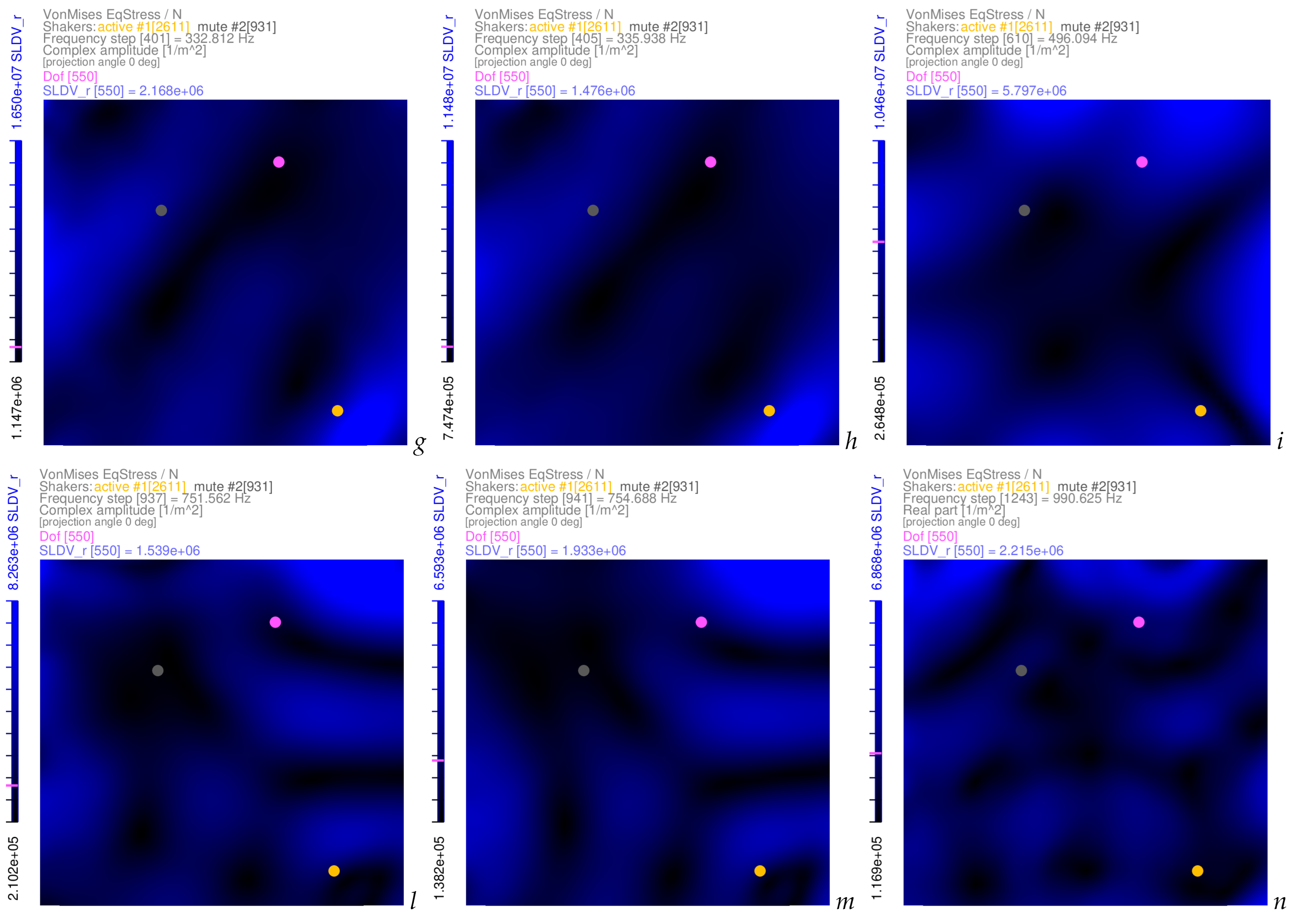
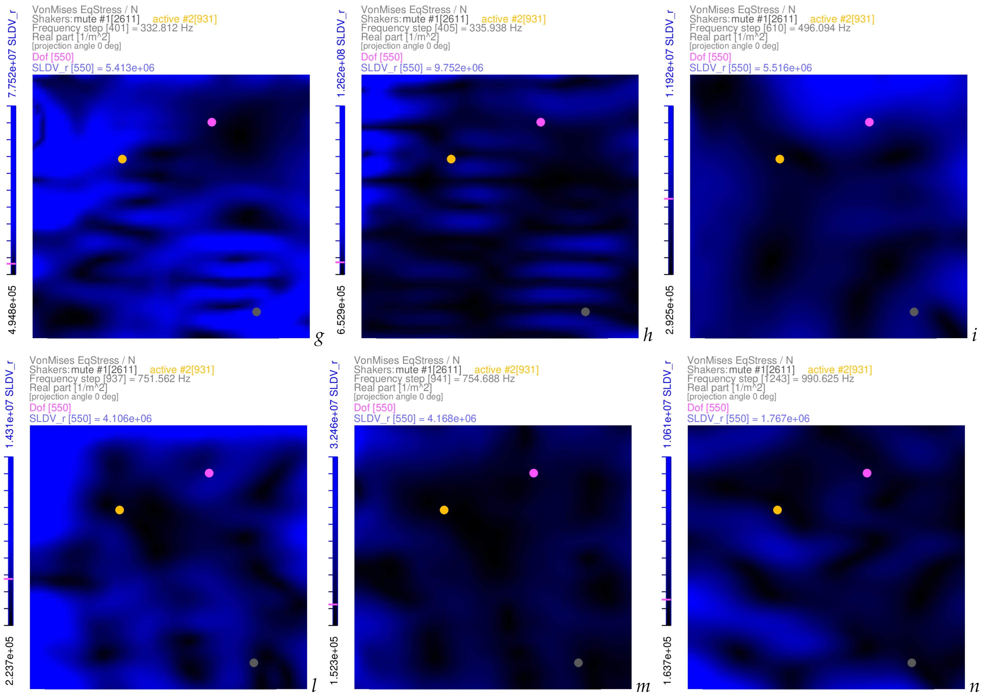
3.1. Examples of Von Mises Equivalent Stress FRFs

Figures 3,4–5,6 were already referenced in Section 2.2.2 to give direct examples of Equation (7), von Mises Equivalent Stress FRF ${\mathit{H}}_{{\mathit{\sigma }}_{\mathit{vM}}}(x,y,\omega )$ evaluations from the two shakers; the quantities are expressed in $[1/m^2]$ and give a precise spatial mapping of the complex amplitude of ${\mathit{H}}_{{\mathit{\sigma }}_{\mathit{vM}}}(x,y,\omega )$, strongly varied in each tile at the specific frequencies highlighted in the captions, due to the underneath ODS, with related measurement errors. In Figures 3,4, the tiles $b,d,f$ markedly show the weaknesses of the mobilities’ estimation from shaker 1, as already underlined in [24,29]. These issues are magnified—in the derivation chain of strains-stresses of Equations (3), (5), (7), despite the advanced numerical tools customised, as in the Appendix of [6]—in the tiles $b,c,d,f,g,h$, but less in l, of Figures 5,6, obtained from shaker 2. The latter was the excitation source with more scanning-related problems in the TEFFMA project, despite the optimal, or very good, point-wise responses from the SLDV instrumentation during the measurement campaign. Despite the scanning-related problems in SLDV-based datasets, it is clear how the complexity of the structural dynamics is well retained from real-life testing, without any simplification, except that of linearity checks. Note how the spatial domain releases clear evidences of compromised measurements, at least in some frequencies: this might be taken into due consideration for refining SHM iterative strategies.

On each tile in Figures 3,4–5,6, with a big magenta dot, the structural dof 550 is highlighted for the frequency domain inquiries of the specific function later proposed. Indeed, dof 550 serves to show the von Mises Equivalent Stress FRF ${H_{{\sigma }_{vM}}}_{550}\left(\omega \right)$ in the whole frequency domain, as in Figure 7a,b from both shakers. In the latter figures, the complex phase clearly denotes a restraint in the range $[-\pi ,-\pi /2]$, due to the specific formulation of Equation (7) and of the functional ${\mathcal{F}}_{vM}\left(\right)$ in Equation (C.2). In the single dof graphs the quality of the shown von Mises Equivalent Stress FRF ${H_{{\sigma }_{vM}}}_{550}\left(\omega \right)$ in the whole frequency domain appears (wrongly) less affected by the scanning-related problems maps at single frequency lines. As written above, therefore, more attention should be paid to the spatial domain for effective diagnosis of the processing chain in successful SHM.

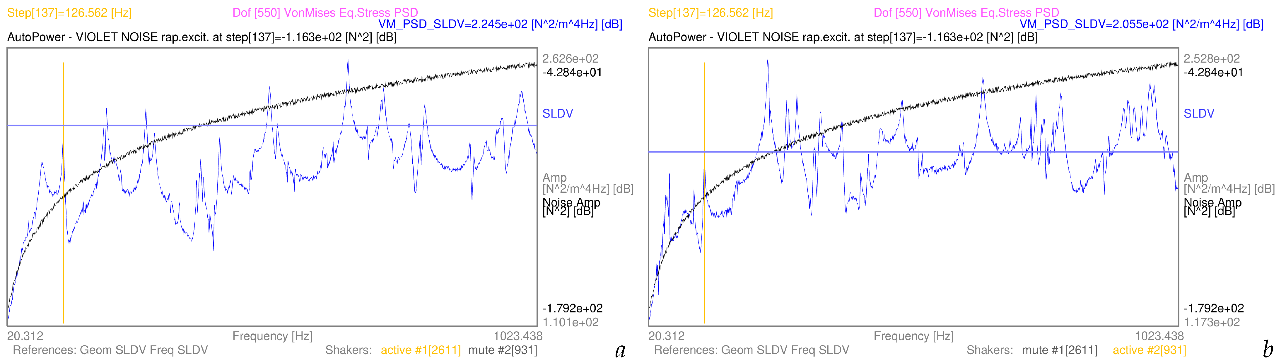
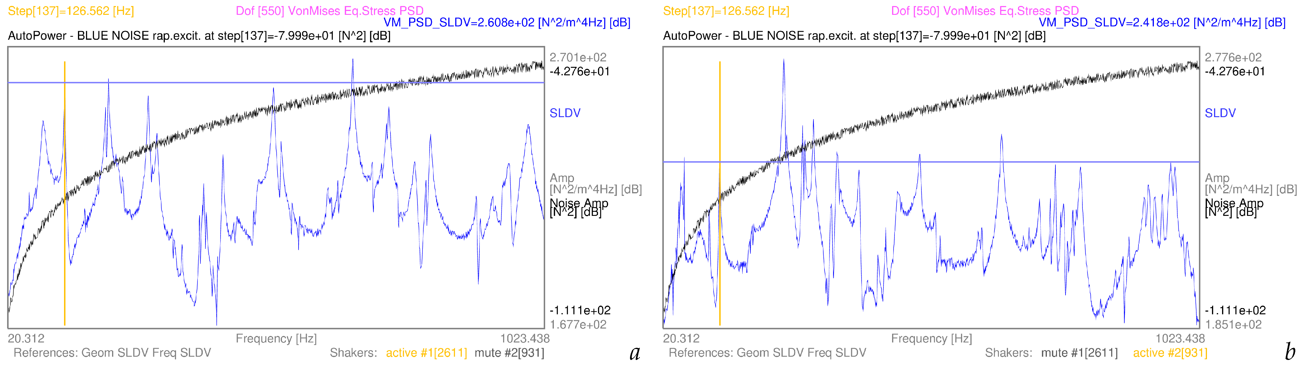
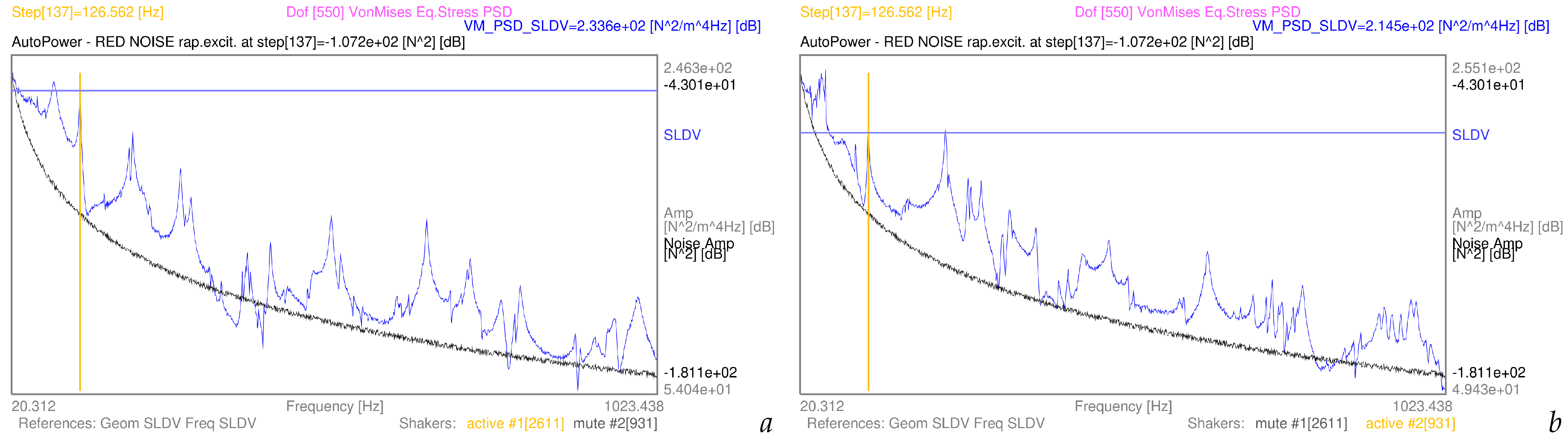
3.2. Examples of Von Mises Equivalent Stress PSDs from Complex-Valued Coloured Noise Excitations

As already commented in [7,8,9,10,11,12,17], changing PSDs maps in Equation (13) are easily obtained starting from the same stress FRFs ${\mathit{H}}_{\mathit{\sigma }}(x,y,\omega )$ in Equation (11), by introducing specific excitation signatures $F\left(\omega \right)$, here shaped in the general complex-valued and randomly-noisy Equation (12) in Section 2.3, and an energy injection point (or shaker), therefore a specific impedance-based experimental model of the structural dynamics. Note that the FRFs of the latter change with the excitation point, because dependent on the nodal lines of the raw receptances. Instead, in EMA [4,5] or in EFFMA [3,16], the modal eigenshapes are independent of the excitations, but are obtained as the modal truncated base that fits—with residues—the FRFs, blended by different participation factors.

Here the $PS{D}_{{\mathrm{\Sigma }}_{vM}}\left(\omega \right)$, extracted from the whole maps, are displayed as log-amplitude graphs by blue curves in Figures 8–11, with also a descriptive title string in blue, while the abscissa and ordinate labels are in grey. In the magenta title the dof of inquiry, the same dof 550 as in the previous figures, is highlighted. In the same Figures 8–11, the Auto-Power-spectrum of the specific excitation is superposed in black curves, labels and text. The modulation of the complex amplitude of the coloured-noise excitation—as the consequence of the specific $\alpha$—has clearly an influence on the output $PS{D}_{{\mathrm{\Sigma }}_{vM}}\left(\omega \right)$. In particular, the shape of the excitation can give emphasis to the different spectral component of the structural dynamic in the experiment-based full-field FRFs. Furthermore, the randomness in the excitation—either in the complex amplitude or in the complex phase, even if not fully visualized due to the nature of PSD- and Auto-Power-spectrum-graphs—is properly transferred to the $PS{D}_{{\mathrm{\Sigma }}_{vM}}\left(\omega \right)$, thanks to the complex-valued formulation of the approach in Equation (12). Note how the excitation signature in the whole spectrum modulates the von Mises Equivalent Stress FRFs in Figure 7. Again, this underlines how real-life excitation spectra can be employed in this approach.

Table 1. Basic statistics of the time-to-failure distributions, according to Equation (14), with the different coloured noises in Equation (12) and excitation location.

Noise Colour	Dof	min	Dof	max	Mean	Std.Dev.	Variance	Skewness	Kurtosis
+ Shaker	min	[h]	max	[h]	[h]	[h]	[h2]	[/]	[/]
violet rap S1	1	2.462e+00	1107	3.240e+04	9.713e+02	2.719e+03	7.394e+06	6.936e+00	5.943e+01
violet rap S2	1	2.510e-01	934	5.300e+03	3.790e+02	5.502e+02	3.027e+05	3.372e+00	1.568e+01
blue rap S1	343	1.661e-01	1687	3.567e+02	3.609e+01	5.053e+01	2.554e+03	2.654e+00	8.724e+00
blue rap S2	1	5.277e-02	2325	1.139e+02	1.554e+01	1.605e+01	2.576e+02	2.173e+00	5.555e+00
white rap S1	1	5.549e-04	699	1.803e-01	3.121e-02	2.384e-02	5.684e-04	2.019e+00	6.452e+00
white rap S2	1	2.773e-04	1452	3.239e-01	3.368e-02	3.753e-02	1.409e-03	3.170e+00	1.364e+01
pink rap S1	1	3.942e+00	756	1.166e+03	1.815e+02	2.068e+02	4.279e+04	2.155e+00	4.525e+00
pink rap S2	1	3.405e-01	1277	2.423e+03	1.062e+02	1.755e+02	3.081e+04	4.862e+00	3.297e+01
red rap S1	2907	1.063e+03	2835	4.354e+05	4.951e+04	5.640e+04	3.180e+09	2.175e+00	6.715e+00
red rap S2	1	1.728e+01	1277	4.926e+05	1.215e+04	3.486e+04	1.215e+09	6.864e+00	5.735e+01

Table 1. Basic statistics of the time-to-failure distributions, according to Equation (14), with the different coloured noises in Equation (12) and excitation location.

Noise Colour	Dof	min	Dof	max	Mean	Std.Dev.	Variance	Skewness	Kurtosis
+ Shaker	min	[h]	max	[h]	[h]	[h]	[h2]	[/]	[/]
violet rap S1	1	2.462e+00	1107	3.240e+04	9.713e+02	2.719e+03	7.394e+06	6.936e+00	5.943e+01
violet rap S2	1	2.510e-01	934	5.300e+03	3.790e+02	5.502e+02	3.027e+05	3.372e+00	1.568e+01
blue rap S1	343	1.661e-01	1687	3.567e+02	3.609e+01	5.053e+01	2.554e+03	2.654e+00	8.724e+00
blue rap S2	1	5.277e-02	2325	1.139e+02	1.554e+01	1.605e+01	2.576e+02	2.173e+00	5.555e+00
white rap S1	1	5.549e-04	699	1.803e-01	3.121e-02	2.384e-02	5.684e-04	2.019e+00	6.452e+00
white rap S2	1	2.773e-04	1452	3.239e-01	3.368e-02	3.753e-02	1.409e-03	3.170e+00	1.364e+01
pink rap S1	1	3.942e+00	756	1.166e+03	1.815e+02	2.068e+02	4.279e+04	2.155e+00	4.525e+00
pink rap S2	1	3.405e-01	1277	2.423e+03	1.062e+02	1.755e+02	3.081e+04	4.862e+00	3.297e+01
red rap S1	2907	1.063e+03	2835	4.354e+05	4.951e+04	5.640e+04	3.180e+09	2.175e+00	6.715e+00
red rap S2	1	1.728e+01	1277	4.926e+05	1.215e+04	3.486e+04	1.215e+09	6.864e+00	5.735e+01

3.3. Examples of Time-to-Failure Distributions with Complex-Valued Coloured Noise Excitations

As stated above in Section 3.2, the choice of the specific coloured noises and the energy injection location brings different von Mises Equivalent Stress PSD maps. But the latter are fed to the cumulative damage and fatigue estimation spectral methods in Section 2.4 and Appendix D to obtain the Equivalent Range of Stress Cycles $S_{eq}(x,y)$ of Equation (D.2). Therefore, a specific evaluation of the Time-to-Failure maps in Equation (14) corresponds to each of the choices. Table 1 gathers the basic statistics of these different choices. Note that also the results from white-rap noise are included, although the Auto Power spectrum of that excitation was not depicted, being the amplitude modulation even among the frequency lines, except for the the randomness in the complex amplitude and phase.

The starting of the crack, or of the failure, is supposed to happen in the dof with the minimal value of each Time-to-Failure distribution, whereas the less injured location is the one with the maximum Time-to-Failure. As highlighted by the basic statistical descriptors (min, max, Mean, Standard Deviation, Variance, Skewness, Kurtosis), each Time-to-Failure distribution is totally deterministic, as the whole approach implies, and has no relation to a Gaussian distribution. Therefore, a strong variability in each Time-to-Failure map is underlined by Table 1, linked to the excitation type and application point. For the specific specimen tested, most of the crack would start in dof 1, at a corner of the sensed region (but slightly inside the plate borders), where the plate undergoes stronger motions in comparison with other positions. Also, looking at the Mean value of the Time-to-Failure maps, it appears that shaker 2 gives generally a shorter expected life than shaker 1, with relatively minor values of Standard Deviation and Variance, except for the white-rap noise excitation. This can be explained by stronger participations of the bending vibrations when excited from shaker 2, again underlining the relevance of the energy injection location in each specific receptances-based formulation. At the same time, it is important to recall the scanning-related problems in SLDV-datasets, especially from shaker 2, which surely have a distorting influence on the weight certain frequencies have in the calculations of $S_{eq}(x,y)$. Again, the quality of the full-field receptances is crucial for a successful SHM.

Figure 12. SLDV-based frequency-to-failure distribution log-amplitude maps of Equation (15), obtained from violet noise-rap excitation, as in Equation (12), from shaker 1: top view in (a) and 3D view in (b).

Figure 12. SLDV-based frequency-to-failure distribution log-amplitude maps of Equation (15), obtained from violet noise-rap excitation, as in Equation (12), from shaker 1: top view in (a) and 3D view in (b).

Figure 13. SLDV-based frequency-to-failure distribution log-amplitude maps of Equation (15), obtained from violet noise-rap excitation, as in Equation (12), from shaker 2: top view in (a) and 3D view in (b).

Figure 13. SLDV-based frequency-to-failure distribution log-amplitude maps of Equation (15), obtained from violet noise-rap excitation, as in Equation (12), from shaker 2: top view in (a) and 3D view in (b).

Figure 14. SLDV-based frequency-to-failure distribution log-amplitude maps of Equation (15), obtained from blue noise-rap excitation, as in Equation (12), from shaker 1: top view in (a) and 3D view in (b).

Figure 14. SLDV-based frequency-to-failure distribution log-amplitude maps of Equation (15), obtained from blue noise-rap excitation, as in Equation (12), from shaker 1: top view in (a) and 3D view in (b).

Figure 15. SLDV-based frequency-to-failure distribution log-amplitude maps of Equation (15), obtained from blue noise-rap excitation, as in Equation (12), from shaker 2: top view in (a) and 3D view in (b).

Figure 15. SLDV-based frequency-to-failure distribution log-amplitude maps of Equation (15), obtained from blue noise-rap excitation, as in Equation (12), from shaker 2: top view in (a) and 3D view in (b).

Figure 16. SLDV-based frequency-to-failure distribution log-amplitude maps of Equation (15), obtained from pink noise-rap excitation, as in Equation (12), from shaker 1: top view in (a) and 3D view in (b).

Figure 16. SLDV-based frequency-to-failure distribution log-amplitude maps of Equation (15), obtained from pink noise-rap excitation, as in Equation (12), from shaker 1: top view in (a) and 3D view in (b).

Figure 17. SLDV-based frequency-to-failure distribution log-amplitude maps of Equation (15), obtained from pink noise-rap excitation, as in Equation (12), from shaker 2: top view in (a) and 3D view in (b).

Figure 17. SLDV-based frequency-to-failure distribution log-amplitude maps of Equation (15), obtained from pink noise-rap excitation, as in Equation (12), from shaker 2: top view in (a) and 3D view in (b).

Figure 18. SLDV-based frequency-to-failure distribution log-amplitude maps of Equation (15), obtained from red noise-rap excitation, as in Equation (12), from shaker 1: top view in (a) and 3D view in (b).

Figure 18. SLDV-based frequency-to-failure distribution log-amplitude maps of Equation (15), obtained from red noise-rap excitation, as in Equation (12), from shaker 1: top view in (a) and 3D view in (b).

Figure 19. SLDV-based frequency-to-failure distribution log-amplitude maps of Equation (15), obtained from red noise-rap excitation, as in Equation (12), from shaker 2: top view in (a) and 3D view in (b).

Figure 19. SLDV-based frequency-to-failure distribution log-amplitude maps of Equation (15), obtained from red noise-rap excitation, as in Equation (12), from shaker 2: top view in (a) and 3D view in (b).

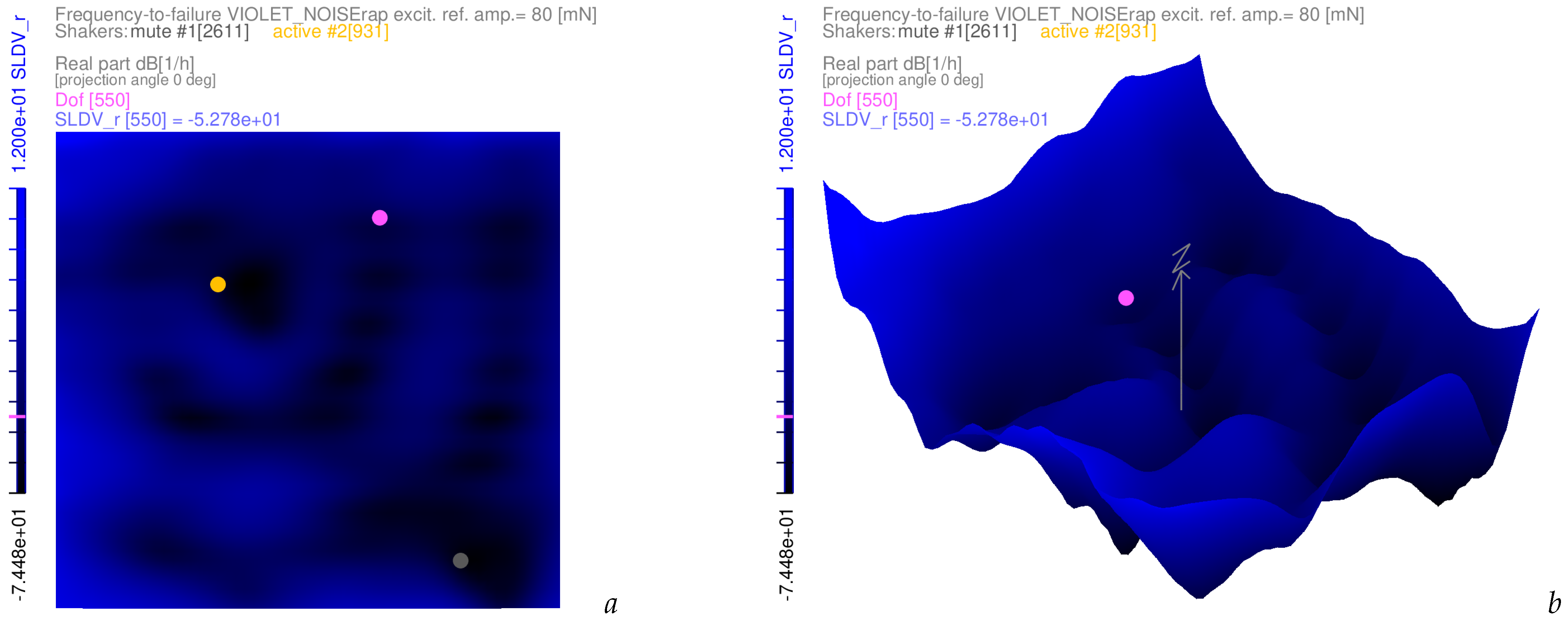
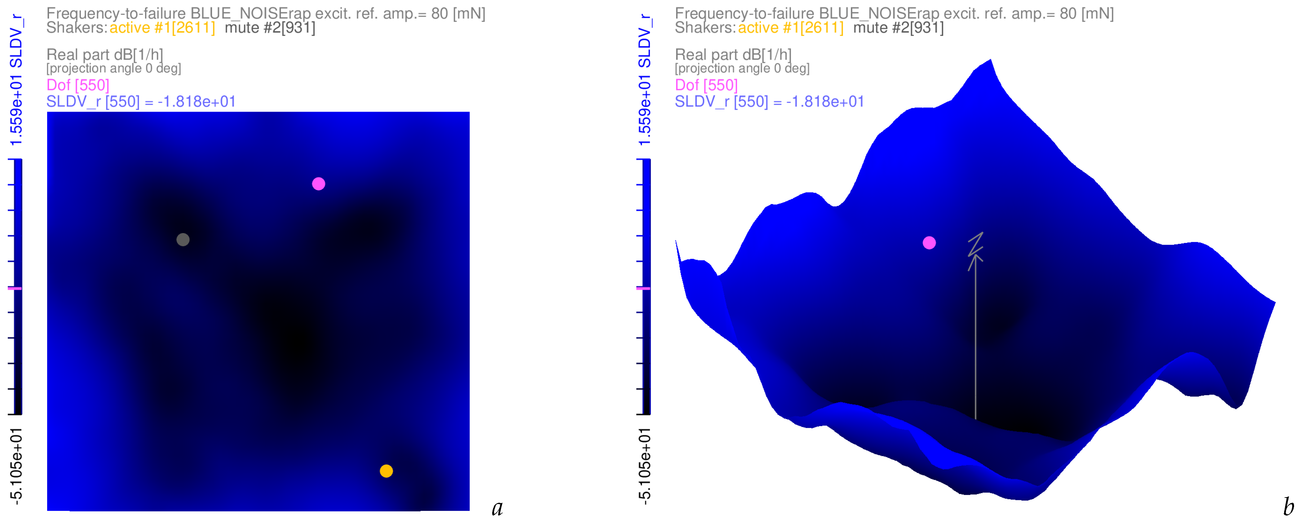
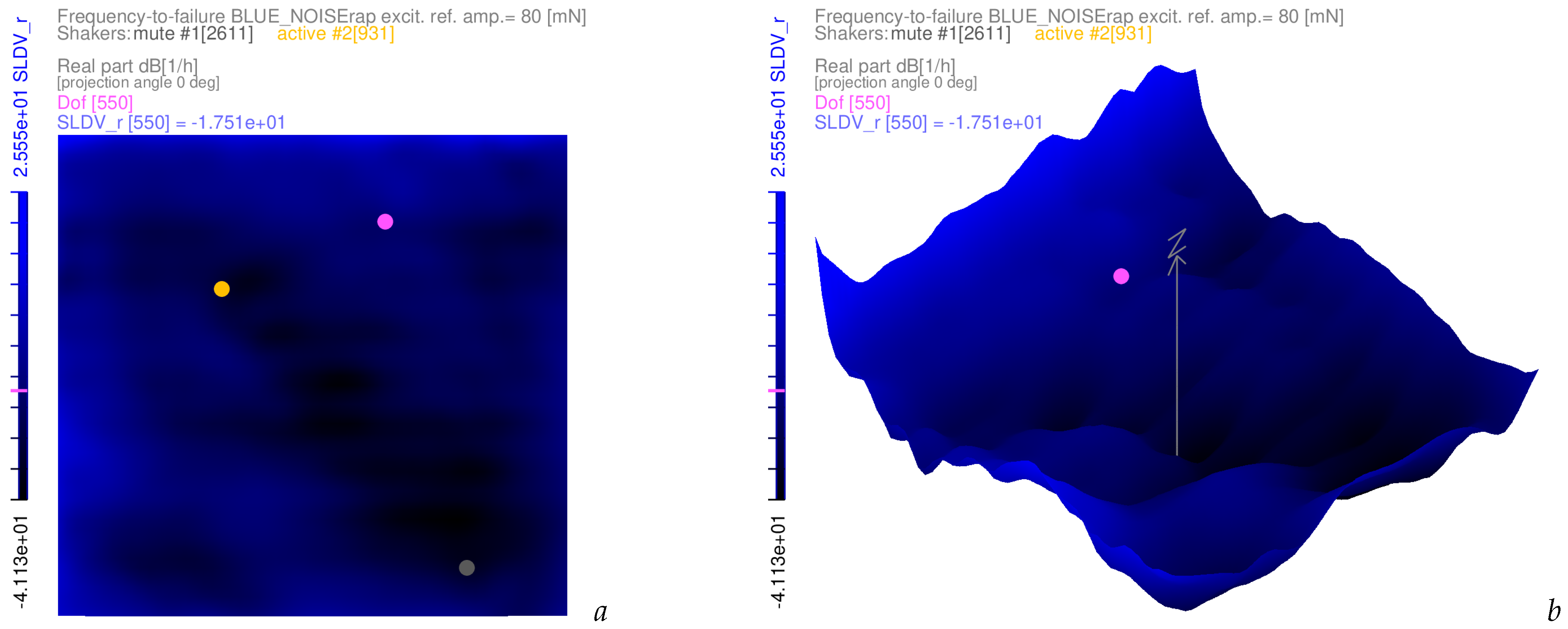
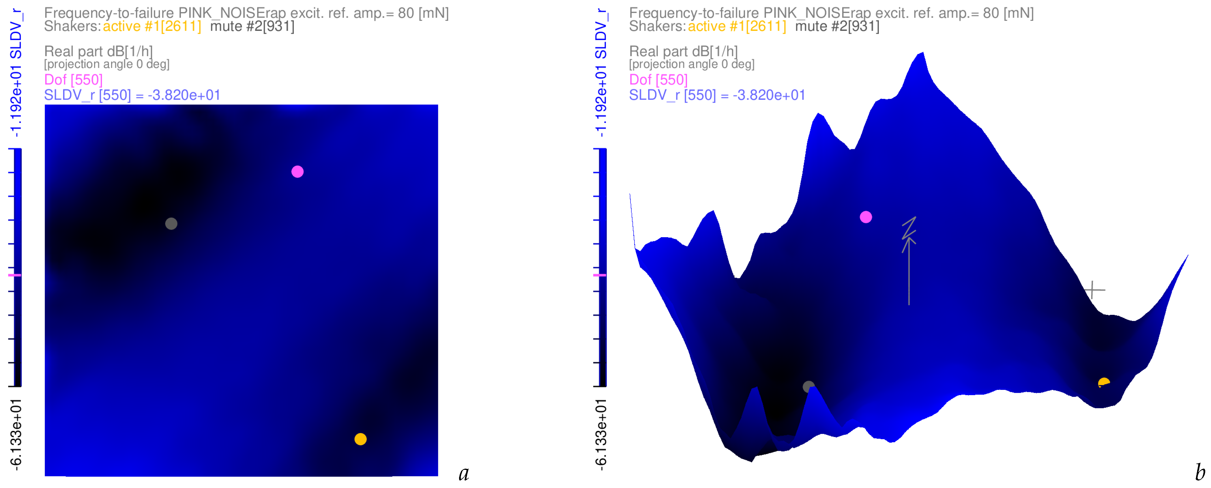
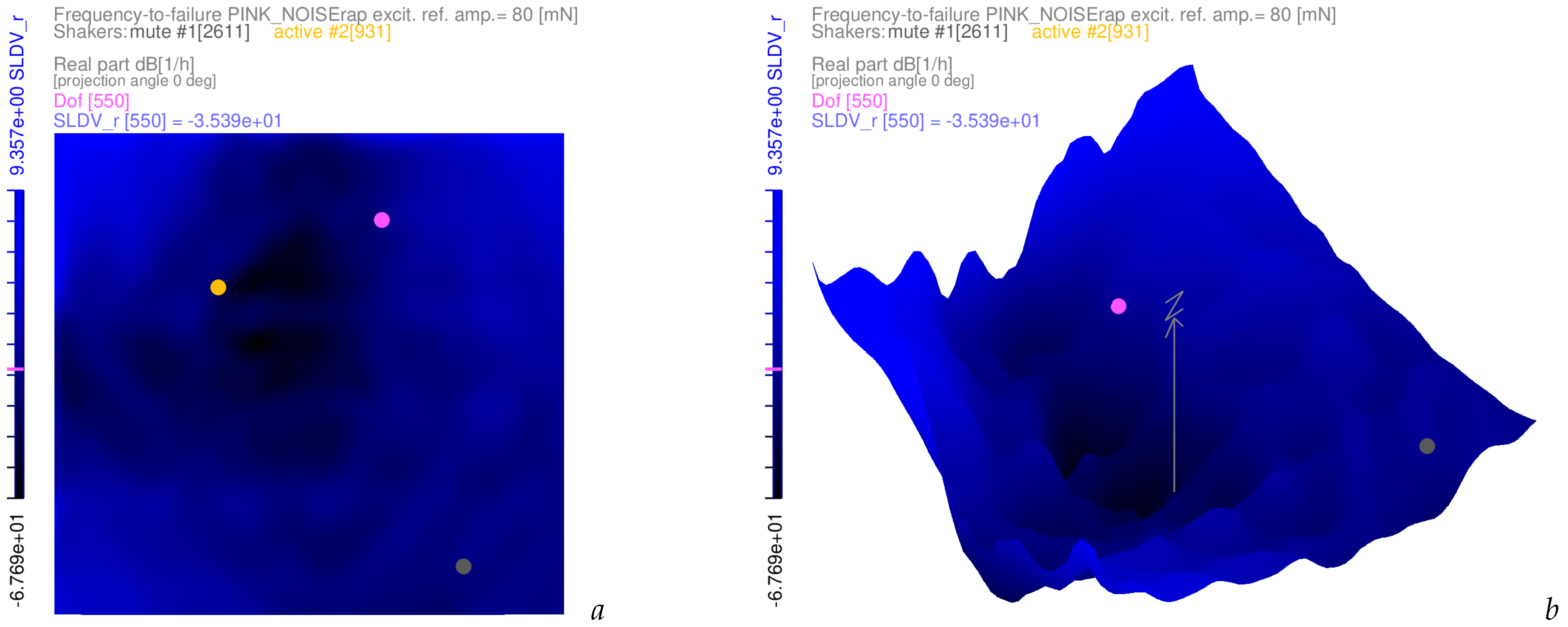
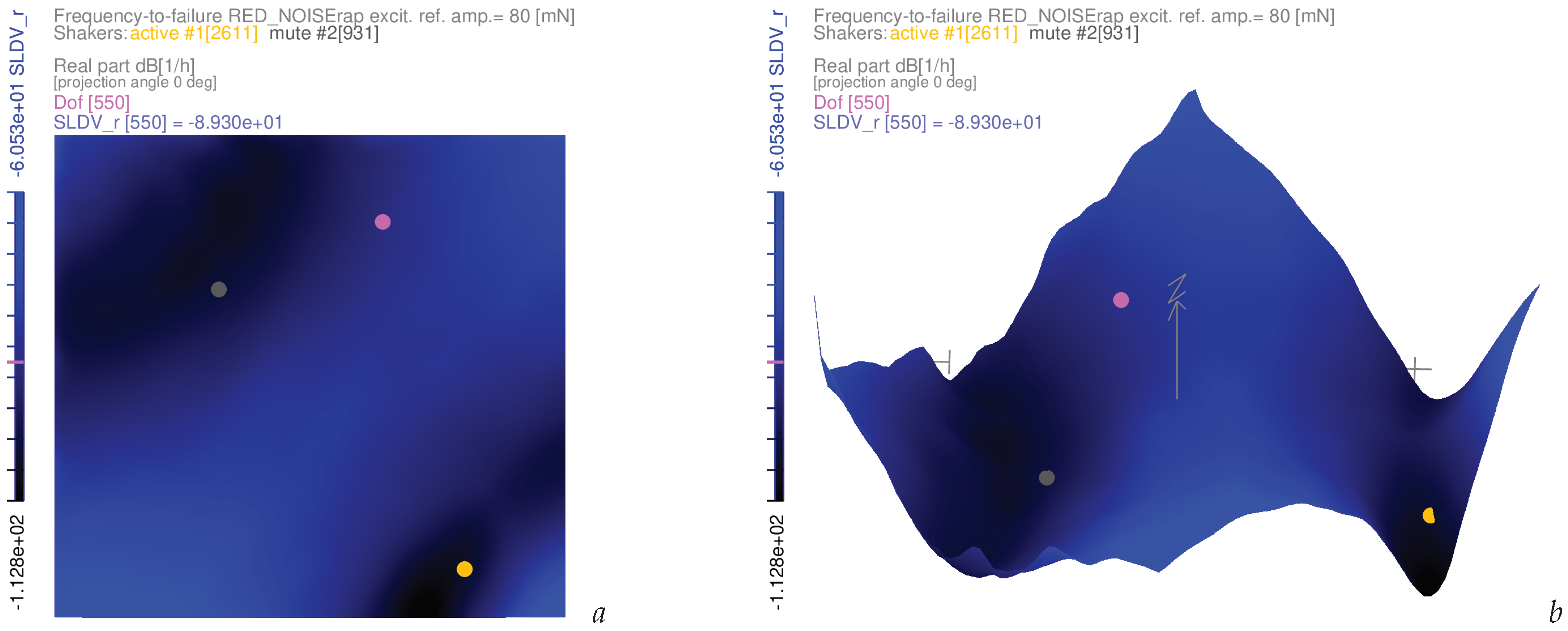
3.4. Examples of Frequency-to-Failure Maps with Complex-Valued Coloured Noise Excitations

Similar evaluations as those made in Section 3.3 can be here run, with a focus on the Frequency-to-Failure maps, coming from Equation (15). The latter are again obtained by means of the Equivalent Range of Stress Cycles $S_{eq}(x,y)$ of Equation (D.2), with the specific choice of the coloured noise, the energy injection location and related von Mises Equivalent Stress PSD map. Therefore, to each of the choices corresponds a specific evaluation of the Frequency-to-Failure map in Equation (15). In these evaluations, the starting of the failure should happen in the dof with the maximal value of each Frequency-to-Failure distribution, whereas the less injured point is the one with the minimal Frequency-to-Failure value. Being Equation (15) the reciprocal of Equation (14), a strong variability is also expected in each Frequency-to-Failure map, as can be seen in Figures 12–19, where the results are shown along the log-Z axis (in dB[1/h]), together with brighter blue tones on higher values, to better highlight where the failure should start first. Similar considerations can be made about the stronger solicitation in the corners of the sensed region (under which the restraining cables are attached) and about the structured noise (see [29]), with related influences. However, as for the Time-to-Failure distributions in Section 3.3, a marked variability can be found inside the spatial domain, due to the fusion of excitation signature and fully populated experiment-based full-field receptances.

The violet noise-rap excitation signal (Equation (12), $\alpha =-2$, with randomness in the complex amplitude and phase as all the rap signals) is responsible, through the ${PSD}_{{\mathrm{\Sigma }}_{vM}}(x,y,\omega )$ in Equation (13) for the graphs in Figure 8, of the $F_{failure}(x,y)$ maps of Figures 12–13. Instead, the blue noise-rap signal (Equation (12), $\alpha =-1$), thanks to the ${PSD}_{{\mathrm{\Sigma }}_{vM}}(x,y,\omega )$ shown in Figure 9, generates the $F_{failure}(x,y)$ distributions of Figures 14–15. Instead, by reversing the sign of $\alpha$, the pink noise-rap excitation (Equation (12), $\alpha =1$) is simulated; this is the source to obtain the ${PSD}_{{\mathrm{\Sigma }}_{vM}}(x,y,\omega )$ for the graphs in Figure 10 and for $F_{failure}(x,y)$ maps of Figures 16–17. The last simulations here shown come from the selection of the red noise-rap excitation (Equation (12), $\alpha =2$); the red noise-rap excitation multiplies the previous ${\mathit{H}}_{\mathit{\sigma }}(x,y,\omega )$, to obtain the $PS{D}_{{\mathrm{\Sigma }}_{vM}}(x,y,\omega )$ shown in Figure 11 and used in Equation (15) to evaluate the $F_{failure}(x,y)$ distributions in Figures 18–19.

As in Section 3.3, the change of the structure’s task—the couple of the spectrum of the excitation $F\left(\omega \right)$ and its energy injection location—brings very different $F_{failure}(x,y)$ maps and expected life scenarios, where the accurate assessment of the dynamic behaviour of the real component, or part, is of uttermost importance for the reliability of any SHM, as in this experiment-based approach no assumptions nor approximations were made to come to any artificial/purely numerical structural model.

4. Discussion

It is important to revisit what proposed in Sections 2–3 from the point of view of the SHM, because the whole methodology has made no assumptions about the structure to simulate the expected life distribution under a specific task. Indeed, this approach is permeated by the experimental assessment of the structural dynamics and of the dynamic loading. But, as demonstrated by the examples of Section 3, the strong variability in the results can be explained only by possessing the whole reliable knowledge of the task-oriented dynamic event. Optical full-field measurement techniques, thanks to their qualities mentioned in Section 1, can extend the sensing to a fully-populated spatial domain, without the need of an a-priori selection of locations for the transducers. Furthermore, the shown results—of a single dof (here 550) in the whole map—demonstrate that, without imposing any simplifying assumption that might deteriorate the understanding of the dynamic responses, the selection of lumped sensors becomes quite complex in changing scenarios, if not impracticable. However, the quality of the structural measurements has an impact on the whole simulation chain, as underlined especially in Section 3.1, where at some frequency lines the noisy SLDV mobilities gave misinterpretations of the derived quantities due to scanning-related issues during the measurement campaign [18,24,29]. Note that the image-based full-field receptances proved in [6,7,8,9,10,11,12] to release much spatially smoother datasets than scanning-based techniques, without further noise reduction processing.

As anticipated in Section 1, SHM should extend its assessments of the structural dynamics and loadings during the whole life of the components, especially when ageing, unpredicted accidents or changes happen. These assessments should be run periodically, to change iteratively the expectations on the duration of the parts and on the starting failure location, and to adapt the maintenance programs for them. This is the hard lesson learned from these simulated results: changes to the dynamic behaviour of the structure, as well as on the loadings, result in marked variability of the expected life distribution, therefore of the many managing and processing activities that can follow for a fruitful SHM.

Also manufacturing can get advantages from this approach, specifically for allocating material where needed in mass optimisations and for determining technological aspects for the most solicited areas. Furthermore, quality assessments to find defects during the production of parts can be based on the same achievements, as in [8,12].

Future research activities are needed to assess the validity of the whole approach, e.g. by reaching the failure start and obtain the cumulative damage distribution in simple specimens, like the plate here used, under known excitation and environmental conditions. Once the procedure proves its accuracy on simple test cases, the experiment-based full-field fatigue hybrid predictions and SHM can be extended to more complex parts or assemblies.

5. Conclusions

In this paper SLDV mobilities were the experiment-based datasets’ sources—instead of other spatially-cleaner image-based full-field techniques—for retaining the real dynamic behaviour of the lightweight structure, a simple thin plate, and for giving clear examples from a measurement instrumentation, which is quite widespread among the non-contacting technologies. Also with SLDV mobilities the following achievements were possible, with no further modelling assumption nor lumped sensors’ selection:

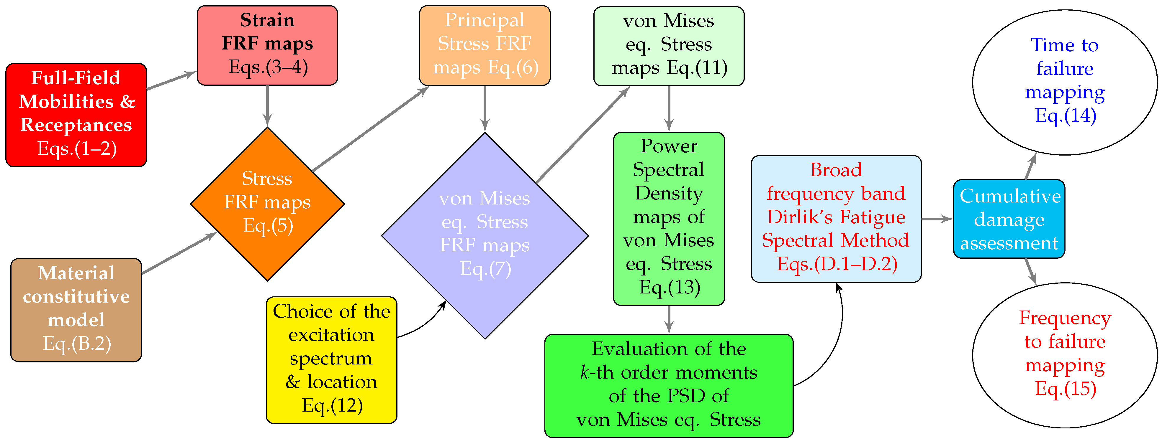
• estimation of Strain-FRF maps;
• evaluation of Stress-FRF maps by a proper constitutive model of the material;
• evaluation of von Mises Equivalent Stress-FRF maps;
• evaluation of von Mises Equivalent Stress-PSDs, as dependent on the selected complex-valued spectrum and location of the excitation;
• evaluation of high spatial resolution maps of cumulative damage and life expectations by means of fatigue spectral methods and excitation location and spectra.

This paper has shown how an experiment-based updated and reliable knowledge—of the task-oriented responses in a dynamically loaded structure—can improve a proper SHM, especially in changing and ageing scenarios. A complete approach was deployed to exploit the full-field receptances of the structure, to describe the actual realisation of the components under analysis without numerical synthetic models, and to use all the components of the complex-valued spectrum of the excitations, to be able to properly treat experimental evidences and recordings, all done without specific assumptions, except for linearity.

The paper has shown the strong dependency of the fatigue life distribution on the task the component has to fulfil, together with the relevance of the accuracy of the SLDV mobilities in assuring reliable estimation of the actual structural dynamics in the whole approach. Iterative sensing of the component and updated knowledge of the loading become milestones for advanced SHM, in order to better manage maintenance and operations of changing, or ageing, task-oriented structural parts.

References

1. Friswell, M.; Mottershead, J.E. Finite Element Model Updating in Structural Dynamics; Solid Mechanics and Its Applications; Kuwler Academic Publishers & Springer Science+Business Media: Dordrecht, The Netherlands, 1995; p. 292. ISBN 978-0-7923-3431-6. [Google Scholar]
2. Mottershead, J.E.; Link, M.; Friswell, M.I. The sensitivity method in finite element model updating: A tutorial. Mech. Syst. Signal Process. 2011, 25, 2275–2296. [Google Scholar] [CrossRef]
3. Zanarini, A. Full field optical measurements in experimental modal analysis and model updating. J. Sound Vib. 2019, 442, 817–842. [Google Scholar] [CrossRef]
4. Ewins, D.J. Modal Testing – Theory, Practice and Application, 2nd ed.; Research Studies Press Ltd.: Baldock, Hertfordshire, UK, 2000; p. 400. ISBN 978-0-86380-218-8. [Google Scholar]
5. Heylen, W.; Lammens, S.; Sas, P. Modal Analysis Theory and Testing, 2nd ed.; Katholieke Universiteit Leuven: Leuven, Belgium, 1998; ISBN 90-73802-61-X. [Google Scholar]
6. Zanarini, A. Chasing the high-resolution mapping of rotational and strain FRFs as receptance processing from different full-field optical measuring technologies. Mech. Syst. Signal Process. 2022, 166, 108428. [Google Scholar] [CrossRef]
7. Zanarini, A. On the defect tolerance by fatigue spectral methods based on full-field dynamic testing. Procedia Struct. Integr. 2022, 37, 525–532, Proceedings of The 4th International Conference on Structural Integrity, 30 August–1 September 2021. [Google Scholar] [CrossRef]
8. Zanarini, A. Introducing the concept of defect tolerance by fatigue spectral methods based on full-field frequency response function testing and dynamic excitation signature. Int. J. Fatigue 2022, 165, 107184. [Google Scholar] [CrossRef]
9. Zanarini, A. About the excitation dependency of risk tolerance mapping in dynamically loaded structures. In Proceedings of the ISMA2022 Including USD2022—International Conference on Noise and Vibration Engineering, Leuven, Belgium, 12–14 September 2022; pp. 3804–3818, in Vol. Structural Health Monitoring. Available online: https://past.isma-isaac.be/downloads/isma2022/proceedings/Contribution_208_proceeding_3.pdf (accessed on 22 March 2025).
10. Zanarini, A. Risk Tolerance Mapping in Dynamically Loaded Structures as Excitation Dependency by Means of Full-Field Receptances. In Proceedings of the IMAC XLI—International Modal Analysis Conference—Keeping IMAC Weird: Traditional and Non-Traditional Applications of Structural Dynamics, Austin, TX, USA, 13–16 February 2023; Computer Vision & Laser Vibrometry, Volume 6, Conference Proceedings of the Society for Experimental Mechanics Series. Baqersad, J., Di Maio, D., Eds.; Springer Nature: Cham, Switzerland; SEM Society for Experimental Mechanics: Bethel, CT, USA, 2023; Chapter 9; pp. 43–56. [Google Scholar] [CrossRef]
11. Zanarini, A. Exploiting DIC-based full-field receptances in mapping the defect acceptance for dynamically loaded components. Procedia Struct. Integr. 2024, 54C, 99–106, Proceedings of The 5th International Conference on Structural Integrity, 28 August–1 September, 2023. [Google Scholar] [CrossRef]
12. Zanarini, A. Mapping the defect acceptance for dynamically loaded components by exploiting DIC-based full-field receptances. Eng. Fail. Anal. 2024, 163, 108385. [Google Scholar] [CrossRef]
13. Van der Auweraer, H.; Dierckx, B.; Haberstok, C.; Freymann, R.; Vanlanduit, S. Structural modelling of car panels using holographic modal analysis. In Proceedings of the 1999 Noise and Vibration Conference, Traverse City, MI, USA, 17–20 May 1999; Volume 3, pp. 1495–1506, SAE P-342. [Google Scholar] [CrossRef]
14. Van der Auweraer, H.; Steinbichler, H.; Haberstok, C.; Freymann, R.; Storer, D. Integration of pulsed-laser ESPI with spatial domain modal analysis: Results from the SALOME project. In Proceedings of the 4th International Conference on Vibration Measurements by Laser Techniques: Advances and Applications, Ancona, Italy, 20–23 June 2000; SPIE: Bellingham, WA, USA, 2000; Volume 4072, pp. 313–322. [Google Scholar] [CrossRef]
15. Van der Auweraer, H.; Steinbichler, H.; Haberstok, C.; Freymann, R.; Storer, D.; Linet, V. Industrial Applications of Pulsed-laser ESPI vibration analysis. In Proceedings of the XIX IMAC, Kissimmee, FL, USA, 5–8 February 2001; Society for Experimental Mechanics (SEM): Bethel, CT, USA, 2001; pp. 490–496. [Google Scholar]
16. Van der Auweraer, H.; Steinbichler, H.; Vanlanduit, S.; Haberstok, C.; Freymann, R.; Storer, D.; Linet, V. Application of stroboscopic and pulsed-laser electronic speckle pattern interferometry (ESPI) to modal analysis problems. Meas. Sci. Technol. 2002, 13, 451–463. [Google Scholar] [CrossRef]
17. Zanarini, A. Broad frequency band full field measurements for advanced applications: Point-wise comparisons between optical technologies. Mech. Syst. Signal Process. 2018, 98, 968–999. [Google Scholar] [CrossRef]
18. Zanarini, A. Competing optical instruments for the estimation of Full Field FRFs. Measurement 2019, 140, 100–119. [Google Scholar] [CrossRef]
19. Baqersad, J.; Poozesh, P.; Niezrecki, C.; Avitabile, P. Photogrammetry and optical methods in structural dynamics—A review. Mech. Syst. Signal Process. 2017, 86, 17–34, in SI: Full-field, non-contact vibration measurement methods: comparisons and applications. [Google Scholar] [CrossRef]
20. Wang, W.; Mottershead, J.E.; Ihle, A.; Siebert, T.; Schubach, H.R. Finite element model updating from full-field vibration measurement using digital image correlation. J. Sound Vib. 2011, 330, 1599–1620. [Google Scholar] [CrossRef]
21. Wang, W.; Mottershead, J.; Siebert, T.; Pipino, A. Frequency response functions of shape features from full-field vibration measurements using digital image correlation. Mech. Syst. Signal Process. 2011, 28, 333–347. [Google Scholar] [CrossRef]
22. LeBlanc, B.; Niezrecki, C.; Avitabile, P.; Sherwood, J.; Chen, J. Surface Stitching of a Wind Turbine Blade Using Digital Image Correlation. In Topics in Modal Analysis II, Proceedings of the 30th IMAC, A Conference on Structural Dynamics, SEM; Allemang, R., De Clerck, J., Niezrecki, C., Blough, J., Eds.; Springer: New York, NY, USA, 2012; Volume 6, pp. 277–284. [Google Scholar] [CrossRef]
23. Ehrhardt, D.A.; Allen, M.S.; Yang, S.; Beberniss, T.J. Full-field linear and nonlinear measurements using Continuous-Scan Laser Doppler Vibrometry and high speed three-dimensional Digital Image Correlation. Mech. Syst. Signal Process. 2017, 86, 82–97. [Google Scholar] [CrossRef]
24. Zanarini, A. On the making of precise comparisons with optical full field technologies in NVH. In Proceedings of the ISMA2020 Including USD2020—International Conference on Noise and Vibration Engineering, Leuven, Belgium, 7–9 September 2020; pp. 2293–2308, in Vol. Optical methods and computer vision for vibration engineering. Available online: https://past.isma-isaac.be/downloads/isma2020/proceedings/Contribution_695_proceeding_3.pdf (accessed on 22 March 2025).
25. Liu, W.; Ewins, D. The Importance Assessment of RDOF in FRF Coupling Analysis. In Proceedings of the IMAC 17th Conference, Kissimmee, FL, USA, 8–11 February 1999; Society for Experimental Mechanics (SEM): Bethel, CT, USA, 1999; pp. 1481–1487. Available online: https://citeseerx.ist.psu.edu/document?repid=rep1&type=pdf&doi=c44ebc7b37f462e47b44aee1acb1f9de704e92d6 (accessed on 22 March 2025).
26. Research Network. QUATTRO Brite-Euram Project No: BE 97-4184; Technical Report; European Commision Research Framework Programs: Brussels, Belgium, 1998. [Google Scholar]
27. Haeussler, M.; Klaassen, S.; Rixen, D. Experimental twelve degree of freedom rubber isolator models for use in substructuring assemblies. J. Sound Vib. 2020, 474, 115253. [Google Scholar] [CrossRef]
28. Zanarini, A. On the exploitation of multiple 3D full-field pulsed ESPI measurements in damage location assessment. Procedia Struct. Integr. 2022, 37, 517–524, Proceedings of The 4th International Conference on Structural Integrity, 30 August–1 September 2021. [Google Scholar] [CrossRef]
29. Zanarini, A. On the influence of scattered errors over full-field receptances in the Rayleigh integral approximation of sound radiation from a vibrating plate. Acoustics 2023, 5, 948–986. [Google Scholar] [CrossRef]
30. Zanarini, A. Assessing the retrieval procedure of complex-valued forces from airborne pressure fields by means of DIC-based full-field receptances in simplified pseudo-inverse vibro-acoustics. Aerosp. Sci. Technol. 2024, 157, 109757. [Google Scholar] [CrossRef]
31. Forsyth, P. Fatigue damage and crack growth in aluminium alloys. Acta Metall. 1963, 11, 703–715, in SI: Mechanisms of fatigue in crystalline solids. [Google Scholar] [CrossRef]
32. Mao, H.; Mahadevan, S. Fatigue damage modelling of composite materials. Compos. Struct. 2002, 58, 405–410. [Google Scholar] [CrossRef]
33. Kyanka, G.H. Fatigue properties of wood and wood composites. Int. J. Fract. 1980, 16, 609–616. [Google Scholar] [CrossRef]
34. Smith, I.; Landis, E.; Gong, M. Fracture and Fatigue in Wood; Wiley: Hoboken, NJ, USA, 2003; p. 248. ISBN 978-0-471-48708-1. [Google Scholar]
35. Leyens, C.; Peters, M. (Eds.) Titanium and Titanium Alloys: Fundamentals and Applications; Wiley-VCH Verlag GmbH & Co. KGaA: Weinheim, Germany, 2003; ISBN 9783527305346. [Google Scholar] [CrossRef]
36. Farahani, B.V.; Direito, F.; Sousa, P.J.; Tavares, P.J.; Infante, V.; Moreira, P.P. Crack tip monitoring by multiscale optical experimental techniques. Int. J. Fatigue 2022, 155, 106610. [Google Scholar] [CrossRef]
37. Lesiuk, G.; Nykyforchyn, H.; Zvirko, O.; Mech, R.; Babiarczuk, B.; Duda, S.; Maria De Arrabida Farelo, J.; Correia, J.A. Analysis of the Deceleration Methods of Fatigue Crack Growth Rates under Mode I Loading Type in Pearlitic Rail Steel. Metals 2021, 11, 584. [Google Scholar] [CrossRef]
38. Krechkovska, H.; Student, O.; Lesiuk, G.; Correia, J. Features of the microstructural and mechanical degradation of long term operated mild steel. Int. J. Struct. Integr. 2018, 9, 296–306. [Google Scholar] [CrossRef]
39. Lesiuk, G.; Correia, J.A.; Krechkovska, H.V.; Pekalski, G.; Jesus, A.M.d.; Student, O. Degradation Theory of Long Term Operated Materials and Structures; Springer International Publishing: Cham, Switzerland, 2021; pp. 1–215. [Google Scholar] [CrossRef]
40. Ahmad, Z. (Ed.) Principles of Corrosion Engineering and Corrosion Control; Elsevier & Butterworth-Heinemann: Oxford, UK, 2006; pp. 1–656. [Google Scholar] [CrossRef]
41. Gao, J.W.; Dai, G.Z.; Li, Q.Z.; Zhang, M.N.; Zhu, S.P.; Correia, J.A.; Lesiuk, G.; De Jesus, A.M. Fatigue assessment of EA4T railway axles under artificial surface damage. Int. J. Fatigue 2021, 146, 106157. [Google Scholar] [CrossRef]
42. Gao, J.W.; Yu, M.H.; Liao, D.; Zhu, S.P.; Han, J.; Lesiuk, G.; Correia, J.A.; De Jesus, A.M. Fatigue and damage tolerance assessment of induction hardened S38C axles under different foreign objects. Int. J. Fatigue 2021, 149, 106276. [Google Scholar] [CrossRef]
43. Buch, A. Prediction of the comparative fatigue performance for realistic loading distributions. Prog. Aerosp. Sci. 1997, 33, 391–430. [Google Scholar] [CrossRef]
44. Fatemi, A.; Yang, L. Cumulative fatigue damage and life prediction theories: A survey of the state of the art for homogeneous materials. Int. J. Fatigue 1998, 20, 9–34. [Google Scholar] [CrossRef]
45. George, T.J.; Seidt, J.; Shen, M.H.H.; Nicholas, T.; Cross, C.J. Development of a novel vibration-based fatigue testing methodology. Int. J. Fatigue 2004, 26, 474–486. [Google Scholar] [CrossRef]
46. Dirlik, T. Application of Computers in Fatigue Analysis. Ph.D. Thesis, University of Warwick, Coventry, UK, 1985. Available online: https://wrap.warwick.ac.uk/id/eprint/2949/ (accessed on 22 March 2025).
47. ESDU. Spectral methods for the estimation of fatigue life 06011. In Estimation of Fatigue Life of Structures Subjected to Random Loading; Vibration and Acoustic Fatigue Series; ESDU International Plc: London, UK, 2006; Volume 9, pp. 1–56. [Google Scholar]
48. Dowling, E.N. Estimating Fatigue Life. In Fatigue and Fracture; ASM Handbook; ASM International Handbook Committee: Novelty, OH, USA, 1996; Volume 19, pp. 250–262. [Google Scholar]
49. Benasciutti, D.; Tovo, R. Spectral methods for lifetime prediction under wide-band stationary random processes. Int. J. Fatigue 2005, 27, 867–877, in SI: Cumulative Fatigue Damage Conference – University of Seville 2003.. [Google Scholar] [CrossRef]
50. Dirlik, T.; Benasciutti, D. Dirlik and Tovo-Benasciutti Spectral Methods in Vibration Fatigue: A Review with a Historical Perspective. Metals 2021, 11, 1333. [Google Scholar] [CrossRef]
51. Shang, D.G.; Wang, D.K.; Li, M.; Yao, W.X. Local stress-strain field intensity approach to fatigue life prediction under random cyclic loading. Int. J. Fatigue 2001, 23, 903–910. [Google Scholar] [CrossRef]
52. Lynn, A.K.; DuQuesnay, D.L. Computer simulation of variable amplitude fatigue crack initiation behaviour using a new strain-based cumulative damage model. Int. J. Fatigue 2003, 24, 977–986. [Google Scholar] [CrossRef]
53. Koh, S.K. Fatigue damage evaluation of a high pressure tube steel using cycle strain energy density. Int. J. Press. Vessel. Pip. 2002, 79, 791–798. [Google Scholar] [CrossRef]
54. Lagoda, T. Energy models for fatigue life estimation under uniaxial random loading. Part I: The model elaboration. Int. J. Fatigue 2001, 23, 467–480. [Google Scholar] [CrossRef]
55. Lagoda, T. Energy models for fatigue life estimation under uniaxial random loading. Part II: Verification of the model. Int. J. Fatigue 2001, 23, 481–489. [Google Scholar] [CrossRef]
56. Ling, J.; Pan, J. An engineering method for reliability analyses of mechanical structures for long fatigue lives. Reliab. Eng. Syst. Saf. 1997, 56, 135–142. [Google Scholar] [CrossRef]
57. Kuroda, M. Extremely low cycle fatigue life prediction based on a new cumulative fatigue damage model. Int. J. Fatigue 2001, 24, 699–703. [Google Scholar] [CrossRef]
58. ESDU. Fatigue damage and life under random loading 06009. In Estimation of Fatigue Life of Structures Subjected to Random Loading; Vibration and Acoustic Fatigue Series; ESDU International Plc: London, UK, 2006; Volume 9, pp. 1–41. [Google Scholar]
59. Marines, I.; Bin, X.; Bathias, C. An understanding of very high cycle fatigue of metals. Int. J. Fatigue 2003, 25, 1101–1107. [Google Scholar] [CrossRef]
60. Sherratt, F.; Bishop, N.; Dirlik, T. Predicting fatigue life from frequency domain data. J. Eng. Integr. Soc. (EIS) 2005, 18, 12–16. Available online: https://www.researchgate.net/publication/284415325_Predicting_fatigue_life_from_frequency_domain_data (accessed on 22 March 2025).
61. Lee, Y.L.; Tjhung, T.; Jordan, A. A life prediction model for welded joints under multiaxial variable amplitude loading histories. Int. J. Fatigue 2007, 29, 1162–1173. [Google Scholar] [CrossRef]
62. Wolfsteiner, P.; Sedlmair, S. Deriving Gaussian Fatigue Test Spectra from Measured non Gaussian Service Spectra. Procedia Eng. 2015, 101, 543–551, in SI: 3rd International Conference on Material and Component Performance under Variable Amplitude Loading, VAL 2015, Eds. J. Papuga and M. Ruzicka. [Google Scholar] [CrossRef]
63. Sui, G.; Zhang, Y. Response spectrum method for fatigue damage assessment of mechanical systems. Int. J. Fatigue 2023, 166, 107278. [Google Scholar] [CrossRef]
64. McDowell, D.L. Multiaxial Fatigue Strength. In Fatigue and Fracture; ASM Handbook; ASM International Handbook Committee: Novelty, OH, USA, 1996; Volume 19, pp. 263–273. [Google Scholar]
65. Cameron, D.W. Fatigue Properties in Engineering. In Fatigue and Fracture; ASM Handbook; ASM International Handbook Committee: Novelty, OH, USA, 1996; Volume 19, pp. 15–26. [Google Scholar]
66. ASM. Parameters for Estimating Fatigue Life. In Fatigue and Fracture; ASM Handbook; ASM International Handbook Committee: Novelty, OH, USA, 1996; Volume 19, pp. 963–979. [Google Scholar]
67. Veers, P.S. Statistical considerations in Fatigue. In Fatigue and Fracture; ASM Handbook; ASM International Handbook Committee: Novelty, OH, USA, 1996; Volume 19, pp. 295–302. [Google Scholar]
68. Voormeeren, S.; de Klerk, D.; Rixen, D. Uncertainty quantification in experimental frequency based substructuring. Mech. Syst. Signal Process. 2010, 24, 106–118. [Google Scholar] [CrossRef]
69. Wagner, P.; Huesmann, A.P.; van der Seijs, M.V. Application of dynamic substructuring in NVH design of electric drivetrains. In Proceedings of the ISMA2020 including USD2020—International Conference on Noise and Vibration Engineering, Leuven, Belgium, 7–9 September 2020; pp. 3365–3382, in Vol. Vehicle noise and vibration (NVH). Available online: https://past.isma-isaac.be/downloads/isma2020/proceedings/Contribution_369_proceeding_3.pdf (accessed on 22 March 2025).
70. Pogacar, M.; Ocepek, D.; Trainotti, F.; Cepon, G.; Boltežar, M. System equivalent model mixing: A modal domain formulation. Mech. Syst. Signal Process. 2022, 177, 109239. [Google Scholar] [CrossRef]
71. Van der Auweraer, H.; Mas, P.; Peeters, P.; Janssens, K.; Vecchio, A. Modal and Path Contribution Models from In-Operation Data: Review and New Approaches. Shock Vib. 2008, 15, 403–411. [Google Scholar] [CrossRef]
72. Gajdatsy, P.; Janssens, K.; Desmet, W.; Van der Auweraer, H. Application of the transmissibility concept in transfer path analysis. Mech. Syst. Signal Process. 2010, 24, 1963–1976, in Special Issue: ISMA 2010. [Google Scholar] [CrossRef]
73. de Klerk, D.; Rixen, D. Component transfer path analysis method with compensation for test bench dynamics. Mech. Syst. Signal Process. 2010, 24, 1693–1710. [Google Scholar] [CrossRef]
74. van der Seijs, M.V.; de Klerk, D.; Rixen, D.J. General framework for transfer path analysis: History, theory and classification of techniques. Mech. Syst. Signal Process. 2016, 68–69, 217–244. [Google Scholar] [CrossRef]
75. Cumbo, R.; Tamarozzi, T.; Janssens, K.; Desmet, W. Kalman-based load identification and full-field estimation analysis on industrial test case. Mech. Syst. Signal Process. 2019, 117, 771–785. [Google Scholar] [CrossRef]
76. Ortega Almirón, J.; Bianciardi, F.; Corbeels, P.; Pieroni, N.; Kindt, P.; Desmet, W. Vehicle road noise prediction using component-based transfer path analysis from tire test-rig measurements on a rolling tire. J. Sound Vib. 2022, 523, 116694. [Google Scholar] [CrossRef]
77. Vaes, D.; Swevers, J.; Sas, P. Experimental validation of different MIMO-feedback controller design methods. Control Eng. Pract. 2005, 13, 1439–1451. [Google Scholar] [CrossRef]
78. Musella, U.; D’Elia, G.; Manzato, S.; Peeters, B.; Guillaume, P.; Marulo, F. Analyses of Target Definition Processes for MIMO Random Vibration Control Tests. In Special Topics in Structural Dynamics; Dervilis, N., Ed.; Conference Proceedings of the Society for Experimental Mechanics Series; Springer: Cham, Switzerland, 2017; Volume 6, pp. 135–148. [Google Scholar] [CrossRef]
79. Schumann, C.; Allen, M.; Tuman, M.; DeLima, W.; Dodgen, E. Transmission Simulator Based MIMO Response Reconstruction. Exp. Tech. 2022, 46, 287–297. [Google Scholar] [CrossRef]
80. Araújo dos Santos, J.V.; Lopes, H.M.R.; Vaz, M.; Mota Soares, C.M.; Mota Soares, C.A.; de Freitas, M.J.M. Damage localization in laminated composite plates using mode shapes measured by pulsed TV holography. Compos. Struct. 2006, 76, 272–281, in SI: US Air Force Workshop Health Assessment of Composite Structures. [Google Scholar] [CrossRef]
81. Lopes, H.; Araújo dos Santos, J.V.; Moreno-García, P. Evaluation of noise in measurements with speckle shearography. Mech. Syst. Signal Process. 2019, 118, 259–276. [Google Scholar] [CrossRef]
82. Oliveira, T.; dos Santos, J.A.; Lopes, H. On the use of finite differences for vibration-based damage localization in laminated composite plates. Procedia Struct. Integr. 2022, 37, 698–705, Proceedings of The 4th International Conference on Structural Integrity, 30 August – 1 September, 2001. [Google Scholar] [CrossRef]
83. Gu, G.; Pan, Y.; Qiu, C.; Zhu, C. Improved depth characterization of internal defect using the fusion of shearography and speckle interferometry. Opt. Laser Technol. 2021, 135, 106701. [Google Scholar] [CrossRef]
84. Rogala, T.; Przystałka, P.; Katunin, A. Damage classification in composite structures based on X-ray computed tomography scans using features evaluation and deep neural networks. Procedia Struct. Integr. 2022, 37, 187–194, Proceedings of The 4th International Conference on Structural Integrity, 30 August – 1 September, 2001.. [Google Scholar] [CrossRef]
85. von Mises, R. Mechanik der festen Koerper im plastisch-deformablen Zustand. Nachrichten Von Der Ges. Der Wiss. Zu Goettingen Math.-Phys. Kl. 1913, 1913, 582–592. [Google Scholar]
86. Benasciutti, D. Some analytical expressions to measure the accuracy of the “equivalent von Mises stress” in vibration multiaxial fatigue. J. Sound Vib. 2014, 333, 4326–4340. [Google Scholar] [CrossRef]
87. Benasciutti, D. An analytical approach to measure the accuracy of various definitions of the “equivalent von Mises stress” in vibration multiaxial fatigue. In Proceedings of the ICoEV2015 International Conference on Engineering Vibration, Ljubljana, Slovenia, 7–10 September 2015; pp. 743–752, Univ. Ljubljana & IFToMM. [Google Scholar]
88. Braccesi, C.; Cianetti, F.; Lori, G.; Pioli, D. An equivalent uniaxial stress process for fatigue life estimation of mechanical components under multiaxial stress conditions. Int. J. Fatigue 2008, 30, 1479–1497. [Google Scholar] [CrossRef]
89. Cristofori, A.; Benasciutti, D.; Tovo, R. A stress invariant based spectral method to estimate fatigue life under multiaxial random loading. Int. J. Fatigue 2011, 33, 887–899. [Google Scholar] [CrossRef]
90. Mršnik, M.; Slavič, J.; Boltežar, M. Frequency-domain methods for a vibration-fatigue-life estimation—Application to real data. Int. J. Fatigue 2013, 47, 8–17. [Google Scholar] [CrossRef]
91. Braccesi, C.; Cianetti, F.; Lori, G.; Pioli, D. Evaluation of mechanical component fatigue behavior under random loads: Indirect frequency domain method. Int. J. Fatigue 2014, 61, 141–150. [Google Scholar] [CrossRef]
92. Braccesi, C.; Cianetti, F.; Lori, G.; Pioli, D. Random multiaxial fatigue: A comparative analysis among selected frequency and time domain fatigue evaluation methods. Int. J. Fatigue 2015, 74, 107–118. [Google Scholar] [CrossRef]
93. Braccesi, C.; Cianetti, F.; Tomassini, L. Random fatigue. A new frequency domain criterion for the damage evaluation of mechanical components. Int. J. Fatigue 2015, 70, 417–427. [Google Scholar] [CrossRef]
94. Benasciutti, D.; Sherratt, F.; Cristofori, A. Recent developments in frequency domain multi-axial fatigue analysis. Int. J. Fatigue 2016, 91, 397–413, in SI: Variable Amplitude Loading. [Google Scholar] [CrossRef]
95. Braccesi, C.; Cianetti, F.; Tomassini, L. An innovative modal approach for frequency domain stress recovery and fatigue damage evaluation. Int. J. Fatigue 2016, 91, 382–396, in SI: Variable Amplitude Loading. [Google Scholar] [CrossRef]
96. Papuga, J.; Margetin, M.; Chmelko, V. Various parameters of the multiaxial variable amplitude loading and their effect on fatigue life and fatigue life computation. Fatigue Fract. Eng. Mater. Struct. 2021, 44, 2890–2912. [Google Scholar] [CrossRef]
97. Zorman, A.; Slavič, J.; Boltežar, M. Vibration fatigue by spectral methods—A review with open-source support. Mech. Syst. Signal Process. 2023, 190, 110149. [Google Scholar] [CrossRef]
98. Aimé, M.; Banvillet, A.; Khalij, L.; Pagnacco, E.; Chatelet, E.; Dufour, R. A framework proposal for new multiaxial fatigue damage and extreme response spectra in random vibrations frequency analysis. Mech. Syst. Signal Process. 2024, 213, 111338. [Google Scholar] [CrossRef]
99. Press, W.H.; Teukolsky, S.A.; Vetterling, W.T.; Flannery, B.P. Numerical Recipes in C: The Art of Scientific Computing, 2nd ed.; Cambridge University Press: England, UK, 1992; Available online: http://numerical.recipes (accessed on 22 March 2025).
100. Araújo dos Santos, J.V.; Lopes, H. Savitzky-Golay Smoothing and Differentiation Filters for Damage Identification in Plates. Procedia Struct. Integr. 2024, 54, 575–584, Proceedings of The 5th International Conference on Structural Integrity, 28 August–1 September 2023. [Google Scholar] [CrossRef]
101. Tisseur, F.; Meerbergen, K. The Quadratic Eigenvalue Problem. SIAM Rev. 2001, 43, 235–286. Available online: http://www.jstor.org/stable/3649752 (accessed on 22 March 2025). [CrossRef]
102. Starek, L.; Inman, D. Symmetric inverse eigenvalue vibration problem and its application. Mech. Syst. Signal Process. 2001, 15, 11–29. [Google Scholar] [CrossRef]
103. Hoen, C.; As, V.A. An engineering interpretation of the complex eigensolution of linear dynamic systems. In Proceedings of the International Modal Analysis Conference XXIII, Orlando, FL, USA, 31 January–5 February 2005; pp. 1–9, Society for Experimental Mechanics (SEM): Bethel, CT, USA. Available online: https://www.svibs.com/wp-content/uploads/2023/11/2005_16.pdf (accessed on 22 March 2025).
104. Carpinteri, A.; Spagnoli, A.; Vantadori, S. Reformulation in the frequency domain of a critical plane-based multiaxial fatigue criterion. Int. J. Fatigue 2014, 67, 55–61, in SI: Multiaxial Fatigue 2013. [Google Scholar] [CrossRef]
105. Braccesi, C.; Cianetti, F.; Tomassini, L. Fast evaluation of stress state spectral moments. Int. J. Mech. Sci. 2017, 127, 4–9, in Special Issue from International Conference on Engineering Vibration – ICoEV 2015. [Google Scholar] [CrossRef]
106. Papuga, J.; Nesládek, M.; Hasse, A.; Cízová, E.; Suchý, L. Benchmarking Newer Multiaxial Fatigue Strength Criteria on Data Sets of Various Sizes. Metals 2022, 12, 289. [Google Scholar] [CrossRef]
1
See the approach deployed in [6,7,8,9,10] from Electronic Speckle Pattern Interferometry (ESPI)-based receptances and in [11,12] from Digital Image Correlation (DIC)-based ones.
2
In Proceedings of the ISMA2014 including USD2014 - International Conference on Noise and Vibration Engineering, Leuven, Belgium, September 15-17, KU Leuven, 2014: see in Dynamic testing: methods and instrumentation, “On the estimation of frequency response functions, dynamic rotational degrees of freedom and strain maps from different full field optical techniques”; see in Operational modal analysis, “On the role of spatial resolution in advanced vibration measurements for operational modal analysis and model updating”.
3
4
The reader is invited to explore in [1,4,5,25,26,27] the relevance that rotational dofs have in reliably modelling structures with high complexity and many components, although most times rotational dofs are completely disregarded because of their measurement burden.
5
6
Dependent on the defect types, e.g., as in [31,32,33,34,35,37]; on the micro-structure and sizes, e.g., as in [38]; on the ageing, e.g., as in [39]; on the external damaging factors, such as corrosion, e.g., as in [40], hitting debris or impacting objects, e.g., as in [41,42]. However, this broad discussion—about the micro-scale factors—cannot be part of this paper.
7
E.g., those based on strains [51,52], on strain energy [53,54,55], on loading-tailored criteria [56,57,58,59,60,61,62,63], and on safety regulations in design [48,64,65,66,67].
8
Pay attention also to the researches made by means of frequency based substructuring (FBS) [27,68,69,70], transfer path analysis (TPA) [71,72,73,74,75,76] and multi-input-multi-output (MIMO) vibration testing [77,78,79].
9
10
See [58] for the relevant properties, such as the elastic modulus E = 71.7 GPa and the Poisson ratio ν = 0.33.
11
For further details see also Appendix C.
12
H P 1 ε ( x , y , ω ) , H P 2 ε ( x , y , ω ) , H P 3 ε ( x , y , ω ) are the First-, the Second-, and the Third-Principal Strain FRF eigenvalue maps, in descending magnitude order. In this testing, H P 3 ε ( x , y , ω ) was orders of magnitude below H P 1 ε ( x , y , ω ) and H P 2 ε ( x , y , ω ) , instead comparable.
13
Here the linear isotropic version in Appendix B is used.
14
H P 1 σ ( x , y , ω ) , H P 2 σ ( x , y , ω ) , H P 3 σ ( x , y , ω ) are the First-, the Second-, and the Third-Principal Stress FRF eigenvalue maps. In this plane application, H P 3 σ ( x , y , ω ) was very small compared to the others.
15
Specifically, see [85,86,87] and Appendix C for all the details.
16
Σ P 1 ( x , y , ω ) , Σ P 2 ( x , y , ω ) , Σ P 3 ( x , y , ω ) are the First-, the Second-, and the Third-Principal Stress eigenvalue maps, in descending magnitude order. In this plane application, Σ P 3 ( x , y , ω ) was very small compared to the others.
17
Suggestions can be found in [50].
18
Here detailed in Equation (D.2) of Appendix D for the Dirlik’s semi-empirical, but widely spread, approach [46].
19
Here K r =4.42e+43 Pab, b=4.81 for the 7075-T6 aluminium alloy in [58].
20
Computed by means of a robust differential operator as in [17,99,100], but with more details in particular shown in the Appendix of [6].
21
The notation ( x , y ) can be suppressed for compactness in the spatial extension of the specific spectral method parameters here discussed, which must be intended as maps.
Disclaimer/Publisher’s Note: The statements, opinions and data contained in all publications are solely those of the individual author(s) and contributor(s) and not of MDPI and/or the editor(s). MDPI and/or the editor(s) disclaim responsibility for any injury to people or property resulting from any ideas, methods, instructions or products referred to in the content.