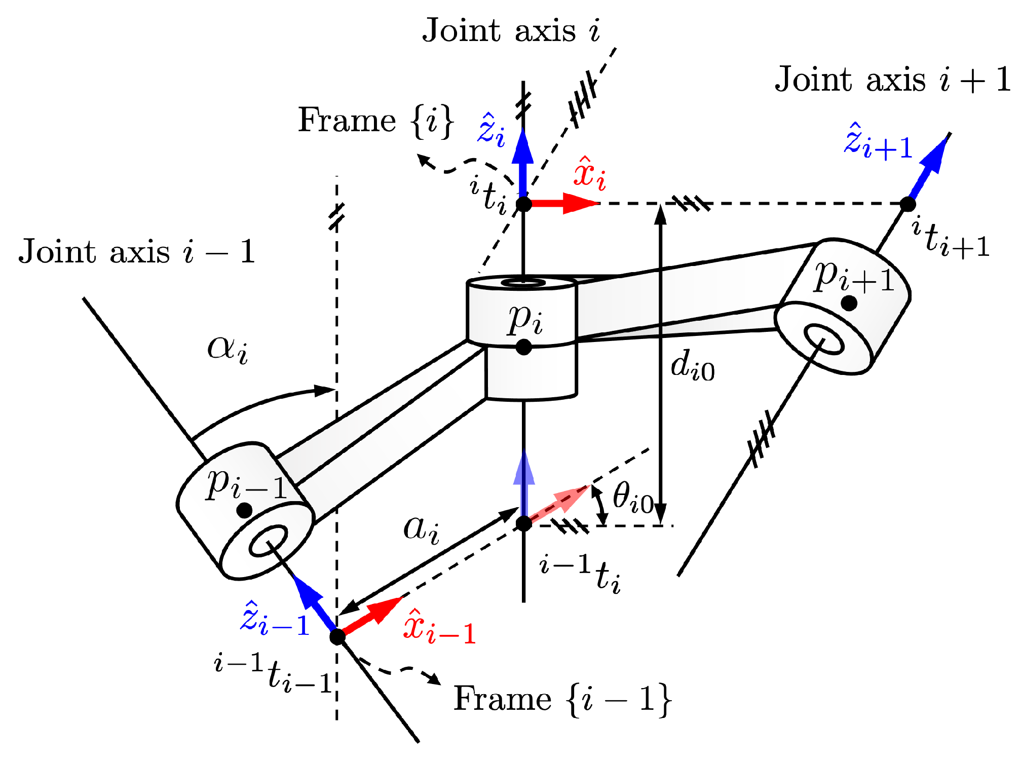
Figure 1.
Modified Denavit–Hartenberg (MDH) parameters, where denotes the point on the th joint axis, the -axis is set along the th joint axis, the -axis is determined to be a common perpendicular direction from the -axis to the -axis, and the origin of the frame denoted by is an intersection point of the -axis and the -axis. Also, four MDH parameters are denoted as , , , and .
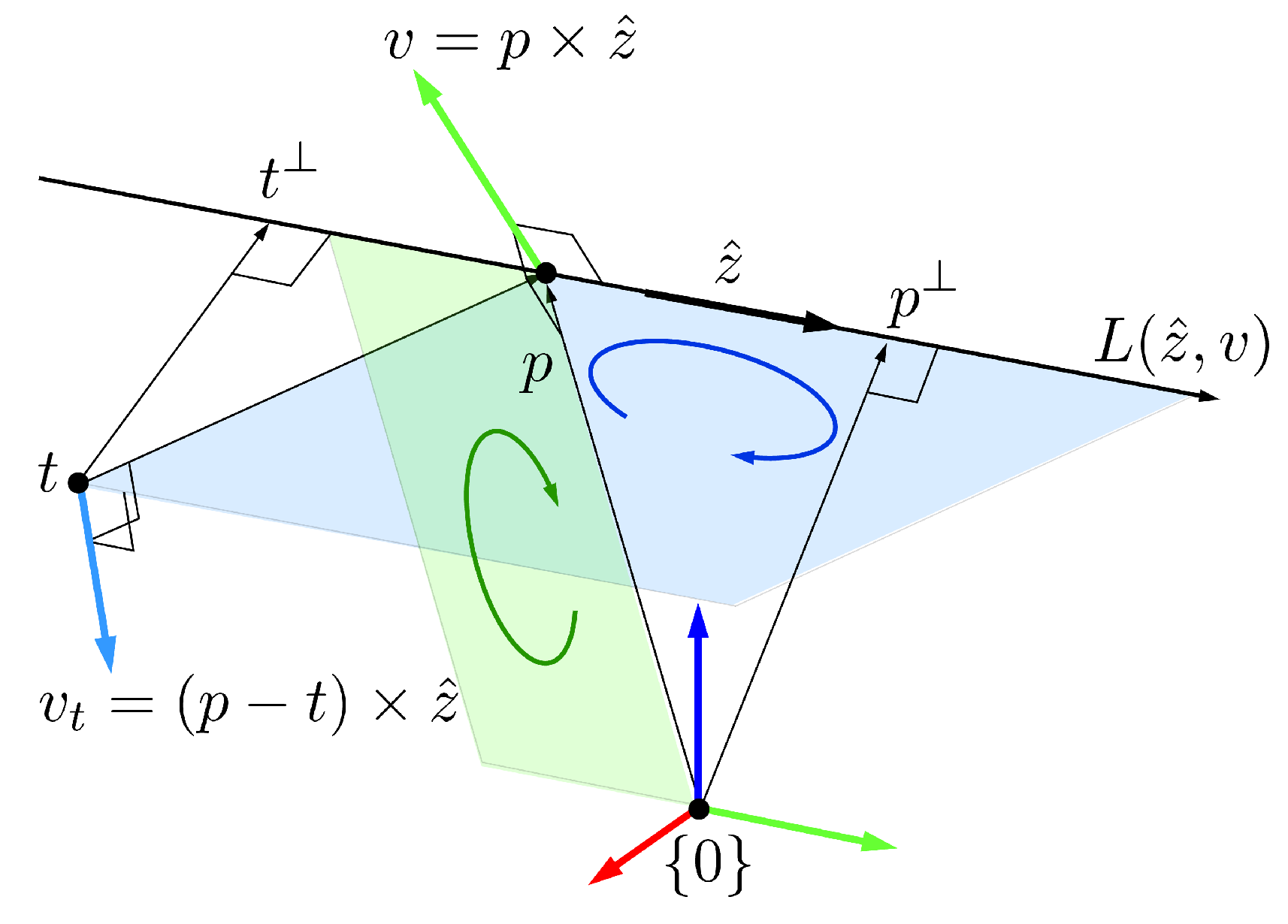
Figure 2.
Relationships between a line and a point p on the line, and between the line and a point t out of the line in three-dimensional space.
Figure 2.
Relationships between a line and a point p on the line, and between the line and a point t out of the line in three-dimensional space.
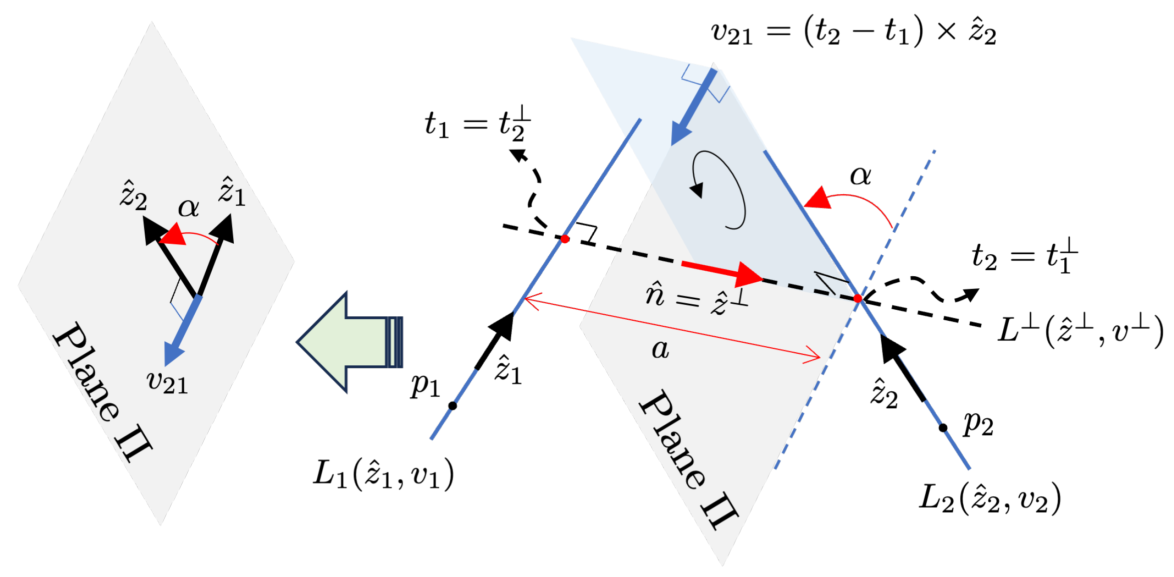
Figure 3.
Relationships between two lines and , where a is the distance between two lines, and are feet of the common perpendicular line to two lines, and is the direction vector from to .
Figure 3.
Relationships between two lines and , where a is the distance between two lines, and are feet of the common perpendicular line to two lines, and is the direction vector from to .
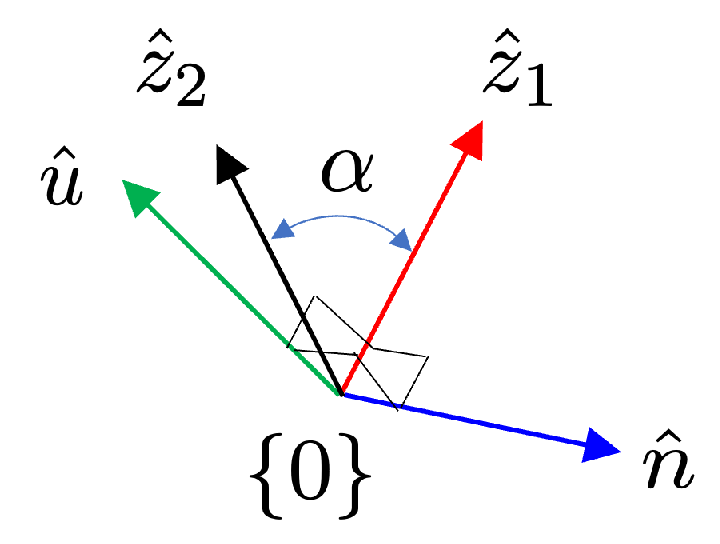
Figure 4.
The plane contains and , which is orthogonal to the common perpendicular line and parallel to ; consequently, it contains as well, where implies the twist angle of rotation from to about the common perpendicular line, and is perpendicular to .
Figure 4.
The plane contains and , which is orthogonal to the common perpendicular line and parallel to ; consequently, it contains as well, where implies the twist angle of rotation from to about the common perpendicular line, and is perpendicular to .
Figure 5.
-- coordinate frame, where lies in the - plane, and thus and for .
Figure 5.
-- coordinate frame, where lies in the - plane, and thus and for .
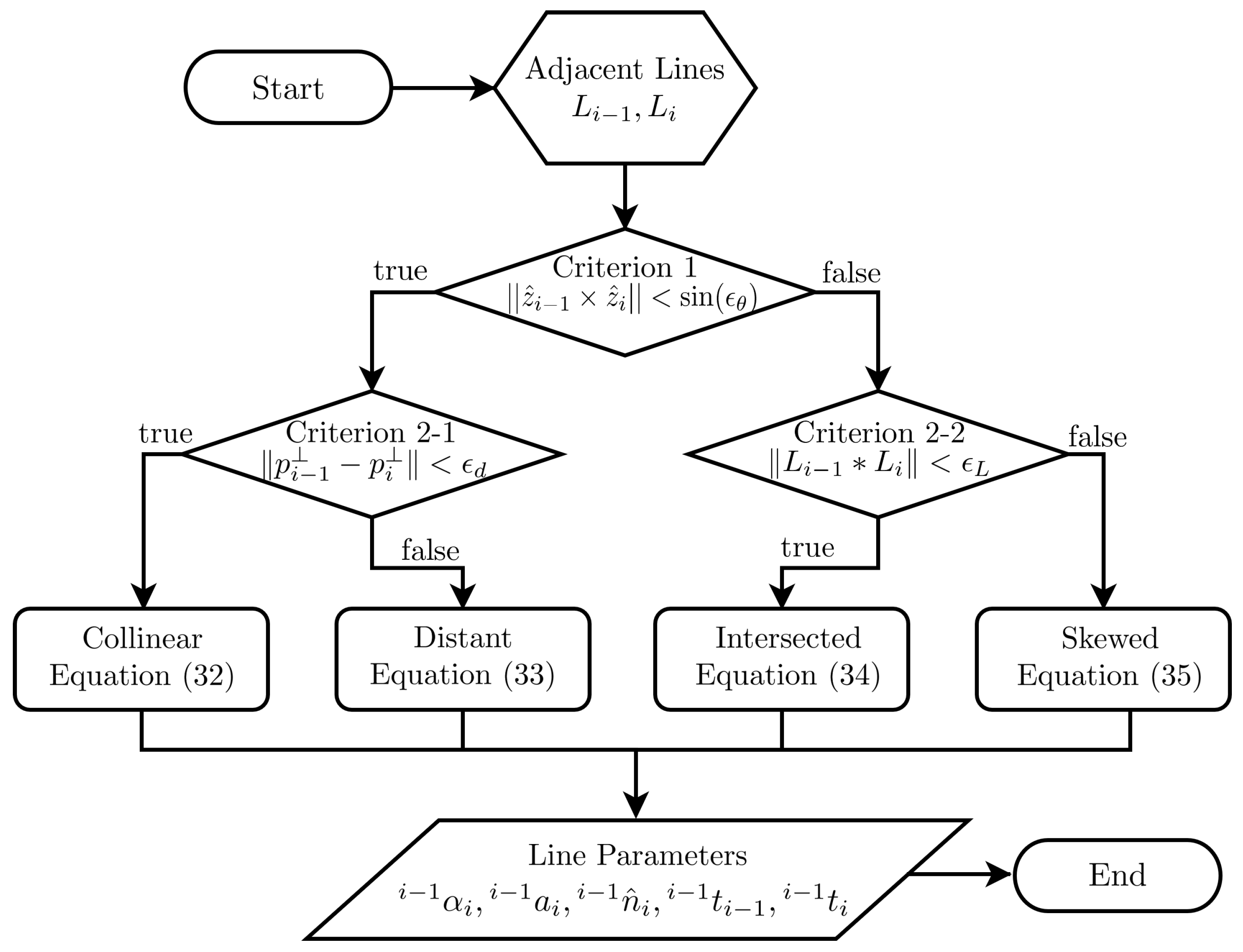
Figure 6.
Flowchart of the line geometry block . Given two input lines, and , the block uses two criteria to classify their relationship into one of the four cases: Collinear, Distant, Intersected, or Skewed. Based on the case, it returns five parameters: , , , , and .
Figure 6.
Flowchart of the line geometry block . Given two input lines, and , the block uses two criteria to classify their relationship into one of the four cases: Collinear, Distant, Intersected, or Skewed. Based on the case, it returns five parameters: , , , , and .
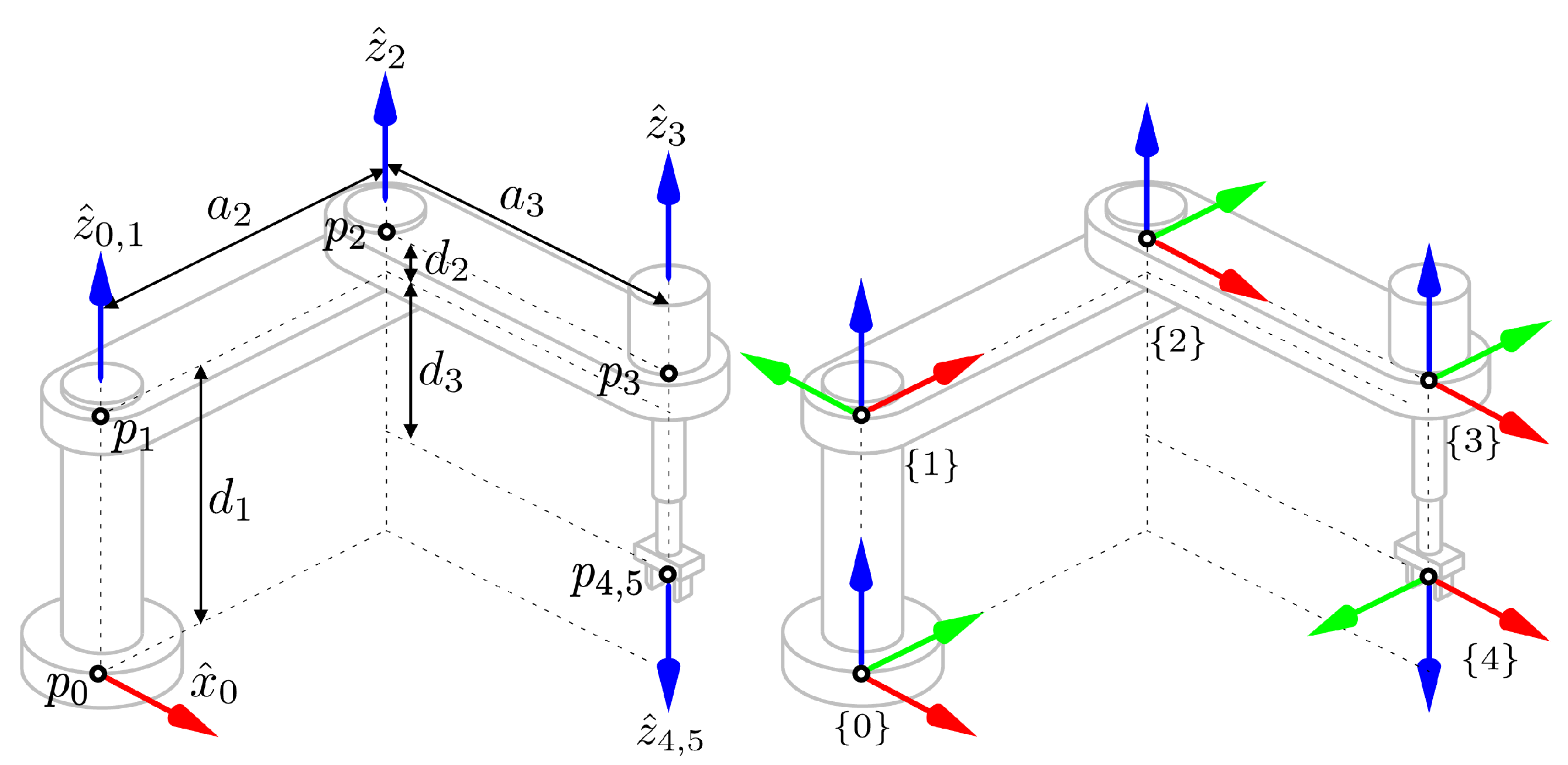
Figure 7.
The SCARA robot example, where the left side shows six line information including the base and TCF and the right side illustrates the result of MDH parameters extracted using Algorithm 1, in which the red arrow denotes the -axis, the green arrow expresses the -axis, and the blue arrow represents the -axis, respectively. In addition, the circle ∘ on the left side denotes the point , and ∘ on the right side expresses the origin of the ith frame.
Figure 8.
MDH parameters of Indy7, where the left side shows the input data regarding
and
denoted by the circle ∘, and the right side illustrates the frames obtained from the MDH parameters. Numerical data of input/output for Algorithm 1 are given in
Table 9.
Figure 8.
MDH parameters of Indy7, where the left side shows the input data regarding
and
denoted by the circle ∘, and the right side illustrates the frames obtained from the MDH parameters. Numerical data of input/output for Algorithm 1 are given in
Table 9.
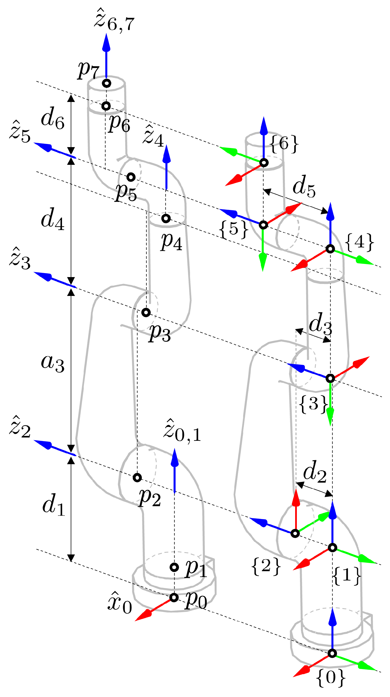
Figure 9.
MDH parameters of KUKA LBR iiwa, where the left side shows the input data regarding
and
denoted by the circle ∘, and the right side illustrates the frames obtained from the MDH parameters. Numerical data of input/output related to Algorithm 1 are given in
Table 11.
Figure 9.
MDH parameters of KUKA LBR iiwa, where the left side shows the input data regarding
and
denoted by the circle ∘, and the right side illustrates the frames obtained from the MDH parameters. Numerical data of input/output related to Algorithm 1 are given in
Table 11.
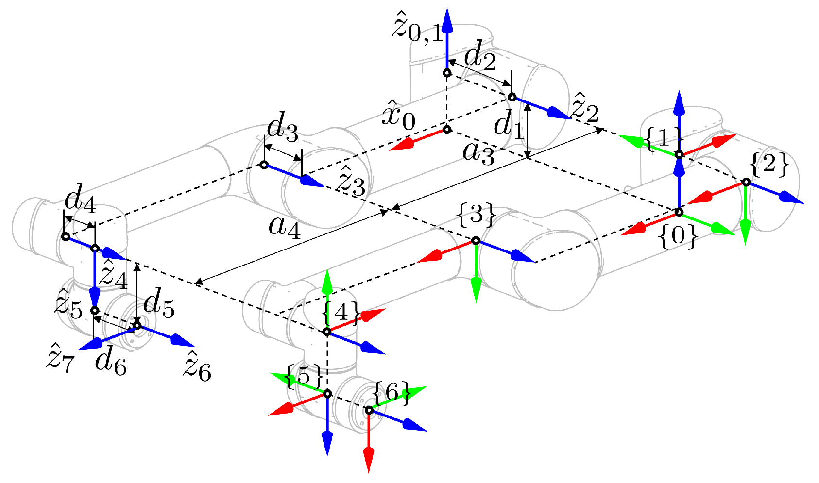
Figure 10.
MDH parameters of UR5, where the left side shows the input data regarding
and
denoted by the circle ∘, and the right side illustrates the frames obtained from the MDH parameters. Numerical data of input/output related to Algorithm 1 are given in
Table 13.
Figure 10.
MDH parameters of UR5, where the left side shows the input data regarding
and
denoted by the circle ∘, and the right side illustrates the frames obtained from the MDH parameters. Numerical data of input/output related to Algorithm 1 are given in
Table 13.
Table 1.
The generalized joint variables with MDH parameters.
Table 1.
The generalized joint variables with MDH parameters.
| Joint Type | Generalized Joint Variables () |
|---|
| Revolute (R) | |
| one-dof | |
| Prismatic (P) | |
| one-dof | |
| Helical (H) | |
| one-dof | |
| Cylindrical (RP) | |
| two-dof | |
Table 2.
MDH parameters of the Selective Compliance Assembly Robot Arm (SCARA) robot extracted when inputs are -axis, on the ith joint axis, and its moments denoted by , where outputs of Algorithm 1 are obtained as a set of -axis, link twist , link length , joint offset distance , and joint offset angle for the ith joint. Additionally, and are both feet of the common perpendicular line.
| | i | 0 | 1 | 2 | 3 | 4 | 5 |
|---|
| input | | | | | | | |
| | | | | | |
| | | | | | |
| output | | × | | | | | × |
| | | | |
| | | | |
| 0 | 0 | 0 | |
| 0 | 0.5 | 0.5 | 0 |
| 0.375 | 0.025 | 0 | 0.25 |
| | − | 0 | 0 |
Table 3.
Relations between adjacent joint axes computed from the SCARA model.
Table 3.
Relations between adjacent joint axes computed from the SCARA model.
| | b/w 0 and 1 | 1 and 2 | 2 and 3 | 3 and 4 | 4 and 5 |
|---|
| relation | collinear | distant | distant | collinear | collinear |
Table 4.
The generalized joint variables with MDH parameters for the SCARA robot.
Table 4.
The generalized joint variables with MDH parameters for the SCARA robot.
| Joints | Generalized Joint Variables () |
|---|
| 1st revolute | |
|
| 2nd revolute | |
|
| 3rd revolute | |
|
| 4th prismatic | |
|
Table 5.
Exponential coordinates , , and joint matrices for SCARA robot joints.
Table 5.
Exponential coordinates , , and joint matrices for SCARA robot joints.
| i | Joint Type | | | |
|---|
| 1 | R | | | |
| 2 | R | | | |
| 3 | R | | | |
| 4 | P | | | |
Table 6.
Comparison of nominal and perturbed URDF parameters for the SCARA robot.
Table 6.
Comparison of nominal and perturbed URDF parameters for the SCARA robot.
| Joint Pair | Orientation (Roll, Pitch, Yaw) [deg] | Position (x, y, z) [m] |
|---|
| Nominal
| Perturbed
| Nominal
| Perturbed
|
|---|
| 0–1 | (0, 0, 0) | (0, 0, 0) | (0, 0, 0.375) | (0, 0, 0) |
| 1–2 | (0, 0, 0) | (1, 1, −1) | (0, 0.5, 0.025) | (0.01, 0.51, −0.024) |
| 2–3 | (0, 0, 0) | (1, −1, 1) | (0.5, 0, 0) | (0.51, −0.01, 0.01) |
| 3–4 | (0, 0, 0) | (−1, −1, −1) | (0, 0, −0.25) | (−0.01, −0.01, −0.29) |
| 4–5 | (0, 0, 0) | (0, 0, 0) | (0, 0, 0) | (0, 0, 0) |
Table 7.
Extracted MDH parameters from the perturbed SCARA robot, using small positive threshold .
Table 7.
Extracted MDH parameters from the perturbed SCARA robot, using small positive threshold .
| Parameter | Joint 1 | Joint 2 | Joint 3 | Joint 4 |
|---|
| [rad] | 0.0000 | 0.0247 | 0.0247 | 0.0247 |
| [m] | 0.0000 | 0.3614 | 0.3739 | 0.0141 |
| [m] | 14.8930 | −0.5166 | −14.3041 | −0.0100 |
| [rad] | 0.7678 | −1.5533 | −1.5883 | 0.0000 |
Table 8.
Relations between adjacent joint axes computed from the perturbed URDF model.
Table 8.
Relations between adjacent joint axes computed from the perturbed URDF model.
| | b/w 0 and 1 | 1 and 2 | 2 and 3 | 3 and 4 | 4 and 5 |
|---|
| Relation | collinear | skewed | skewed | skewed | collinear |
Table 9.
Indy7, where upper part and lower part imply the input data to the Algorithm 1 and the output yielded from the algorithm, respectively.
Table 9.
Indy7, where upper part and lower part imply the input data to the Algorithm 1 and the output yielded from the algorithm, respectively.
| | i | 0 | 1 | 2 | 3 | 4 | 5 | 6 | 7 |
|---|
| input | | | | | | | | | |
| | | | | | | | |
| | | | | | | | |
| | i | 0 | 1 | 2 | 3 | 4 | 5 | 6 | 7 |
| output | | × | | | | | | | × |
| | | | | | |
| | | | | | |
| output | | | 0 | | 0 | | | | |
| | 0 | 0 | | 0 | 0 | 0 | |
| | | | | | | | |
| | 0 | | | | | 0 | |
Table 10.
Relations between adjacent joint axes computed from the Indy7 model.
Table 10.
Relations between adjacent joint axes computed from the Indy7 model.
| | b/w 0 and 1 | 1 and 2 | 2 and 3 | 3 and 4 |
|---|
| relation | collinear | intersected | distant | intersected |
| | 4 and 5 | 5 and 6 | 6 and 7 | |
| relation | intersected | intersected | collinear | |
Table 11.
KUKA LBR iiwa, where upper part and lower part imply the input data to the Algorithm 1 and the output yielded from the algorithm, respectively.
Table 11.
KUKA LBR iiwa, where upper part and lower part imply the input data to the Algorithm 1 and the output yielded from the algorithm, respectively.
| | i | 0 | 1 | 2 | 3 | 4 | 5 | 6 | 7 | 8 |
|---|
| input | | | | | | | | | | |
| | | | | | | | | |
| | | | | | | | | |
| output | | × | | | | | | | | × |
| | | | | | | |
| | | | | | | |
| 0 | | | | | | |
| 0 | 0 | 0 | 0 | 0 | 0 | 0 |
| | 0 | | 0 | | 0 | |
| | | 0 | | 0 | | 0 |
Table 12.
Relations between adjacent joint axes computed from the KUKA LBR iiwa model.
Table 12.
Relations between adjacent joint axes computed from the KUKA LBR iiwa model.
| | b/w 0 and 1 | 1 and 2 | 2 and 3 | 3 and 4 |
|---|
| relation | collinear | intersected | intersected | intersected |
| | 4 and 5 | 5 and 6 | 6 and 7 | 7 and 8 |
| relation | intersected | intersected | intersected | collinear |
Table 13.
UR5, where the upper part and lower part imply the input data to the Algorithm 1 and the output yielded from the algorithm, respectively.
Table 13.
UR5, where the upper part and lower part imply the input data to the Algorithm 1 and the output yielded from the algorithm, respectively.
| | i | 0 | 1 | 2 | 3 | 4 | 5 | 6 | 7 |
|---|
| input | | | | | | | | | |
| | | | | | | | |
| | | | | | | | |
| output | | × | | | | | | | × |
| | | | | | |
| | | | | | |
| 0 | | 0 | 0 | | |
| 0 | 0 | | | 0 | 0 |
| | | | | | |
| | | 0 | | | |
Table 14.
Relations between adjacent joint axes computed from the UR5 model.
Table 14.
Relations between adjacent joint axes computed from the UR5 model.
| | b/w 0 and 1 | 1 and 2 | 2 and 3 | 3 and 4 |
|---|
| relation | collinear | intersected | distant | distant |
| | 4 and 5 | 5 and 6 | 6 and 7 | |
| relation | intersected | intersected | intersected | |


