Reproducibility Assessment of Zirconia-Based Ceramics Fabricated out of Nanopowders by Electroconsolidation Method

Featured Application

the results of this work can be useful in any application of zirconia-based ceramics, especially when considering various sintering methods.

Abstract

The repeatability of the material properties is required to ensure the proper performance of the engineered systems that are constructed using these materials. In this paper, an analysis of the sintered ceria-stabilized zirconia is presented. This material exhibited high mechanical properties, due to the mechanism of strengthening via phase transition. The reproducibility was assessed for the material made out of a starting powder produced by fluoride salt precipitation. To fabricate specimens, a novel electroconsolidation method was used, ensuring a high heating rate, relatively low sintering temperatures, and short holding time. Weibull analysis was performed considering the bending strength of specimens and their microhardness. The obtained values of both shape parameter m and scale parameter σ₀ indicated that the ZrO₂ stabilized with 5 wt.% CeO₂ samples exhibited low variability of strength and hardness. The experimental evidence and statistical analysis reveal an influence of the m-phase, which has lower symmetry and therefore its addition makes ceramic weaker and softer. Furthermore, its progressive replacement by the t-phase, which has higher symmetry, makes ceramic both harder and stronger. Reducing the mol% increases the risk of the appearance of the highest addition of the monoclinic phase; increasing it is unfavorable from the point of view of the sintering process. Statistical and manufacturing evidence suggests that the choice of 5%/mol is optimal.

1. Introduction

Ceramic materials based on zirconia (zirconium oxide, ZrO₂) attract the attention of researchers and industry due to their unique physical and chemical properties, such as high flexural strength, hardness, corrosion resistance, and thermal stability [1]. Due to these advantageous properties, zirconia is considered one of the vital materials for engineering, tools, dental, or orthopedic applications [2,3,4]. Zirconia-based ceramics serve as a catalyst and are used as a material for solid fuel cells due to their unique characteristics [5]. Zirconia exhibits superior thermal resistance with a melting temperature ca. 2700 °C, which makes it a more effective material for isolation layers than glass or quartz fibers [6].

Pure zirconia, under low-pressure conditions, exists in three distinct crystalline phases: monoclinic (m-ZrO₂, P21c, stable to 1170 °C), tetragonal (t-ZrO₂, P42/nmc, stable 1170–2370 °C) and cubic (c-ZrO₂, Fm3m, stable 2370–2900 °C). In the presence of pressure, a primary phase transition from monoclinic to orthorhombic phase is observed at 3–11 GPa [7,8,9] (brookit phase, either Pbcm or Pbca), with a secondary transition occurring at 9–15 GPa [8] (Pnam, isostructural to cotunnite). The rutile phase, which is theoretically predicted and should be more stable than the monoclinic phase, has not yet been observed in experimental studies. Furthermore, zirconia has a polycrystalline biphasic structure [10]. At elevated temperatures, pure zirconia has a tetragonal structure t-ZrO₂, and a monoclinic phase m-ZrO₂ at room temperature, but two phases, t-ZrO₂ and m-ZrO₂, can coexist, e.g., in a matrix. Since the tetragonal phase is unstable, it is usually stabilized with yttria, making up a hard, tough structural ceramic feasible for the high-temperature applications, e.g., in jet engines [11]. Recently, cerium has been considered as an attractive alternative to yttria for stabilizing zirconia, due to its higher toughness compared with yttria-stabilized zirconia, even though CeO₂ ceramics exhibited relatively low strength [12]. Some researchers pointed out that zirconia with Y₂O₃ has better mechanical properties, but it suffers from the disadvantage of degrading at low temperature. Experimental evidence suggests that CeO₂-doped zirconia is more stable [13]. Due to higher mobility of grain boundaries, the grain size after sintering is larger, making challenging the fabrication of completely dense ceria-stabilized zirconia ceramics with fine grains [14].

In recent years, significant attention has been paid to nanostructured ceramics, because reducing the grain size results in increased hardness and fracture resistance of the ceramic. Indeed, the ZrO₂ nanopowders exhibit enhanced mechanical and functional characteristics compared to coarse-grained materials [15]. One of the most promising methods for obtaining such nanopowders is an electrospray deposition technique [16]. However, for successful industrial application, it is necessary to ensure the reproducibility of the properties of the obtained materials. It is widely known that the particle size distribution of the initial powder plays a crucial role in further compaction and thus has an effect on the properties of the sintered material [17]. The utilization of nanopowders is contingent upon the procurement of substantial quantities of materials that are characterized by their reproducible quality.

Research has demonstrated that by optimizing the conditions of electrospray deposition, high reproducibility of the structure and properties of nanopowders can be achieved [18]. In particular, under certain process parameters, it is possible to obtain particles with a narrow size distribution, ensuring stable mechanical properties of the sintered ceramic products. Controlling the phase composition is an important factor, as well, since the presence of different phases (tetragonal, monoclinic, cubic) affects the mechanical properties and stability of the material. Optimization can be performed by minimizing or maximizing some objective functions, such as stiffness, mass, etc. [19].

Similarly, it is crucial to keep repeatable processing conditions to fabricate sintered ceramics with reproducible properties [20]. However, on the microscopic scale, random variation in strength may occur due to the randomly distributed microdefects that are common in quasi-brittle materials in terms of spatial arrangement, orientation, size, and shape [21]. Thus, it is convenient to estimate the likelihood of the crack propagation as a measure of the material’s fracture resistance.

Weibull analysis (WA) is a statistical analysis widely used in reliability applications to identify failure modes [22,23]. It is an effective technique for obtaining material reliability results at a moderately low rate, with the reliability of the material or component being assured [24]. The Weibull modulus of aggregate tensile strength distribution is correlated to the heterogeneity of particle binding force distribution within the aggregate. The sensitivity of the Weibull modulus to detect small differences in the internal structure of aggregates depends on the standardization of aggregate shape and sphericity. The Weibull modulus is highly sensitive to the heterogeneity of particle binding force distribution within the aggregate. An increase in the heterogeneity of the particle binding force distribution results in a linear decrease in the Weibull modulus of the aggregate tensile strength [25]. The two-parameter (2P) Weibull distribution function, based on scale and shape parameters, is the most commonly used statistical model for characterizing the strength of modern ceramics [26]. The primary benefit of Weibull analysis is that it facilitates the analysis of failures, even with limited data samples. It also provides a graphical representation of the individual failure modes that can be readily interpreted, as well as an indication of the failure physics (based on the slope of the distribution).

The probabilistic strength description parameters obtained from the Weibull distribution should match the observed material microstructure. Indeed, the Weibull distribution has been successfully used to describe the fracture strength of microscale materials such as silicon and composite-reinforcing fibers and has been used to a lesser extent for thin films, nanotubes/wires, and 2D materials [27].

The Weibull distribution has been extensively utilized in the fields of reliability analysis and durability testing of a wide range of industrial products. This distribution has been found to provide an effective representation of the degradation trajectory or the form of material failure. Additionally, it has been demonstrated to assist in addressing the challenges posed by uncertainty and randomness in damage caused by internal defects in brittle materials [28].

Despite significant success reported on the zirconia ceramics research, the mechanisms of its performance are not yet fully established. For instance, it is necessary to ascertain the details of the microstructural transformation and stability-dependent factors of t:m phase proportions, surface chemistry, and porosity, as well as properties dependent on the applied load. The research described in this paper contributes to fill some of these gaps. The reproducibility of the properties of ceramics sintered out of ZrO₂ nanopowders obtained by electrospray deposition is a key factor for the successful improvement of the electroconsolidation device prototype, designed for further investigations. The objective of this paper was to analyze the distribution of properties, both for synthesis and processing parameters, using the Weibull model. The powder characteristics, a description of the sintering process, results of strength and hardness measurements, and most importantly, their statistical analysis enabled an assessment of the degree of material reproducibility.

2. Materials and Methods

2.1. Powder Preparation

The synthesis of zirconium nanopowders was accomplished through the utilization of the fluoride salt decomposition method, a process that has been extensively delineated in [29]. However, the precipitation process was performed at three different temperatures, 20 °C, 50 °C, and 80 °C, and the ratio of metallic zirconium to polyvinyl alcohol (PVC) was varied, as follows: m(Zr):m(PVC) was 1:0.1, 1:0.5, and 1:1.

The as-obtained substance was filtered and washed using distilled water, and then it was dried for 48 h at 20 °C. Then, the powder was heated up to 800 °C, applying the heating rate ca. 100 °C/h, and held for 4 h. Afterwards, the zirconia powder was cooled down to room temperature. To obtain homogeneity of the nanopowder, it was mixed with the planetary micro mill Pulverisette 7 (Fritsch GmbH, Idar-Oberstein, Germany), shown in Figure 1.

The use of cerium oxide was instrumental in the stabilization of the zirconium powder. Nanopowder CeO₂ was purchased from Nanografi Nano Technology (Ankara, Turkey). It was gradually added to the blend and mixed until homogeneity. The amount of added cerium oxide was calculated to obtain 5 mol% proportion in the zirconia powder. The blend was prepared by dry method and with application of isopropyl alcohol. The mixing process lasted for 2 h with planetary disk rotational speed of 160 rpm.

The degree of stabilization is dependent on the particular stabilizer type, its calcination temperature, and quantity of contaminations [30]. The reports on Ce-stabilized zirconia with CeO₂ content from 8 mol% up to 16 mol% pointed out the poor sinterability of these materials that required a prolonged heating, which, in turn, resulted in higher grain growth [31]. Thus, it was decided to perform experiments with a reduced ceria proportion of 5 mol%. It was also noted that during the synthesis process, this composition exhibited higher thermodynamic stability and lower structural anisotropy.

2.2. Electroconsolidation Method

A method for fabrication of sintered specimens was a sort of powder metallurgy technique, a modified spark plasma sintering (SPS) [32], or electric field activated sintering technology (E-FAST) [33] method. The main idea and apparatus used for electroconsolidation are presented in detail elsewhere [34]. The sole source of heat in this modified SPS process was high electrical current, reaching ca. 5000 A. Unlike a typical SPS pulsed direct current [35], an alternating current is used in the electroconsolidation technique.

The electroconsolidation apparatus is shown in Figure 2. Figure 2a presents the device, specifying its main units. In Figure 2b, graphite mold is presented, shaped for the fabrication of cylindrical specimens of diameter 11 mm and height 5 mm.

The synthesized nanopowders ZrO₂–5 wt.% CeO₂ were sintered at temperature 1400 °C under mechanical pressure 45 MPa; holding time was 2 min.

2.3. Materials Characterization

Scanning electron microscopy (SEM) was utilized for the purpose of sample analysis. It provides information about the surface topography and composition of the sample. The experimental procedure was performed using NovaNanoSEM 450 microscope (FEI Europe B.V., Eindhoven, The Netherland). Microscopic images were taken using the following detectors: TLD (Through the Lens Detector, topographic contrast) and CBS (Circular Backscatter Detector, material contrast) at accelerating voltages of 5 kV and 15 kV, respectively. Distance to sample (Working Distance, WD) was 4 mm for TLD detector and 5 mm for CBS.

To determine the specific surface area of the initial powders, the BET (Brunauer–Emmett–Teller) method was used, with nitrogen (N₂) being the widely accepted standard adsorptive [36]. For that purpose, the device BELSORP-mini II produced by BEL Japan, Inc. (Toyonaka, Japan) was employed. All samples were measured by degassing at 100 °C for 3 h.

The elemental microanalysis was performed using Octane energy dispersive X-ray detector (AMETEK, Inc., Berwyn, PA, USA). The applied Octane Elect Plus silicon drift detector (SDD) was equipped with a chip of 30 mm² area. The X-ray diffraction analysis (XRD) was performed using Philips X’Pert Pro Materials Powder Diffractometer (Philips Analytical, now PANalytical, Almelo, The Netherlands) in order to evaluate the phase composition of the zirconia powder. The CuKα radiation source was used in XRD, with an anode voltage of 45 kV and a current of 40 mA.

The strength analysis was based on the results of three-point bending strength tests and Vickers hardness measurements. For that purpose, Bending Testing Machine DELTA 5–200 was used (Form+Test Seidner&Co. GmbH, Riedlingen, Germany). For the hardness, the tester type FALCON 400G2 produced by Innovatest (Maastricht, The Netherland) was applied.

2.4. Weibull Analysis

To ascertain the reliability of the samples, a Weibull analysis was undertaken. The Weibull distribution is a type of statistical continuous probability distribution; a flexible model that is frequently used to approximate the normal, Rayleigh, or exponential distribution. It can be used to model data exhibiting right-skewed, left-skewed, or symmetric properties.

This versatility renders it a suitable model for assessing reliability. The Weibull distribution has been demonstrated to be an effective extreme value distribution for the purpose of predicting the occurrence of extreme phenomena. Therefore, it is widely used to describe the probabilistic failure behavior of materials. In general, the Weibull distribution is defined either by its probability density function or cumulative distribution function. The original Weibull model is three-parametric with shape indicating whether the failure rate is increasing, decreasing, or constant over time, scale that stretches or compresses the distribution, and threshold that shifts the distribution along the X-axis. The latter is optional and neglected in the 2D model. The parameters of the Weibull distribution can be determined analytically, employing either least squares (rank linear or non-linear regression) or maximum likelihood estimation (MLE). In this study, the former approach was used.

Thanks to linearization procedure, the Weibull method can theoretically work with extremely small samples, even with two or three failures. In order to achieve statistical relevance, it is necessary to increase the size of the sample. Usually, Weibull analysis requires at least 30 samples (the central limit theorem requirement). For a distribution that differs significantly from normal, it may be necessary to use as many as about 30 samples. However, it is important to note that, given the wide array of probability distributions that exist, this criterion may not be universally applicable. Therefore, this rule can be revised under certain prerequisites [37,38].

However, relatively small dispersion of the values was noted, so based on [39], it was found acceptable to reduce the number of samples down to 15. The performed Shapiro–Wilk test did not show a significant departure from normality, with parameters W(15) = 0.9445, p = 0.4428 for bending strength and W(15) = 0.9447, p = 0.4455 for hardness. Since p-values in both cases were larger than α, we accepted the H₀ hypothesis, assuming that the data were normally distributed.

3. Results and Discussion

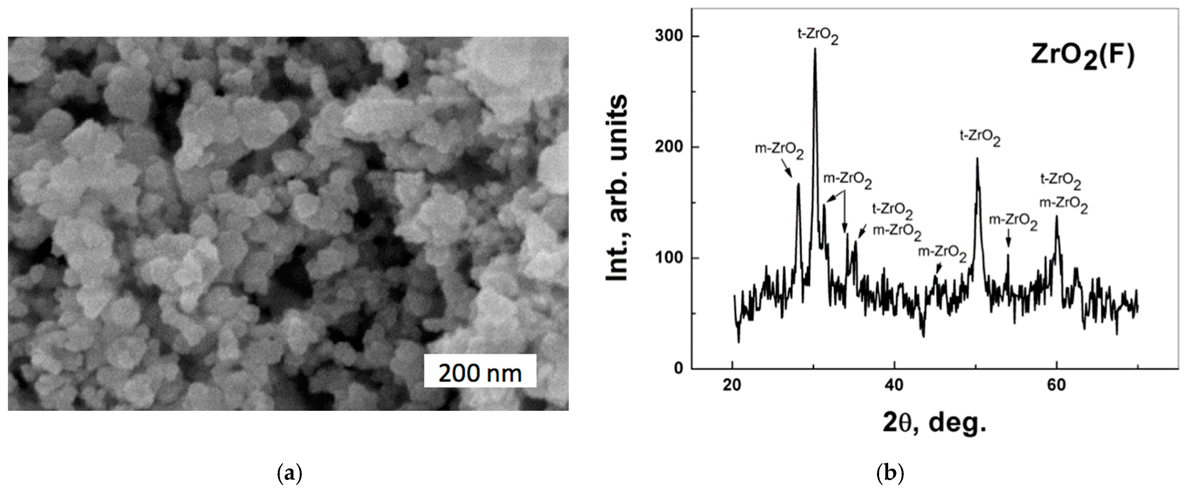
3.1. Characterization of the Initial Powder

The powder synthesized via the precipitation route described in Section 2.1 is shown in Figure 3. In particular, the SEM image is presented in Figure 3a, and the XRD diagram is provided in Figure 3b.

The homogeneity of powder morphology can be noted from the SEM image (Figure 3a). It can be expected that the highly uniform particle size distribution contributed to the improved sinterability of the zirconia powder. The XRD diagram (Figure 3b) exhibits the presence of both phases, tetragonal t-ZrO₂ and monoclinic m-ZrO₂. Thus, the sample under investigation exhibits a biphasic structure.

Figure 4 shows the BET (Brunauer–Emmett–Teller) isotherm of the initial powder. Its specific surface area a_sBET was found to be 6.3. Compared to the powder obtained by other means, this powder was of significantly higher quality. The specific surface area for the second powdered sample was a_sBET = 3.7, and this powder was of poor quality and thus excluded from further studies.

The hysteresis shown in Figure 4a belongs to a Type IVa isotherm, according to the classification provided in [40]. Its two branches represent adsorption and desorption associated with capillary condensation. Capillary condensation typically occurs in granular or porous media and can strongly alter the properties of the materials. Its presence suggests the van der Waals interactions between the molecules assemble crystals to create atomic-scale capillaries in the condensed state.

Although the final saturation plateau is very small, this indicates a mesoporous material. The increase in mesoporosity can be attributable to the augmented number of grain boundaries, consequent to the formation of phase-separated nanocomposites.

For nitrogen, adsorption took place in cylindrical pores at 77 K, and hysteresis started to occur for pores above 4 nm in width. The pore volume versus pore diameter shown in Figure 4b reveals three local extremes at diameter values of about 2.5, 7.5, and 11 nm.

The observed morphology and the results of the BET analysis indicated that the initial powder exhibited good sinterability.

3.2. Microstructural Analysis of the Sintered Specimens

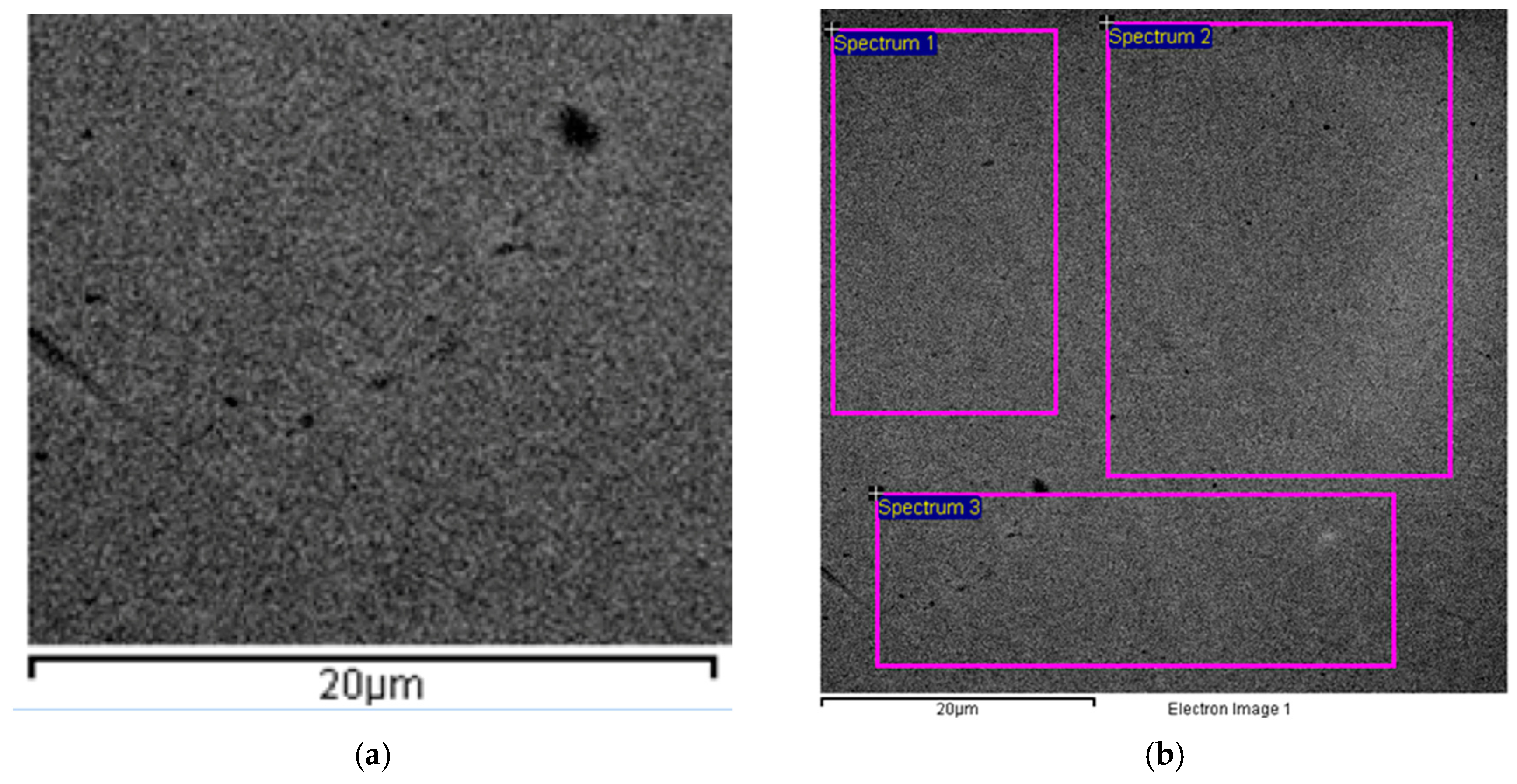
The microstructure of a sintered sample is shown in Figure 5. The structure of the specimen was found to be homogeneous with several small dark inclusions of distinguishable size. The three areas selected for the elemental analysis are illustrated in Figure 5b, and the numerical data are listed in

Table 1. Elemental analysis of sintered ZrO₂–5wt.% CeO₂ specimen.

Spectrum No.	O, wt.%	Ce, wt.%	Zr, wt.%
Spectrum 1	30.5	5.39	64.1
Spectrum 2	30.8	4.99	64.2
Spectrum 3	31.9	4.27	64.8

.

The data in Table 1 suggest that some non-uniformity of ceria distribution in the zirconia matrix took place. However, its scale does not threaten the strength characteristics of the sintered material. From the perspective of fracture toughness, the proportion of tetragonal to monoclinic zirconia appeared more important. Overall, the t-ZrO₂ phase constituted ca. 95%, while the content m-ZrO₂ phase was ca. 5% in the sintered specimen. An increase in the monoclinic phase content upon cooling of zirconia sintered at temperatures higher than 1400 °C was reported in [41], which should not be expected in the present experiments with the zirconia sintered at 1400 °C. Thus, the negative effect of the monoclinic phase could be considered negligible.

The presence of the different phases (i.e., monoclinic, tetrahedral, and cubic) is evidenced in the experimental studies. The histogram shown in Figure 6 provides a concise overview of these data. The horizontal axis shows the mol% value, while the Y-axis is utilized to demonstrate the number of mentions of these structures in the literature.

When the mol% of CeO₂ in a given composite falls between 10% and 80%, the existence of the composite in various phases has been reported. The higher CeO₂ content, the higher the symmetry (for mol% < 8% formulation, it is typically monoclinic, 8 < mol% < 75% tetrahedral, or cubic and mol% > 75% cubic). The nanopowders with mol% equal to 10, 25, 50, and 75% exhibit tetrahedral symmetry, while with mol% equal to 90% exhibits cubic symmetry. Consequently, elevated mol% is associated with higher symmetry.

The addition of CeO₂ results in a significant enhancement of the stability, high-temperature resistance, and mechanical properties of ZrO₂. In contrast, the higher amounts of CeO₂ enhance the mobility of grain boundaries and increase the grain size following sintering. Therefore, the CeO₂ addition should be minimized. As demonstrated in Figure 6, at low molar percentage values (below 8 mol%), the m-phase has thus far been achieved. The electroconsolidation method outlined in this study facilitates the production of a t-phase composite comprising only 5 mol% of CeO₂, a distinctive feature.

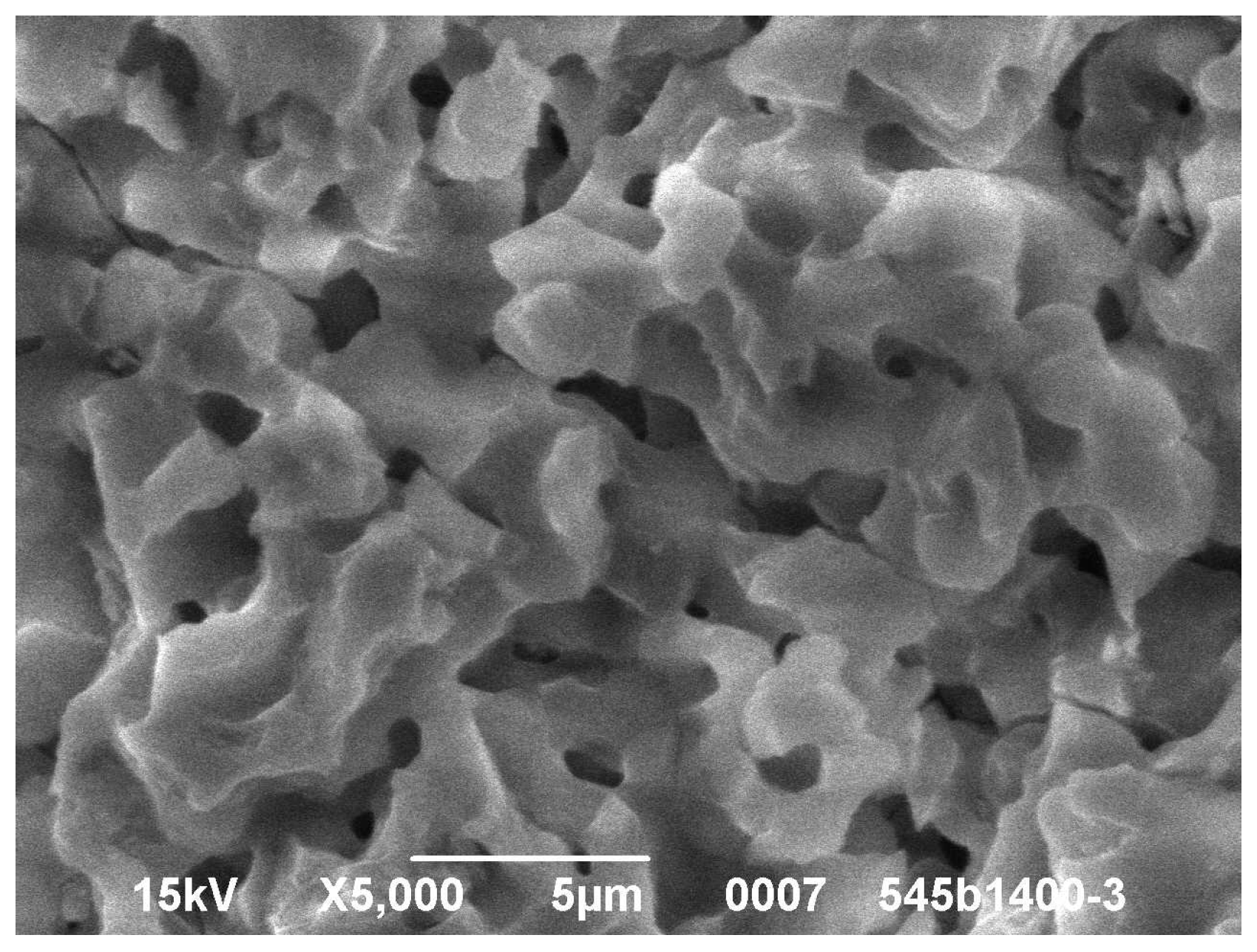
3.3. Strength Analysis

In Figure 7, there is an SEM image of a sintered sample fracture surface presented. It can be seen that after sintering, the grain size of around 1 μm was partially retained.

The destruction of grains observed in Figure 6 is predominantly transcrystalline, which indicates the strength of inter-grain boundaries. The bending strength σ_b of the specimen under three-point bending conditions was determined according to the following formula:

$${\sigma }_b={\displaystyle \frac{3Fl}{2b{h}^2}}$$

(1)

where F is the force value at the moment of separation of the sample into parts, N; l is the length of the sample, mm; b is the width of the sample, mm; h is the thickness of the sample in the parallel direction to the force applied to the sample, mm.

Different brittle materials experience rupture at different maximum tensile stresses. Statistically, the brittle fracture is dependent on the weakest element in the material’s volume. According to the two-parameter Weibull distribution, the probability of failure P_f at a given the stress value, σ, is defined as follows [42,43]:

$$P_f=1-\mathrm{e}\mathrm{x}\mathrm{p}\left[-{\left({\displaystyle \frac{\sigma }{{\sigma }_0}}\right)}^m\right]$$

(2)

where m is the shape parameter of the Weibull distribution; σ is the actual inner stress under the applied force, MPa; and σ₀ denotes the scale parameter, MPa. (The threshold value, below which no specimen is expected to fail, is neglected).

To estimate the the Weibull parameters, Equation (1) is twice logarithmed and reduced to a linear form, as follows:

$$\ln \left(\ln {\left(1-P_f\right)}^{-1}\right)=m\mathrm{l}\mathrm{n}\left(\sigma \right)-m\mathrm{l}\mathrm{n}\left({\sigma }_0\right).$$

(3)

The shape and scale parameters, m and σ₀, respectively, are obtained from Equation (3) by the least squares method. The density of fracture probability f dependent on the value of σ₀ is described by the equation, as follows:

$$f\left(\sigma \right)={\displaystyle \frac{m}{{\sigma }_0}}{\left({\displaystyle \frac{\sigma }{{\sigma }_0}}\right)}^{m-1}\mathrm{e}\mathrm{x}\mathrm{p}\left[-{\left({\displaystyle \frac{\sigma }{{\sigma }_0}}\right)}^m\right]$$

(4)

To perform the calculations, the entered experimental data are ordered in ascending order, and for each i-th value, the empirical probability function P_exp(i) is determined according to the following formula:

$$P_{exp}\left(i\right)={\displaystyle \frac{i-0.5}{N}},$$

(5)

where N is the number of tested samples.

The results of the tensile strength measurement and of related calculations are collected in

Table 2. Bending strength σ = σ_f and the probability of failure P_f for the sintered samples of ZrO₂–5 wt.% CeO₂.

Experiment No.	σf, MPa	ln(ln(1 − Pf)−1)
1	370 ± 3	–3.218
2	390 ± 3	–2.355
3	400 ± 3	–2.068
4	420 ± 5	–1.349
5	430 ± 5	–1.061
6	440 ± 5	–0.630
7	446 ± 5	–0.486
8	450 ± 5	–0.342
9	454 ± 5	–0.198
10	460 ± 5	–0.054
11	476 ± 5	0.377
12	480 ± 5	0.521
13	484 ± 5	0.665
14	490 ± 5	0.809
15	494 ± 5	0.953

.

Using the obtained data, the Weibull graph, the so-called Weibull probability plot, was plotted and is presented in Figure 7. The values calculated from the experimental data were fitted using a linear equation, as follows:

y = a₀x − a₁

(6)

where the parameters a₀ and a₁ were determined using the least squares method. The Weibull modulus m corresponds to the parameter a₀.

The scale parameter σ₀ is related to both a₀ and a₁ according to the following relation:

$${\sigma }_0=\mathrm{e}\mathrm{x}\mathrm{p}\left({\displaystyle \frac{a_1}{a_0}}\right)$$

(7)

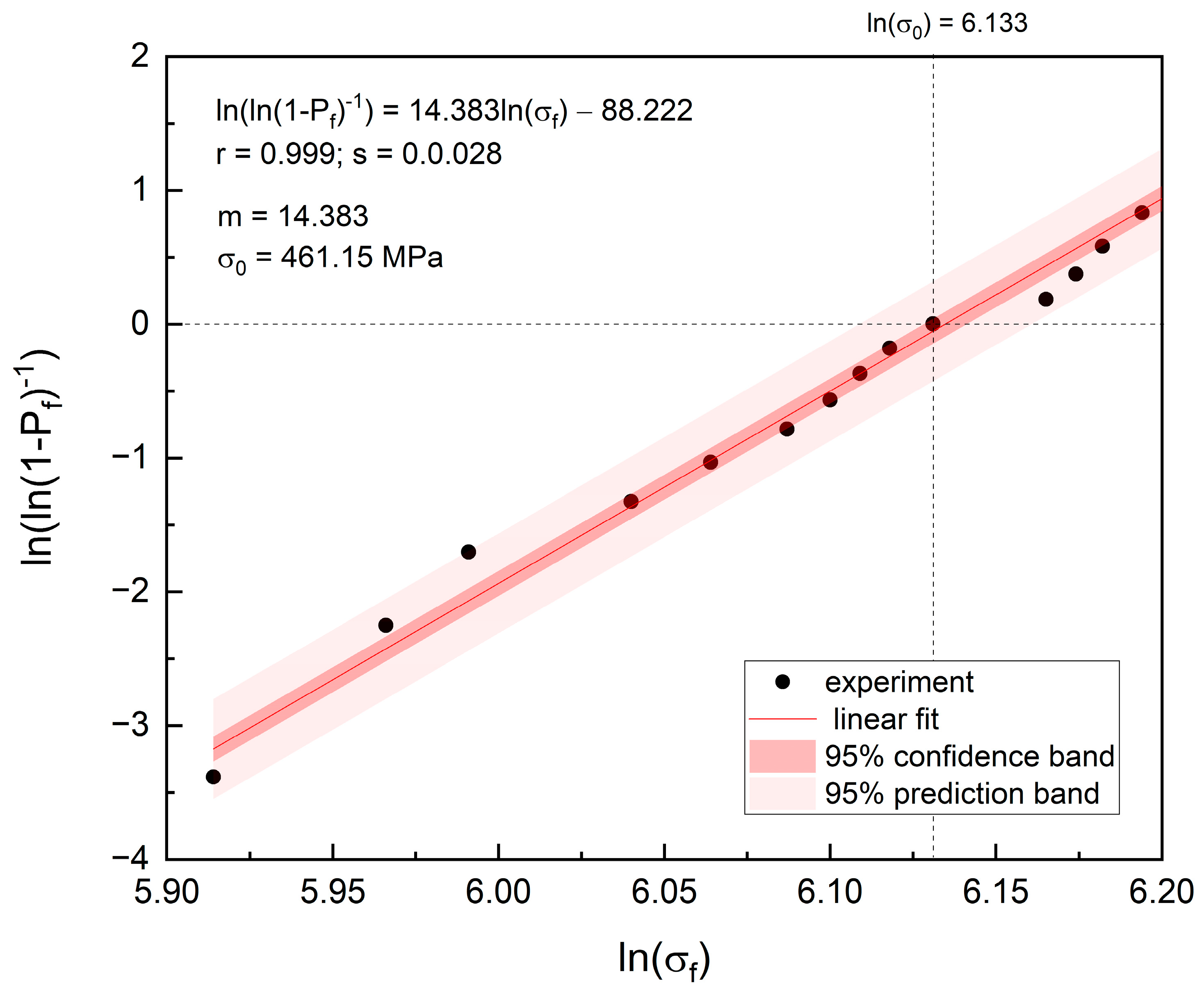
Figure 8 shows a Weibull graph, where y = ln(ln(1 − P_f)⁻¹) represents the double logarithmic transformation of the cumulative probability of failure and x = ln(σ) describes the natural logarithm of the failure bending stress. The black dots correspond to the experimental data points. The linear regression model, fitted to the data points, yielded parameters describing the Weibull distribution listed in

Table 3. The results of the parameter fitting for the best-fit formulation, along with the derived Weibull distribution parameters.

Fitting Parameters		Statistics of the Fit			Weibull Distribution Parameters
a0	a1	r	s	Reduced χ2	m	σ₀, MPa
14.383 ± 7.4 × 10−6	−88.222 ± 1.36 × 10−5	0.999	0.028	1.99 × 10−10	14.383 ± 7.4 × 10−6	461.15 ± 3.11 × 10−5

.

It is noteworthy that the high Pearson’s coefficient 0.999 and low curve fit standard deviation s = 0.28 of the experimental points from linearity suggest the high quality fit of the Weibull distribution.

The slope of the line is the shape parameter m of the Weibull distribution, the so-called modulus. Its positive value characterizes the curve as S-shaped with upward curvature followed by a turning (inflection) point. The m value of 14.383 indicates the variability of the material’s strength. A relatively high Weibull modulus suggests a narrow flaw size population and, in a consequence, a narrow range of bending strengths.

The value of the Weibull modulus of the investigated sample is consistent with previously published studies [44,45]. Typically, zirconia ceramics are reported to exhibit a Weibull modulus below 7, while that of alumina ceramics can reach up to 10 [24]. However, there are reports demonstrating that the m values of the zirconia, both ZrO₂–Al₂O₃ microparticle and nanoparticle composites, were in a range between 10.07 and 12.02 [46]. In general, a higher Weibull modulus value represents a narrower dispersion of the fracture strength, and thus a more homogeneous distribution of flaws, providing higher reliability [46]. Thus, a high modulus suggests that the nanopowder studied is high quality and reliable.

The scale parameter σ₀ equal to 461.15 MPa is indicative of characteristic strength, representing the stress level at which 63.2% of the population would fail. Figure 8 reveals that the studied sample exhibits a high breakdown strength of 461.15 MPa.

The expected value to failure (mean value to failure) can be calculated based on the following equation:

$$MVF=\sigma \mathsf{\Gamma }(1+{\displaystyle \frac{1}{m}})$$

(8)

where G is a gamma function. The average durability of the sample in terms of tensile strength measured by the expected value to failure is equal to 432.91 MPa. The median and mode are 449.54 and 461.08 MPa, respectively, and the standard deviation does not exceed 37.86 MPa,

Table 4. The statistical parameters of the Weibull distribution of the experimental bending strength for ZrO₂–5 wt.% CeO₂ sintered sample.

Mean, MVF, MPa	Median, MPa	Mode, MPa	Standard Deviation, MPa
432.91	449.54	461.08	37.86

.

The mean and median values differ by 17 MPa. The median is a slightly more accurate estimator than the mean when the distribution is unsymmetrical.

The reliability function, which represents the probability that the sample will keep its properties without failure, and the failure function, which represents the probability of failure, are shown in Figure 9 (Both were plotted based on the parameters from the linear fit shown in Figure 8).

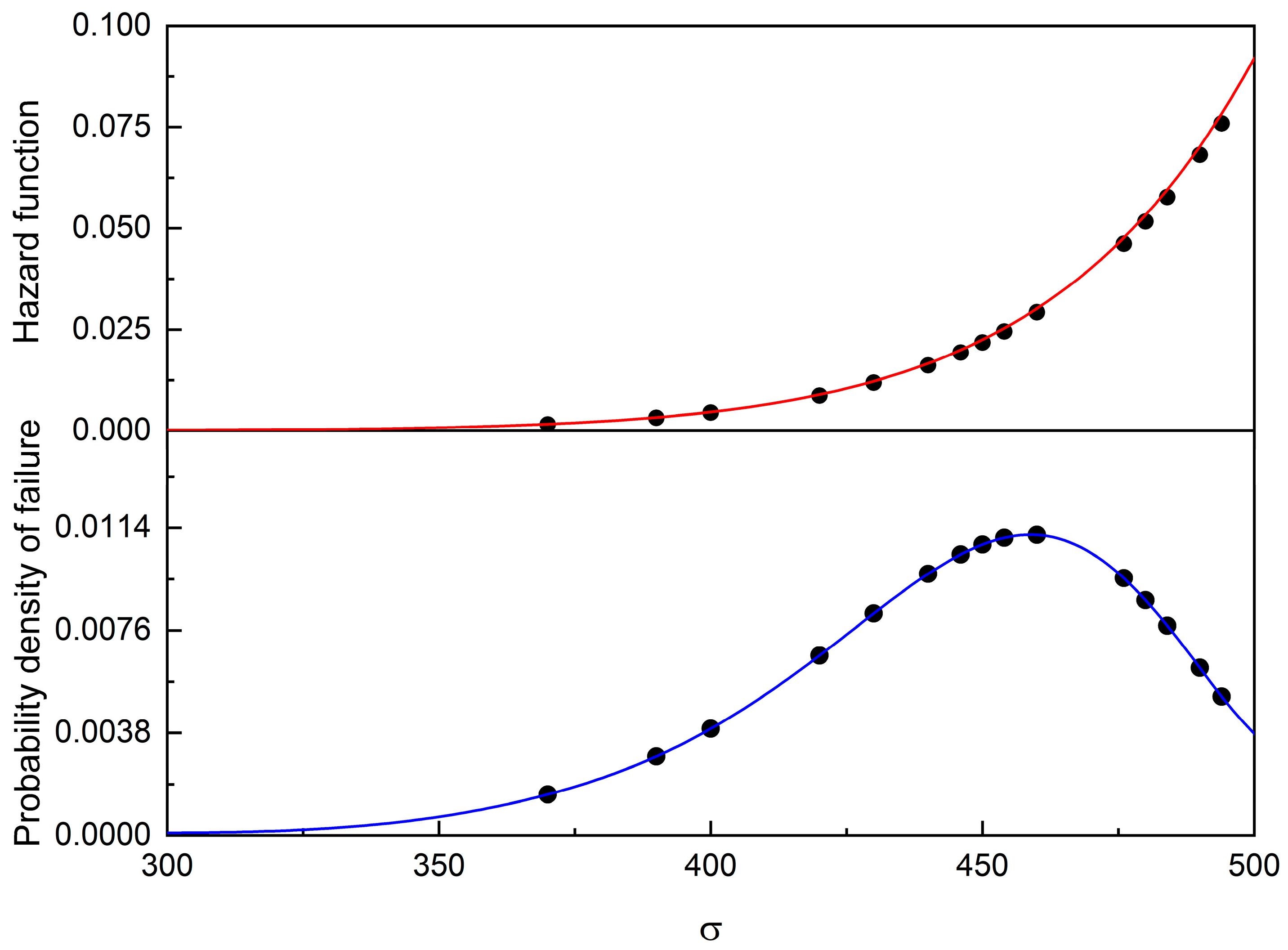
The hazard function, which describes the “conditional density”, i.e., the conditional distribution of a random variable, given that the event has not yet occurred, and the failure distribution, i.e., the probability density of failures, are shown in Figure 10.

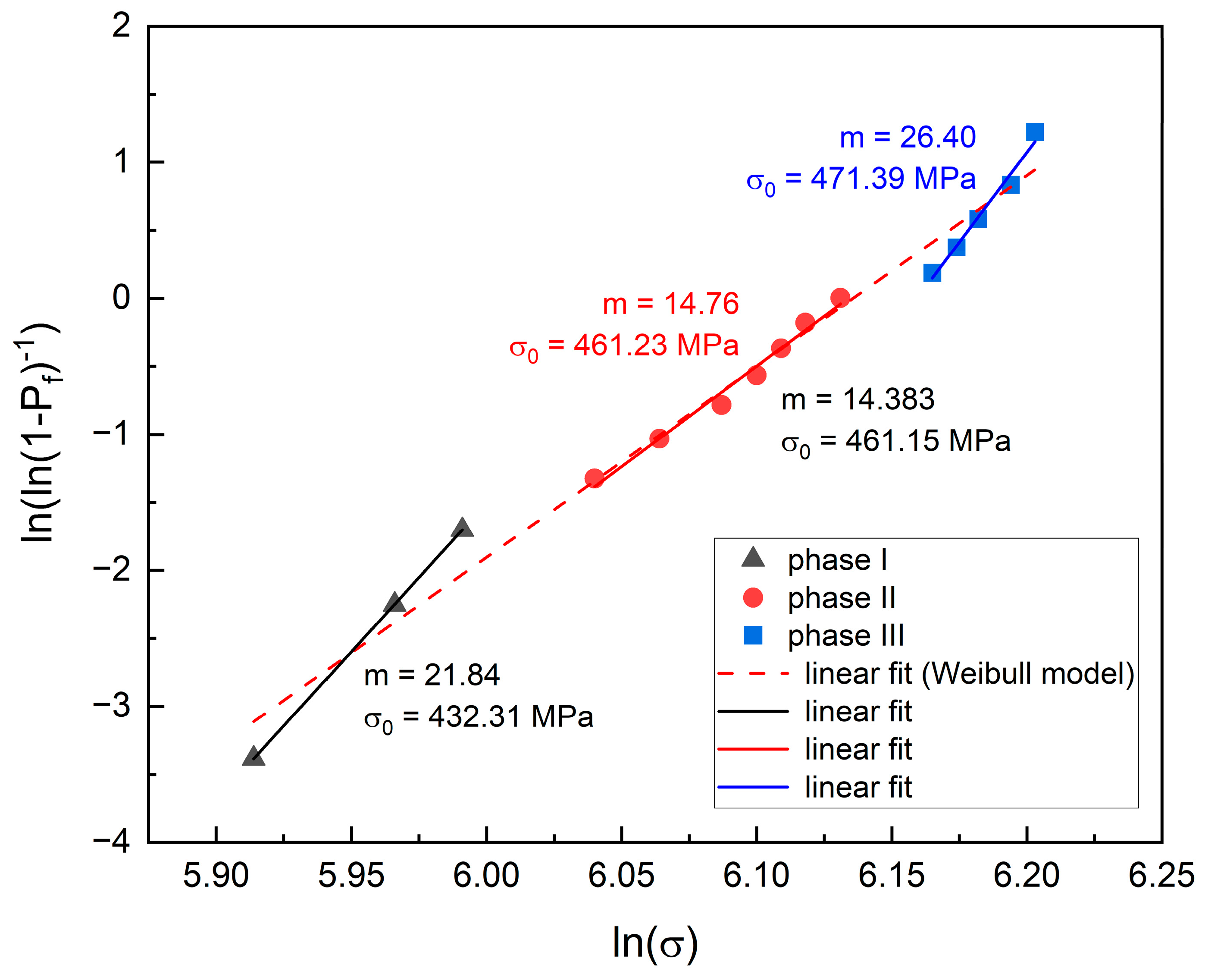
An examination of the graphs shown in Figure 8 and Figure 9 suggests that despite the high-quality fit, the scattering of the points from the Weibull model reveals a characteristic feature—splitting data into three groups. Well-defined groups of the points suggest that the Weibull model consists of three components as shown in Figure 11 and listed in

Table 5. The results of the linear fitting of three phases, along with the Weibull distribution parameters.

Phase	Phase Content, %	Fit Parameters		Statistics of the Fit			Weibull Distribution Parameters		Δm *, deg	Median, GPa
		a0	a1	r	s	Reduced χ2	m	σ₀, MPa
I	3.1%	21.838 ± 0.027	−132.538 ± 0.162	1.000	0.0015	2.302 × 10−6	21.84 ± 0.03	432.31 ± 0.19	1.356	425.12
II	92.5%	14.757 ± 0.845	−90.518 ± 5.149	0.992	0.0657	0.0043	14.76 ± 0.85	461.21 ± 7.49	0.100	449.90
III	4.4%	26.402 ± 2.195	−162.617 ± 13.573	0.989	0.0667	0.0045	26.40 ± 2.20	471.39 ± 15.58	1.808	464.89

* The difference between the slope of the total Weibull model and linear fit (phase I, II, or III) converted to degrees.

.

The slope of all three lines shown in Figure 11 is positive, but only the slope of the points in the middle part, shown in solid red, resembles those of the whole Weibull distribution (dashed line). The three lower points delineate phase I, the subsequent seven points delineate phase II, and the final five points delineate phase III. The Weibull modulus is different for each phase, Table 5. In the lower range, m is nearly 21.84, in the middle, it does not exceed 14.76, and in the upper range, it reaches 26.4. Although the differences in the m values may seem large, a comparison of the differences between the slope of the total Weibull model and each linear fit (phase I, II, or III) converted to degrees (inclination angles in degrees), Δm, shows that they are small. The percentages of phases are listed in the table. The characteristic strength values estimated based on these data are 432.31, 461.21, and 471.39 MPa, respectively. Thus, the three lower points (370, 390, and 400) reveal a greater influence of the m-phase, seven points in the middle of the graph reveal a mixture of the m-phase and t-phase, and the upper five (476, 480, 484, 490, and 494) reveal the larger influence of the t-phase. In each of them, the Weibull modulus is slightly different, the highest for the upper and the smallest for the middle part. The variation in the Weibull distribution parameters seems to be related to the temperature gradient during sintering, which in turn is related to the grain size.

3.4. Hardness Analysis

The procedure previously described was employed once more in order to analyze the distribution of the values of hardness. The results of the Vickers hardness measurement are collected in

Table 6. Vickers hardness results and parameters of the Weibull distribution for the sintered samples of ZrO₂–5 wt.% CeO₂.

Experiment No.	HV10, GPa	ln(ln(1 − Pf)−1)
1	17.5 ± 0.5	−3.218
2	18.2 ± 0.5	−2.355
3	18.65 ± 0.5	−2.068
4	19.2 ± 0.5	−1.349
5	19.32 ± 0.5	–1.061
6	20.2 ± 0.5	–0.630
7	20.35 ± 0.5	–0.486
8	20.65 ± 0.5	–0.342
9	21.55 ± 0.5	–0.198
10	21.8 ± 0.5	–0.054
11	22.2 ± 0.5	0.377
12	22.5 ± 0.5	0.521
13	22.55 ± 0.5	0.665
14	23.2 ± 0.5	0.809
15	23.25 ± 0.5	0.953

.

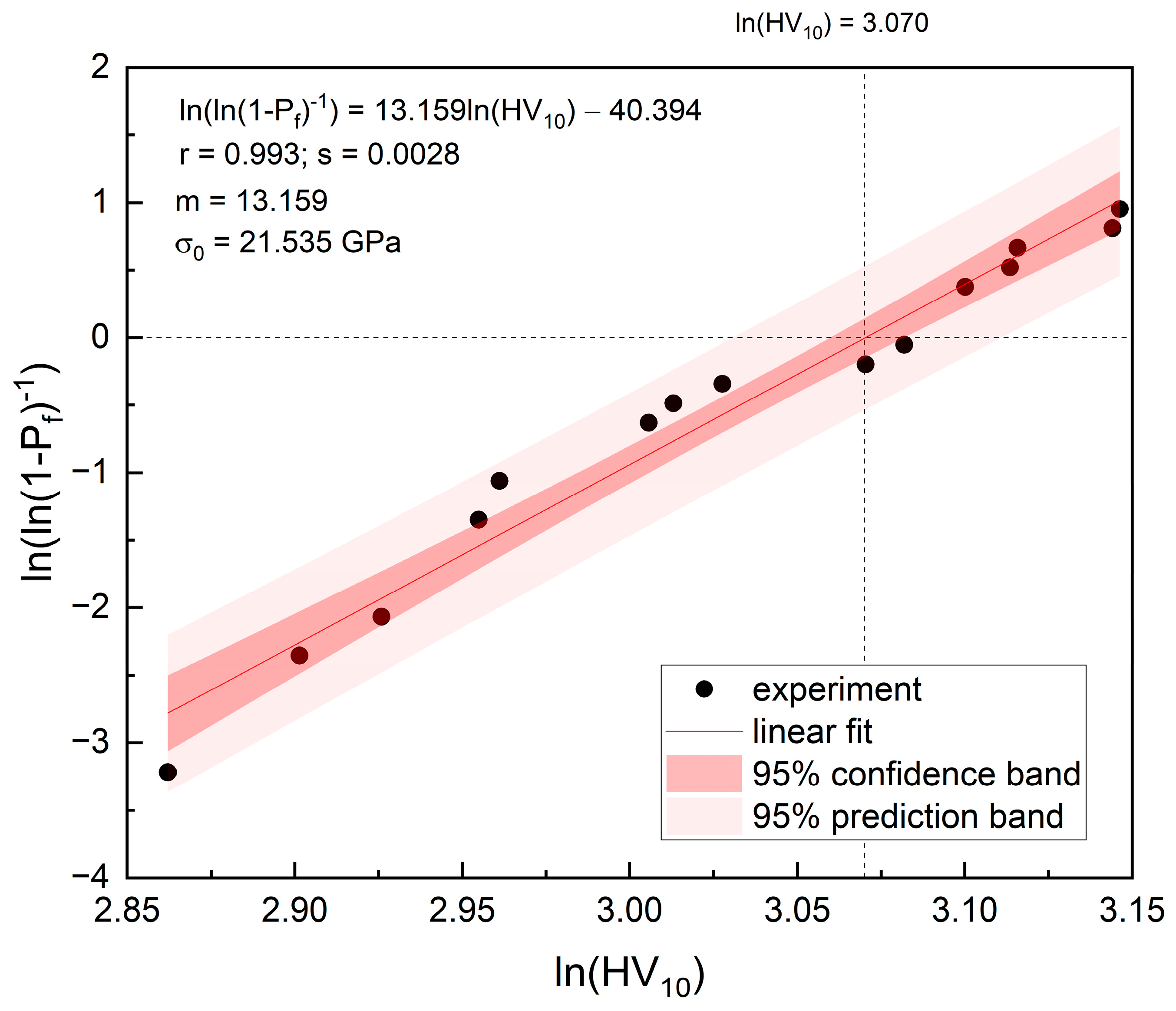
Figure 12 shows a Weibull graph, where y = ln(ln(1 − P_f)⁻¹) represents the double logarithmic transformation of the cumulative probability of failure and x = ln(HV₁₀) describes the natural logarithm of the failure of Vicker hardness. The black dots correspond to the experimental data points. The linear regression model, fitted to the data points, yielded the parameters describing the Weibull distribution listed in

Table 7. The parameters of the Weibull distribution of the hardness for ZrO₂–5 wt.% CeO₂ sintered sample.

Fit Parameters		Statistics of the Fit			Weibull Distribution Parameters
a0	a1	r	s	Reduced χ2	m	HV10, GPa
13.159 ± 3.43 × 10−6	−40.394 ± 2.092	0.999	0.0052	1.14 × 10−14	13.159 ± 3.43 × 10−6	21.535 ± 4.21 × 10−6

.

The relatively high Weibull modulus, m, of 13.159 suggests a narrow range of the hardness values, indicating a constant material hardness. The scale parameter σ₀, that does not exceed 21.535 GPa, is the characteristic hardness value reached or exceeded by as much as 63.2% of the population. The value of the Weibull modulus of 13.159 GPa is consistent with results obtained from the bending strength analysis presented in Section 3.3 and with those published in other reports [44,45,46].

The expected value to failure (mean value to failure) was calculated based on Equation (8). The average durability of the sample in terms of hardness measured by the expected value to failure is equal to 20.079 GPa,

Table 8. The statistical parameters of the Weibull distribution of the hardness for ZrO₂–5 wt.% CeO₂ sintered sample.

Mean, GPa	Median, GPa	Mode, GPa	Standard Deviation, GPa
20.079	20.943	21.456	1.919

.

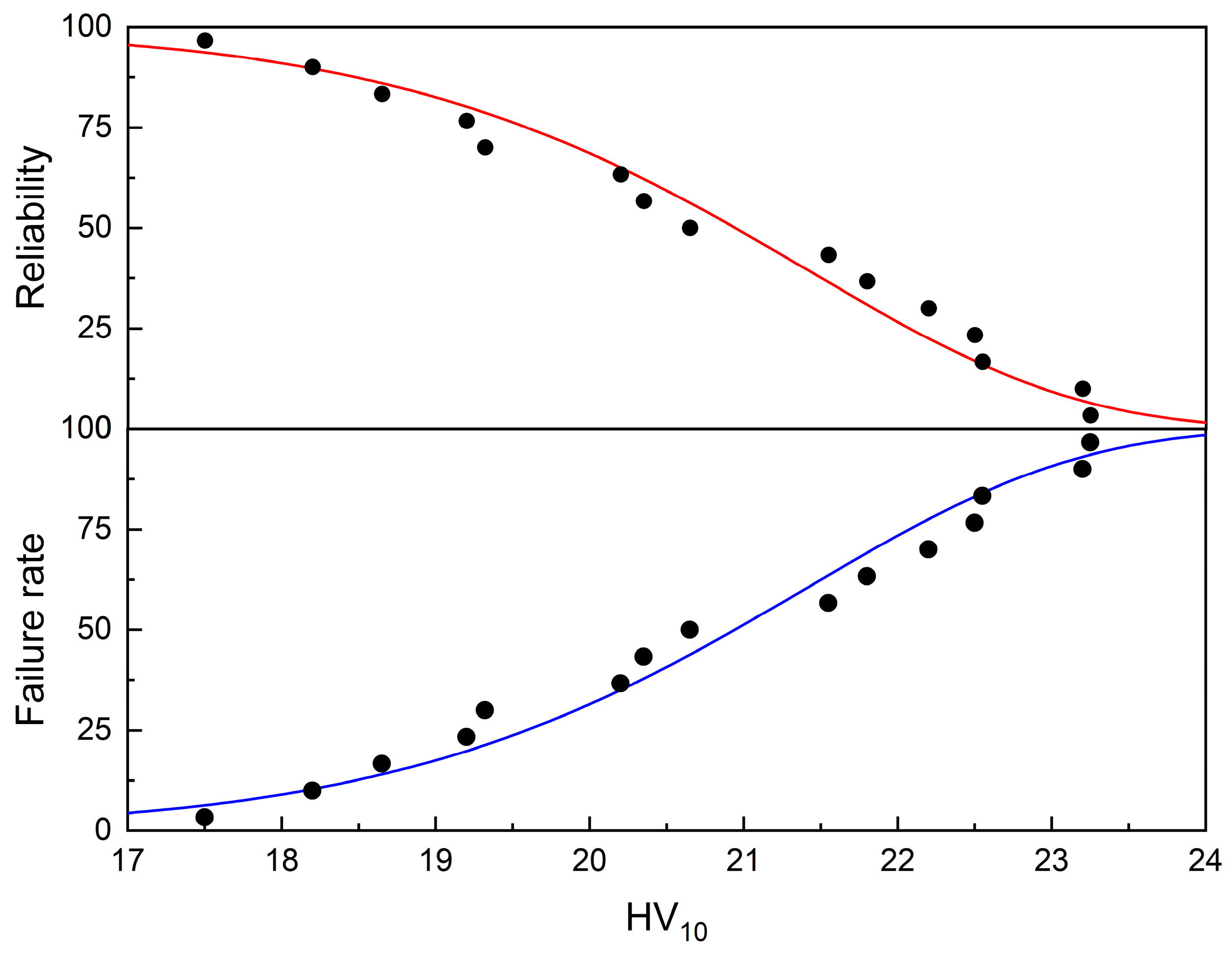
The median and the mean are almost identical, suggesting a moderately symmetrical distribution. The reliability function (the probability that the sample will keep its properties without failure) as well as failure function (the probability of failure) are shown in Figure 13. (Both were plotted based on the parameters from the linear fit shown in Figure 12).

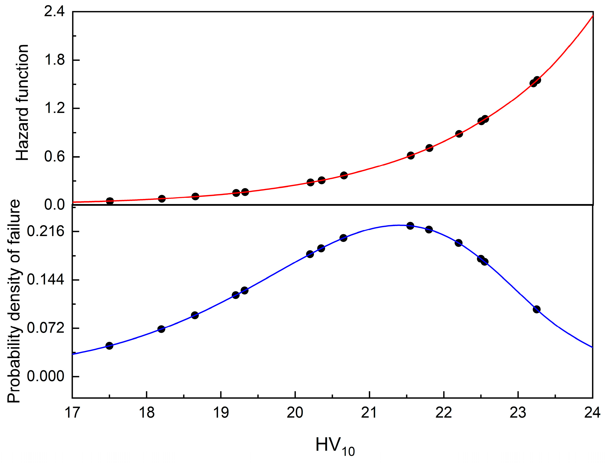
The failure function, widely known as the hazard rate, and the probability density of failure are shown in Figure 14.

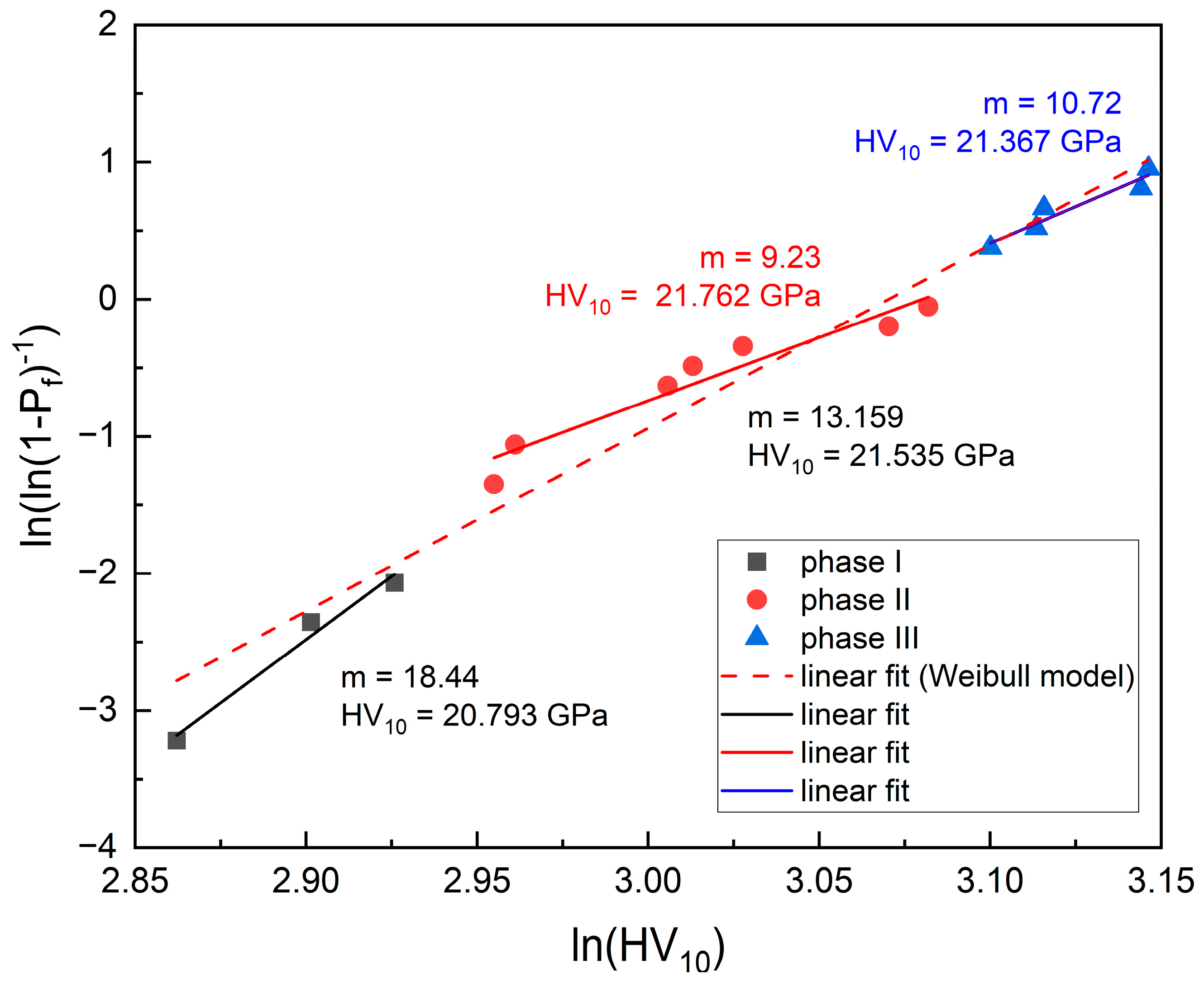
A thorough analysis of the data from the Weibull model depicted in Figure 12 reveals the presence of three distinct groups in the distribution. This indicates the Weibull model comprises three components, as illustrated in Figure 15 and listed in

Table 9. The results of the linear fitting of three regions, along with the derived Weibull distribution parameters.

Phase	Phase Content, %	Fitting Parameters		Statistics of the Fit			Weibull Distribution Parameters		Δm * [deg]	Median
		a0	a1	r	s	Reduced χ2	m	HV10, GPa
I	0.5%	18.438 ± 2.75	−55.952 ± 7.967	0.9782	0.125	0.0156	18.438 ± 2.75	20.793 ± 3.38	1.24	20.384
II	99.1%	9.225 ± 1.161	−28.415 ± 3.502	0.9626	0.138	0.0193	9.225 ± 1.161	21.762 ± 4.19	−1.84	21.648
III	0.4%	10.718 ± 1.875	−32.817 ± 5.856	0.9159	0.076	0.0058	10.718 ± 1.875	21.367 ± 6.77	−0.98	20.648

* The difference between the slope of the total Weibull model and linear fit (phase I, II, or III) converted to degrees.

.

Figure 15 shows that all three lines have a positive slope, but only the blue points at the top match the whole dataset slope (dashed line). Thus, the Weibull model describes in fact three different distributions. The three lower points delineate phase I, the subsequent seven points delineate phase II, and the final five points delineate phase III. The Weibull modulus is different in each phase, Table 9. In the lower range, m is almost 18.44, in the middle, it does not exceed 9.23, and in the upper range, it reaches 10.72. Although the differences in the m values may seem large, a comparison of the differences between the slope of the total Weibull model and each linear fit (phase I, II, or III) converted to degrees (inclination angles in degrees), Δm, shows that they are small. The percentages of the phases are listed in the table. The characteristic hardnesses estimated based on these data are equal to 20.703, 21.762, and 21.367 GPa, respectively. Thus, the three lower points (370, 390, and 400; depicted in black) reveal a negligible influence of the m-phase, which has lower symmetry. The seven points in the middle of the graph (depicted in red) reveal a mixture of the m-phase and t-phase, and the top five (476, 480, 484, 490, and 494; depicted in blue) reveal a negligible influence of the t-phase. The difference between the hardness in the phases I, II, and III is negligible. Thus, the hardness is very stable.

The Weibull modulus, when greater than 4, is indicative of the inherent property limitations of materials, e.g., ceramic brittleness. However, it also is indicative of severe problems in the manufacturing process, or of minor variability in the manufacturing process or in the material itself. The results obtained indicate a high homogeneity of the material tested, not only as regards strength but also hardness. Thus, the high values of the Weibull modulus suggest that the nanopowder studied is high quality and reliable in terms of hardness and strength.

4. Conclusions

From the performed experiments and statistical analysis of the results, the following conclusions can be derived. The high value of shape parameter m = 14.383 indicated that the bending strength of ZrO₂ stabilized with 5 wt.% CeO₂ samples exhibited low variability. This result suggested consistent material performance. The characteristic strength σ₀ = 461.15 MPa was relatively high, which proved that the material could withstand substantial stress before failure.

The linearity of the plot shows a good fit to the Weibull distribution, suggesting that the model was appropriate for prediction of the probability of failure under respective loads. The small scattering of the experimental points from the straight line indicates the high quality and repeatability of the manufacturing process, and subsequent uniformity of the material properties.

The high value of the shape parameter indicates the uniformity and repeatability of the hardness reached by the fabricated specimens. A scale parameter of σ₀ = 21.535 GPa suggests the material can maintain high hardness levels under typical work conditions. Based on the hardness and strength Weibull distribution analysis, it can be concluded that the proper quality of ZrO₂–5 wt.% CeO₂ was reached and can be kept in the subsequent stages of the research program on the electroconsolidation process. In particular, the analysis provided a solid ground for preparation of the modified, improved device prototype.

It appears that the variability of the Weibull distribution parameters is associated with the temperature gradient during the process of sintering. The experimental evidence and statistical analysis reveal an influence of the m-phase, which has lower symmetry and, therefore, its addition make ceramic weaker and softer. Furthermore, their progressive replacement by the t-phase, which has higher symmetry, makes ceramic both harder and stronger. Reducing the mol% increases the risk of the appearance of the highest addition of the monoclinic phase; increasing it is unfavorable from the point of view of the sintering process. Statistical and manufacturing evidence suggests that the choice of 5%/mol is optimal.

The results of the research demonstrated that the sintered specimens sintered with a novel electroconsolidation method out of ceria-stabilized zirconia powder exhibited high strength and retained high hardness. Repeatable sintering conditions and the addition of 5 mol% CeO₂ ensured the reproducibility of the high-quality properties of the tested ceramic. They reveal the high sensitivity of the nanopowders (their structure and grain size) to the temperature gradient.

Further improvement can be reached through optimization of the synthesis route, modification of the ceria content, and experiments with altered sintering conditions. In particular, it could be expected that improved structural homogeneity and nanoscale features might be reached through optimal heating rate control, related to the respective phases of the sintering process. Works on further improvement of the electroconsolidation process and respective zirconia-based ceramics’ properties and reproducibility are planned.